Article

Modeling Exhaust Emissions in Older Vehicles in the Era of New Technologies

by
Maksymilian Mądziel
Faculty of Mechanical Engineering and Aeronautics, Rzeszow University of Technology, 35-959 Rzeszow, Poland
Energies 2024, 17(19), 4924; https://doi.org/10.3390/en17194924
Submission received: 6 September 2024 / Revised: 24 September 2024 / Accepted: 30 September 2024 / Published: 1 October 2024
(This article belongs to the Section B: Energy and Environment)

Abstract

:
In response to increasing environmental demands, modeling emissions from older vehicles presents a significant challenge. This paper introduces an innovative methodology that takes advantage of advanced AI and machine learning techniques to develop precise emission models for older vehicles. This study analyzed data from road tests and the OBDII diagnostic interface, focusing on CO2, CO, THC, and NOx emissions under both cold and warm engine conditions. The key results showed that random forest regression provided the best predictions for THC in a cold engine (R2: 0.76), while polynomial regression excelled for CO2 (R2: 0.93). For warm engines, polynomial regression performed best for CO2 (R2: 0.95), and gradient boosting delivered results for THC (R2: 0.66). Although prediction accuracy varied by emission compound and engine state, the models consistently demonstrated high precision, offering a robust tool for managing emissions from aging vehicle fleets. These models offer valuable information for transportation policy and pollution reduction strategies, particularly in urban areas.

1. Introduction

In the era of rapid advancement in automotive technology, the focus has changed to achieving excellence in performance, safety, and balanced environmental development. Modern vehicles are now equipped with advanced emission control systems that significantly reduce pollutants [1,2]. However, older vehicles, which were manufactured before these innovations were introduced, still constitute a substantial part of the global vehicle fleet and continue to pose a challenge in emission management [3].
Road transportation remains a major contributor to global air pollution, particularly due to emissions from internal combustion engines [4,5]. Exhaust gases from vehicles release harmful pollutants such as carbon dioxide (CO2), nitrogen oxides (NOx), carbon monoxide (CO), and particulate matter (PM), all of which have detrimental effects on human health and the environment [6,7]. For example, NOx emissions contribute to the formation of ground-level ozone and smog, while particulate matter has been linked to respiratory diseases and premature mortality [8,9]. Older vehicles, which were manufactured prior to the implementation of stringent emission standards, are especially problematic as they tend to emit these pollutants in much higher quantities compared to newer models equipped with advanced emission control technologies [10,11]. As highlighted in the study [12], the impact of vehicle emissions on air quality is a pressing concern, and the aging global fleet of vehicles exacerbates this issue by contributing disproportionately to pollution levels.
Older vehicles lacking modern emission control technologies typically emit higher levels of pollutants, which complicates the precise modeling and regulation of their exhaust emissions [13,14]. Vehicles without advanced technologies such as catalytic converters or exhaust gas recirculation systems produce significantly higher levels of pollutants compared to contemporary models [15,16]. Historically, when emission standards were less stringent, engine designs and combustion systems were not optimized to minimize harmful emissions such as carbon dioxide (CO2), nitrogen oxides (NOx), carbon monoxide (CO), or hydrocarbons (THC) [17]. As a result, these vehicles generate higher amounts of these pollutants, presenting a significant challenge in modeling their emissions in the context of modern environmental standards [18]. Furthermore, precise regulation of vehicle emissions is problematic because the absence of advanced control technologies means that pollutants emitted are less uniform and can vary significantly depending on the technical condition of the vehicle, the operating conditions, and the type of fuel [19,20]. This makes it more difficult to establish accurate emission profiles and forecast their environmental impact. Additionally, older vehicles can exhibit significant variability in emissions over time [21], further complicating the application of standard modeling methods and the evaluation of remedial measures [22,23].
From a modeling perspective, there is also a challenge associated with the lack of high-quality data for these vehicles, which could be used for the precise calibration of emission models. Consequently, standard emission models developed for modern vehicles may be inappropriate or inadequate for older vehicles, leading to inaccurate forecasts and inefficient emission management [24]. This requires the development of specific modeling methods that take into account the historical technical conditions and emission characteristics of older vehicles to effectively monitor and control their environmental impact. Artificial intelligence (AI) thus represents an opportunity to develop new emission models for older vehicles, allowing for more accurate predictions of harmful exhaust components.
Artificial intelligence (AI) and machine learning (ML) techniques have a significant impact on the emission modeling process, particularly with respect to older vehicles [25]. Traditional emission modeling methods often relied on precise but limited chemical and physical equations. On the contrary, AI and ML enable a more dynamic and adaptive approach [26,27]. Machine learning algorithms can analyze large amounts of data from various sources, such as road tests, vehicle sensors, and historical data, allowing more accurate prediction of emissions in a wide range of operational conditions [28]. For older vehicles that may lack modern emission monitoring systems, ML can help create predictive models based on data collected from tests and simulations, even if these vehicles are not equipped with advanced sensors [29,30]. Algorithms such as neural networks and random forests can capture complex patterns and relationships that would be difficult to determine using traditional methods [31,32]. Therefore, AI and ML not only improve the accuracy of emission forecasts but also facilitate the development of more effective emission reduction strategies for older vehicles that may not meet today’s environmental standards.
There is a body of work that addresses emission modeling issues for older vehicles; however, it focuses primarily on emissions related to the types of fuels used. For example, a study [33] develops advanced models for predicting CO2 emissions for vehicles powered by compressed natural gas (CNG) in response to stringent global environmental regulations. Using XGBoost within the Optuna Python framework and data from chassis dynamometer and road tests, the study achieves high model precision, providing critical insights for environmental decision-makers and urban transportation planning.
The application of artificial intelligence techniques to modeling emissions for older vehicles powered by LPG is presented in another work [34]. This study introduces a new methodology to create CO2 emission models for vehicles powered by LPG based on road test data and the OBDII diagnostic interface. Using machine learning methods, the model shows good precision, which proves useful for CO2 emission analysis and the creation of emission maps for urban areas, achieving R2 coefficients of 0.61 and an MSE of 0.77. The need to develop new emission models in the context of an aging vehicle fleet is also highlighted in the work referred to as [35]. This study investigates the impact of aging processes on vehicle emissions, focusing on the changes in aerosol pollutants resulting from these processes. The authors describe initial emission properties such as hygroscopicity, particle size distribution, and chemical composition, as well as changes in these properties as a result of physical actions and photochemical reactions. The study also discusses the impact of vehicle driving cycles and emission control technologies and fuels and identifies areas for future research that could support the control of air pollution related to vehicle emissions. The increase in emissions due to the increase in mileage of older vehicles is further illustrated in the study cited as [36]. Another paper on PEMS emissions modeling for older vehicles is [37]. This study focuses on modeling emissions for older Euro 5 vehicles, highlighting the importance of accurate transport emission factors in addressing air pollution and climate change. The research uses map-based simulations to develop emission factors for CO2, NOx, and CO using real-world emissions data obtained from a portable emission measurement system (PEMS). A dynamic simulation model of vehicles calculates these emission factors, integrating data from various parameters such as fuel type, emissions regulations, and aftertreatment systems. The work, which touches on the fact that current models in use do not always reproduce emissions well for an older fleet of vehicles, is [38]. This paper presents a significant advancement in mobile source emissions modeling through the modification of the US-EPA MOVES model for application in Hyderabad, India. Recognizing that the default “Federal Test Procedure-Based Driving Cycle” does not accurately reflect local driving conditions, the study introduces a “Modified Indian Driving Cycle” along with local light-duty vehicle-specific cycles to update emission rates. The findings indicate that, on average, emission rates in India are substantially higher than the default US rates, with CO, HC, and NOx emissions being 9.54, 8.37, and 9.45 times higher, respectively.
A review of existing research reveals significant gaps in the literature. Many current studies focus on modeling individual exhaust components, while this study addresses groups of components. In addition, numerous works focus on modeling specific vehicle fuel technologies without considering the impact of vehicle age. Furthermore, none of the existing studies have explored the issue of clustering of input data in the context of emission modeling.
In light of these gaps, this study focuses on the challenge of modeling emissions from older vehicles from a reverse engineering perspective. The emission modeling process employs modern methods, including artificial intelligence techniques using the Python programming language. For the first time, the input data have been clustered, enhancing the predictive capabilities of the models. Emissions have been classified into two main groups: for cold and warm engine conditions. This detailed approach allows precise replication of older vehicle emissions and can be scaled to larger vehicle groups or emission databases, facilitating the creation of more accurate predictive models. These models have been validated, and their potential applications have been discussed, including their use in shaping transportation policy, particularly with respect to the fleet of aging vehicles.

2. Methods

The general outline of the work is presented in Figure 1. This study initially involved selecting a vehicle that could represent the older fleet of vehicles that did not meet the new stringent emission standards. The next step was to choose a test route and conduct road tests. These tests were performed using the portable emission measurement system (PEMS), which collected emission data, vehicle location, and environmental data at a frequency of 1 Hz. The data were then saved in.csv format for further processing using the Python programming language. All analyses and data processing were performed in the Google Colab programming environment. A key aspect of this process was the clustering of input data for emission modeling. This approach facilitates the creation of better and more accurate emission models. Subsequently, emission models were developed using machine learning techniques based on the appropriate clusters of input data. The final stage of the work demonstrates the potential applications of the developed models.

2.1. Research Vehicle, Route, and Apparatus Used

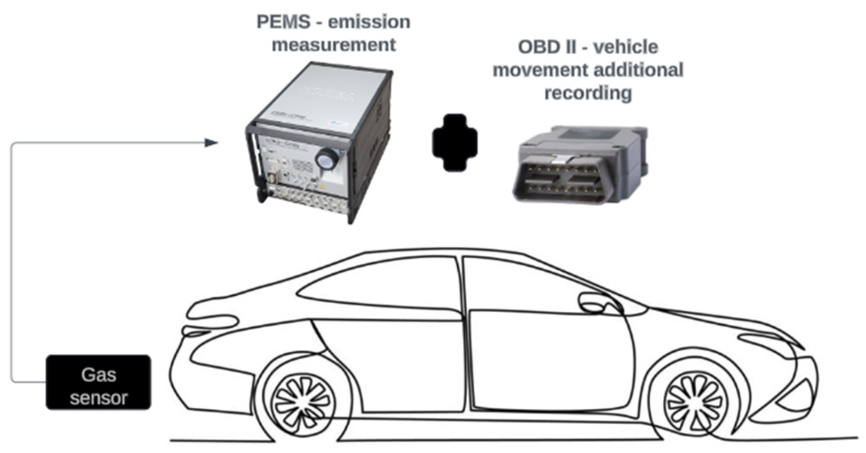
The primary objective of this work was to develop a new methodology for creating emission models for vehicles, specifically tailored for older models. The vehicle studied is a Euro 2 class passenger car, manufactured in 1998. It is equipped with a 1598 cm3 engine that operates on spark ignition and is fueled by gasoline. The engine produces a maximum power of 88 kW at 6300 rpm and a maximum torque of 144 nm at 4500 rpm. The car features a five-speed manual transmission. The fuel supply system is a multi-point fuel injection (MPI) system, and the emission control system is a three-way catalytic converter (TWC). The vehicle weighs 1230 kg. The vehicle scheme and equipment studied are shown in Figure 2.
Emission data were collected using a portable emission measurement system (PEMS). PEMS employs various technologies to monitor exhaust emissions, including flame ionization detectors (FIDs) for hydrocarbons, NDIR spectrometers for CO and CO2, and chemiluminescence detectors (CLDs) for NO and NO2. According to EU Regulation 2017/1151, deviations between PEMS results and stationary analyzers should not exceed 15% for HC, CO, and NOx and 10% for CO2 [39,40]. The PEMS unit is installed in the vehicle’s trunk, with sensors connected to the exhaust pipe, and the sample extraction line must be heated to 190 °C [41,42]. In addition, the system monitors air temperature and humidity and utilizes a GPS transmitter. An OBDII interface can also be connected to the ECU for more comprehensive emission analysis.
To collect data on harmful exhaust components, a specific test route was selected for the initial phase of the work, where emission levels were recorded. The data obtained from the actual drives were subsequently used to develop emission models for the selected substances. Given the need for a large amount of input data, the test route was 40 km long, allowing the collection of sufficient information for precise modeling. The route included driving through the city of Rzeszów, the S19 expressway around Rzeszów, and a section of the A4 motorway. This varied route provided a wide range of data, reflecting different engine operating conditions and variable speeds. As a result, accurate information on harmful exhaust emissions was obtained under various driving and operational conditions.

2.2. Software Used and Data Processing

Data analysis and model execution were performed in the Google Collaboration environment. Google Colaboratory, also known as Google Colab, is a free service from Google that enables the creation and execution of interactive Jupyter notebooks in the cloud [43]. This platform provides an integrated environment that supports Python coding and documentation of results in notebooks, facilitating collaboration and project sharing. With free access to GPU and TPU units, Google Colab significantly accelerates computations related to training machine learning models [44].
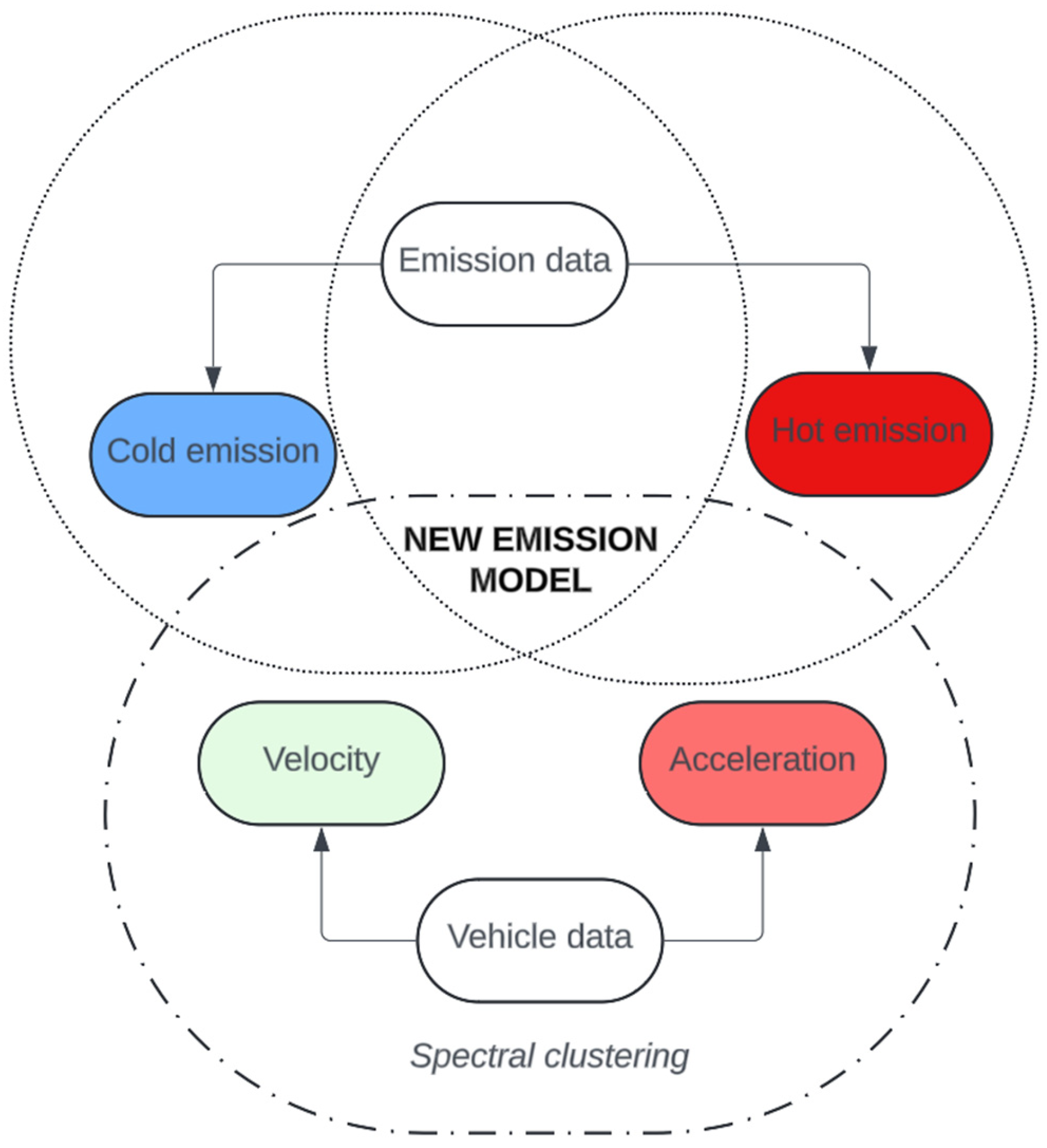
A key aspect of the innovative modeling approach presented was the selection of explanatory variables to develop CO2, CO, THC, and NOx emission models. To create the most universal models, it was decided that the explanatory variables for emissions would be fundamental vehicle parameters, namely speed and acceleration. The overall process for handling emission and vehicle movement data in the context of modeling is illustrated in Figure 3.
Figure 3 presents an overview of the data processing steps used to create emission models for selected exhaust components. For the vehicle’s dynamic variables, which will serve as explanatory variables in the model, velocity and acceleration were chosen. These data will undergo spectral clustering to identify subsets for which more accurate emission models for older vehicles can be developed. Additionally, the data will be divided into cold and hot emission datasets due to the different characteristics observed in their generation.
In this context, clustering of the data was used for the first time to create the most accurate emission models possible. Vehicles operating at different speeds and acceleration dynamics generate varying levels of emissions, especially older vehicles, which may also encounter problems such as fuel system problems and higher fuel doses. Spectral clustering was used for data clustering purposes. The emissions data were further divided into categories for the cold and warmed engine states.
The use of data clustering techniques, such as spectral clustering, in emission modeling offers several benefits, particularly in the analysis of emissions from warm engines. Clustering allows for the identification of natural groups within the data that may correspond to different engine operating conditions and emission levels [45]. For a warm engine, different clusters may reflect various speeds and acceleration ranges, each having a different impact on the levels of harmful emissions. The application of spectral clustering in this context has several notable advantages. First, spectral clustering is capable of capturing complex, nonlinear structures in the data [46,47], which is particularly useful for emissions modeling, where relationships between variables can be intricate. Second, clustering facilitates a better understanding of how different engine operating conditions affect emission levels, potentially leading to more accurate predictive models and more effective emission control strategies.

3. Results

3.1. Exhaust Emission Results from Road Tests

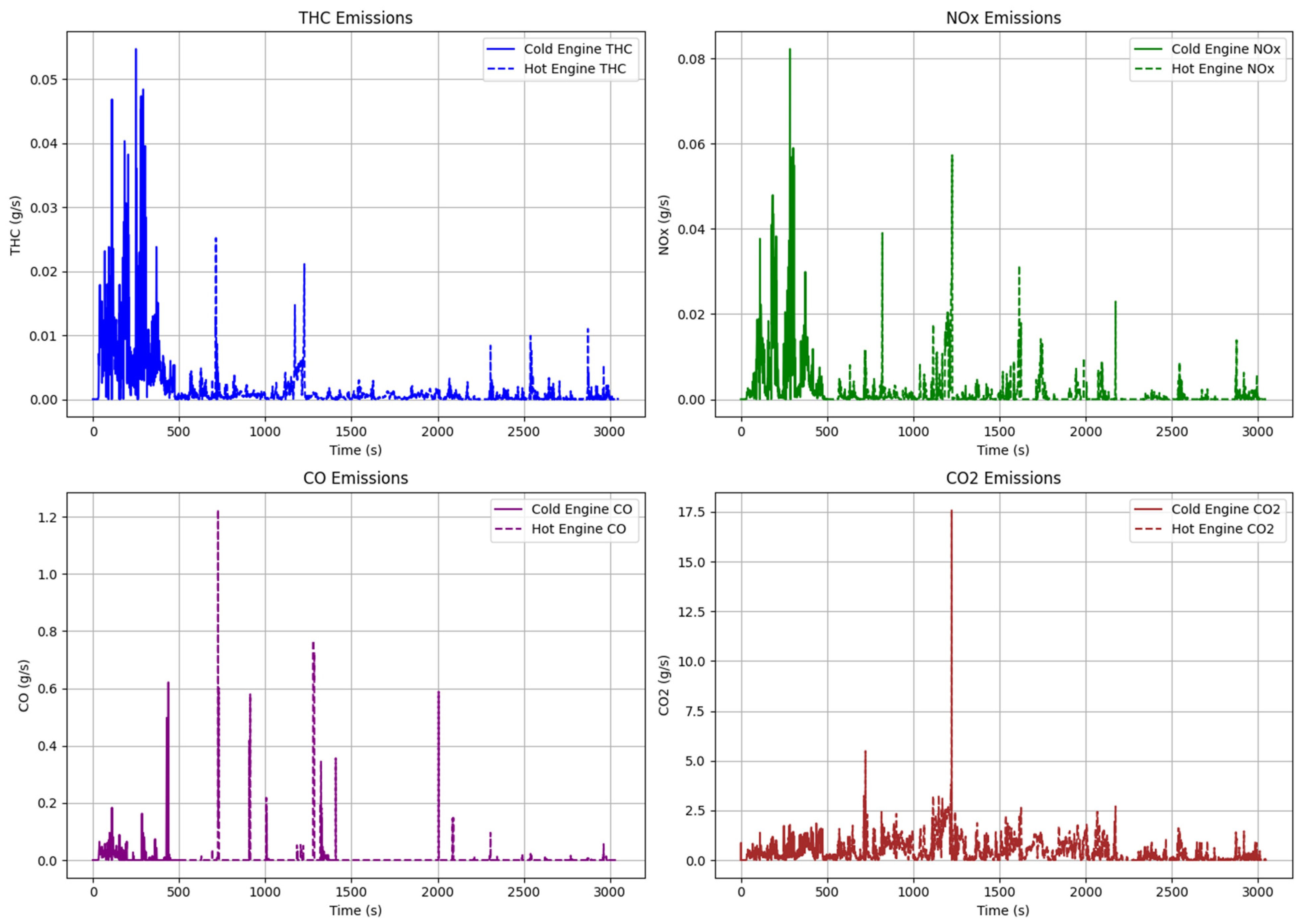
Figure 4 presents the THC, NOx, CO, and CO2 emission levels recorded during the tests. Notably, for THC and NOx, significantly higher emission values are observed for the cold engine, making the distinction between cold and hot emission data crucial for accurate modeling. CO emissions for the cold engine also contribute more to total emissions, whereas CO2 emissions remain at the same level as for the heated engine. The increase in THC, NOx, and CO emissions from the cold engine is closely related to the unheated exhaust emission control system of the vehicle. When the engine has not yet reached its optimal operating temperature, the combustion process is less efficient, leading to higher levels of hydrocarbons (THC) and nitrogen oxides (NOx) in the exhaust. An unheated catalyst and other components of the emission control system are not yet operating at full efficiency, increasing the emission of harmful substances [48,49]. For carbon monoxide (CO) emissions, the higher values for the cold engine also indicate inefficient combustion, typical of a cold engine, where the fuel–air mixture is not optimally burned. On the other hand, CO2 emissions, which are primarily correlated with total fuel consumption, show less pronounced differences between cold and heated engines. Although fuel consumption is slightly higher for the cold engine, as it requires more fuel to reach the optimal operating temperature, differences in CO2 emissions are less noticeable. CO2 is a direct indicator of the total amount of fuel burned, and these differences are less pronounced compared to other pollutants, which are more sensitive to the technical condition of the engine and the operating temperature. In cold engine conditions, despite lower combustion temperatures that generally reduce NOx formation, higher NOx emissions were observed (as shown in Figure 4). This can be attributed to the delayed activation of the vehicle’s emission control systems, such as the catalytic converter, which operates less efficiently when cold. Although NOx formation in the combustion chamber is lower due to reduced temperatures, the unheated catalyst is unable to effectively convert NOx into less harmful gases, resulting in elevated NOx emissions [50]. Additionally, during cold starts, the engine operates under transient conditions with a richer air–fuel mixture, which further contributes to the emission of NOx and other pollutants until optimal operating temperatures are reached.
Therefore, analysis of CO2 emissions may not fully reflect the impact of engine state on exhaust emissions, whereas THC, NOx, and CO are more sensitive to changes in combustion efficiency and the operation of emission control systems.
The dataset of emission inputs presented in Figure 4 was used to train the model. These data were divided into “cold” and “hot” emissions. Additionally, the data were further divided based on the clusters created for the explanatory variables, namely speed (V) and acceleration (a).

3.2. Clustering of Model Learning Inputs

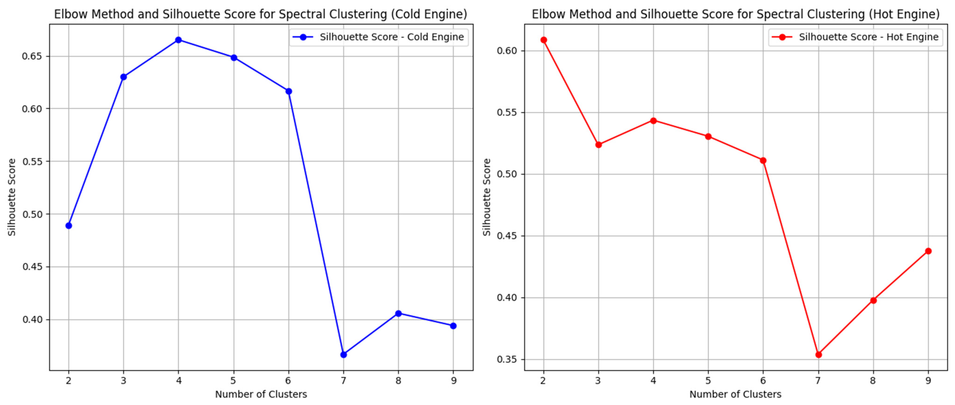
To analyze emissions for different engine operating conditions, the spectral clustering algorithm was employed. This method allows for the identification of the optimal number of clusters in the data representing emission levels, based on explanatory variables such as speed (V) and acceleration (a). The choice of this method was motivated by the need to capture complex nonlinear patterns in the data that are difficult to identify using traditional clustering methods, such as k-means [51,52]. To determine the optimal number of clusters, the elbow method and silhouette coefficient analysis were used, calculated for various numbers of clusters (ranging from two to nine), which allowed the evaluation of cluster cohesion (Figure 5).
Figure 5 illustrates the evaluation of the silhouette score for different numbers of clusters (ranging from two to nine) used in spectral clustering. The silhouette score is a measure of cluster quality, assessing how well points are grouped within a cluster and how distinct they are from points in other clusters [53,54]. The horizontal axis of the chart represents the number of clusters, while the vertical axis shows the silhouette score value. From the shape of the chart for cold emissions, it can be observed that the highest silhouette scores are achieved with four and five clusters, with the highest value of approximately 0.67 for four clusters. This suggests that four clusters provide the most effective clustering, indicating that it is the optimal number of clusters for the spectral clustering method used. The silhouette score for cold emissions decreases significantly with six clusters and remains at a lower level for larger numbers of clusters, indicating that a greater number of clusters leads to a less distinct and effective data partition. Thus, the optimal number of clusters for analysis using spectral clustering is four, as it produces the highest silhouette score, indicating the best cluster quality. However, for warm emissions, the best solution is to use two clusters.
In this study, spectral clustering was applied to analyze emissions data collected from vehicle engines. Data were initially divided into two sets according to engine temperature: cold and warm. Data for the cold engine state included the first 500 records, while the remaining records were assigned to the warm engine state.
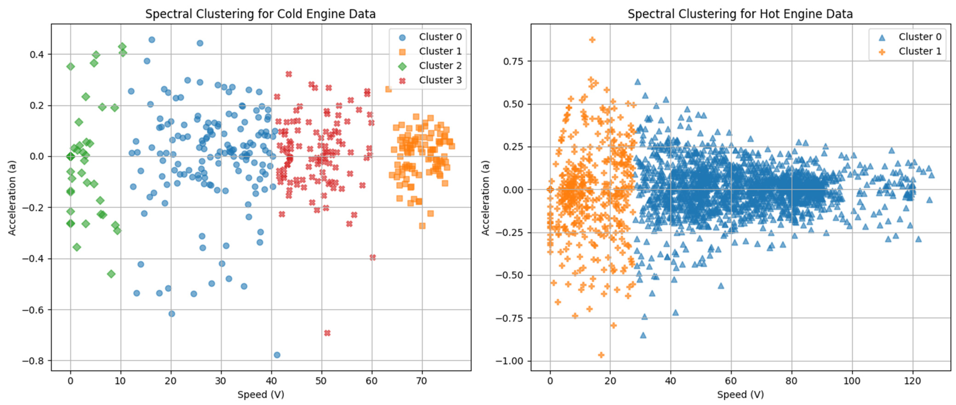
Spectral clustering was performed on each subset, with the optimal number of clusters determined on the basis of the preliminary analysis. For cold engine data, four groups were selected, while two groups were chosen for warm engine data (Figure 6). The clustering process utilized an affinity matrix based on nearest neighbors to capture the internal structure of the data.
The results shown in Figure 6 are illustrated using scatter plots, where each data point is colored according to its assignment of clusters. The data presented for the cold emission clusters were classified into four groups. These data exhibit a slightly different distribution characteristic; however, the emissions themselves are more dependent on the variables of speed and acceleration. For example, for hot CO or NOx emissions, we do not always observe a strong correlation with changes in these emissions relative to the vehicle’s dynamic parameters, as emissions may be more influenced by other factors, such as the combustion temperature of the fuel mixture, which are not considered in the model. Here, we focus on selecting universal variables that can be obtained from various sources for new trips or simulation variables. These scatter plots demonstrate how the data are grouped on the basis of the explanatory variables for future emission models, speed (V) and acceleration (a), with distinct differences between clusters clearly marked. Such visualizations provide information on clustering patterns and relationships between emission characteristics under different engine operating conditions.

3.3. Emission Modeling and Validation

For the data clusters created, emission models were developed for CO2, CO, THC, and NOx for both cold and hot engine states. The modeling process employed various regression techniques to assess its effectiveness in the context of different engine conditions. The simulation was carried out separately for data from cold and hot engines, allowing for a detailed analysis of the impact of the engine state on the prediction results.
The first step was to define the target variables and the regression models to be evaluated. The models were evaluated based on their ability to predict emissions using selected features such as vehicle speed and acceleration. Different regression methods were considered to achieve a comprehensive understanding of the relationships between variables and to accurately forecast emissions for both cold and hot engines. Linear regression, as a fundamental model, was used as a starting point to evaluate the linear relationships between vehicle features and emissions [55]. Although linear regression is simple and effective, it may not suffice for more complex, nonlinear relationships [56]. Therefore, polynomial regression was employed to model nonlinear dependencies by adding polynomial terms, potentially better capturing intricate interactions between variables. Additionally, Lasso and Ridge regressions were introduced as regularization methods to address overfitting by penalizing large model coefficients. Regularization is crucial for feature selection and improving model generalization, particularly with high-dimensional data. Decision tree regression, on the other hand, introduces a hierarchical approach to data classification that handles nonlinear relationships well, although it may be prone to overfitting if not properly pruned [57].
To further enhance prediction accuracy, random forest regression was used, which combines predictions from multiple decision trees, improving model stability and accuracy. Moreover, support vector machine (SVM) regression was included as an advanced method that utilizes kernel functions to map input features to higher dimensions, potentially capturing more complex, nonlinear relationships [58]. The testing of various regression methods allowed the comparison of their effectiveness and the selection of the most appropriate model for the prediction of emissions, considering the specificity and complexity of the data.
For regression models such as polynomial regression, the process involved creating new features through polynomial transformation and then training a linear regression model on the processed data. To ensure the robustness and reliability of the models selected for predicting the emissions, a five-fold cross-validation was performed for each model. The models and their cross-validation performance are summarized in Table 1. The results were evaluated based on the mean squared error (MSE) and the coefficient of determination (R2), providing information on the accuracy of the prediction and the fit of the model. For each target (e.g., THC, NOx, CO, and CO2) and each regression model, MSE and R2 were calculated for both cold and hot engine data. In the case of polynomial regression, the process included feature transformation, model training, and performance evaluation based on predictions and actual values. For the remaining models, the build_and_evaluate_model function was used to automatically build and assess the model, providing relevant metrics.
Mathematically, the process of creating models can be represented by the following formulas:
  • Data clustering: the dataset is partitioned into two categories: cold engine and hot engine emissions, represented mathematically as:
    D c o l d = { V i , a i ,   E c i = 1,2 , ,   D c o l d }
    D h o t = { V i , a i ,   E c i = 1,2 , ,   D h o t }
    where V is speed, a is acceleration, and Ec represents emission compound data.
  • Emission modeling: the relationship between the features (speed and acceleration) and the target emission compounds (THC, NOx, CO, and CO2) can be modeled using general regression equations:
    E c = f V , a + k
    where Ec represents the emission for compound c (THC, CO, NOx, CO2), f is a function derived from the regression model, and k denotes the error term.
The results of the best prediction methods for each emission component and engine state are presented in Table 1.
Table 1 presents the evaluation results of various regression models for predicting the emissions of four chemical compounds: THC, NOx, CO, and CO2 under both cold and hot engine conditions. For each emission compound, the model with the best performance is indicated, along with the evaluation metrics: MSE (mean squared error) and R2 (coefficient of determination). Additionally, a five-fold cross-validation was performed to ensure the robustness and generalization of the models, and the standard deviations of the cross-validation scores are reported.
For THC emissions in a cold engine, the best model was random forest regression, which achieved a mean MSE of 0.00003 ± 0.00001 and an R2 of 0.756 ± 0.014, indicating good prediction quality. For NOx, polynomial regression was the top performer with a mean MSE of 0.00005 ± 0.00002 and an R2 of 0.602 ± 0.013, reflecting a moderate model fit. For CO emissions, gradient boosting provided the best results, although the model’s performance was weaker, with an MSE of 0.00288 ± 0.00015 and an R2 of 0.485 ± 0.012. For CO₂ emissions, polynomial regression achieved the best results, with an MSE of 0.00319 ± 0.00010 and an R2 of 0.926 ± 0.010.
In the case of a hot engine, gradient boosting performed best for THC emissions, achieving a very low MSE of 0.00002 ± 0.00001 and an R2 of 0.665 ± 0.013. For NOx, polynomial regression was again the best model, with a mean MSE of 0.00002 ± 0.00001 and an R2 of 0.424 ± 0.015, indicating a moderate model fit. For CO emissions, polynomial regression provided the best prediction, though with a higher MSE of 0.00275 ± 0.00014 and a lower R2 of 0.225 ± 0.016. Finally, for CO2 emissions, polynomial regression demonstrated excellent performance, with an MSE of 0.00219 ± 0.00009 and an R2 of 0.954 ± 0.008, indicating a very strong model fit.
These results demonstrate that different regression models exhibit varying levels of effectiveness in predicting different types of emissions, and the choice of the best model depends on the specific chemical compound and the state of the engine. Model validation was also performed through visual interpretation of residual plots, histograms, real vs. predicted plots, and QQ plots. An example validation plot for the prediction of THC for a hot engine is presented in Figure 7.
Figure 7 presents example validation plots for THC prediction in a hot engine. The residual plot displays the differences between the actual and predicted values of the model as points. The horizontal axis represents the predicted values, while the vertical axis shows the residuals, which are the differences between actual and predicted values. Ideally, residuals should be randomly distributed around a horizontal line at zero, indicating the good fit of the model. For the THC component in Figure 7, the residual plot shows that most of the data points are clustered around the horizontal line.
The histogram of the residuals illustrates the distribution of the residuals in bar form. The horizontal axis shows the residual values, and the vertical axis represents the number of observations within each range of residual values. Ideally, the histogram should resemble a normal distribution, suggesting that the residuals are randomly distributed and the model fits the data well. The histogram of residuals presented shows a distribution similar to the normal distribution.
The real vs. predicted values plot shows how well the model predicts actual values. The horizontal axis represents the actual values, while the vertical axis represents the predicted values. Ideally, all points should be close to the diagonal line representing perfect fit (where predicted values equal actual values). The dispersion of points around this line indicates the model’s accuracy—smaller deviations suggest a better model fit. For the prediction of THC, the real vs. predicted plot also indicates the good fit of the model.
The Q-Q (quantile-quantile) plot of residuals is used to assess whether the residuals follow a normal distribution [59]. The horizontal axis shows the theoretical quantiles of the residuals of a normal distribution, while the vertical axis shows the empirical quantiles of the residuals. If the points on the plot align along a straight line, it indicates that the residuals are well-fitted to a normal distribution, suggesting that the model is appropriate. Most of the THC prediction data points are located along a straight line.

3.4. Example Use of Models

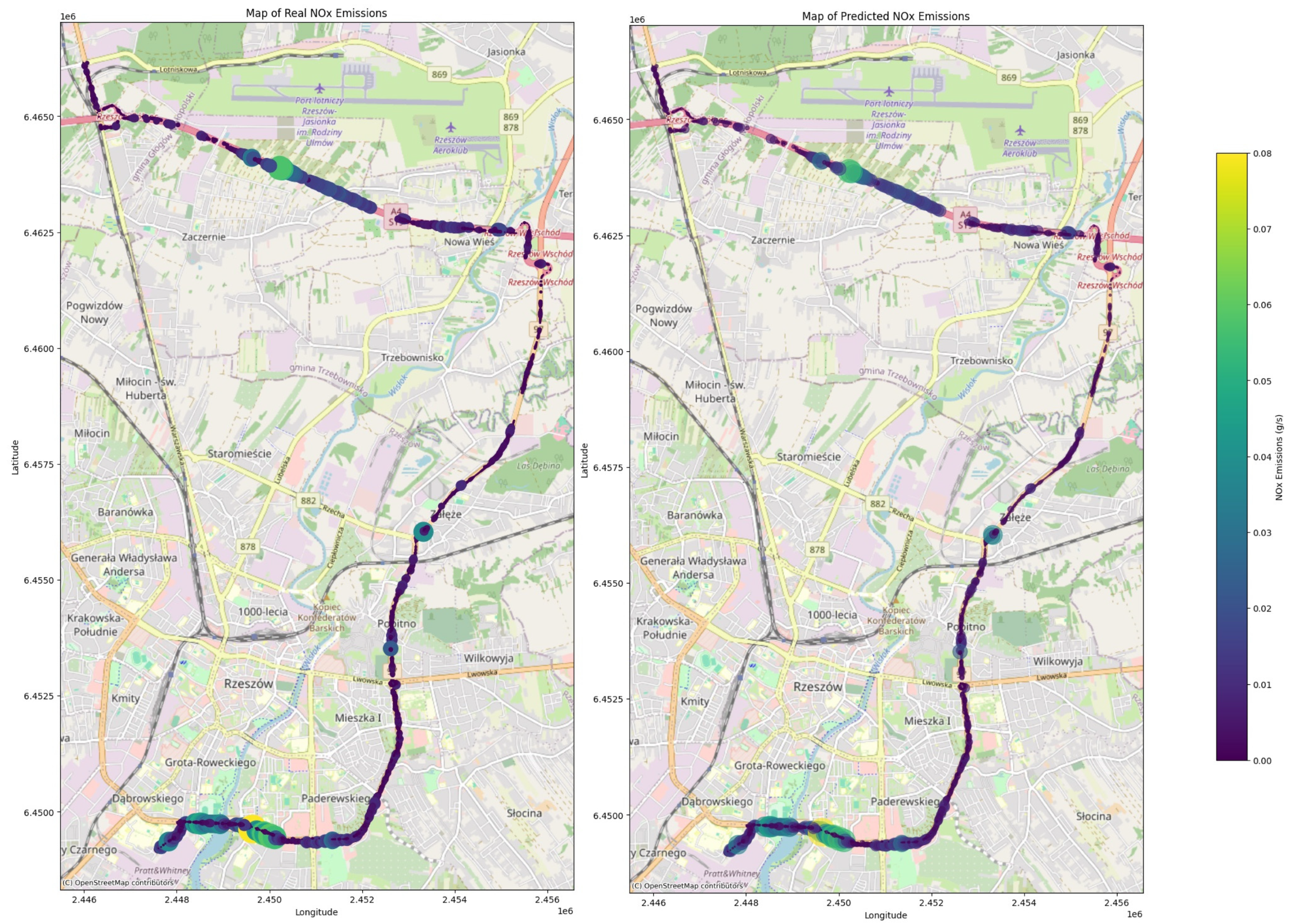
The developed models can be used for new predictions simply by entering the variables V (velocity) and a (acceleration). On the basis of these inputs, emissions can be predicted for selected engine operating conditions: cold or hot. These models are applicable to new real-world data, which can be easily obtained from road tests using tools such as smartphones and GPS. They can also be used for computer simulations, for example, by generating vehicle movement data from simulation software such as Vissim. The models generate emission data in grams per second (g/s) or as the total emissions of the entire test route. If vehicle location data are available, it is also possible to generate emission maps.
An example of NOx emission map generation, using both real and predicted data, is presented in Figure 8. For the developed models, it is possible to adjust the engine warm-up time so that the model initially estimates emissions for a cold engine and, after a certain period, switches to estimating emissions for a hot engine. Based on Figure 8, it can be observed that for each stage of driving with new road data, the model estimates NOx emissions with very good precision.

4. Discussion

In the context of modeling emissions from older vehicles, research reveals significant gaps in the existing literature, highlighting the need for further studies and innovations. Analysis of previous work shows a tendency to focus on modeling individual pollutants, such as CO2, NOx, or CO, without considering their collective characteristics. This study addresses this gap by presenting an approach that models emissions as a group of components, contributing to a more comprehensive and accurate understanding of emissions from older vehicles.
Furthermore, existing research often focuses on specific vehicle fueling technologies, such as LPG or CNG, without considering the impact of vehicle age on emissions [60,61]. This study expands this scope by incorporating aging vehicles as a critical element of emissions analysis, allowing models to better adapt to real-world operating conditions.
Another important aspect is the use of clustering techniques in the modeling process. Previous studies have not addressed this topic, which is a notable limitation. This research introduces an innovative approach by clustering input data, significantly enhancing the predictive capabilities of emission models. Emissions were classified into two main groups: cold and hot engine conditions, enabling a more accurate representation of real-world operating conditions for older vehicles. This approach can be scaled to larger vehicle groups and emission databases, potentially leading to the development of more precise predictive models and more effective emissions management.
Achieving high R2 values for emissions such as THC and CO in the context of older vehicles presents significant challenges. The models developed in this study demonstrate that while R2 values may appear below the ideal threshold, typically around 0.9, this reflects the complex interplay of various factors that influence emissions. In addition to the chosen explanatory variables, factors such as catalytic converter efficiency, combustion chamber temperature, throttle operation, and fuel injection control play crucial roles in emission formation. Despite the lower R2 values observed, the models still provide valuable information on emissions derived from road tests, indicating that they can reliably replicate emissions data from vehicle operation. Thus, even with R2 values of 0.74, 0.59, and 0.48, the models contribute meaningful findings to understanding and managing emissions from aging vehicle fleets, showcasing their potential to inform transportation policy and pollution reduction strategies. It is also worth noting the analysis of data inconsistencies. In any emission modeling study, the quality and reliability of the input data are paramount. The uncertainties inherent in the data collected from road tests and the On-Board Diagnostics II (OBDII) interface can significantly influence the accuracy of the emission estimates [62]. Road tests may be subject to variability in driving conditions, including factors such as traffic congestion, weather conditions, and driver behavior, all of which can lead to inconsistent measurements [63].
A relevant study to which the results of this research can be related is [64]. This work presents a methodology for creating models of THC and NOx emissions for vehicles with start-stop technology, considering the variability and dynamics of contemporary powertrains. Various machine learning techniques were tested, with random forests and gradient boosting demonstrating the best predictive capabilities, achieving an R2 of approximately 0.9 for engine emissions. Based on these results, recommendations for effective vehicle emission modeling were formulated. It is worth noting here that other computational techniques were used to create the models, and data clustering was not applied. Another study that highlights the application of machine learning techniques to vehicle-related issues is [65]. This article describes the process of creating an energy consumption model for electric vehicles (EVs), which allows for the rapid generation of results and the creation of energy maps. The best validation metrics were obtained using artificial intelligence methods, specifically neural networks, which enabled the development of two predictive models for the energy consumption of electric vehicles in winter and summer conditions, based on real driving cycles. Interesting findings on the emissions of vehicles with internal combustion engines and their continuous impact, especially on vehicle traffic in Poland, as well as the energy consumption of BEVs, are also presented in [66]. The article compares emissions from internal combustion engine vehicles (ICEVs) and battery electric vehicles (BEVs) in the context of Poland’s coal-based energy mix, accounting for air pollutant emissions such as CO2, NOx, SOx, CO, and particulate matter (TSP). The analysis shows that replacing internal combustion engine vehicles with electric vehicles in Poland is not beneficial, as while CO, CO2, and TSP emissions have decreased, NOx and SOx emissions have increased. The results are based on energy consumption data provided by the manufacturers and the COPERT model, as well as average vehicle mileage under Polish conditions. Aspects of emission modeling, particularly CO2, are also addressed in [67]. This work focuses on the development of accurate emission models for hybrid and electric vehicles, especially in the context of low-emission zones, where precise mobility planning requires simulations based on updated databases. The study presents a two-dimensional model of CO2 emissions for hybrid vehicles using artificial neural networks, which allows the simulation of various road scenarios and provides valuable information for future emission modeling work. The data for these models, unlike the models obtained in this work, do not present a split group of data for cold and warm exhaust emissions. The impact of fleet aging and its influence on modeling aspects is discussed in [68]. This study involves the development of a detailed inventory of air pollutant emissions from vehicles in Tianjin, a typical megacity in China, using a high-resolution time-space top-down method. The research found that light-duty passenger vehicles are the main sources of carbon monoxide and volatile organic compounds, while heavy-duty passenger and freight vehicles contribute significantly to nitrogen oxide and particulate matter emissions, with the majority of pollutants originating from vehicles meeting China III standards. Another paper that also uses vehicle motion data collected from OBD for mode-link emissions is [69]. The referenced study presents a parallel supervision system designed to accurately estimate vehicle CO2 emissions using OBD-independent information. It combines physical modeling with a modified long short-term memory (LSTM) neural network to create a robust framework capable of predicting emissions based on future road gradients and planned speed trajectories. The research emphasizes the importance of a cascaded structure and includes a deterioration factor to simulate aged vehicles, addressing the gap between regulatory test cycles and real-world carbon emissions. In contrast, this study primarily uses data from road tests and the OBDII diagnostic interface, focusing on a broader range of emissions, including CO2, CO, THC, and NOx. There are also a number of works that deal with finer scales of accuracy, such as meso and macro, for inputs such as average speed [70,71]. The work [70] addresses the critical issue of air pollution in urban areas, emphasizing the significant role of transportation systems in this challenge. It introduces a deep learning-based mesoscopic emission model that efficiently estimates CO2 and NOx emissions by leveraging extensive data from intelligent transportation systems. The model incorporates various vehicle attributes, average speeds, and road characteristics, showcasing its ability to provide accurate emissions estimates at the link level while balancing resource constraints and the need for resolution.
However, none of the aforementioned studies address the specifics of modeling older vehicles in detail. It is also important to note that the use of modern modeling techniques, leveraging artificial intelligence and Python programming in this study, has enabled the development of models that are well-suited to the characteristics of older vehicles. The application of machine learning algorithms, such as gradient boosting, allows one to capture complex emission patterns that would be difficult to determine using traditional methods. Consequently, these models offer more accurate emission forecasts and can support the development of emission reduction strategies, which is particularly relevant in the context of an aging vehicle fleet.
In light of this, future research should focus on further refining modeling methods, incorporating new analytical techniques, and expanding the range of input data. It is also essential to investigate the impact of various control technologies and fuels on older vehicle emissions to develop more comprehensive and adaptive emission management strategies.

5. Conclusions

This study presents a new methodology for modeling the exhaust emissions of older vehicles, integrating advanced artificial intelligence techniques and comprehensive data analysis from road tests. The findings demonstrate the effectiveness of the proposed approach in accurately predicting emissions, which is essential for forming transportation policies and emission reduction strategies, especially in the context of an aging vehicle fleet. Key findings include:
  • Development of predictive models for CO2, CO, THC, and NOx emissions using data clustering techniques and machine learning algorithms, notably gradient boosting.
  • Significant improvement in model accuracy through clustering of input data, enhancing the ability to reflect emissions under various vehicle operating conditions.
  • Capability of the models to analyze exhaust emissions and generate emission maps for urban areas, providing critical insights for effective transportation planning.
  • Successful capture of complex emission patterns that traditional methods struggle to identify, showcasing the advantages of AI techniques.
  • Affirmation of the effectiveness of the methodology in modeling emissions from older vehicles, offering valuable insights for decision-makers in environmental analysis and transport planning.
Future research can build on this study by expanding the methodology to include various vehicle types, such as hybrid vehicles, which will provide a more comprehensive understanding of their emission profiles. Additionally, the improvement and development of more advanced machine learning algorithms could improve predictive accuracy and computational efficiency. However, this study has limitations. The analysis is constrained by the availability and quality of the data from older vehicles, which may not capture the full diversity of vehicle conditions. Furthermore, the models developed may not fully account for all the variables that influence emissions, such as external environmental factors and specific driving behaviors. Focusing on CO2, CO, THC, and NOx may overlook other harmful emissions that affect air quality.

Funding

This research received no external funding.

Data Availability Statement

The data presented in this study are available on request from the corresponding author.

Conflicts of Interest

The authors declare no conflicts of interest.

Abbreviations

AIArtificial Intelligence
COCarbon monoxide
CO2Carbon dioxide
CNGCompressed natural gas
EVElectric vehicle
ICEVInternal combustion engine vehicles
LPGLiquified petroleum gas
MAEMean Absolute Error
MSEMean squared error
NNETNeural network
NOxNitrogen oxides
PEMSPortable Emission Measurement System
PHEVPlug-in hybrid electric vehicle
PMParticulate matter
R2Coefficient of determination
RMSERoot mean square error
SOxSulfur Oxide
SVMSupport vector machine
THCTotal hydrocarbons

References

  1. Agamloh, E.; Von Jouanne, A.; Yokochi, A. An overview of electric machine trends in modern electric vehicles. Machines 2020, 8, 20. [Google Scholar] [CrossRef]
  2. Suarez-Bertoa, R.; Selleri, T.; Gioria, R.; Melas, A.D.; Ferrarese, C.; Franzetti, J.; Arlitt, B.; Nagura, N.; Hanada, T.; Giechaskiel, B. Real-time measurements of formaldehyde emissions from modern vehicles. Energies 2022, 15, 7680. [Google Scholar] [CrossRef]
  3. Sharma, R.; Kumar, R.; Singh, P.K.; Raboaca, M.S.; Felseghi, R.A. A systematic study on the analysis of the emission of CO, CO2 and HC for four-wheelers and its impact on the sustainable ecosystem. Sustainability 2020, 12, 6707. [Google Scholar] [CrossRef]
  4. Mądziel, M.; Campisi, T. Investigation of Vehicular Pollutant Emissions at 4-Arm Intersections for the Improvement of Integrated Actions in the Sustainable Urban Mobility Plans (SUMPs). Sustainability 2023, 15, 1860. [Google Scholar] [CrossRef]
  5. Jaworski, A.; Mądziel, M.; Lew, K.; Campisi, T.; Woś, P.; Kuszewski, H.; Wojewoda, P.; Ustrzycki, A.; Balawender, K.; Jakubowski, M. Evaluation of the Effect of Chassis Dynamometer Load Setting on CO2 Emissions and Energy Demand of a Full Hybrid Vehicle. Energies 2022, 15, 122. [Google Scholar] [CrossRef]
  6. Shepelev, V.; Glushkov, A.; Slobodin, I.; Cherkassov, Y. Measuring and modelling the concentration of vehicle-related PM2.5 and PM10 emissions based on neural networks. Mathematics 2023, 11, 1144. [Google Scholar] [CrossRef]
  7. Wallington, T.J.; Anderson, J.E.; Dolan, R.H.; Winkler, S.L. Vehicle emissions and urban air quality: 60 years of progress. Atmosphere 2022, 13, 650. [Google Scholar] [CrossRef]
  8. Park, J.; Shin, M.; Lee, J.; Lee, J. Estimating the effectiveness of vehicle emission regulations for reducing NOx from light-duty vehicles in Korea using on-road measurements. Sci. Total Environ. 2021, 767, 144250. [Google Scholar] [CrossRef]
  9. Jaworski, A.; Lejda, K.; Mądziel, M.; Ustrzycki, A. Assessment of the emission of harmful car exhaust components in real traffic conditions. IOP Conf. Ser. Mater. Sci. Eng. 2018, 421, 042031. [Google Scholar] [CrossRef]
  10. Vidyattama, Y.; Tanton, R.; Nakanishi, H. Investigating Australian households’ vehicle ownership and its relationship with emission tax policy options. Transp. Policy 2021, 114, 196–205. [Google Scholar] [CrossRef]
  11. Guttikunda, S.K. Vehicle Stock Numbers and Survival Functions for On-Road Exhaust Emissions Analysis in India: 1993–2018. Sustainability 2024, 16, 6298. [Google Scholar] [CrossRef]
  12. Gürbüz, H.; Şöhret, Y.; Ekici, S. Evaluating effects of the COVID-19 pandemic period on energy consumption and enviro-economic indicators of Turkish road transportation. In Energy Sources, Part A: Recovery, Utilization, and Environmental Effects; Taylor and Francis Group: Boca Raton, FL, USA, 2021; pp. 1–13. [Google Scholar]
  13. Ge, J.C.; Wu, G.; Yoo, B.O.; Choi, N.J. Effect of injection timing on combustion, emission and particle morphology of an old diesel engine fueled with ternary blends at low idling operations. Energy 2022, 253, 124150. [Google Scholar] [CrossRef]
  14. Gao, C.; Gao, C.; Song, K.; Xing, Y.; Chen, W. Vehicle emissions inventory in high spatial–temporal resolution and emission reduction strategy in Harbin-Changchun Megalopolis. Process Saf. Environ. Prot. 2020, 138, 236–245. [Google Scholar] [CrossRef]
  15. Alizadeh, H.; Sharifi, A. Analyzing urban travel behavior components in Tehran, Iran. Future Transp. 2023, 3, 236–253. [Google Scholar] [CrossRef]
  16. Gao, J.; Tian, G.; Sorniotti, A. On the emission reduction through the application of an electrically heated catalyst to a diesel vehicle. Energy Sci. Eng. 2019, 7, 2383–2397. [Google Scholar] [CrossRef]
  17. de Meij, A.; Astorga, C.; Thunis, P.; Crippa, M.; Guizzardi, D.; Pisoni, E.; Valverde, V.; Suarez-Bertoa, R.; Oreggioni, G.D.; Mahiques, O.; et al. Modelling the impact of the introduction of the EURO 6d-TEMP/6d regulation for light-duty vehicles on EU air quality. Appl. Sci. 2022, 12, 4257. [Google Scholar] [CrossRef]
  18. Xiao, C.; Chang, M.; Guo, P.; Chen, Q.; Tian, X. Comparison of the cost-effectiveness of eliminating high-polluting old vehicles and imposing driving restrictions to reduce vehicle emissions in Beijing. Transp. Res. Part D: Transp. Environ. 2019, 67, 291–302. [Google Scholar] [CrossRef]
  19. Singh, S.; Kulshrestha, M.J.; Rani, N.; Kumar, K.; Sharma, C.; Aswal, D.K. An overview of vehicular emission standards. Mapan 2023, 38, 241–263. [Google Scholar] [CrossRef]
  20. Zhan, T.; Ruehl, C.R.; Bishop, G.A.; Hosseini, S.; Collins, J.F.; Yoon, S.; Herner, J.D. An analysis of real-world exhaust emission control deterioration in the California light-duty gasoline vehicle fleet. Atmos. Environ. 2020, 220, 117107. [Google Scholar] [CrossRef]
  21. Jaworski, A.; Mądziel, M.; Kuszewski, H.; Lejda, K.; Balawender, K.; Jaremcio, M.; Jakubowski, M.; Wojewoda, P.; Lew, K.; Ustrzycki, A. Analysis of Cold Start Emission from Light Duty Vehicles Fueled with Gasoline and LPG for Selected Ambient Temperatures (No. 2020-01-2207); SAE Technical Paper: Warrendale, PA, USA, 2020. [Google Scholar]
  22. Guno, C.S.; Collera, A.A.; Agaton, C.B. Barriers and drivers of transition to sustainable public transport in the Philippines. World Electr. Veh. J. 2021, 12, 46. [Google Scholar] [CrossRef]
  23. Fullerton, D.; Gan, L. Cost-effective policies to reduce vehicle emissions. Am. Econ. Rev. 2005, 95, 300–304. [Google Scholar] [CrossRef]
  24. Qin, Y.; Liu, M.; Hao, W. Energy-optimal car-following model for connected automated vehicles considering traffic flow stability. Energy 2024, 298, 131333. [Google Scholar] [CrossRef]
  25. Le Cornec, C.M.; Molden, N.; van Reeuwijk, M.; Stettler, M.E. Modelling of instantaneous emissions from diesel vehicles with a special focus on NOx: Insights from machine learning techniques. Sci. Total Environ. 2020, 737, 139625. [Google Scholar] [CrossRef] [PubMed]
  26. Aliramezani, M.; Koch, C.R.; Shahbakhti, M. Modeling, diagnostics, optimization, and control of internal combustion engines via modern machine learning techniques: A review and future directions. Prog. Energy Combust. Sci. 2022, 88, 100967. [Google Scholar] [CrossRef]
  27. Giovannardi, E.; Brusa, A.; Petrone, B.; Cavina, N.; Tonelli, R.; Kitsopanidis, I. AI-Based Virtual Sensing of Gaseous Pollutant Emissions at the Tailpipe of a High-Performance Vehicle. SAE Int. J. Engines 2024, 17, 513–527. [Google Scholar] [CrossRef]
  28. Zhao, B.; Yu, L.; Wang, C.; Shuai, C.; Zhu, J.; Qu, S.; Taiebat, M.; Xu, M. Urban air pollution mapping using fleet vehicles as mobile monitors and machine learning. Environ. Sci. Technol. 2021, 55, 5579–5588. [Google Scholar] [CrossRef]
  29. Mądziel, M. Instantaneous CO2 emission modelling for a Euro 6 start-stop vehicle based on portable emission measurement system data and artificial intelligence methods. Environ. Sci. Pollut. Res. 2024, 31, 6944–6959. [Google Scholar] [CrossRef]
  30. Chen, J.; Dobbie, G.; Koh, Y.S.; Somervell, E.; Olivares, G. Vehicle emission prediction using remote sensing data and machine learning techniques. In Proceedings of the 33rd Annual ACM Symposium on Applied Computing, Pau, France, 9–13 April 2018; pp. 444–451. [Google Scholar]
  31. Hoang, A.T.; Nižetić, S.; Ong, H.C.; Tarelko, W.; Le, T.H.; Chau, M.Q.; Nguyen, X.P. A review on application of artificial neural network (ANN) for performance and emission characteristics of diesel engine fueled with biodiesel-based fuels. Sustain. Energy Technol. Assess. 2021, 47, 101416. [Google Scholar]
  32. Acheampong, A.O.; Boateng, E.B. Modelling carbon emission intensity: Application of artificial neural network. J. Clean. Prod. 2019, 225, 833–856. [Google Scholar] [CrossRef]
  33. Mądziel, M. Modelling CO2 Emissions from Vehicles Fuelled with Compressed Natural Gas Based on On-Road and Chassis Dynamometer Tests. Energies 2024, 17, 1850. [Google Scholar] [CrossRef]
  34. Mądziel, M. Liquified Petroleum Gas-Fuelled Vehicle CO2 Emission Modelling Based on Portable Emission Measurement System, On-Board Diagnostics Data, and Gradient-Boosting Machine Learning. Energies 2023, 16, 2754. [Google Scholar] [CrossRef]
  35. Liu, H.; Qi, L.; Liang, C.; Deng, F.; Man, H.; He, K. How aging process changes characteristics of vehicle emissions? A review. Crit. Rev. Environ. Sci. Technol. 2020, 50, 1796–1828. [Google Scholar] [CrossRef]
  36. Kadijk, G.; Elstgeest, M.; Vroom, Q.; Paalvast, M.; Ligterink, N.; van der Mark, P. On road emissions of 38 petrol vehicles with high mileages. TNO Rep. 2020, 8, 11883. [Google Scholar]
  37. Seo, J.; Park, J.; Park, J.; Park, S. Emission factor development for light-duty vehicles based on real-world emissions using emission map-based simulation. Environ. Pollut. 2021, 270, 116081. [Google Scholar] [CrossRef]
  38. Perugu, H. Emission modelling of light-duty vehicles in India using the revamped VSP-based MOVES model: The case study of Hyderabad. Transp. Res. Part D Transp. Environ. 2019, 68, 150–163. [Google Scholar] [CrossRef]
  39. Ziółkowski, A.; Fuć, P.; Lijewski, P.; Jagielski, A.; Bednarek, M.; Kusiak, W. Analysis of exhaust emissions from heavy-duty vehicles on different applications. Energies 2022, 15, 7886. [Google Scholar] [CrossRef]
  40. Pielecha, J.; Skobiej, K.; Gis, M.; Gis, W. Particle number emission from vehicles of various drives in the RDE tests. Energies 2022, 15, 6471. [Google Scholar] [CrossRef]
  41. Ziółkowski, A.; Fuć, P.; Lijewski, P.; Bednarek, M.; Jagielski, A.; Kusiak, W.; Igielska-Kalwat, J. The Influence of the Type and Condition of Road Surfaces on the Exhaust Emissions and Fuel Consumption in the Transport of Timber. Energies 2023, 16, 7257. [Google Scholar] [CrossRef]
  42. Andrych-Zalewska, M.; Chlopek, Z.; Merkisz, J.; Pielecha, J. Comparison of gasoline engine exhaust emissions of a passenger car through the WLTC and RDE Type Approval Tests. Energies 2022, 15, 8157. [Google Scholar] [CrossRef]
  43. Johary, R.; Révillion, C.; Catry, T.; Alexandre, C.; Mouquet, P.; Rakotoniaina, S.; Pennober, G.; Rakotondraompiana, S. Detection of large-scale floods using Google Earth Engine and Google Colab. Remote Sens. 2023, 15, 5368. [Google Scholar] [CrossRef]
  44. Li, Z. Forecasting weekly dengue cases by integrating google earth engine-based risk predictor generation and google colab-based deep learning modeling in fortaleza and the federal district, Brazil. Int. J. Environ. Res. Public Health 2022, 19, 13555. [Google Scholar] [CrossRef] [PubMed]
  45. Govender, P.; Sivakumar, V. Application of k-means and hierarchical clustering techniques for analysis of air pollution: A review (1980–2019). Atmos. Pollut. Res. 2020, 11, 40–56. [Google Scholar] [CrossRef]
  46. Scoccimarro, R.; Zaldarriaga, M.; Hui, L. Power spectrum correlations induced by nonlinear clustering. Astrophys. J. 1999, 527, 1. [Google Scholar] [CrossRef]
  47. Jia, H.; Ding, S.; Xu, X.; Nie, R. The latest research progress on spectral clustering. Neural Comput. Appl. 2014, 24, 1477–1486. [Google Scholar] [CrossRef]
  48. Teymoori, M.M.; Chitsaz, I.; Zarei, A. Three-way catalyst modeling and fuel switch optimization of a natural gas bi-fuel-powered vehicle. Fuel 2023, 341, 126979. [Google Scholar] [CrossRef]
  49. Hamedi, M.R.; Doustdar, O.; Tsolakis, A.; Hartland, J. Energy-efficient heating strategies of diesel oxidation catalyst for low emissions vehicles. Energy 2021, 230, 120819. [Google Scholar] [CrossRef]
  50. Prati, M.V.; Costagliola, M.A.; Zuccheroso, A.; Napolitano, P. Assessment of Euro 5 diesel vehicle NOx emissions by laboratory and track testing. Environ. Sci. Pollut. Res. 2019, 26, 10576–10586. [Google Scholar] [CrossRef]
  51. Hassan AA, H.; Shah, W.; Husein, A.M.; Talib, M.S.; Mohammed AA, J.; Iskandar, M. Clustering approach in wireless sensor networks based on K-means: Limitations and recommendations. Int. J. Recent Technol. Eng. 2019, 7, 119–126. [Google Scholar]
  52. Raykov, Y.P.; Boukouvalas, A.; Baig, F.; Little, M.A. What to do when K-means clustering fails: A simple yet principled alternative algorithm. PLoS ONE 2016, 11, e0162259. [Google Scholar] [CrossRef]
  53. Shutaywi, M.; Kachouie, N.N. Silhouette analysis for performance evaluation in machine learning with applications to clustering. Entropy 2021, 23, 759. [Google Scholar] [CrossRef]
  54. Ekemeyong Awong, L.E.; Zielinska, T. Comparative Analysis of the Clustering Quality in Self-Organizing Maps for Human Posture Classification. Sensors 2023, 23, 7925. [Google Scholar] [CrossRef] [PubMed]
  55. Kim, S.J.; Bae, S.J.; Jang, M.W. Linear regression machine learning algorithms for estimating reference evapotranspiration using limited climate data. Sustainability 2022, 14, 11674. [Google Scholar] [CrossRef]
  56. Lee, H.; Wang, J.; Leblon, B. Using linear regression, random forests, and support vector machine with unmanned aerial vehicle multispectral images to predict canopy nitrogen weight in corn. Remote Sens. 2020, 12, 2071. [Google Scholar] [CrossRef]
  57. Steigmann, L.; Di Gianfilippo, R.; Steigmann, M.; Wang, H.L. Classification based on extraction socket buccal bone morphology and related treatment decision tree. Materials 2022, 15, 733. [Google Scholar] [CrossRef]
  58. Huo, Z.; Zha, X.; Lu, M.; Ma, T.; Lu, Z. Prediction of carbon emission of the transportation sector in Jiangsu province-regression prediction model based on GA-SVM. Sustainability 2023, 15, 3631. [Google Scholar] [CrossRef]
  59. Petersen, A.H.; Ekstrøm, C. Technical Validation of Plot Designs by Use of Deep Learning. Am. Stat. 2024, 78, 220–228. [Google Scholar] [CrossRef]
  60. Jaworski, A.; Mądziel, M.; Kuszewski, H. Sustainable Public Transport Strategies—Decomposition of the Bus Fleet and Its Influence on the Decrease in Greenhouse Gas Emissions. Energies 2022, 15, 2238. [Google Scholar] [CrossRef]
  61. Wang, X.; Chen, L.-W.A.; Ho, K.-F.; Chan, C.S.; Zhang, Z.; Lee, S.-C.; Chow, J.C.; Watson, J.G. Comparison of vehicle emissions by EMFAC-HK model and tunnel measurement in Hong Kong. Atmos. Environ. 2021, 256, 118452. [Google Scholar] [CrossRef]
  62. Abdul-Manan, A.F. Uncertainty and differences in GHG emissions between electric and conventional gasoline vehicles with implications for transport policy making. Energy Policy 2015, 87, 1–7. [Google Scholar] [CrossRef]
  63. Tamayao, M.A.M.; Michalek, J.J.; Hendrickson, C.; Azevedo, I.M. Regional variability and uncertainty of electric vehicle life cycle CO2 emissions across the United States. Environ. Sci. Technol. 2015, 49, 8844–8855. [Google Scholar] [CrossRef]
  64. Mądziel, M. Quantifying Emissions in Vehicles Equipped with Energy-Saving Start–Stop Technology: THC and NOx Modeling Insights. Energies 2024, 17, 2815. [Google Scholar] [CrossRef]
  65. Mądziel, M. Energy Modeling for Electric Vehicles Based on Real Driving Cycles: An Artificial Intelligence Approach for Microscale Analyses. Energies 2024, 17, 1148. [Google Scholar] [CrossRef]
  66. Zimakowska-Laskowska, M.; Laskowski, P. Emission from Internal Combustion Engines and Battery Electric Vehicles: Case Study for Poland. Atmosphere 2022, 13, 401. [Google Scholar] [CrossRef]
  67. Mądziel, M. Future Cities Carbon Emission Models: Hybrid Vehicle Emission Modelling for Low-Emission Zones. Energies 2023, 16, 6928. [Google Scholar] [CrossRef]
  68. Sun, S.; Sun, L.; Liu, G.; Zou, C.; Wang, Y.; Wu, L.; Mao, H. Developing a vehicle emission inventory with high temporal-spatial resolution in Tianjin, China. Sci. Total Environ. 2021, 776, 145873. [Google Scholar] [CrossRef]
  69. Sun, Y.; Hu, Y.; Zhang, H.; Wang, F.; Chen, H. A Parallel Supervision System for Vehicle CO2 Emissions Based on OBD-Independent Information. IEEE Trans. Intell. Veh. 2022, 8, 2077–2087. [Google Scholar] [CrossRef]
  70. Dib, A.; Sciarretta, A.; Balac, M. Deep Learning-Based Mesoscopic Pollutant Emissions Modeling in Road Traffic Networks. In Proceedings of the 2024 IEEE Forum for Innovative Sustainable Transportation Systems (FISTS), Riverside, CA, USA, 26–28 February 2024; pp. 1–7. [Google Scholar]
  71. Matthias, V.; Bieser, J.; Mocanu, T.; Pregger, T.; Quante, M.; Ramacher, M.O.; Seum, S.; Winkler, C. Modelling road transport emissions in Germany–Current day situation and scenarios for 2040. Transp. Res. Part D Transp. Environ. 2020, 87, 102536. [Google Scholar] [CrossRef]
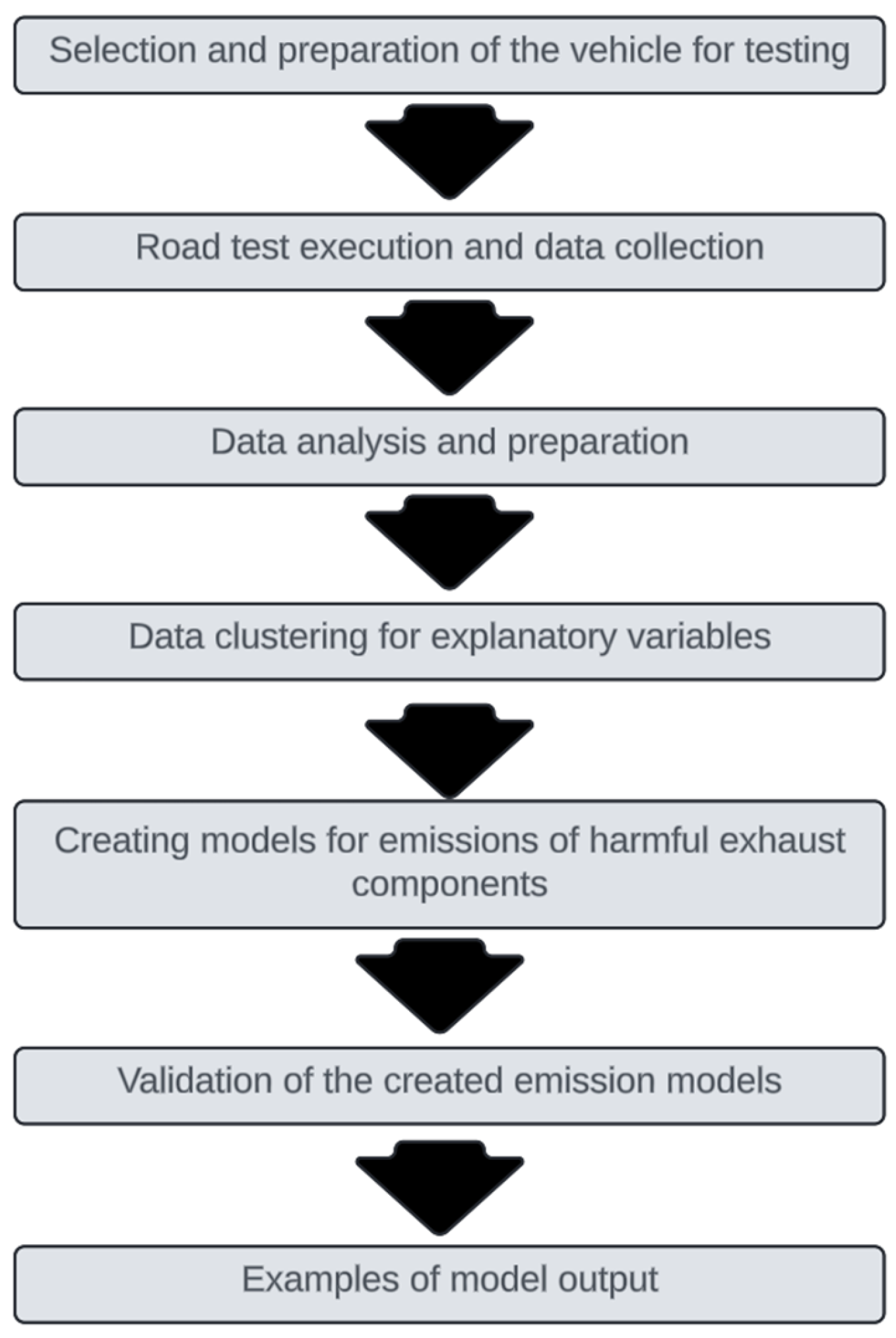
Figure 1. General scheme of work.
Energies 17 04924 g001
Figure 2. Scheme of the vehicle with connected devices.
Energies 17 04924 g002
Figure 3. General scheme for creating emission models.
Energies 17 04924 g003
Figure 4. Emissions of harmful exhaust components obtained during road tests.
Energies 17 04924 g004
Figure 5. Silhouette score results for finding the most optimal number of clusters.
Energies 17 04924 g005
Figure 6. Spectral Clustering for the data obtained for cold and hot emissions.
Energies 17 04924 g006
Figure 7. Example validation charts of THC prediction for a heated engine.
Energies 17 04924 g007
Figure 8. Example use of developed models for NOx prediction.
Energies 17 04924 g008
Table 1. Results of calculations of validation rates of MSE and R2 models for a given component of combustibles with an indication for the best prediction techniques.
Emission CompoundBest ModelMSE (± Std. Dev.)R2 (± Std. Dev.)
THC (Cold Engine)Random Forest Regression0.00003 ± 0.000010.756 ± 0.014
NOx (Cold Engine)Polynomial Regression0.00005 ± 0.000020.602 ± 0.013
CO (Cold Engine)Gradient Boosting Regression0.00288 ± 0.000150.485 ± 0.012
CO2 (Cold Engine)Polynomial Regression0.00319 ± 0.000100.926 ± 0.010
THC (Warm Engine)Gradient Boosting Regression0.00002 ± 0.000010.665 ± 0.013
NOx (Warm Engine)Polynomial Regression0.00002 ± 0.000010.424 ± 0.015
CO (Warm Engine)Polynomial Regression0.00275 ± 0.000140.225 ± 0.016
CO2 (Warm Engine)Polynomial Regression0.00219 ± 0.000090.954 ± 0.008
Disclaimer/Publisher’s Note: The statements, opinions and data contained in all publications are solely those of the individual author(s) and contributor(s) and not of MDPI and/or the editor(s). MDPI and/or the editor(s) disclaim responsibility for any injury to people or property resulting from any ideas, methods, instructions or products referred to in the content.