Predictive Artificial Intelligence Models for Energy Efficiency in Hybrid and Electric Vehicles: Analysis for Enna, Sicily

Abstract

Developments in artificial intelligence techniques allow for an improvement in sustainable mobility strategies with particular reference to energy consumption estimates of electric vehicles (EVs). This research proposes a vehicle energy model developed on the basis of deep neural network (DNN) technology. This study also explores the potential application of the model developed for the movement data of new vehicles in the province of Enna, Sicily, Italy, which are characterized by numerous attractors and the increasing number of hybrid and electric cars circulating. The energy model for electric vehicles shows high accuracy and versatility, requiring vehicle velocity and acceleration as input data to predict energy consumption. This research article also provides recommendations for the energy modeling of electric vehicles and outlines additional steps for model development. The implemented methodological approach and its results can be used by transport decision-makers to plan new transport policies in Italian cities aimed at optimizing vehicle charging infrastructure. They can also help vehicle users accurately estimate energy consumption, generate maps, and identify locations with the highest energy consumption.

1. Introduction

In recent years, the global automotive industry has undergone a profound transformation driven by increasing concerns about climate change and the need to reduce dependence on fossil fuels [1,2]. This shift towards sustainability has propelled electric vehicles (EVs) to the forefront of transportation innovation. Unlike traditional vehicles with internal combustion engines, which contribute significantly to greenhouse gas emissions and air pollution, electric vehicles offer a cleaner and more environmentally friendly mode of transportation [3,4]. The adoption of EVs represents a crucial step towards achieving global climate goals by eliminating emissions from internal combustion engines and reducing the overall carbon footprint [5,6]. This transition is not merely a technological substitution but symbolizes a broader social commitment to promote sustainable practices and ensure a cleaner and healthier future for generations to come [7,8].

Italy, renowned for its rich automotive heritage and engineering achievements, is at the forefront of the electric vehicle revolution. Taking advantage of a deeply rooted legacy in automotive innovation, from iconic sports cars to cutting-edge urban mobility solutions, Italy has unique opportunities to lead the adoption and advancement of electric vehicle technologies [9]. The country’s commitment to environmental conservation further underscores its readiness to embrace sustainable transportation alternatives. Italy’s largest automotive companies are currently rolling out a full range of vehicles utilizing 100% electric propulsion [10,11]. The growing demand for electric vehicles in Italy leads to the need to accurately understand and predict energy consumption patterns [12].

This is a topic not only related to innovative research purposes, but it is a basis for improving actions, strategies, and the choice of investments for energy and related management. In fact, a careful predictive analysis of the energy needs of EVs allows for better strategic planning related, for example, to the implementation of charging stations, to integrating renewable energy sources into the network, and to reducing the overall environmental impact of transport systems [13]. Developing predictive models of energy consumption also enables a better understanding of the operation of the vehicle for ordinary users, as these models should be accessible and user-friendly [14].

The issue of modeling energy consumption for hybrid and electric vehicles (EVs) is a complex issue that is gaining prominence in the context of global efforts to reduce greenhouse gas emissions and increase energy efficiency. Hybrid vehicles, which combine internal combustion and electric engines, as well as electric vehicles powered solely by electricity, require precise models to forecast energy consumption that account for various factors such as driving style, road conditions, and weather variability.

Artificial intelligence (AI), including machine learning and deep neural networks, plays a crucial role in the advancement of these models [15,16]. AI enables the analysis of vast amounts of vehicle-generated data, allowing the identification of consumption patterns and anomalies [17,18]. For example, machine learning models can predict fuel consumption and emissions in hybrid vehicles based on historical data and current operating conditions [19]. Similarly, for electric vehicles, AI can help optimize battery management and route planning, minimize energy consumption, and maximize vehicle range [20].

Modeling energy consumption and emissions using AI not only supports the development of more efficient and environmentally friendly vehicles, but it also allows better management of the energy grid. Precise forecasts of electric vehicle energy demand can help grid operators in load balance, the integration of renewable sources, and avoiding overloads. As a result, AI techniques contribute to the sustainable development of the transportation sector, while supporting the goals of environmental protection and energy efficiency.

Currently, efforts are underway to develop various models for electric vehicles (EVs), focusing on energy consumption during driving and optimizing charging infrastructure [21,22]. An example of this is [23]. This article presents a novel approach to modeling electric vehicles that integrates battery dynamics with vehicle dynamics and considers aerodynamic drag. The integrated battery electric vehicle (IBEV) model is titrated, and analyses demonstrate its superior energy efficiency compared to simplified models that neglect aerodynamic drag. To illustrate the utility of the proposed model, controllers were designed using linear quadratic integrator (LQI) regulators.

Another example is [24], which underscores the importance of optimal resource utilization in microgrids, examining systems with photovoltaic generators (PV), electric vehicles (EVs), electrical loads, and energy storage systems. Bidirectional power flow from the prosumers to the grid provides flexibility to manage excess energy generated or stored by the prosumers. Markov chain modeling was used to predict EV availability based on historical user travel data, incorporating PV power uncertainty.

Additionally, there is a growing body of work using artificial intelligence methods to model emissions and energy in vehicles. An example is [25], which introduces a methodology to measure and create a computational model of CO₂ emissions using artificial intelligence techniques for vehicles equipped with stop and start technology. This method relies on data from velocity, acceleration, and road gradients to predict CO₂ emissions. An analysis of three machine learning techniques revealed that gradient boosting achieved the best prediction results.

This article presents the development of a methodology for modeling energy consumption in electric vehicles (EVs). The methodology focuses on creating an accurate model for predicting energy consumption that is tailored to driving conditions within the city of Enna, Italy. This model was developed using deep neural networks (DNNs). The primary goal was to create a highly versatile model that could be used effectively by anyone. Therefore, only fundamental vehicle motion parameters, such as velocity and acceleration, were selected as explanatory variables. The input of these parameters allows the model to generate energy consumption results for electric vehicles in kWh. These outcomes can facilitate better planning of charging infrastructure, optimizing charging schedules, and identifying locations with the highest energy consumption and potential for recovery.

In this way, vehicle users can plan more cost-effective charging sessions, such as when energy prices are lower, e.g., from photovoltaic panels. The model’s results can also estimate the precise cost of driving an EV in relation to energy prices. This article also explores the potential application of this model through a case study of driving conditions in Enna, Italy. On the basis of the motion data obtained for this area, sample energy consumption results for EVs were generated.

The novelty of this methodology lies in its reliance on just two key input data points: vehicle speed and acceleration, which can be easily obtained from GPS devices, such as smartphones, or traffic microsimulation models like PTV Vissim. These inputs were specifically chosen due to their universality and ease of access, making the model highly adaptable to various traffic environments. The ability to use simple, readily available data significantly broadens the potential applications of the model, enabling its use in both real-world and simulated traffic scenarios. Furthermore, this approach allows for the creation of a versatile and precise tool for energy consumption estimation. The model’s high accuracy makes it valuable not only for analyzing microregional traffic patterns but also for optimizing infrastructure design, such as road networks, or developing traffic signal control strategies. These optimizations can lead to reduced energy consumption for vehicles or even enhanced energy recovery through regenerative braking, contributing to more sustainable transportation systems.

The topics and models discussed are crucial in shaping strategies for the development of energy and transportation in countries. Predictive models serve several critical functions. Primarily, they are essential for strategically locating the EV charging infrastructure to ensure availability and reliability in different parts of the country. They enable energy service providers to efficiently manage electric power demand, supporting grid stability and resilience in the midst of a growing number of electric vehicles on the roads.

Furthermore, these models are essential for policy makers and urban planners, helping them make informed decisions about investments in charging infrastructure, the development of public transportation, and the integration of renewable energy sources into the power grid. In the context of evolving energy and mobility landscapes, accurate forecasting of the energy consumption of electric vehicles is crucial to ensuring sustainable development, efficient resource management, and minimizing the environmental impact of transportation.

2. Methods

The general study workflow is described by two main steps, shown in Figure 1.

The first step involves developing a predictive model for EV energy consumption based on real-world data collected during road tests. These tests were carried out under conditions typical of the Enna region in Sicily, Italy, characterized by a relatively warm year-round climate with an average ambient temperature of 20.4 °C during the test sessions. The road tests lasted 200 min, using a Hatchback vehicle classified in segment B. Before the tests, the battery state of charge (SOC) was 80.1%, decreasing to 66.9% at the end of the test. The vehicle is equipped with a single electric motor that generates a total power of 125 kW and weighs 1390 kg. Its lithium-ion battery comprises 8 modules (96 cells connected in series) with a nominal capacity of 60 Ah. The vehicle has rear-wheel drive (RWD).

Data related to vehicle motion parameters and energy were recorded using a power analyzer at a frequency of 1 Hz. For model input, vehicle motion data such as velocity and acceleration were selected. This choice of explanatory variables ensures that the developed energy model can be universally applied to new road data, easily available through GPS tracking, or simulated vehicle motion data generated from software packages such as Simulink, Vissim, or SUMO. The variables used as response variables in the model are battery voltage and battery current, converted to energy units in kWh.

The collected data were subjected to an initial exploratory data analysis (EDA) to understand their distribution and potential patterns. Subsequently, the data were transformed, reformatted, and split into training sets. The training sets comprised 80% for training and 20% for testing purposes. The deep neural network (DNN) was chosen as the learning technique for the model. A DNN, also known as a deep neural network, is an advanced machine learning technique that mimics the structure of neurons in the human brain [26,27]. It consists of multiple layers of neurons, including hidden layers that process input data and transform them into predictions or classifications [28]. Each layer of neurons in a DNN is connected to every subsequent layer, allowing the network to recognize and extract complex patterns from the data [29]. The process of building a DNN model begins with determining the number of layers and neurons in each layer, followed by initializing random weights and biases that are gradually adjusted during the learning process [30]. The backpropagation algorithm plays a crucial role in optimizing the network parameters by minimizing the loss function based on comparisons between predictions and actual training data. The code used to create the model is presented in the following as Algorithm 1.

Algorithm 1. Fragment of the DNN model code used to create the energy model of electric vehicles

import tensorflow as tf from tensorflow.keras.models import Sequential from tensorflow.keras.layers import Dense, Dropout from tensorflow.keras.callbacks import EarlyStopping # Model creation DNN model = Sequential([   Dense(64, input_dim = 2, activation = ‘relu’),   Dropout(0.2),   Dense(32, activation = ‘relu’),   Dropout(0.2),   Dense(16, activation = ‘relu’),   Dense(1) ]) # Model compilation model.compile(optimizer = ‘adam’, loss = ‘mean_squared_error’) # Early stopping early_stopping = EarlyStopping(monitor = ‘val_loss’, patience = 10, restore_best_weights = True) # Model training history = model.fit(X_train_scaled, y_train, validation_split = 0.2, epochs = 100, batch_size = 32, callbacks = [early_stopping])

During the training of the DNN model, regularization techniques, such as dropout, were also applied to prevent overfitting. The first dense layer contains 64 neurons, takes input data of dimension 2, and uses the ReLU activation function, allowing for effective modeling of non-linear relationships in the data. A dropout layer with a dropout rate of 0.2 was added after the first layer to randomly exclude neurons during training, helping to reduce model overfitting. The next two dense layers have 32 and 16 neurons, respectively, also using the ReLU activation function, and the final layer has a single output neuron, making the model suitable for regression tasks.

The model was compiled using the Adam optimizer and the mean_squared_error loss function, which minimizes the mean squared error between the predicted and actual values. To prevent the model from overfitting the training data, early stopping was implemented. The EarlyStopping callback monitors the loss value on the validation set (val_loss), restoring the best weights of the model obtained during training if the loss value does not improve for 10 consecutive epochs.

The model training process with fit is performed on the training data X_train_scaled and y_train, with 20% of the data split for validation (validation_split = 0.2). The model is trained for 100 epochs with a batch size of 32. Using early stopping and monitoring the validation metric helps optimize the model, improving its ability to generalize to new data, and reducing prediction errors.

The model was created in Python within the Google Colab environment. Google Colab is a platform to create and run Jupyter notebooks in a web browser, providing free access to a virtual machine with computational resources, including CPUs and GPUs [31,32]. This is particularly useful for working with large data sets and machine learning algorithms [33].

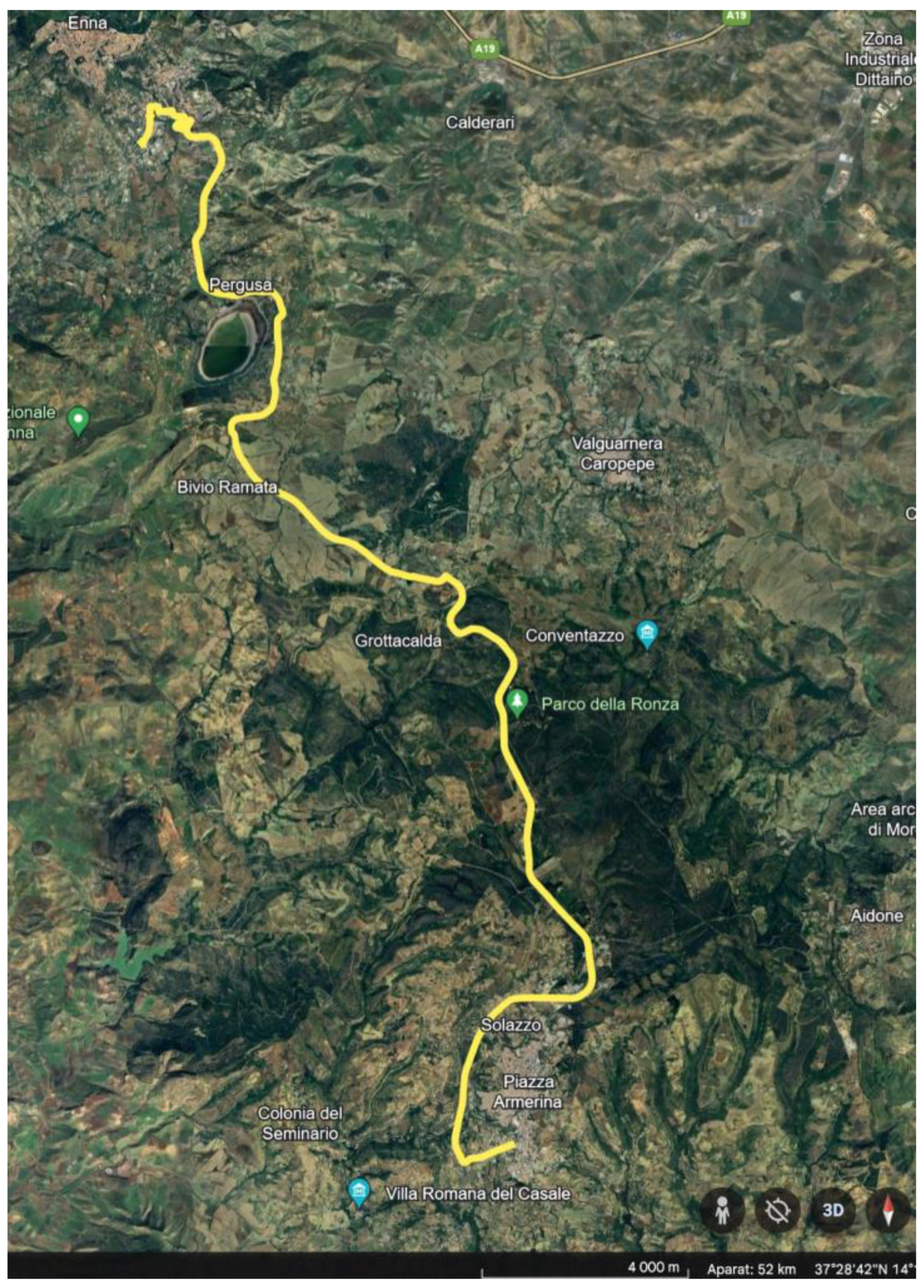
Next, to demonstrate the potential application of the energy model developed for electric vehicles, a new drive was recorded around the city of Enna and Piazza Armerina. The Enna and Piazza Armerina area, located in central Sicily, Italy, plays a significant role in regional transport. It features a well-developed road network that is crucial for local and regional mobility. The monitored transport infrastructure includes national main roads and local routes, enabling efficient travel by both private cars and public transport. Additionally, the region is important for tourism, influencing the development of the transport infrastructure and the demand for tailored transportation services for visitors. The route taken is shown in Figure 2.

The new journey undertaken is approximately 32 km long, with an average velocity of around 24 km/h. The route includes segments typical of urban, suburban, and high-speed expressway traffic. The testing of different traffic characteristics was crucial because electric vehicles exhibit a high energy recovery in urban areas, whereas energy consumption increases in places with high speeds and low regenerative braking, such as on roads. This choice of test route for the developed model is justified and should demonstrate the versatility of EV energy prediction for the developed model. Vehicle GPS data were recorded using a mobile GPS logger application. On the basis of this recording, a gpx file was generated, which can be used to produce new energy consumption results for the vehicle and to prepare an energy consumption map (the gpx file also contains vehicle movement coordinates). An application was prepared for easy extraction of vehicle traffic data from the gpx file, and its source code is presented in Algorithm 2.

Algorithm 2. Application code to convert the gpx file format to csv to collect input data for further energy analysis

import xml.etree.ElementTree as ET import csv def convert_gpx_to_csv(input_file, output_file):   tree = ET.parse(input_file)   root = tree.getroot()   # Define the namespaces   ns = {     ‘default’: ‘http://www.topografix.com/GPX/1/0’   }   # Prepare the CSV file   with open(output_file, ‘w’, newline=”) as csvfile:     fieldnames = [‘lat’, ‘lon’, ‘speed’]     writer = csv.DictWriter(csvfile, fieldnames = fieldnames)     writer.writeheader()     # Iterate over all track points     for trkpt in root.findall(‘.//default:trkpt’, ns):       lat = trkpt.get(‘lat’)       lon = trkpt.get(‘lon’)       speed_elem = trkpt.find(‘default:speed’, ns)       speed = speed_elem.text if speed_elem is not None else N’/A’       writer.writerow({         ‘lat’: lat,         ‘lon’: lon,         ‘speed’: speed       }) # Example usage convert_gpx_to_csv(input_file = “name of the file.gpx”, output_file = “output.csv”)

The code presented is a function that converts a GPX file to a CSV file, enabling the extraction of location and speed data stored in XML format. Initially, the necessary libraries are imported: xml.etree. ElementTree for XML parsing and csv for handling CSV data. The function convert_gpx_to_csv (input_file, output_file) starts by parsing the GPX file, reading the root of the XML tree, and defining the namespace to identify XML elements using their tags. Subsequently, a CSV file is prepared for data storage, specifying column headers, and initializing a csv.DictWriter object. Each track point (trkpt) in the GPX file is processed in a loop, collecting geographic data of latitude (lat), longitude (lon), and velocity. If velocity data are not available, it is assigned N/A. Finally, the data are written to the CSV file.

3. Results

In this chapter, the individual processes for obtaining results for the final acquisition of an EV energy model, which can be used for energy analysis under Italian conditions, will be presented.

First, exploratory data analysis (EDA) was performed to preliminarily verify and analyze the data. Subsequently, an electric vehicle energy model based on the deep neural network (DNN) technique was implemented in Python. This model was validated using metrics such as R², RMSE, MAE, MSE, and MAPE, and by analyzing graphs such as actual vs. predicted energy. Subsequently, energy analysis was performed for a new series of vehicle movement data on a route from Piazza Armerina to Enna in Italy. The entire process is summarized with recommendations for modeling such as EV energy models.

3.1. Exploratory Data Analysis

Exploratory data analysis (EDA) plays a crucial role in understanding the usage patterns, energy consumption, and performance of electric vehicles (EVs) [34,35]. EDA enables the identification and visualization of key variables such as vehicle velocity, acceleration, and energy consumption. When these data are analyzed, significant dependencies and correlations that impact the energy efficiency of electric vehicles can be uncovered. For example, analyzing speed and acceleration under different road conditions and their influence on energy consumption allows for the optimization of driving strategies and energy management. Geographic visualizations, such as vehicle route heat maps, can reveal areas with high energy consumption, highlighting the need for improved charging infrastructure in those locations. Additionally, EDA aids in detecting anomalies, such as unexpected increases in energy consumption, which may signal technical problems or improper vehicle usage. The distribution graphs for the variables analyzed are presented in Figure 3.

Based on Figure 3, we can observe histograms showing the frequency distribution of velocity, acceleration, and energy for the aggregated data ranges. The highest frequency of velocity data is observed in the first range, starting from 0 km/h to around 40 km/h. Similarly, the highest frequency of acceleration also resides around 0 km/h. The distribution of EV energy shows a wide spectrum of analysis, covering both consumed and regenerated energy.

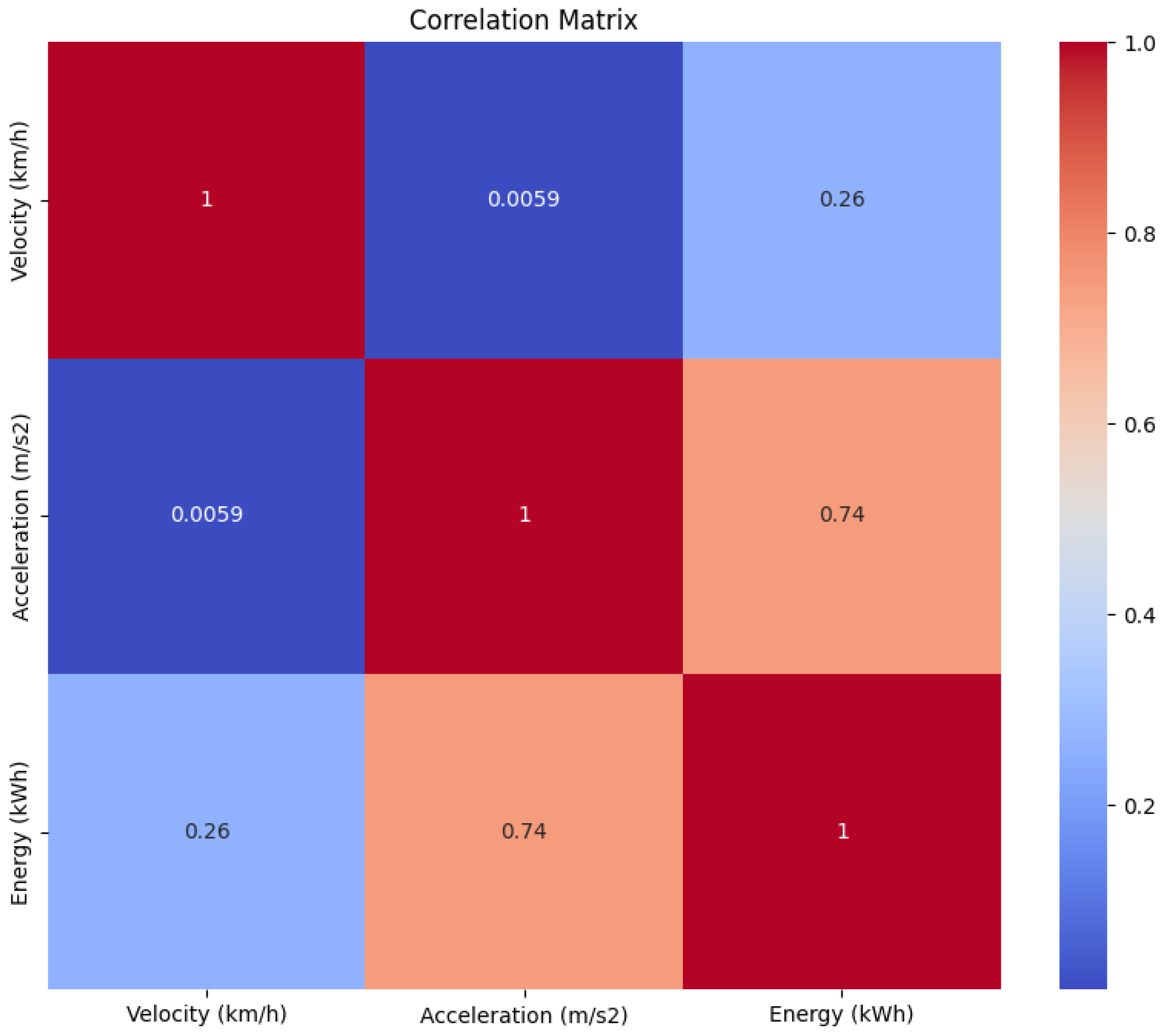
In the next step of EDA, a correlation matrix was generated for the explanatory variables and the dependent variable. A correlation matrix is a statistical tool used to understand the relationships between different variables in a data set [36]. The strength and direction of the linear relationship between two variables were measured. The results are shown in Figure 4.

Based on Figure 4, it can be observed that the dependent variable, which is energy, shows a strong correlation with the acceleration variable, making it the main factor influencing the precision of our model. The velocity variable also has some impact on energy consumption, but its correlation is significantly weaker compared to acceleration.

During the analysis of data related to energy consumption by EVs, proper data preparation for modeling is crucial. This process involves dividing the data into training and testing sets and scaling features, which is an essential step in ensuring the accuracy and efficiency of the model.

In this analysis, the data were divided into a feature matrix (X) containing vehicle velocity and acceleration variables (velocity (km/h) and acceleration (m/s²)), and a target variable (y) representing energy consumption (energy (kWh)). Subsequently, the data were split into training and testing sets using the train_test_split function from the scikit-learn library, where 80% of the data were allocated to the training set and 20% to the test set. This approach allows for evaluating the model’s performance on data that was not used for training, thereby increasing the reliability of the results. The code snippet that shows the execution of this step is presented in Algorithm 3.

Algorithm 3. Codesnippet on splitting the input data set to create an EV energy model

from sklearn.model_selection import train_test_split from sklearn.preprocessing import StandardScaler # Breakdown of data into features (X) and target variable (y) X = data[[‘Velocity (km/h)’, ‘Acceleration (m/s2)’]] y = data[‘Energy (kWh)’] # Division into training and test sets X_train, X_test, y_train, y_test = train_test_split(X, y, test_size = 0.2, random_state = 42)

Feature scaling is another crucial step that normalizes data to have a mean of 0 and a standard deviation of 1. This helps machine learning models trained on these data perform better and faster. The scaling process was conducted using StandardScaler, where the fit_transform function was applied to the training set and transformed to the test set to ensure consistency in scaling (Algorithm 4).

Algorithm 4. Codesnippet on feature scaling

# Feature scaling scaler = StandardScaler() X_train_scaled = scaler.fit_transform(X_train) X_test_scaled = scaler.transform(X_test)

3.2. Energy Modeling—Validation

The implementation and validation of a mathematical model for EV consumption has been defined. The description of the technique and the model itself was previously presented in Algorithm 1. This article showcased a deep neural network (DNN) built using the TensorFlow library, comprising dense and dropout layers, designed to predict the energy consumption of electric vehicles. The model was compiled with the ‘adam’ optimizer and ‘mean_squared_error’ loss function, then trained using early stopping to prevent overfitting. The training process involved splitting the data into training and validation sets and tuning hyperparameters over 100 epochs with a batch size of 32. To ensure the generalization capability of the deep neural network (DNN) model and prevent overfitting, several key techniques were employed during the training process. Early stopping was implemented to halt training when improvements in the validation set plateaued, thus preventing the model from continuing to adapt unnecessarily to the training data. Additionally, dropout layers were incorporated into the network architecture, introducing a form of regularization by randomly deactivating a fraction of neurons during training. This forces the model to learn more generalized features rather than memorizing specific patterns in the data.

Subsequently, the model was evaluated in the test set using loss functions, followed by generating predictions for this data set. For a thorough analysis of prediction results, various validation metrics were computed, such as mean absolute error (MAE), mean squared error (MSE), root mean squared error (RMSE), mean absolute percentage error (MAPE), and coefficient of determination (R²). Furthermore, the prediction results were visualized using a scatter plot of actual vs. predicted energy consumption values, allowing an assessment of model accuracy. The distribution of prediction errors was illustrated with a histogram, which facilitated the identification of potential deviations.

Evaluation of the deep neural network (DNN) model to predict the energy consumption of electric vehicles (EVs) demonstrated high precision. The mean absolute error (MAE) was 0.0008, indicating a minimal deviation of the predicted values from the actual values. The mean square error (MSE) achieved a value of 0.000002, suggesting a very small difference between the predictions and the actual values. The root mean square error (RMSE) was 0.0014, confirming the high accuracy of the model. The mean absolute percentage error (MAPE) was 1.24%, indicating small percentage differences between the predicted and actual energy consumption values. The coefficient of determination (R²) reached 0.91, indicating a very strong fit of the model to the test data and a high effectiveness in explaining the variability of the energy consumption of electric vehicles. These results clearly demonstrate that the proposed DNN model is highly precise and efficient in predicting energy consumption, making it a valuable tool for the analysis and optimization of the energy use of electric vehicles.

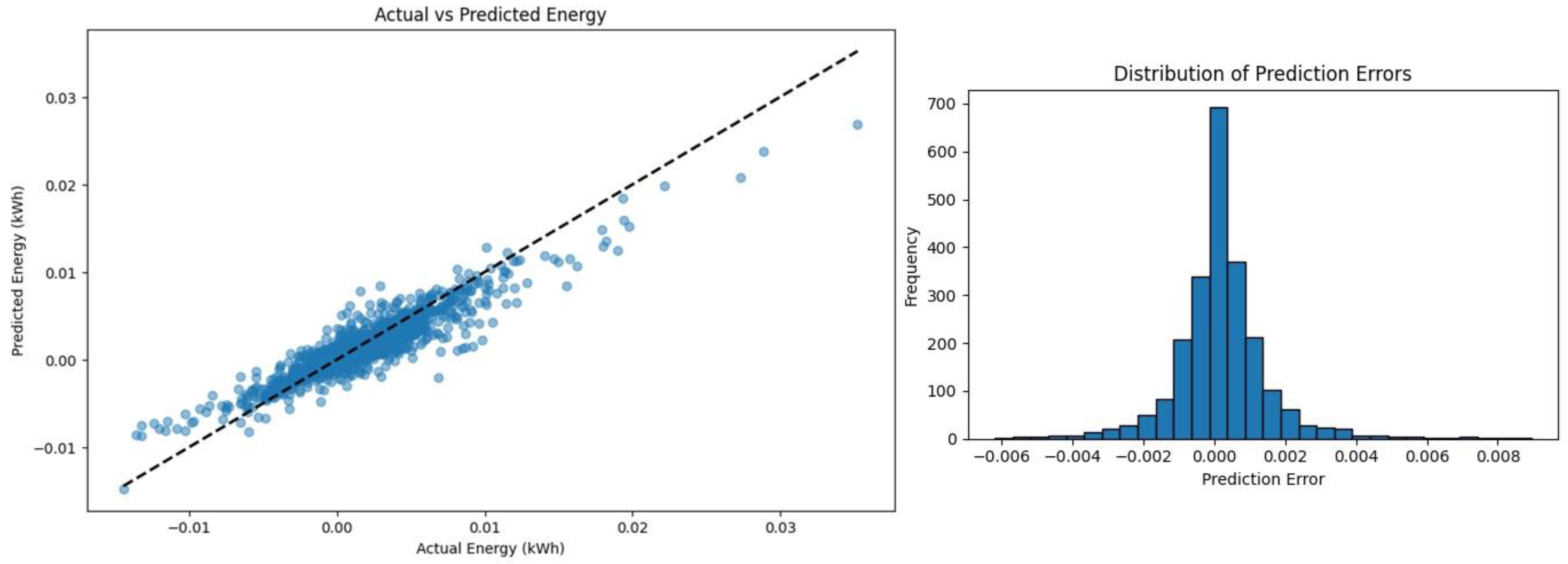
The results for the scatter plot of actual vs. predicted data and the distribution of prediction errors are shown in Figure 5.

The actual vs. predicted plot is a crucial tool for visually assessing the performance of a predictive model. The horizontal axis of the plot shows the actual values of the target variable (in this case, energy consumption in kWh), while the vertical axis shows the values predicted by the model. Ideally, the points on the plot should align along a straight line with a 45-degree angle, indicating perfect model fit; each predicted value matches exactly the actual value. Based on Figure 5, there is a notable clustering of points around the perfect prediction line, indicating the high accuracy of the energy model. The trend of the points resembles a straight line.

The distribution of the prediction error plot, also visible in Figure 5, is used to analyze the distribution of prediction errors made by the model. This focuses on the difference between actual and predicted values, allowing for an assessment of prediction accuracy and error distribution. The distribution of errors also indicates a well-developed model, since most errors are centered around 0, indicating that the model tends to overestimate and underestimate to a similar extent. The histogram itself resembles a normal distribution curve, indicating that most errors are small, with only a few larger errors.

3.3. Using the Model for New Input Data—Case Study of Enna

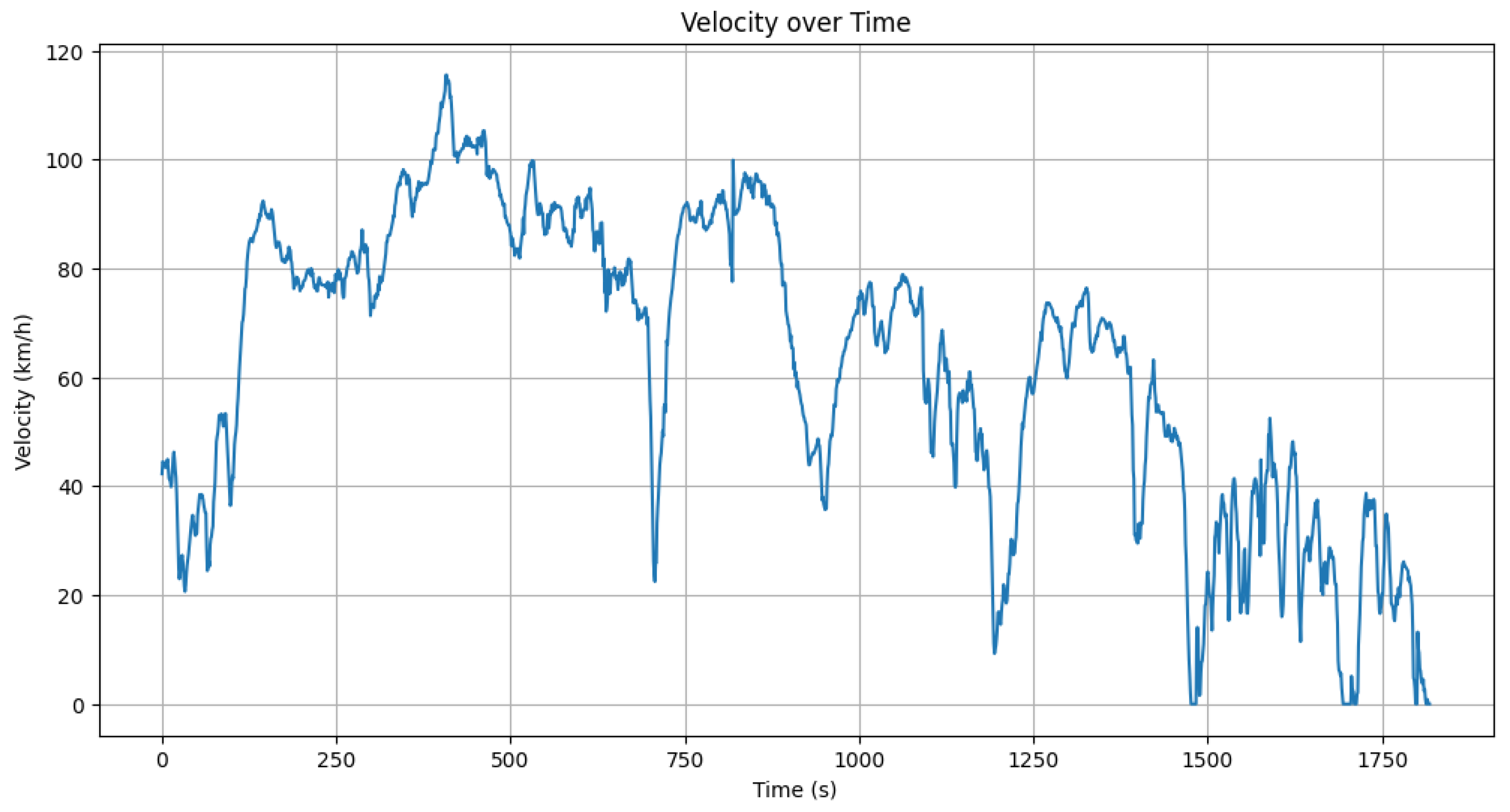
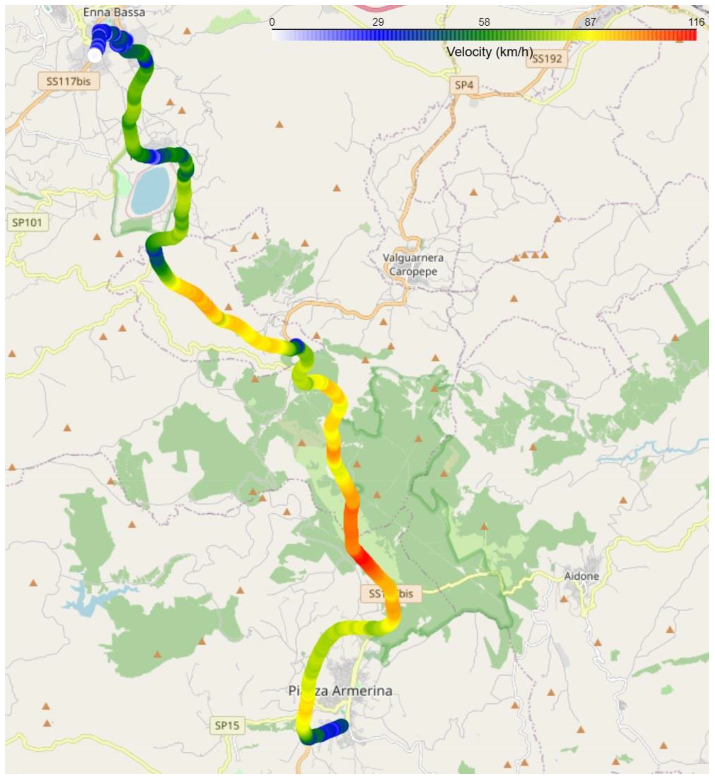
Next, to potentially demonstrate the utility of the energy model for driving conditions in the Enna area of Italy, a new journey was recorded. Subsequently, these data were used to generate new energy data for an electric vehicle. The velocity profile for the recorded journey is shown in Figure 6.

The new route included passages through sections with varying speed characteristics, as evident from the speed profile obtained. The objective of the trip was to cover urban areas characterized by lower speeds and frequent start–stop operations, as well as suburban and highway sections where the vehicle travels at higher speeds with fewer braking operations, resulting in increased energy consumption. Obtaining such a speed profile should allow for testing of the model’s prediction accuracy across different road conditions and speed ranges.

The velocity achieved on the analyzed route was visualized using the recorded geographic coordinates of the vehicle in the form of a point map (Figure 7).

The earlier discussion is corroborated by Figure 7, where distinctly lower speeds are observed during passages through city centers, acceleration in suburban areas, and higher speeds on highways. This distribution of speeds provides good input data for further analysis and validation of the developed EV energy model.

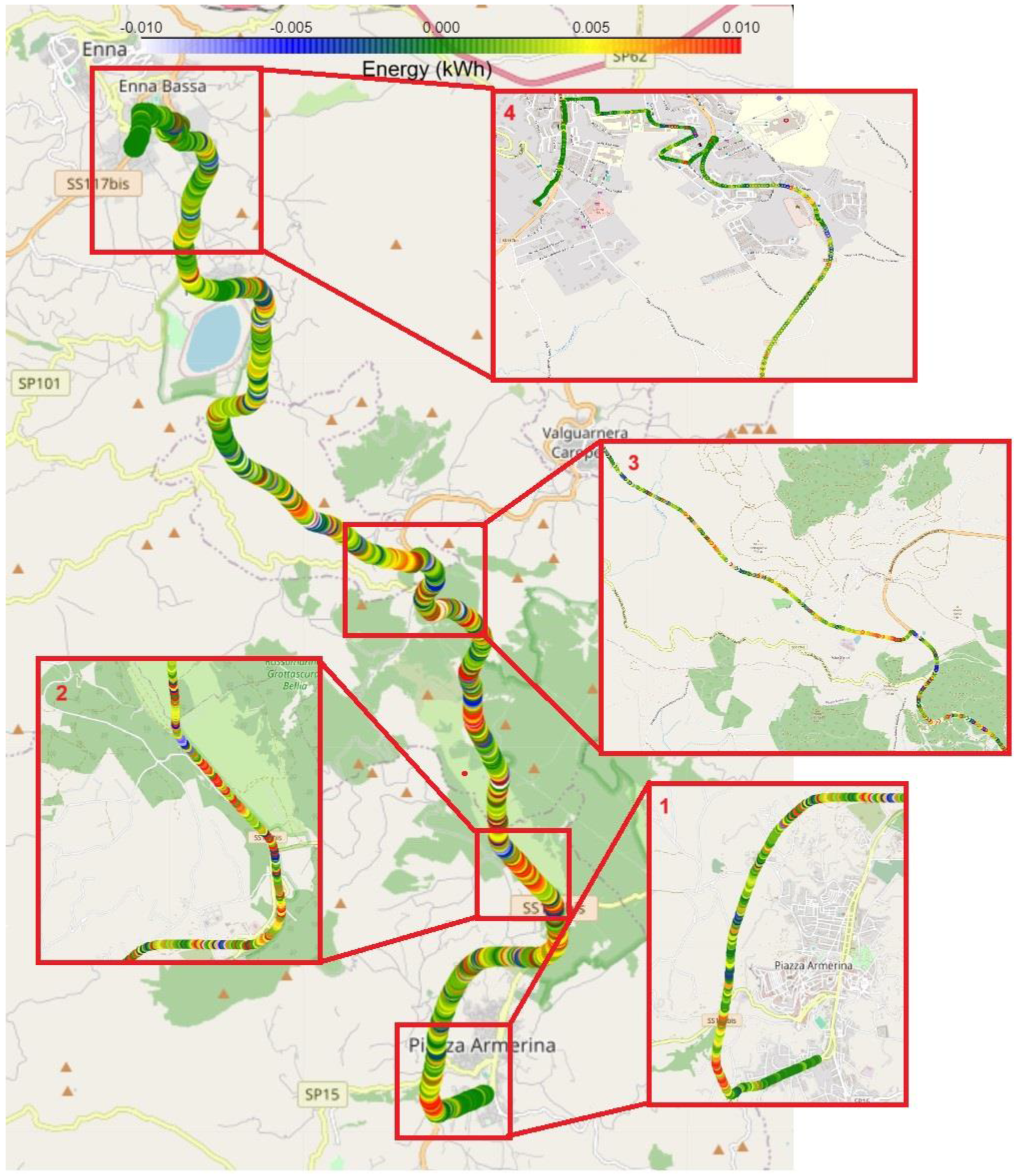
The input speed data recorded at the 1 Hz frequency were also converted into vehicle acceleration data, forming a comprehensive data set to generate energy results for the analyzed route. The complete energy map generated from the developed model is presented in Figure 8.

Based on Figure 8, we can observe the route with marked points that indicate energy consumption. This map was created to reflect different driving characteristics, including urban traffic and highways. On the basis of the developed map, we can identify areas where the EV experiences increased energy consumption and where regenerative braking occurs. Certain sections of this route have been zoomed in and presented in detail. For example, Area 1 in Figure 8 covers the driving area on Piazza Armerina, where we can observe rapid accelerations (such as from traffic lights) and braking due to dense traffic and pedestrian crossings, resulting in energy recovery through regenerative braking.

For Area 2 in Figure 8, we observe moments of high energy consumption due to frequent acceleration events at higher speeds. Similarly, for Area 4, we see urban driving where energy consumption is relatively low because the vehicle operates in a city environment in Enna.

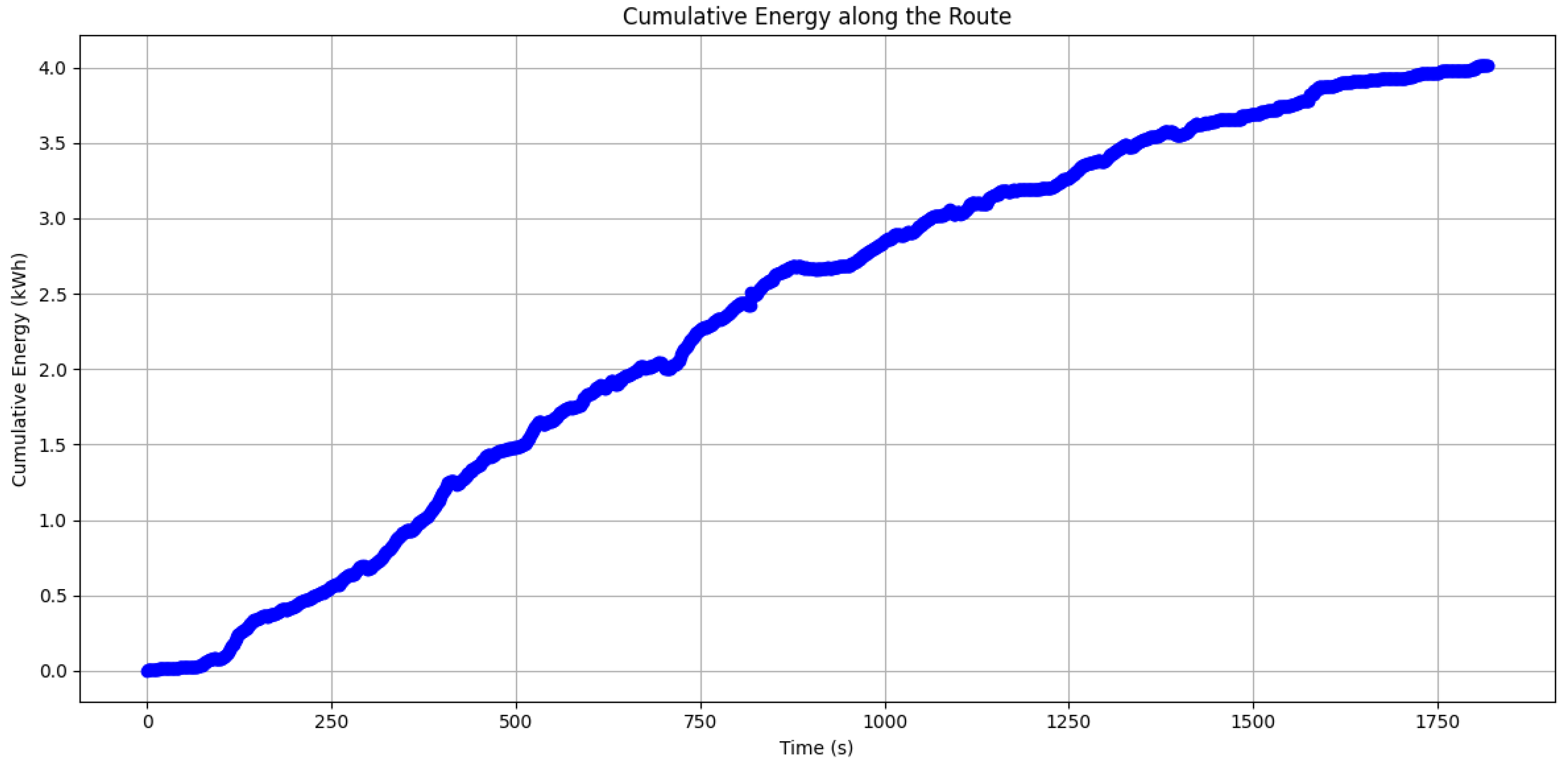
Based on the generated EV energy results, the developed model also allows the generation of a cumulative energy plot (Figure 9). From this graph, we can observe periods of increases in dynamic energy consumption. The vehicle consumed approximately 4 kWh of energy throughout the segment of the route.

3.4. Recommendations for Modeling EV Energy

Based on the methodology developed for measuring electric vehicle energy, processing road data, and developing and using an electric vehicle energy model, several suggestions can be made for its preparation.

• It is important to collect road data for different road conditions and prevailing speeds, especially for urban and nonurban parts, where higher driving speeds occur.
• The DNN technique makes it possible to obtain very good validation indications both in terms of vehicle acceleration, where there is high energy consumption, and in moments of recuperative braking, where energy is recovered for vehicle batteries.
• For the creation of universal models, it is necessary to reduce the input data for their creation as much as possible, and for the movement of the vehicle it is best to be limited to the speed and acceleration of the vehicle, possibly taking into account the gradient of the terrain; such parameters are sufficient for the creation of predictive models of the energy of EVs and allow one to achieve good accurate models with high validation rates.
• It is also important for the generation of new results to have GPS post-arrival coordinates, which will allow the subsequent use of these coordinates for map generation, which can be very useful, for example, for transport decision-makers, or even for ordinary road users.
• Additionally, it is recommended to record speed and acceleration data at a frequency of 1 Hz. This frequency ensures a dense grid of energy consumption points along the studied route, enhancing the accuracy and detail of the energy consumption model.

4. Discussion

In this study, a deep neural network (DNN) model was developed to predict energy consumption in electric vehicles (EVs). The model was built using the TensorFlow library, employing dense and dropout layers to mitigate overfitting. After rigorous training and validation, the model demonstrated high precision and effectiveness in forecasting energy consumption under diverse driving conditions.

The validation phase yielded excellent results. These were MAE = 0.0008, MSE = 0.000002, RMSE = 0.0014, MAPE = 1.24%, R² = 0.91, confirming the high precision of the model in predicting energy consumption in electric vehicles. Subsequently, to explore the applicability of the model in new driving scenarios, a case study was conducted in the city of Enna, Italy. Using data from this journey, a new data set on energy consumption was generated. The route encompassed urban areas characterized by frequent start–stop operations, as well as suburban/highway sections where the vehicle traveled at higher speeds with fewer braking events.

Visual analysis of the speed profile along the route (Figure 7) provided crucial information to verify the model in different driving scenarios. Furthermore, using geographical coordinates, energy consumption patterns were mapped (Figure 8). This visualization revealed variations in energy usage across different segments of the road, which was pivotal for the further refinement and validation of our EV energy prediction model.

Detailed analysis of speed profiles and acceleration data, recorded at 1 Hz frequency, facilitated comprehensive energy calculations for the entire journey. The generated energy map highlighted areas of lower energy consumption, such as city centers with frequent accelerations, and higher consumption in suburbs characterized by sustained high speeds. It also pinpointed locations where regenerative braking effectively recovered energy, crucial for optimizing the performance and range of EVs.

The topic of modeling energy consumption in EVs spans a wide spectrum of studies, many of which employ artificial intelligence algorithms to predict various factors that influence the operation of electric vehicles. For example, one of these studies [37] analyzed the utilization of retired electric vehicle batteries (REVBs) in a hybrid PV–hydrogen–REVB energy system. The research presented an REVB model based on lithium battery capacity degradation, energy management strategy, and a multicriteria optimization model that encompasses energy loss minimization, system costs, and potential energy losses. Simulation results showed that ignoring REVB capacity degradation decreases system reliability, while applying the NSGA-II algorithm yielded superior optimization results.

Another example relevant to the modeling of battery parameters in electric vehicles is [38]. This article discusses the fundamentals of EV charging technology and battery modeling within this context, focusing on steady-state and dynamic modeling methods. The results highlighted the impact of fast charging on the efficiency of the energy cycle under both steady-state and dynamic conditions.

Another notable study addressed the modeling of energy consumption related to the operation of electric vehicle (EV) air conditioning systems in a warm climate [x]. The researchers developed a model to assess the impact of air conditioning on energy consumption in electric vehicles during two trips on a summer day: morning and afternoon. The results indicated a 2% increase in total energy consumption in the morning and a 10% increase in the afternoon due to air conditioning.

In a different approach, Ref. [39] focused on optimizing and predicting energy consumption in electric and hybrid vehicles using Markov chains. A key aspect of their research was developing a multiagent system (MAS) for real-time intelligent energy management from fuel cell (FC) and supercapacitor (SC) sources. They conducted simulations with online predictions, analyzed system responses for optimized power, and compared the results with those of other methods to determine the most effective energy management principles in hybrid electric vehicles (HEVs).

Furthermore, a study that included AI methods applied to charging infrastructure for EVs [40] introduced a novel approach to designing optimal energy systems for buildings. This work integrated machine learning models to predict EV charging demand, combining these data with building energy requirements simulated in EnergyPlus. Genetic algorithms and PROBID methods were then used to optimize total annual cost (TAC) and energy self-sufficiency indicators. The findings demonstrated that the demand for charging electric vehicles significantly impacts energy system design, particularly for smaller buildings, and offered insight into the development of future zero-emission building and transportation systems.

Another related work [41] analyzed and modeled the ‘Vehicle-to-Anything’ (V2A), exploring scenarios where electric vehicles serve as energy sources for electrical grids, buildings, or other vehicles. The researchers developed a universal mathematical model adaptable to various V2A applications in different locations, transforming the optimization problem into a nonlinear integer programming (INLP) format and proposing a solution method. Simulations confirmed the effectiveness of their approach, with results indicating substantial potential for cost reduction in energy consumption, achieving a 4.37% reduction in household energy expenses through the discharge of EV.

Similarly, focused on modeling energy consumption under climate and traffic conditions in Poland, Ref. [42] developed predictive models for EV energy consumption using neural networks. They created separate predictive models for winter and summer conditions based on real driving cycles. The validation indicators for summer conditions showed an R² of 86% and an MSE of 1.4, while for winter conditions, these were 89% and 2.8, respectively. Other examples of works that similarly describe the modeling methodology but are related to alternative fuels and their emissions are works [43,44,45].

This review of the literature and previous research in modeling vehicle operating parameters underscores the significant need for such methodologies. Discussions of related works illustrate the breadth of research in this field, but none have addressed the specific approach presented in this study. The methodology developed here is innovative and scalable for application in other regions of Italy and other types of electric vehicle.

The developed deep neural network (DNN) model serves as a significant tool for predicting energy consumption in electric vehicles under various driving conditions. Recommendations for future research emphasize the importance of collecting data during drives in various road conditions, focusing on velocity profiles and acceleration patterns. Simplifying the input parameters for velocity, acceleration, and terrain gradient ensures efficient model development and high prediction accuracy. Additionally, the use of GPS coordinates improves the utility of energy maps for transportation stakeholders and communities.

This work contributes to sustainable transport development by providing robust methodologies for energy modeling in electric vehicles, essential for informed decision-making and infrastructure planning. In the context of practical vehicle energy management systems, integrating a predictive algorithm into existing vehicle control frameworks is crucial for optimizing energy consumption in real-time scenarios. This algorithm can function as a module within the vehicle’s onboard computer system, continuously receiving and processing data from various sensors, such as speed, acceleration, battery status, and GPS for route information. By analyzing these inputs, the predictive model can provide real-time estimates of energy consumption, allowing for timely and informed decisions.

To enhance its effectiveness, the model can offer actionable recommendations to the driver based on the dynamic driving conditions and the specific characteristics of the planned route. For instance, if the algorithm predicts a steep incline ahead, it may suggest reducing speed or employing regenerative braking techniques to conserve energy. Additionally, the algorithm can monitor the driver’s behavior, providing feedback on how adjustments in driving style—such as smoother acceleration and braking—can further minimize energy usage.

Real-time data streams introduce unique challenges, necessitating the model’s ability to adapt to changing conditions and varying data quality. To address these challenges, a robust data preprocessing pipeline will be implemented, incorporating filtering techniques to reduce noise and anomaly detection algorithms to identify and manage outliers. This ensures that the predictions are accurate and reliable.

Moreover, integrating the model’s outputs with feedback control strategies can enhance energy management by providing real-time suggestions to the driver, thereby maximizing the vehicle’s operational range and efficiency. The successful integration of this predictive algorithm into vehicle energy management systems has the potential to significantly improve energy efficiency and extend the operational range of electric vehicles, contributing to a more sustainable transportation ecosystem.

To ensure the predictive model remains accurate and relevant over time, a systematic update and maintenance strategy will be implemented. This strategy will involve continuous data collection from the vehicle’s sensors and systems, encompassing energy consumption metrics, environmental factors, driver behavior, and vehicle performance data. Periodic model retraining will be scheduled at regular intervals, utilizing the newly collected data to refine the model’s parameters and enhance its predictive capabilities. Additionally, performance monitoring tools will be established to track the accuracy of predictions against actual energy consumption, helping to identify when the model’s performance degrades and indicating the need for retraining or adjustments. Integrating user feedback regarding the model’s recommendations and predictions will provide valuable insights into its practical applicability and highlight areas for improvement. Furthermore, exploring adaptive learning approaches will allow the model to update itself in real time based on incoming data streams, helping maintain accuracy without requiring extensive retraining sessions.

5. Conclusions

The development and validation of the deep neural network (DNN) model to predict energy consumption in EVs under various driving conditions yielded several significant results. The model demonstrated high precision and effectiveness, as evidenced by low prediction errors and a high coefficient of determination (R²). The key results of this study include a mean absolute error (MAE) of 0.0008 and a mean squared error (MSE) of 0.000002, indicating a minimal deviation of the predicted values from the actual values. The root mean squared error (RMSE) was 0.0014, which confirms the accuracy of the model in predicting EV energy consumption. The mean absolute percentage error (MAPE) was 1.24%, further highlighting the small differences between the predicted and actual energy consumption values.

A case study conducted in Enna, Italy, demonstrated the practical applicability of the developed model. Analysis of energy consumption differences across different road types and during various driving operations (start–stop, accelerations, regenerative braking) provided valuable insight for further model refinement and optimization of EV efficiency. The limitations of this study include the need to collect more data from various road conditions and integrate additional factors such as weather conditions and vehicle load, which can affect energy consumption. In addition, future research could focus on developing models that account for dynamic changes in driver behavior and electric vehicle technologies.

Development trends include further enhancement of predictive models to increase accuracy and adaptability to different driving scenarios. Advanced machine learning techniques such as recurrent neural networks and time-series modeling could also contribute to more precise forecasts of energy consumption in electric vehicles.