Article

Research on Anomaly Detection Model for Power Consumption Data Based on Time-Series Reconstruction

1
Longquan Power Supply Company, State Grid Zhejiang Electric Power Co., Ltd., Longquan 323799, China
2
School of Electronic and Information Engineering, Shanghai University of Electric Power, Shanghai 201306, China
*
Author to whom correspondence should be addressed.
Energies 2024, 17(19), 4810; https://doi.org/10.3390/en17194810
Submission received: 17 August 2024 / Revised: 16 September 2024 / Accepted: 24 September 2024 / Published: 26 September 2024
(This article belongs to the Section F1: Electrical Power System)

Abstract

:
The power consumption data in buildings can be viewed as a time series, where outliers indicate unreasonable energy usage patterns. Accurately detecting these outliers and improving energy management methods based on the findings can lead to energy savings. To detect outliers, an anomaly detection model based on time-series reconstruction, AF-GS-RandomForest, is proposed. This model comprises two modules: prediction and detection. The prediction module uses the Autoformer algorithm to build an accurate and robust predictive model for unstable nonlinear sequences, and calculates the model residuals based on the prediction results. Points with large residuals are considered outliers, as they significantly differ from the normal pattern. The detection module employs a random forest algorithm optimized by grid search to detect residuals and ultimately identify outliers. The algorithm’s accuracy and robustness were tested on public datasets, and it was applied to a power consumption dataset of an office building. Compared with commonly used algorithms, the proposed algorithm improved precision by 2.2%, recall by 12.1%, and F1 score by 7.7%, outperforming conventional anomaly detection algorithms.

1. Introduction

At present, the large-scale collection and storage of data has become a reality. Time-series data are widely prevalent in fields such as finance, weather forecasting, and health monitoring. However, within time-series data, there are often anomalies—data points that significantly deviate from the main pattern. These anomalies may be caused by various factors, such as sensor malfunctions or unexpected events. Consequently, the detection of outliers in time-series data is important.
Energy consumption data can be viewed as time series. Equipment failures or inefficient energy usage patterns can lead to abnormal energy consumption data. Implementing appropriate energy management measures to reduce the occurrence of such anomalies can effectively achieve energy savings. With the advancement in data collection and analysis technologies, algorithms for detecting anomalies in energy consumption data have rapidly evolved. From traditional statistical methods to machine learning-based approaches, various techniques have been proposed and applied specifically to anomaly detection in energy consumption data, providing support for energy management and optimization.
Classical time-series anomaly detection methods primarily include statistical-based anomaly detection algorithms, clustering and classification-based anomaly detection algorithms, and proximity-based anomaly detection algorithms. Statistical-based time-series anomaly detection algorithms encompass techniques such as the 3-sigma rule, quartile method, and other statistical measures. For instance, in Reference [1], a hyperspectral anomaly detection problem in remote sensing was addressed by treating third- and fourth-order matrices as statistical features to highlight anomalous peaks, making anomalies easier to detect. Reference [2] successfully employed the quartile method to identify wind-power anomaly data. Clustering-based anomaly detection methods are considered unsupervised learning techniques. For example, Reference [3] introduced an improved streaming K-means clustering algorithm designed for detecting abnormal electricity consumption behavior in large-scale power data streams, drawing inspiration from the CluStream streaming-data clustering algorithm. In Reference [4], model normality scores were first used to determine model clustering indices, with outliers identified based on these indices. Classification-based anomaly detection algorithms, on the other hand, can be viewed as supervised learning techniques. Reference [5], for example, proposed a method to measure the confidence of classification results, identifying outliers by constructing classifiers. Proximity-based anomaly detection methods mainly include density-based and distance-based approaches. Reference [6] preprocessed aggregated active power output and corresponding wind speed values, and then calculated weighted distances based on the similarity between each object in the data and the local outlier factor (LOF), to identify anomalies. Reference [7] proposed an improved LOF algorithm for detecting abnormal electricity consumption behavior in users.
Classical time-series anomaly detection methods are widely applied, but their effectiveness is limited when used on unstable, nonlinear, or multivariate time series. Energy consumption sequences are generally unstable and nonlinear [8]. In recent years, researchers have begun exploring deep learning-based methods for time-series anomaly detection, with significant attention given to methods based on prediction residuals (Residual = Actual Value − Predicted Value). For instance, in Reference [9], a study was conducted on a method that combines random forests with statistical algorithms for anomaly detection. The study first utilized a random forest algorithm to predict building energy consumption, followed by the application of an improved statistical algorithm to the prediction residuals for anomaly detection, demonstrating high detection accuracy. In Reference [10], the long short-term memory (LSTM) algorithm was used to predict energy consumption data, and anomaly scores were calculated based on the prediction results to ultimately identify anomalies. In reference [11], the GNN-GRU–Attention algorithm was used to model and predict energy-consumption time series, and an improved random forest algorithm was subsequently employed to detect anomalies in the residuals. Experimental results indicated that this approach outperformed other anomaly detection algorithms based on prediction residuals, as well as classical time-series anomaly detection methods. In Reference [12], a seasonal threshold approach was introduced to improve the accuracy of prediction-based outlier detection systems, especially for energy management systems in buildings. Reference [13] presents an AI-based anomaly detection method for electricity consumption in smart cities, using data from households in northeastern Mexico. It first predicts energy consumption with deep learning algorithms and then detects outliers by analyzing the residuals with the Isolation Forest algorithm.
The method of using deep learning algorithms to predict sequences, calculate residuals, and then analyze these residuals to identify anomalies can be considered a hybrid approach. The foundation of this approach lies in establishing highly accurate time-series prediction models. The data that significantly deviate from the predicted values can be identified as outliers. The advancement in deep learning technology has significantly enhanced the accuracy of prediction models, laying a solid foundation for the implementation of time-series anomaly detection algorithms based on prediction errors. In recent years, with the introduction of the Transformer algorithm [14], the accuracy and generalization capabilities of time-series prediction models have greatly improved. Building on this, the Informer [15] and Autoformer [16] algorithms have been proposed, making the model architecture more suitable for unstable and nonlinear time series.
This paper proposes a time-series anomaly detection model, AF-GS–RandomForest, based on the Autoformer algorithm. The model first employs the Autoformer algorithm to predict the time series, and then the residuals are analyzed using a random forest algorithm optimized through Grid Search (Grid Search, GS) parameter tuning. The accuracy and robustness of the algorithm were validated on public datasets, and the model was subsequently applied to detect abnormal energy consumption in an office building. The results demonstrated that the F1 score of the detection model reached 0.998, outperforming existing commonly used anomaly detection algorithms.

2. Algorithm Design

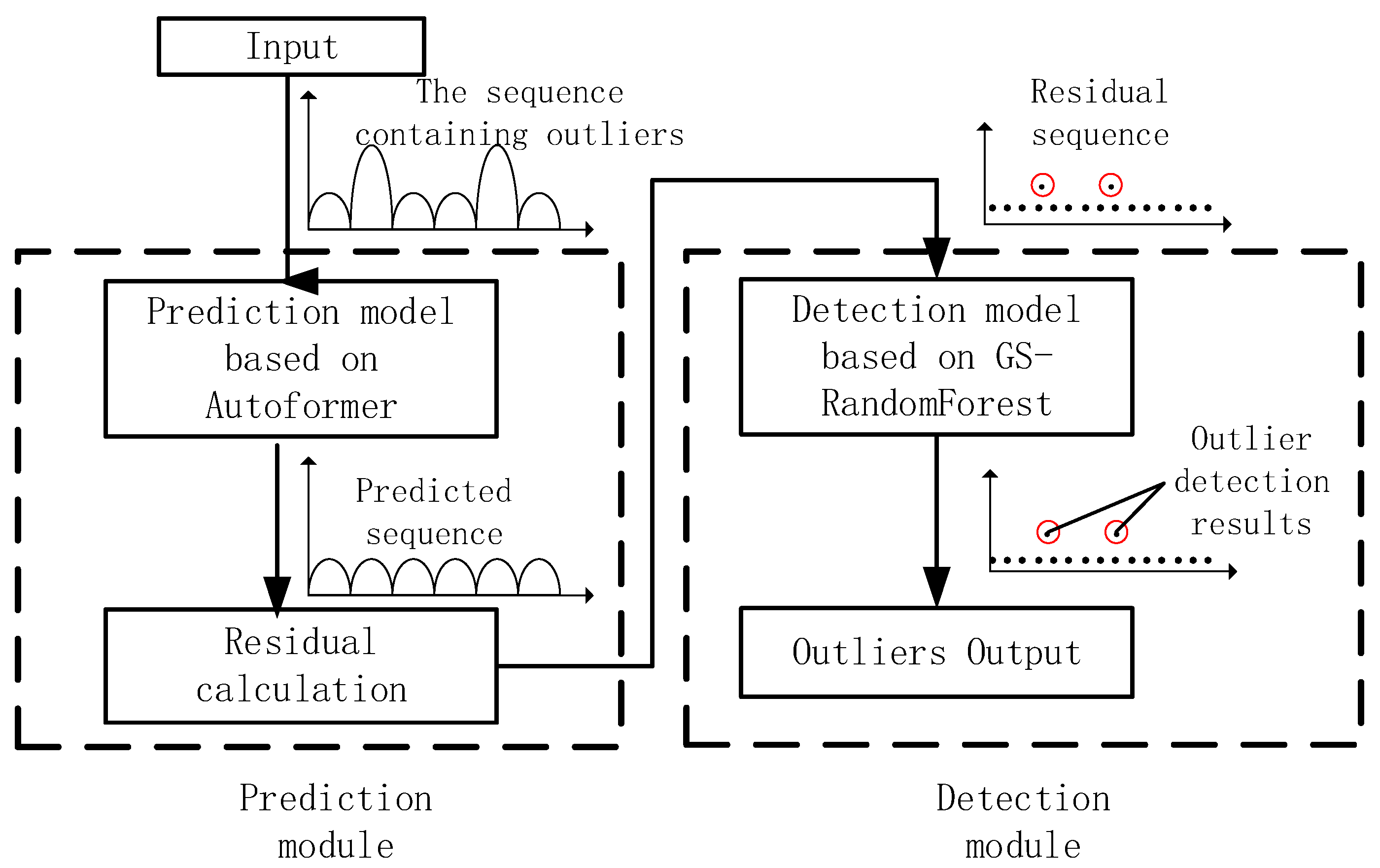
The structure of the AF-GS–RandomForest model consists of two components. The first component is the prediction module, which includes the sequence prediction and reconstruction module. This module employs the Autoformer algorithm to predict the time series and obtain the residuals. The second component detects anomalies in the residual sequence using the random forest algorithm optimized through Grid Search. The overall structure and workflow of the algorithm are illustrated in Figure 1, where a simple, univariate sequence without trends is used as an example to demonstrate the detection process.

2.1. Autoformer Algorithm

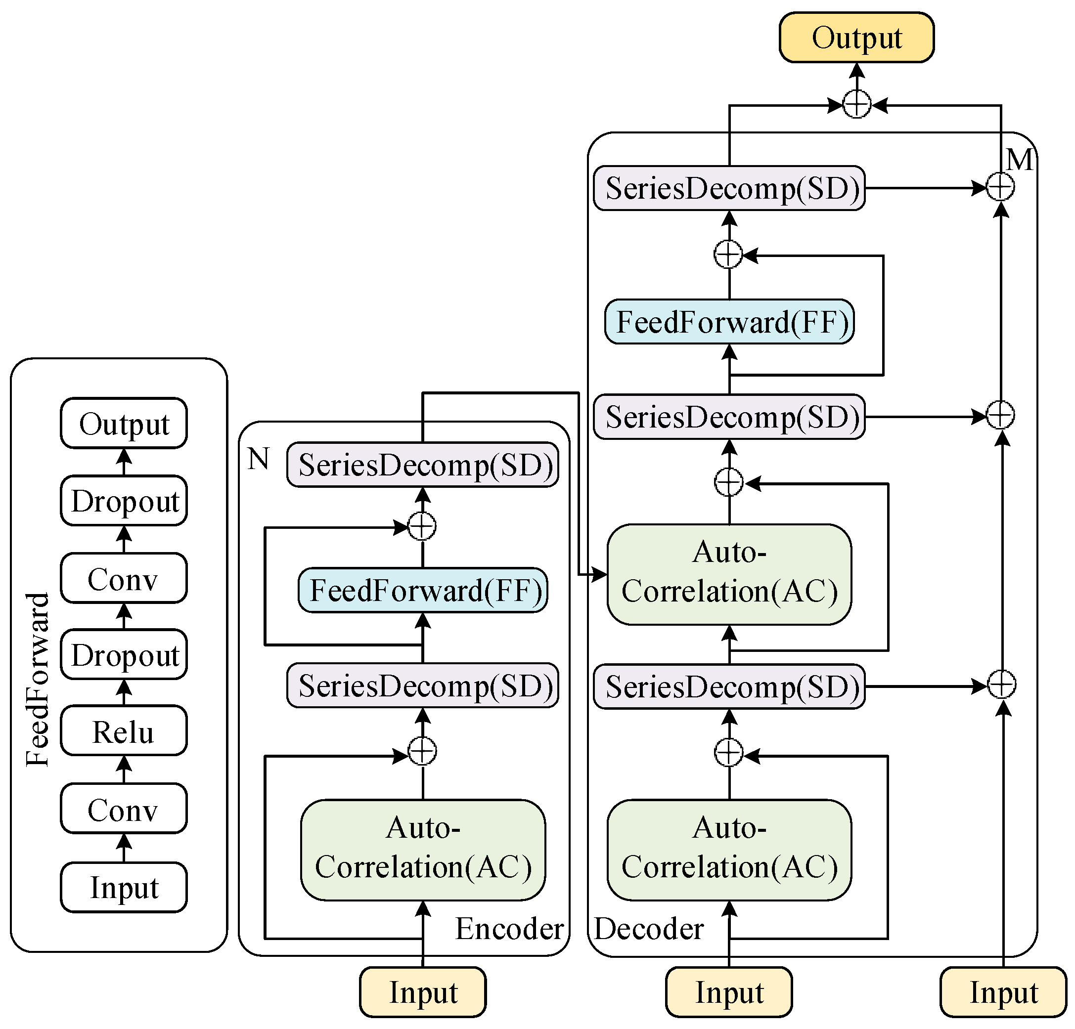
The structure of the time-series prediction model based on Autoformer is shown in Figure 2. As can be seen from the figure, the Autoformer algorithm is built around the encoder–decoder architecture, which integrates the processes of decomposition and auto-correlation for more accurate time-series predictions. The Decomposition Block gradually separates long-term trend information, while the auto-correlation mechanism identifies the similarity of subsequences based on the periodicity of the sequence, and aggregates similar subsequences. Since energy consumption sequences are typically long, often exhibit seasonal trends, and are closely related to human activity patterns, they possess subsequence similarity. Therefore, these modules of Autoformer enable the algorithm to achieve higher accuracy when predicting such sequences [16,17].
In detail, the input to the algorithm is a time-series sequence, which is first fed into the encoder. The encoder processes the input sequence N (the length of the input time series), decomposing it into trend and seasonal components. The Decomposition Block (SD) is responsible for this process, which is further enhanced by the auto-correlation (AC) mechanism that identifies and aggregates similar subsequences from different periods. This mechanism is crucial for handling periodic patterns in energy consumption data.
The processed output from the encoder is then passed to the decoder, which reconstructs the sequence into the final predicted output M (the length of the output sequence). The decoder applies similar steps by modeling the trend and seasonal components separately and combining them to produce the final predictions. The FeedForward (FF) layer further enhances the model’s ability to process the time series efficiently.
The encoder and decoder are connected by the decomposition and auto-correlation processes. After the encoder extracts meaningful representations, the decoder reconstructs them into the final prediction. The auto-correlation mechanism ensures that both encoder and decoder are able to capture long-term dependencies and periodicities, enhancing prediction accuracy.

2.1.1. Decomposition Block

Based on the concept of moving averages, the original sequence is decomposed into a seasonal component (1) and a trend component (2):
x s = x x t
x t = A v g p o o l ( p a d d i n g ( x ) )
where x represents the original sequence, xs represents the seasonal component, and xt represents the trend component. Equations (1) and (2) are combined into Equation (3).
x s ,   x t = S D ( x )

2.1.2. Auto-Correlation Mechanism

Typically, similar phases within different periods exhibit similar sub-processes. The model employs an auto-correlation mechanism to achieve efficient sequence-level connections, which includes two main components: period-based dependencies discovery and time-delay aggregation.
In the period-based dependencies module, based on the theory of random processes, the auto-correlation coefficient Rxx(τ) for a real discrete-time process {x} can be calculated as shown in Equation (4).
R x x τ = lim L 1 L t = 1 L x t x t τ
where the auto-correlation coefficient Rxx(τ) represents the similarity between the sequence {xt} and its τ-lagged version {xt−τ}. We regard this time-lagged similarity as the unnormalized confidence of the period estimate, that is to say, the confidence R(τ) for a period length of τ.
The purpose of time-delay aggregation is to aggregate similar subsequence information to achieve sequence-level connections. To accomplish this, the Roll() operation is first used to align the information based on the estimated period length, followed by information aggregation. This process utilizes the parameters query (Q), key (K), and value (V), where Q and K are used to calculate the weights. Specifically, the auto-correlation coefficients of Q and K are first calculated using Equation (4), and then they are combined with V and weighted to obtain the final encoded output. This auto-correlation process is described by Equations (5)–(7).
τ 1 , , τ k = a r g   T o p k ( R Q , K ( τ ) )
R ^ Q , K τ i = s o f t M a x R Q , K τ i , i = 1,2 , , k
A u t o C o r r e l a t i o n Q , K , V = i = 1 k R o l l v , τ i R ^ Q , K ( τ i )
where k = c × logL, L represents the length of the sequence and c is a hyperparameter.

2.1.3. Encoder–Decoder Framework

In the encoder part, the original sequence xen to be predicted is first vectorized to obtain x e n 0 , which is then used as input. The trend components are gradually removed, resulting in the seasonal components S e n l , 1 and S e n l , 2 . This periodic characteristic is utilized to construct the auto-correlation mechanism, allowing the aggregation of similar sub-prcesses across different periods, thereby achieving information integration.
In the decoder part, models for the trend and seasonal components are established separately. For the seasonal component, modeling is performed based on the periodic properties of the sequence, with the auto-correlation mechanism aggregating subsequences that exhibit similar processes across different periods. For the trend component, a step-by-step accumulation method is employed to extract trend information from the predicted original sequence.
The latter half of the original sequence xen of length L is first decomposed into the seasonal component xens and the trend component xent. Then, xens and xent are concatenated with the all-zero sequence (x0) and the mean value sequence of the original sequence (xMean), respectively, to obtain the input sequences xdes and xdet for the decoder. The seasonal and trend components are modeled separately, ultimately yielding the model’s predicted values.

2.2. GS–RandomForest Algrithm

Random forest is an ensemble learning method constructed by combining multiple decision trees. Each decision tree in a random forest is built based on training data, and is used for prediction and classification. The advantage of random forests is that they mitigate the overfitting tendency of decision trees during classification, reducing the probability of overfitting by using multiple trees, which introduces randomness in variable selection, further increasing the model’s robustness and prediction accuracy.
To further enhance the performance of the random forest algorithm, a grid search algorithm is introduced to optimize the parameters of the random forest. Essentially, grid search is an exhaustive method that examines all possible combinations of parameters required in the model, comparing, analyzing, and validating each combination to select the optimal model and hyperparameter configuration.
The grid search algorithm assumes that the model has two hyperparameters, with each hyperparameter having a set of candidate parameters, which are considered in parallel. The algorithm then arranges all combinations into a two-dimensional grid or a grid in higher-dimensional space. The model traverses all nodes in the grid to select the optimal solution, which is the grid search process [18].
Overall, the prediction module of the algorithm reconstructs the original sequence into a residual sequence, which can eliminate potential trend components in the original sequence, making outliers easier to detect using the grid search-optimized random forest algorithm. The improved random forest algorithm, through parameter optimization and the combination of multiple decision trees, effectively enhances the accuracy and stability of outlier detection [19].

2.3. Model Evaluation Criteria

2.3.1. Evaluation Criteria for the Algorithm’s Prediction Module

The expressions for Mean Absolute Error (MAE), Mean Squared Error (MSE), Root Mean Squared Error (RMSE), and the Coefficient of Determination (R2) are provided in Equations (8)–(11). Among them, the smaller the MAE, MSE, and RMSE, the higher the prediction accuracy of the model. And the closer R2 is to 1, the higher the prediction accuracy of the model. These metrics can be used to evaluate the prediction accuracy of the prediction module.
M A E = 1 n i = 1 n | y ^ i + y i |
M S E = 1 n i = 1 n ( y ^ i y i ) 2
R M S E = 1 n i = 1 n ( y ^ i y i ) 2
R 2 = 1 i ( y ^ i y i ) 2 i ( y ¯ y i ) 2
where n is the number of data points in the sequence, y ^ i is the i-th predicted value of the sequence, and y i is the i-th actual value in the sequence.

2.3.2. Module Evaluation Criteria for the Algorithm’s Detection Module

Outlier detection can essentially be viewed as a binary classification problem. Therefore, precision, recall, and F1 score can be used to evaluate the accuracy of outlier detection. Their expressions are provided in Equations (12)–(14).
P r e c i s i o n = T P T P + F P
R e c a l l = T P T P + F N
F 1 = 2 ( P r e c i s i o n R e c a l l P r e c i s i o n + R e c a l l )
where TP (True Positive) represents the positive samples correctly predicted by the model, FP (False Positive) represents the negative samples incorrectly predicted as positive by the model, and FN (False Negative) represents the positive samples incorrectly predicted as negative by the model.

3. Results

3.1. Experimental Design and Environment

The model’s main modules consist of prediction and detection components. The accuracy and robustness of the prediction module impact the accuracy of outlier detection. Based on this, the accuracy and robustness of the prediction module are first tested using standard time-series datasets. Then, the detection module’s accuracy is validated using standard outlier-detection datasets. Finally, the overall performance and effectiveness of the model are tested on a power consumption dataset from an office building.
The experimental environment used in this study includes a Windows 10 Professional operating system, an i7-11700 CPU (Intel Corporation, Santa Clara, California, USA), and an RTX3060 (12 GB) GPU (NVIDIA, Santa Clara, California, USA). The experimental code was written in Python 3.6, with the development environment in Anaconda 3. The primary third-party libraries used include PyTorch 1.0.2, scikit-learn, pandas, and numpy.

3.2. Model Performance Analysis

3.2.1. Performance of the Prediction Module on Standard Datasets

In this experiment, the hyperparameters of the comparison models are as follows: the LSTM model uses 800 hidden units, 1 layer, a learning rate of 0.001, a batch size of 64, and 100 training epochs. The Informer model has a model dimension of 512, a feedforward dimension of 2048, dropout of 0.2, 2 encoder layers, 8 attention heads, and a learning rate of 0.001. The Autoformer model has a model dimension of 512, dropout of 0.05, 2 encoder layers, 8 attention heads, and a learning rate of 0.001.
The performance of the prediction module was tested using standard datasets, including the ETT1 dataset for power transformer oil temperature from the State Grid, the Electricity dataset, and the exchange-rate dataset [14]. The ETT1 dataset contains data spanning over two years and is collected at 15 min intervals, making it suitable for long-term forecasting; the Electricity dataset contains four years of hourly electricity consumption data for different households and regions; and the exchange-rate dataset covers eight years and is typically collected daily. The three datasets have different data acquisition intervals and represent different levels of sequence granularity. The test results are shown in Table 1, Table 2 and Table 3. As indicated by the results, the Autoformer algorithm consistently demonstrated strong performance across time-series datasets from different domains. Figure 3 shows the prediction results for a randomly selected segment of the Electricity dataset. As illustrated, compared to the Transformer algorithm and its variants, the Autoformer algorithm’s prediction results were closest to the original sequence, yielding the best performance.
The robustness of the algorithm was further tested by selecting the exchange rate dataset, which had an R2 value closest to 1. The dataset was randomly injected with 3%, 5%, and 10% outliers, where each outlier was 1.5 times its original value. The prediction performance of the algorithm was then tested under the influence of these different proportions of outliers. The prediction results of the models built on the outlier-containing datasets for normal data points are shown in Table 4. As the table indicates, despite the interference from different proportions of outliers, the Autoformer algorithm maintained high prediction accuracy and demonstrated the best performance. This result also indicates that the algorithm has strong robustness, meeting the requirements for the next step of outlier detection.

3.2.2. Performance of the Detection Module on Standard Datasets

The detection performance of the detection module was tested using several typical outlier detection datasets: the Kaggle Electric Faults Detection and Classification dataset (https://www.kaggle.com/code/sahillyraina/electric-faults-detection-classification/comments, accessed on 5 September 2023; this dataset focuses on the detection and classification of electrical faults, and the proportion of outliers is estimated to be around 10–15% of the total dataset), the UCI Appliances Energy Prediction dataset (https://archive.ics.uci.edu/dataset/374/appliances+energy+prediction, accessed on 6 September 2023; this dataset includes energy usage data from household appliances, collected from a single household over a period of time with an estimated 5–7% of the data representing such anomalies), the Occupancy Detection (room occupancy) dataset (https://archive.ics.uci.edu/dataset/357/occupancy+detection, accessed on 6 September 2023; this dataset is used to detect room occupancy based on environmental conditions, such as temperature, humidity, and light levels, and the proportion of outliers is around 3–5%), and the Steel Industry Energy Consumption dataset https://archive.ics.uci.edu/dataset/851/steel+industry+energy+consumption, accessed on 6 September 2023; this dataset captures energy consumption data in the steel industry, focusing on various production processes and comprising around 8–10% of the dataset). These four datasets are numbered 1 through 4, respectively. The test results are presented in Table 5. For GS–RandomForest, the optimal parameters selected by Grid Search were 150 trees and a maximum depth of 12. For RandomForest, 100 trees and a maximum depth of 10 were used. For K-Nearest Neighbors (KNN), the number of neighbors was set to 5, using the Euclidean distance metric for nearest-neighbor calculation. For Decision Tree, the maximum depth was limited to 8, to prevent overfitting, with a minimum sample split of 2. Compared with other commonly used algorithms, the GS–RandomForest algorithm achieved higher recall and F1 scores across various datasets, demonstrating superior outlier detection performance across different types of datasets.

3.3. Test Results of the Model Applied to a Real Dataset

As summarized above, the performance of the prediction and detection modules of the AF-GS–RandomForest model has been validated on typical datasets. Furthermore, the model was applied to detect outliers in a real dataset, which is a power consumption dataset from an office building. This dataset was collected in 2021, with a sampling interval of 15 min, covering a period of one year. The training module was split into a 7:3 ratio of training and test sets. The AF-GS–RandomForest model was used to detect outliers in this real dataset. Building managers can determine the energy-saving potential of the building by analyzing the causes of outliers in the office building’s power consumption data. Based on the analysis results, the building’s energy management plan can be optimized to reduce abnormal usage patterns, ultimately achieving energy savings.

3.3.1. Prediction Module

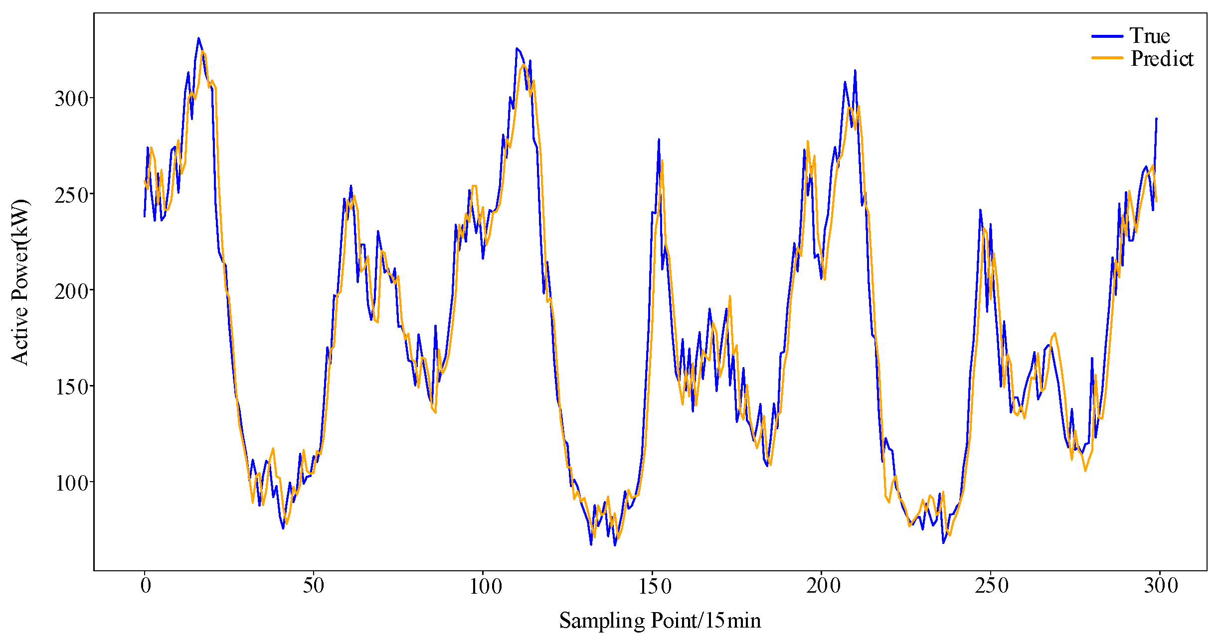
A time-series prediction model based on the Autoformer algorithm was established, and the prediction results are shown in Figure 4. Figure 4 illustrates a segment of the sequence without outliers, and it can be seen that the prediction results are relatively accurate. The comparison of this model with other time-series prediction models is shown in Table 6. From this table, it is evident that the time-series prediction model based on the Autoformer algorithm demonstrates the highest prediction accuracy. Compared to other algorithms, the RMSE, MSE, and MAE metrics are significantly reduced, while the R2 value increased to 0.922, indicating a better fit of the model to the data. The residual sequence can be used for outlier detection.

3.3.2. Detection Module

Outlier detection was performed on the residual sequence, and the detection results are shown in Table 7. In this study, precision, recall, and F1 score were selected as the evaluation metrics for the effectiveness of the outlier detection algorithm. The results show that the grid search-based RandomForest algorithm achieved the highest recall rate of 0.9974, indicating that it detected relatively more outliers. The F1 score was also the highest, reaching 0.9984, which represents a 15.4% improvement over the Decision Tree algorithm, a 6.7% improvement over the K-means algorithm, and a 1.1% improvement over the standard RandomForest algorithm. These results highlight the significant detection advantage of this approach, accurately identifying a greater number of outliers.

4. Conclusions

This study proposes a time-series anomaly detection model, AF-GS–RandomForest, for detecting anomalies in the time series of power consumption data. The main contributions of this work include the following: (1) the prediction component of the model, based on the Autoformer algorithm, effectively utilizes the sequence decomposition module, auto-correlation mechanism, and encoder–decoder modules to extract feature vectors from energy consumption data, enhancing the selection of critical information and fully leveraging historical data to predict energy consumption, thereby accurately reconstructing the residual sequence; and (2) an empirical analysis of the AF-GS–RandomForest algorithm was conducted, validating its effectiveness on typical datasets, and was successfully applied to a real dataset for detecting anomalies in energy consumption data.
This research primarily focuses on the detection of point anomalies. In future studies, methods for detecting and identifying anomalous time periods could be further explored. Additionally, as the methods chosen in this study rely heavily on high-accuracy prediction models, future research could focus on improving the structure of the prediction module to further enhance the algorithm’s prediction accuracy and robustness.
Author Contributions

Conceptualization, D.L. and Q.Y.; methodology, Z.M.; validation, B.Z.; validation, J.H.; data curation, D.L.; writing—original draft preparation, D.L.; writing—review and editing, D.L. All authors have read and agreed to the published version of the manuscript.

Funding

This research received no external funding.

Data Availability Statement

The original contributions presented in the study are included in the article, further inquiries can be directed to the corresponding author.

Conflicts of Interest

Authors Zhenghui Mao, Bijun Zhou, Jiaxuan Huang were employed by Longquan Power Supply Company, State Grid Zhejiang Electric Power Co., Ltd. The remaining authors declare that the research was conducted in the absence of any commercial or financial relationships that could be construed as a potential conflict of interest.

References

  1. Li, Z.; Zhang, Y. A New Hyperspectral Anomaly Detection Method Based on Higher Order Statistics and Adaptive Cosine Estimator. IEEE Geosci. Remote Sens. Lett. 2020, 17, 661–665. [Google Scholar] [CrossRef]
  2. Zou, T.; Gao, Y.; Yin, H.; Xu, C.; Xia, R.; Wu, C. Processing of Wind Power Abnormal Data Based on Thompson tau-quartile and Multi-point Interpolation. Autom. Electr. Power Syst. 2020, 44, 156–162. [Google Scholar]
  3. Yu, X.; Qi, L. Power Big Data Anomaly Detection Based on Stream Data Clustering Algorithm. Electr. Power Inf. Commun. Technol. 2020, 18, 8–14. [Google Scholar]
  4. Lee, H.; Kim, N.W.; Lee, J.G.; Lee, B.T. Performance-related Internal Clustering Validation Index for Clustering-based Anomaly Detection. In Proceedings of the 2021 International Conference on Information and Communication Technology Convergence (ICTC), Jeju Island, Republic of Korea, 20–22 October 2021; IEEE: Piscataway, NJ, USA, 2021; pp. 1036–1041. [Google Scholar]
  5. Yan, Y.; Qu, X.; Zhu, Q. Confidence measure method of classification results based on outlier detection. J. Nanjing Univ. Nat. Sci. 2019, 55, 8. [Google Scholar]
  6. Zheng, L.; Hu, W.; Min, Y. Raw wind data preprocessing: A data-mining approach. IEEE Trans. Sustain. Energy 2015, 6, 11–19. [Google Scholar] [CrossRef]
  7. Sun, Y.; Li, S.H.; Cui, C.; Li, B.; Chen, S.; Cui, G. Improved Outlier Detection Method of Power Consumer Data Based on Gaussian Kernel Function. Power Syst. Technol. 2018, 42, 1595–1604. [Google Scholar]
  8. Chou, J.S.; Tran, D.S. Forecasting energy consumption time series using machine learning techniques based on usage patterns of residential householders. Energy 2018, 165, 709–726. [Google Scholar] [CrossRef]
  9. Martin Nascimento, G.F.; Wurtz, F.; Kuo-Peng, P.; Delinchant, B.; Jhoe Batistela, N. Outlier Detection in Buildings’ Power Consumption Data Using Forecast Error. Energies 2021, 14, 8325. [Google Scholar] [CrossRef]
  10. Li, T.; Comer, M.L.; Delp, E.J.; Desai, S.R.; Mathieson, J.L.; Foster, R.H.; Chan, M.W. Anomaly Scoring for Prediction-Based Anomaly Detection in Time Series. In Proceedings of the 2020 IEEE Aerospace Conference, Big Sky, MT, USA, 7–14 March 2020; IEEE: Piscataway, NJ, USA, 2020; pp. 1–7. [Google Scholar]
  11. Li, C.; Liu, D.; Wang, M.; Wang, H.; Xu, S. Detection of Outliers in Time Series Power Data Based on Prediction Errors. Energies 2023, 16, 582. [Google Scholar] [CrossRef]
  12. Takahashi, K.; Ooka, R.; Kurosaki, A. Seasonal threshold to reduce false positives for prediction-based outlier detection in building energy data. J. Build. Eng. 2024, 84, 108539. [Google Scholar] [CrossRef]
  13. Solís-Villarreal, J.A.; Soto-Mendoza, V.; Navarro-Acosta, J.A.; Ruiz-y-Ruiz, E. Energy Consumption Outlier Detection with AI Models in Modern Cities: A Case Study from North-Eastern Mexico. Algorithms 2024, 17, 322. [Google Scholar] [CrossRef]
  14. Vaswani, A.; Shazzer, N.; Parmar, N.; Uszkoreit, J.; Jones, L.; Gomez, A.N.; Kaiser, Ł.; Polosukhin, I. Attention Is All You Need. In Proceedings of the 31st Conference on Neural Information Processing Systems (NIPS 2017), Long Beach, CA, USA, 4–9 December 2017; p. 5. [Google Scholar]
  15. Zhou, H.; Zhang, S.; Peng, J.; Zhang, S.; Li, J.; Xiong, H.; Zhang, W. Informer: Beyond efficient transformer for long sequence time-series forecasting. In Proceedings of the AAAI Conference on Artificial Intelligence, Virtual, 2–9 February 2021; Volume 35, pp. 11106–11115. [Google Scholar]
  16. Wu, H.; Xu, J.; Wang, J.; Long, M. Autoformer: Decomposition transformers with auto-correlation for long-term series forecasting. Adv. Neural Inf. Process. Syst. 2021, 34, 22419–22430. [Google Scholar]
  17. Tang, L.; Zhang, Z.; Chen, J.; Linna, X.U.; Zhong, J.; Yuan, P. Research on Autoformer-based electricity load forecasting and analysis. J. East China Norm. Univ. Nat. Sci. 2023, 5, 135–146. [Google Scholar]
  18. Zheng, H.; Xiao, F.; Sun, S.; Qin, Y. Brillouin Frequency Shift Extraction Based on AdaBoost Algorithm. Sensors 2022, 22, 3354–3365. [Google Scholar] [CrossRef] [PubMed]
  19. Yue, Y.; Li, K. Day-ahead prediction of V2G power capacity based on distribution Internet of Things technology and parallel random forest algorithm. Power Demand Side Manag. 2020, 22, 31–34. [Google Scholar]
Figure 1. Overall flow chart of the AF-GS–RandomForest model.
Energies 17 04810 g001
Figure 2. Autoformer Model Architecture Diagram.
Energies 17 04810 g002
Figure 3. Prediction Results based on the different algorithms for Electricity dataset.
Energies 17 04810 g003
Figure 4. Sequence prediction results based on the Autoformer algorithm.
Energies 17 04810 g004
Table 1. Comparison of the performance of the prediction algorithms on the ETT dataset.
ModelEvaluation Metrics
RMSEMSEMAER2
Transformer0.5430.5530.7370.511
Informer0.7380.6510.8590.334
Autoformer0.3880.4280.6230.65
Table 2. Comparison of the performance of the prediction algorithms on the Electricity dataset.
ModelEvaluation Metrics
RMSEMSEMAER2
Transformer0.3120.4030.5580.702
Informer0.2610.3660.5110.75
Autoformer0.2010.3150.4480.801
Table 3. Comparison of the performance of the prediction algorithms on the exchange rate dataset.
ModelEvaluation Metrics
RMSEMSEMAER2
Transformer0.3510.4580.5920.801
Informer0.6570.6430.810.627
Autoformer0.0640.1830.2530.964
Table 4. Comparison of predictive results on sequences that contain different proportions of outliers.
ModelOutliersEvaluation Metrics
MSEMAERMSER2
Autoformer3%_outlier0.2120.2430.4610.883
5%_outlier0.2040.2280.4520.888
10%_outlier0.2250.2550.4750.876
Informer3%_outlier0.630.5640.7930.654
5%_outlier0.6460.5770.8040.644
10%_outlier0.6560.5860.8120.639
Transformer3%_outlier0.4040.4370.6350.778
5%_outlier0.3930.4250.6270.784
10%_outlier0.4670.4750.6830.744
Table 5. Comparison of detection results on typical datasets.
ModelDateset NumberEvaluation Metrics
PrecisionRecallF1
GS–RandomForest10.97630.98120.9787
20.9990.9990.9999
30.95210.97050.9612
40.78240.78190.7822
RandomForest10.96380.97610.9691
20.9990.9990.9999
30.94570.96890.9411
40.76390.76480.7642
KNN10.9570.9490.9533
20.99980.99880.9993
30.93490.90060.9139
40.75590.76340.7596
Decision Tree10.92290.91350.9178
20.99980.99880.9993
30.85570.72660.7435
40.75910.76160.7603
Table 6. Performance Comparison of the Prediction Module.
ModelEvaluation Metrics
RMSEMSEMAER2
Autoformer21.064443.71216.0590.922
Informer24.806615.33919.2780.892
Transformer22.824520.96517.7730.907
Table 7. Outlier Detection Result Comparison of the Detection Module.
ModelEvaluation Metrics
PrecisionRecallF1
DecisionTree0.98780.73750.8445
K-means0.95620.90760.9313
RandomForest0.98850.98660.9875
GS–RandomForest0.99940.99740.9984
Disclaimer/Publisher’s Note: The statements, opinions and data contained in all publications are solely those of the individual author(s) and contributor(s) and not of MDPI and/or the editor(s). MDPI and/or the editor(s) disclaim responsibility for any injury to people or property resulting from any ideas, methods, instructions or products referred to in the content.