Article

Seismic Prediction Method of Shale Reservoir Brittleness Index Based on the BP Neural Network for Improving Shale Gas Extraction Efficiency

School of Petroleum and Natural Gas Engineering, Chongqing University of Science and Technology, Chongqing 401331, China
*
Author to whom correspondence should be addressed.
Energies 2024, 17(18), 4751; https://doi.org/10.3390/en17184751
Submission received: 30 July 2024 / Revised: 20 September 2024 / Accepted: 22 September 2024 / Published: 23 September 2024
(This article belongs to the Section H: Geo-Energy)

Abstract

:
The current seismic prediction methods of the shale brittleness index are all based on the pre-stack seismic inversion of elastic parameters, and the elastic parameters are transformed by Rickman and other simple linear mathematical relationship formulas. In order to address the low accuracy of the seismic prediction results for the brittleness index, this study proposes a method for predicting the brittleness index of shale reservoirs based on an error backpropagation neural network (BP neural network). The continuous static rock elastic parameters were calculated by fitting the triaxial test data with well logging data, and the static elastic parameters with good correlation with the brittleness index of shale minerals were selected as the sample data of the BP neural network model. A dataset of 1970 data points, characterized by Young’s modulus, Poisson’s ratio, shear modulus, and the mineral brittleness index, was constructed. A total of 367 sets of data points from well Z4 were randomly retained as model validation data, and 1603 sets of data points from the other three wells were divided into model training data and test data at a ratio of 7:3. The calculation accuracy of the model with different numbers of nodes was analyzed and the key parameters of the BP neural network structure such as the number of input layers, the number of output layers, the number of hidden layers, and the number of neurons were determined. The gradient descent method was used to determine the weight and bias of the model parameters with the smallest error, the BP neural network model was trained, and the stability of the brittleness index prediction model of the BP neural network was verified by posterior data. After obtaining Young’s modulus, Poisson’s ratio, and shear modulus through pre-stack seismic inversion, the BP neural network model established in this study was used to predict the brittleness index distribution of the target layer in the study area. Compared with the conventional Rickman method, the prediction coincidence rate is 69.16%, and the prediction coincidence rate between the prediction results and the real value is 95.79%, which is 26.63% higher. The BP neural network method proposed in this paper provides a reliable new method for seismic prediction of the shale reservoir brittleness index, which has important practical significance for clarifying the shale gas development scheme and improving shale gas exploitation efficiency.

1. Introduction

Shale gas refers to the free or adsorption state occurrence of unconventional gas in the organic matter of shale and source rocks [1]. Due to the characteristics of the low porosity and low permeability of shale reservoirs, the effective exploitation of shale gas depends on the volumetric fracturing of reservoirs, and the brittleness index is the main factor affecting the quality of reservoir fracturing [2]. Therefore, the prediction of the brittleness index of a shale reservoir is very important in shale gas exploitation.
The characterization of the brittleness index was divided into two quantitative indicators: the mineral brittleness index based on rock mineral composition, and the elastic parameter brittleness index based on Young’s modulus, Poisson’s ratio, and other elastic parameters [3]. Jarvie et al. [4] analyzed the mineral composition of Barnett shale and identified quartz as the primary brittleness mineral, and suggested that the proportion of quartz in the rock composition reflects brittleness. Wang et al. [5] pointed out that, in addition to quartz, dolomite is a significant brittle mineral component. Furthermore, Li et al. [6] suggested that in shale reservoirs with high carbonate mineral content, the influence of carbonate minerals on brittleness should be fully considered. Building on previous research, Jin et al. [7] further clarified that quartz, feldspar, mica, and carbonate minerals are brittle mineral components. Obviously, the key to characterizing the brittleness index based on rock brittle mineral components lies in defining brittle minerals. Rickman et al. [8], based on their experience with Barnett shale exploration and development, analyzed that shale with a high Young’s modulus and low Poisson’s ratio has stronger brittleness. They first proposed to comprehensively characterize shale brittleness using Young’s modulus and Poisson’s ratio. Goodway et al. [9] proposed using Lame parameters and shear modulus to characterize shale brittleness. Guo et al. [10] and Liu et al. [11] further pointed out the use of the quotient of Young’s modulus and Poisson’s ratio to characterize brittleness. Therefore, the characterization of the brittleness index based on Young’s modulus and Poisson’s ratio is not singularly related to these two elastic parameters, and should also consider other elastic parameters such as Lame parameters and shear modulus.
The prediction of the brittleness index could be categorized into two main types: two-dimensional well logging prediction and three-dimensional seismic prediction. Methods for well logging prediction currently include conventional elastic wave logging, full-waveform elastic wave logging, arrayed elastic wave logging, dipole elastic wave logging, and elemental capture logging. These methods calculate the longitudinal single-well distribution of the brittleness index [12]. However, predicting the brittleness index solely using logging methods may not meet practical demands. Therefore, seismic prediction of the brittleness index has become a significant research focus in shale gas exploration.
At present, there are few methods to directly obtain the brittleness index from 3D seismic exploration data. The commonly used reservoir brittleness index prediction method in actual production was the seismic prediction method based on pre-stack data [13]. This method utilized the method of the simultaneous inversion of pre-stack earthquakes, by applying multiple pre-stack earthquake data volumes for simultaneous inversion, to obtain elastic parameter data volumes, such as Young’s modulus and Poisson’s ratio. Then, by calculating the elastic parameter data volume through linear mathematical relationships or using nonlinear multiple regression models, the brittleness index data volume could be directly or indirectly obtained, and the three-dimensional transverse and longitudinal brittleness index distribution of shale gas reservoirs could be obtained. Wang Lei [14] comprehensively analyzed the mineral composition and logging interpretation data of multiple wells in the Jiaoshiba area, and predicted the brittle distribution law of the area by simultaneously inverting the ratio of the elastic parameters Young’s modulus and Poisson’s ratio before stacking. Wang et al. [15] established a new shale brittleness assessment method based on elastic parameters such as compressional wave and shear wave impedance, Lame coefficient, Poisson’s ratio, and Young’s modulus. They predicted the brittleness index distribution of shale gas reservoirs in the region by simultaneously inverting the brittleness index data volume before stacking. Zhang et al. [16] proposed to establish a multivariate nonlinear regression brittle index prediction model and use the pre-stack seismic inversion method to obtain the required elastic parameters for three-dimensional seismic data to achieve the brittle index prediction of shale layers in the study area. Shan et al. [17] combined the pre-stack inversion results to calculate the compressional wave and shear wave velocities, shear wave impedance, Lame coefficient, and shear impedance data volumes. Then, using the multiple regression relationship between the brittleness index and the calculated elastic parameter data volume, they predicted the brittleness index in the Nanchuan area. However, in the above methods, the mathematical relationship conversion formula between the elastic parameters and brittleness index is only based on simple linear mathematical relationships for a few elastic parameters, and the multiple regression model is easily affected by factors such as model parameter selection and error verification. The accuracy of brittleness index prediction results needs to be further improved.
The BP neural network exhibited strong fitting and predictive capabilities for nonlinear data, along with model optimization ability, and has gradually been applied in the petroleum and natural gas exploration and development industry [18]. Wu et al. [19] first employed the BP neural network to establish a network model between oil and gas reservoirs and the extracted seismic channel characteristic parameters, achieving lateral prediction of oil and gas reservoirs in the study area. Zhu et al. [20] utilized the BP neural network to establish a nonlinear correlation model, reflecting multiple parameters of seismic data with the lateral variation of reservoirs. They applied the model to the entire study area to achieve the plane distribution of sand thickness and mud content in the Dalinhe oil layer. Wang et al. [21] integrated geological, well logging, drilling, and core analysis data to establish a BP neural network prediction model. They used core data and logging data as inputs, porosity, and permeability identification parameters as output targets, determining the distribution of reservoir porosity and permeability in the study area. Okon et al. [22] proposed using the BP neural network method to train gamma-ray logging resistivity logs, such as density, and interval logs, to predict the reservoir rock physical properties of porosity, permeability, and water saturation. Saikia et al. [23] further emphasized that applying the BP neural network can assist in determining reservoir characteristics by analyzing the correlation of geological and geophysical data. However, researchers currently have found that the BP neural network is primarily used to predict reservoir parameters, with limited research and application in the field of seismic nonlinear prediction of the brittleness index.
Therefore, this study proposed to address the shortcomings of conventional seismic prediction methods for the brittleness index, and the issue of low prediction accuracy. This study introduced the BP neural network into seismic prediction research of the brittleness index, and proposed a BP neural network-based method, for predicting the brittleness index, through seismic data. Based on the BP neural network algorithm, this study aimed to construct a brittleness index prediction model, and performed model optimization to fully explore and obtain the nonlinear relationship between the brittleness index and the different elastic parameters. The effectiveness of the method was validated by analyzing prediction errors. This model was applied across the entire study area to predict the brittleness index, and it enhanced the accuracy of seismic prediction of the brittleness index in this area, and enabled more precise identification of favorable fracturing zones within shale reservoirs. The BP neural network prediction method proposed in this study provided a new idea for the seismic prediction of the brittleness index in shale formations.

2. Principles

This study was based on the prediction results of rock elastic parameters such as Young’s modulus, Poisson’s ratio, and shear modulus by seismic pre-stack simultaneous inversion. The network model for predicting rock brittleness based on rock elastic parameters established by the BP neural network algorithm was used to realize the prediction method of the shale reservoir brittleness index, which mainly involves two core theories: pre-stack simultaneous inversion and the BP neural network.

2.1. Principle of Predicting Rock Elastic Parameters through Pre-Stack Simultaneous Inversion

The theoretical basis for pre-stack simultaneous inversion comprised the Zoeppritz equation and the Fatti simplified expression, as illustrated in Equations (1) and (2). This inversion technique utilized pre-stack gather data, well logging curves, and seismic layer data for inversion, thereby obtaining compressional wave data, shear wave data, and density data volumes. The methodology involved the following steps: the optimization and processing of seismic data, standardization of logging curves, extraction of seismic wavelets, and generation of synthetic seismic records; the establishment of a low-frequency model by integrating seismic interpretation layers with logging curves as constraints; and using seismic data volumes, well logging curves, and stratigraphic layers as data inputs to obtain the final inversion data volumes.
sin θ 1 cos φ 1 sin θ 2 cos φ 2 cos θ 1 sin φ 1 cos θ 2 sin φ 2 sin 2 θ 1 V p 1 V s 1 cos 2 φ 1 ρ 2 V s 2 2 V p 1 ρ 1 V s 1 2 V p 2 sin 2 θ 2 ρ 2 V s 2 V p 1 ρ 1 V s 1 2 cos 2 φ 2 cos φ 1 V s 1 V p 1 sin θ 1 ρ 2 V p 2 ρ 1 V p 1 cos 2 φ 2 ρ 2 V s 2 ρ 1 V p 1 sin φ 2 R p p R p s T p p T p s = sin θ 1 cos θ 1 sin 2 θ 1 cos 2 φ 1 ,
In Equation (1), R p p is the compressional wave reflection coefficient, R p s is the converted shear wave reflection coefficient, T p p is the compressional wave transmission coefficient, T p s is the converted shear wave transmission coefficient, V p 1 , V p 2 are the compressional wave velocities of the rock at the upper and lower interfaces, respectively, V s 1 , V s 2 are the shear wave velocities of the rock at the upper and lower interfaces, respectively, and ρ 1 , ρ 2 are the densities of the rock at the upper and lower interfaces, respectively.
R p p θ = C 1 R p + C 2 R s + C 3 R D ,
In Equation (2), R p = 1 2 Δ V p V p + Δ ρ ρ ,   R s = 1 2 Δ V s V s + Δ ρ ρ ,   R D = Δ ρ ρ , Δ ρ ρ = 1 4 Δ V p V p ,   C 1 = 1 + tan 2 θ ,   C 2 = 8 Υ 2 sin 2 θ ,   C 3 = 2 Υ 2 sin 2 θ 1 / 2 tan 2 θ .

2.2. Principle of BP Neural Network

The BP neural network was proposed by Rumelhart et al. in 1986 and remains one of the most widely used neural network models [24]. It imitates the structure of human neural networks by constructing a mathematical model composed of multiple neurons, to realize functions such as numerical prediction, pattern recognition, curve fitting, and feature extraction [25]. The BP neural network model structure consists of an input layer, an output layer, and any number of hidden layers, each consisting of several neurons [26]. As illustrated in Figure 1, the BP structure exhibited three key characteristics: each neuron receives input from every neuron in the preceding layer; its output was transmitted to each neuron in the subsequent layer; and neurons within the same layer lack interconnections. During training, the model adhered to the principle of minimizing the error between desired and actual outputs, and continuously updated the weights (w) and thresholds (b) of neurons in the hidden and input layers, through backpropagation of errors from the output layer. The BP neural network determined the number of neurons in the output and input layers by analyzing the input feature variables that affect the target variable. The number of neurons in the hidden layers was determined through trial and error, thus defining the network model structure. The network model was subsequently trained and evaluated to minimize model error. Validation data were used to verify the network model, and upon satisfactory validation results, the BP neural network construction was deemed complete.

3. Materials and Methods

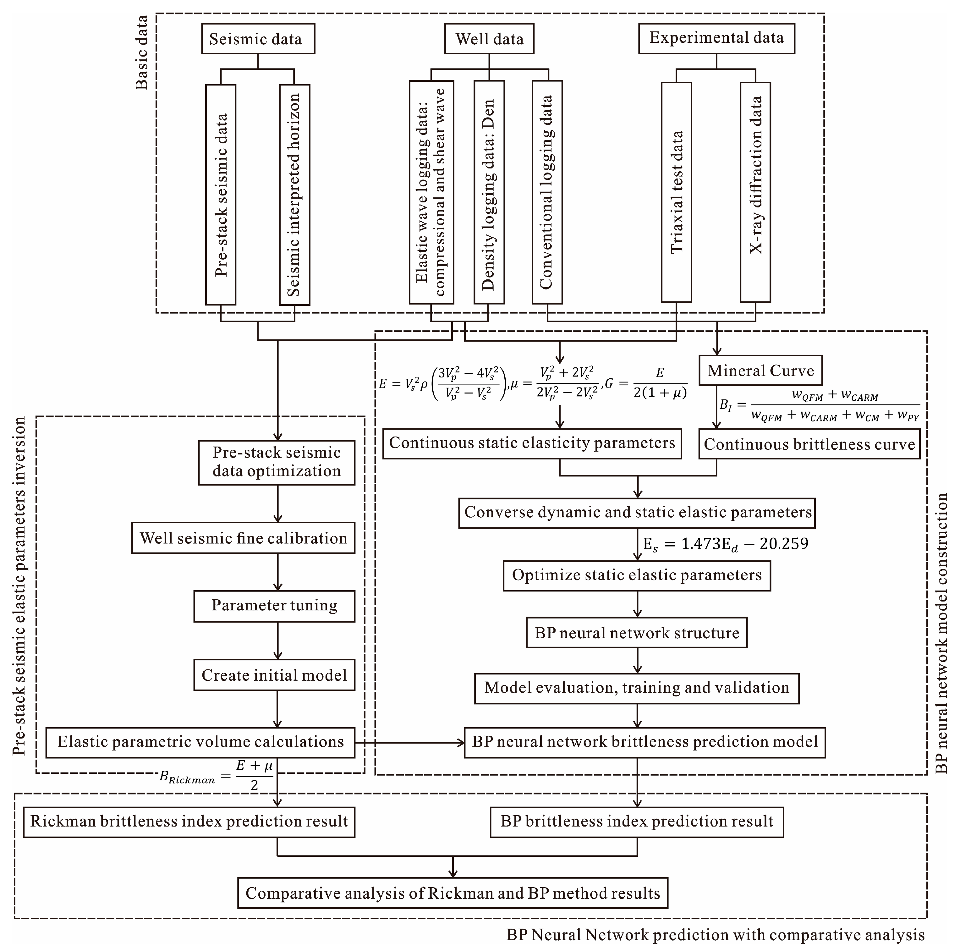
Figure 2 shows the study flowchart of the seismic prediction method of the shale reservoir brittleness index, based on the BP neural network. The research process included three main steps: BP neural network model construction, pre-stack seismic elastic parameters inversion, and BP neural network prediction with comparative analysis.

3.1. BP Neural Network Construction

3.1.1. Data Preprocessing

  • Rock elastic parameter data
The continuous dynamic rock elastic parameter data needed to be unified and corrected to static parameters. Static parameters were obtained through indoor rock mechanics experiments, such as the triaxial test, to obtain rock parameters like Young’s modulus and Poisson’s ratio. Dynamic parameters were rock elastic parameters calculated using array elastic wave logging data [27]. The static parameters of rocks had the advantages of high accuracy and reliable data, but the limited number of experimental data points could not meet the requirements for training data for neural networks.
Therefore, a large number of uniform data points for static elastic parameters could be obtained by correcting the continuous dynamic elastic parameters. The dynamic and static Young’s moduli of rocks exhibited a linear relationship, but the relationship between dynamic and static Poisson’s ratios remained unclear [28]. Static elastic parameter data of shale reservoirs in the Longmaxi Formation submember of the Yuxi Z Block, Sichuan Basin, were obtained through the triaxial test. Dynamic elastic parameter data were calculated from cross-dipole sonic logging data. By fitting the dynamic and static elastic parameters, a formula was derived to convert dynamic to static rock parameters, achieving static calibration of dynamic parameters and providing sufficient data points for training neural network models.
To eliminate the interference of different dimensional units between elastic parameters, Equation (3) was used to normalize the elastic parameters. After processing, the dimensions were unified and the correlation remained unchanged.
Z i = X i m i n X i m a x X i m i n X i ,
In Equation (3), Z i represents the normalized value of each elastic parameter, X i represents the original value of each elastic parameter, and m a x X i , m i n X i are the maximum and minimum values of each elastic parameter.
2.
Brittleness index data
Using conventional logging data and X-ray diffraction mineral composition data, a logging interpretation template was established to derive continuous mineral curves. Equation (4) was applied to calculate these mineral curves, and obtain continuous data points for the mineral brittleness index.
B I = w Q F M + w C A R M w Q F M + w C A R M + w C M + w P Y ,
In Equation (4), B I represents the mineral brittleness index; w Q F M is the quartz and feldspar content in shale, %; w C A R M is the calcite and dolomite content in shale, %; w C M is the clay mineral content in shale, %; and w P Y is the pyrite content in shale, %.
3.
Sensitivity analysis of elastic parameters
The mineral brittleness index and normalized elastic parameters were crossed and analyzed, and the elastic parameters with good correlation were selected as the sensitive elastic parameters for predicting the brittleness index. The larger the absolute value of the correlation coefficient, closer to 1 or −1, the stronger the correlation; closer to 0 indicated a weaker correlation.

3.1.2. BP Neural Network Model Structure

For any continuous function in a closed interval, an arbitrary n-dimensional to m-dimensional mapping could be accomplished by a three-layer BP neural network with a single hidden layer structure [29]. In this study, a three-layer BP neural network was used with a single input layer, a single output layer, and a single hidden layer. The number of neurons in the input layer of the BP neural network was determined by the number of selected sensitive elastic parameters. The number of neurons in the output layer was determined by the number of prediction objectives. The number of nodes in the hidden layer of the model was determined through the trial-and-error method, with the specific number of nodes being set while keeping other parameters constant. The optimal number of neurons in the hidden layer was determined by analyzing and comparing the computational accuracy at different numbers of increasing nodes.

3.1.3. Model Training and Evaluation Criteria

This study was based on the first Submember of Longmaxi Formation shale reservoir in the Z block of Sichuan Basin. The target interval was divided into four small layers from top to bottom, namely, the first Submember of layer 4, layer 3, layer 2, and layer 1. The lithology was characterized by gray-green mudstone interbedded with gray shale in the upper and middle parts, and deep gray, gray-black, and black shale in the lower part, with the color becoming darker from top to bottom. Preprocessing the actual logging data, rock mechanics experimental data and X-ray diffraction experimental mineral data of the target interval, the continuous mineral brittleness index data, and the corresponding elastic parameter data of each brittleness index sensitive rock were obtained. Eliminating outliers, the dataset that can be used for model training and validation was determined. Continuous data of 3 wells were randomly selected to participate in model training.
To evaluate the predictive performance of the model, the Mean Absolute Error (MAE) and coefficient of determination (R2) were selected as the model performance evaluation metrics. The MAE assessed the difference between predicted and actual values, expressed as an absolute value. Lower MAE values indicated higher model accuracy. R2 evaluated the correlation between predicted and actual values; values closer to 1 indicated a stronger correlation and higher model reliability. The equations for calculating MAE and R2 are provided below.
M A E = 100 1 n i = 1 n y ^ i y i y i ,
R 2 = i = 1 n y ^ i y ^ ¯ y i y ¯ 2 i = 1 n y ^ i y ^ ¯ 2 i = 1 n y i y ¯ 2 ,
In the equations above, n represents the number of samples, y ^ i represents the predicted value of the ith sample, y i   represents the true value of the ith sample, y ^ ¯   represents the mean of predicted values for the samples, and y ¯ denotes the mean of true values for the samples.

3.1.4. Effectiveness Verification

Model validation data were selected from the single well that was not included in the model training process to analyze and validate the effectiveness of the BP neural network brittleness index prediction model. The coefficient of determination (R2) was used to assess the model’s predictive performance by analyzing the correlation between predicted and actual values from this well.

3.2. Pre-Stack Seismic Elastic Parameters Inversion

3.2.1. Pre-Stack Seismic Data Optimization and Well Seismic Fine Calibration

The seismic data were processed by super-gather techniques to obtain high signal-to-noise ratio seismic data. The processed seismic data were further converted into pre-stack angle gathers, which maximally retain the information of seismic amplitude variation with offset, providing reliable seismic data for pre-stack inversion.
Strong seismic reflection interfaces, extracted seismic wavelets, and well logs were used for calibration to establish an accurate correspondence between well logs and seismic data, and to clarify the reservoir’s response characteristics in the seismic data. The principle of seismic wavelet extraction aimed to maximize the correlation coefficient between synthetic records and seismic traces, further optimizing seismic wavelet parameters for accurate extraction.

3.2.2. Elastic Parametric Data Volumes’ Calculation

Initial models of the compressional wave velocity, shear wave velocity, and density necessary for inversion were established, based on well location information, horizon information, and seismic wavelets. Actual seismic data were used to conduct pre-stack inversion and obtain the inverted data volumes of compressional wave velocity, shear wave velocity, and density. Further, rock mechanics formulas were applied to derive data volumes of optimal sensitive elastic parameters.

3.3. Seismic Prediction of Brittleness Index in Shale Reservoirs Based on BP Neural Network

The reservoir brittleness index sensitive elastic parameter data volume obtained by seismic data inversion was used as the input data for the neural network. The trained and validated neural network system was used to predict the shale reservoir brittleness index data volume, and then the seismic prediction results of the brittleness index in the study area based on the BP neural network were obtained.

4. Results

4.1. BP Neural Network Model Construction

4.1.1. Data Preprocessing Results

  • Static and normalization correction of rock mechanical parameters
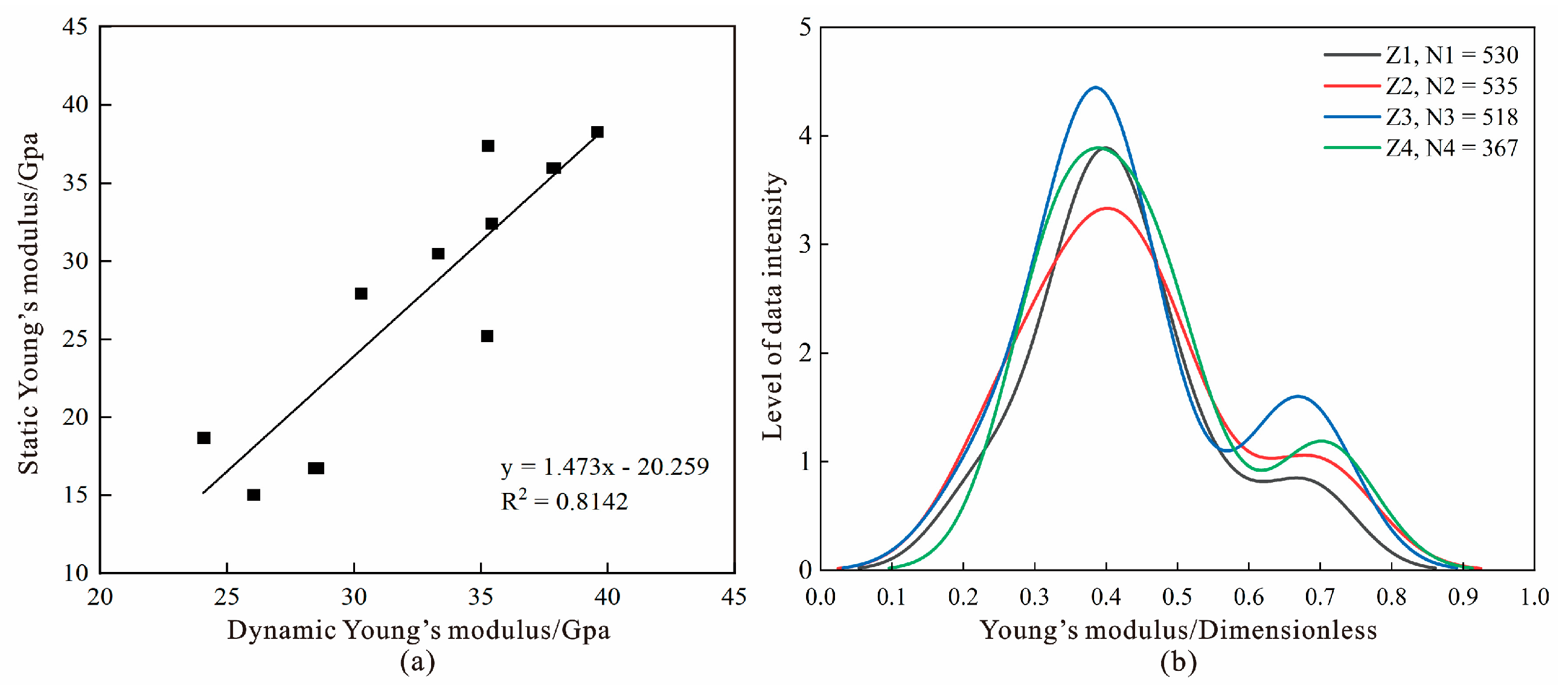
The static Young’s modulus obtained from 10 sets of laboratories in the study area was used to fit the dynamic parameter data at the corresponding depth points (Figure 3a). The coefficient of determination for the regression plot reached 0.8142, indicating a good fit. The equation for the static Young’s modulus correction was derived as follows:
E s = 1.473 E d 20.259 ,
In Equation (7), E s is the static Young’s modulus, MPa; E d is the dynamic Young’s modulus, MPa.
In this study, data points from four wells, Z1, Z2, Z3, and Z4, which could simultaneously have rock mechanics parameters and brittleness index data in the research area, were used as the basic data for constructing a neural network. Static correction formulas were used to correct continuous dynamic rock mechanical parameters, and a total of 1970 dynamic rock mechanics data points from four wells were corrected (Figure 3b).
Figure 3. Dynamic and static Young’s modulus fitting and data normalization: (a) fitting analysis plot; (b) plot of normalized results.
Energies 17 04751 g003
2.
Brittleness index data
Brittleness index curve data for four target layers from the mineral method were obtained, with a total of 1970 consecutive brittle index data points, as shown in Figure 4. Figure 5 shows the X-ray diffraction data, compressional and shear wave curves, and elastic parameter data for well Z1.
3.
Optimization results of sensitive rock mechanics parameters
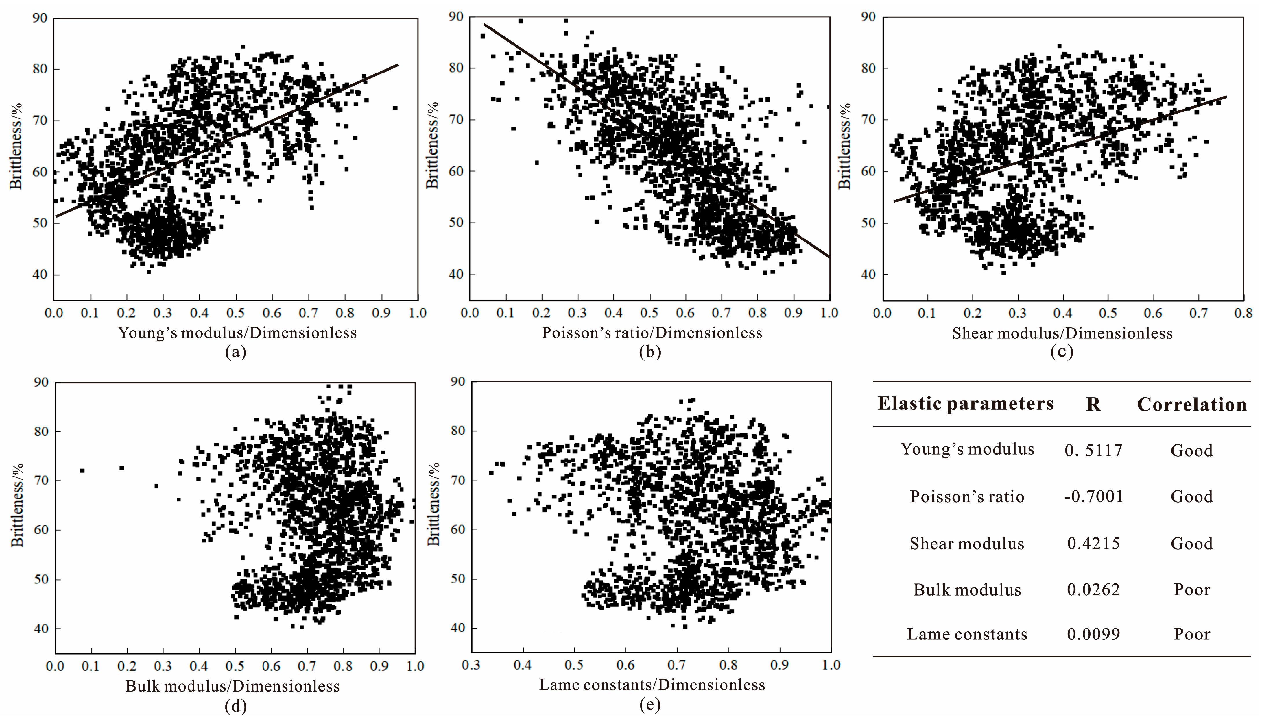
The intersection analysis of various rock mechanics parameters and the shale brittleness index has revealed that the brittleness index exhibited a relatively good correlation with Young’s modulus, Poisson’s ratio, and shear modulus, but showed a poor correlation with bulk modulus and Lame constants (Figure 6). Thus, Young’s modulus, Poisson’s ratio, and shear modulus were chosen as the three sensitive elastic parameters for input into the predictive model of the shale brittleness index.

4.1.2. Determination of Network Structure

Based on the selected sensitive elastic parameters results, Young’s modulus, Poisson’s ratio, and shear modulus were constructed as input layers for the model. The brittleness index served as the output layer. Thus, the input layer of the network was specified as three neurons, and the output layer was specified as one neuron.
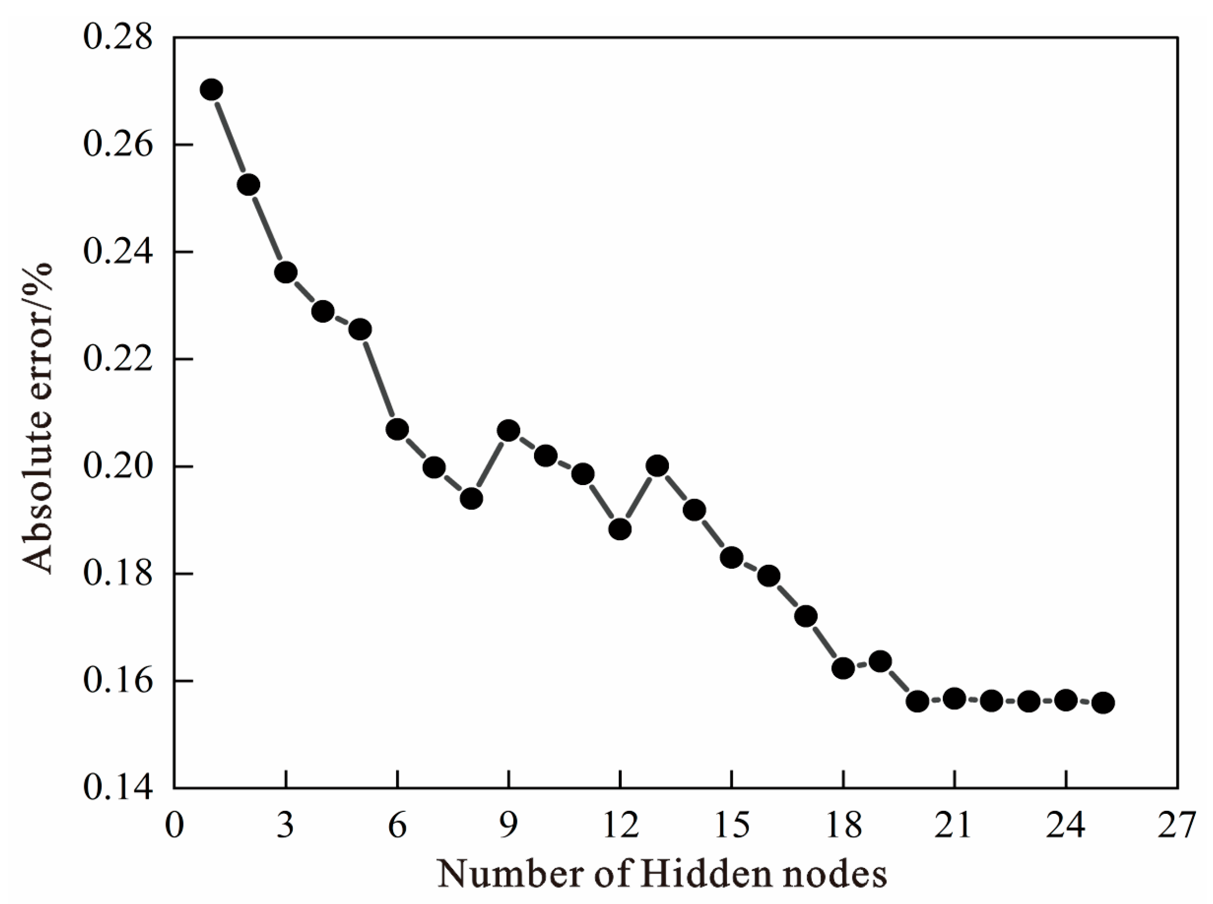
The trial-and-error method was employed to determine the number of neurons in the hidden layer. Analysis of the total error corresponding to different numbers of hidden layer nodes, with 20 nodes in the hidden layer, showed the absolute error reached 0.15616 (as shown in Table 1 and Figure 7). The absolute error tended to stabilize as the number of nodes continued to increase. Thus, the number of neurons in the hidden layer was selected to be 20.
In summary, the BP neural network model in this study configured a three-layer structure, consisting of a single input layer, a single hidden layer, and a single output layer. The input layer consisted of 3 neurons, the hidden layer consisted of 20 neurons, and the output layer consisted of 1 neuron.

4.1.3. Model Training and Testing

The data from the Young’s modulus (E), Poisson’s ratio (μ), and shear modulus (G) from four wells, Z1, Z2, Z3, and Z4, with cross-dipole elastic wave logging data and rock and mineral logging interpretation data in the study area, were used as input feature variables for the model. The corresponding brittleness index data served as the output feature variable. The four wells provided a total of 1970 sets of valid data points. Well Z4 was randomly retained as posterior data, while the remaining 1603 sets of data points from wells Z1, Z2, and Z3 were utilized for the training and testing of the network system. According to the widely used dataset partitioning method, the 1603 sets of data points were divided into training data (70%) and test data (30%). An absolute error analysis, which showed that the relative error of the BP neural network prediction model was relatively small with an average of 3.10%, was conducted between the predicted value of the system and the actual brittleness index. Table 2 presents part of the training data and error analysis data. The correlation analysis between the predicted results of the system training data and the actual brittleness data showed that the correlation coefficient between the two was 0.9346 (Figure 8a). The correlation analysis between the predicted results of the system test data and the actual data showed that the correlation coefficient between the two was 0.9214 (Figure 8b). The model training and testing results were good.

4.1.4. Model Effect Verification

Three rock elastic parameters in 367 groups of data points of well Z4 that were not involved in model training and system testing were used as input, and the brittleness index output by the neural network was compared and analyzed with the corresponding actual brittleness index. As can be seen from Figure 9, the brittleness index of five core samples based on triaxial test data is similar to the real brittleness index of minerals and the predicted brittleness index data of the BP method, indicating that the real and predicted values of the brittleness index can be used to verify and evaluate the prediction results of the brittleness index. The predicted value of the longitudinal brittleness index of well Z4 in the study area obtained by using the BP neural network model has a high matching degree with the real value, and the correlation coefficient of prediction of 367 data points of well Z4 is 0.811. The neural network model established in this study has a good consistency.

4.2. Elastic Parameter Inversion Volumes Calculation

High-quality pre-stack seismic data were obtained by applying super-gather processing techniques to the original CDP gathers (Figure 10a). The Super CDP gathers (Figure 10b) were then converted into AVA gather data for pre-stack simultaneous inversion (Figure 10c). In the comparison of the original CDP gathers in Figure 9 with the optimized Super CDP gathers, gather quality was significantly improved, and the signal-to-noise ratio was significantly increased. The target layer in the synthetic seismic record from a single well showed strong amplitude peak reflection (Figure 10d).
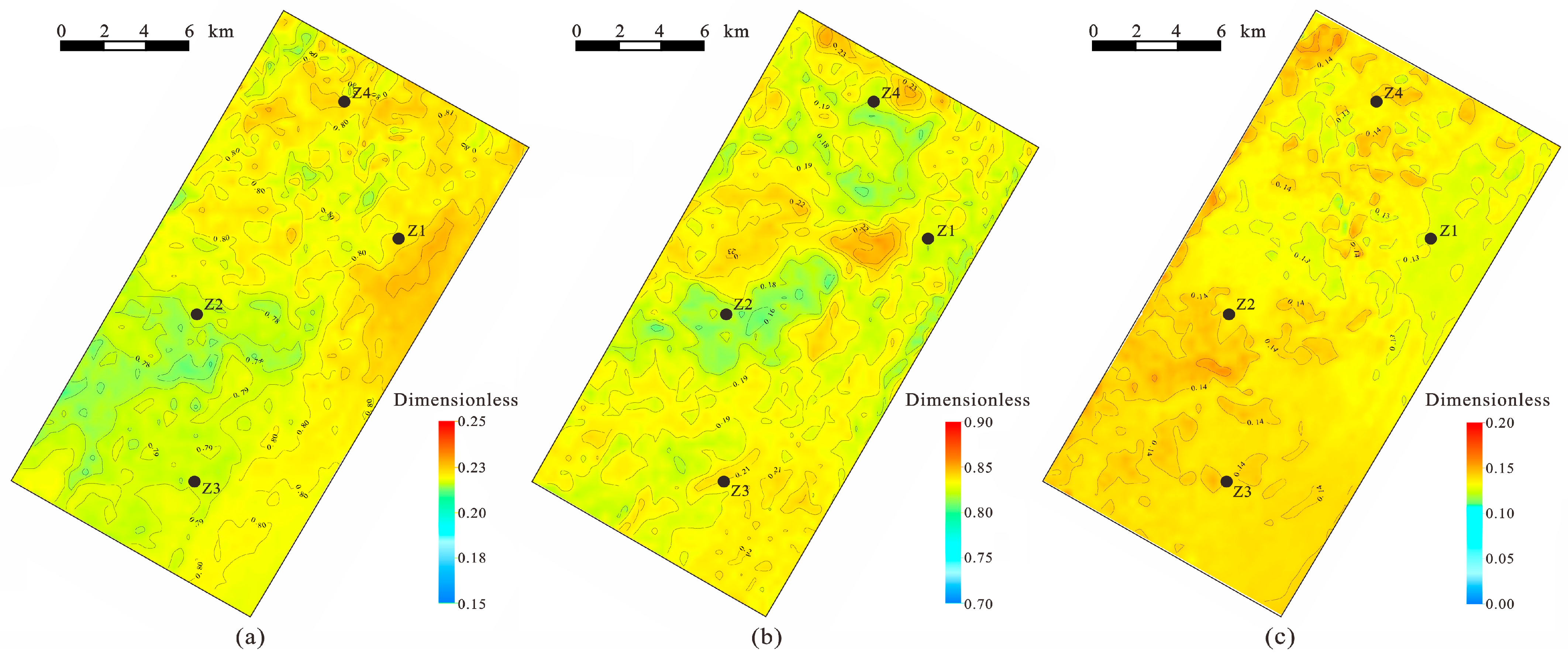
Under the constraints of horizon data, well data, and geological models, the compressional wave velocity, shear wave velocity, and density data volumes were jointly inverted to derive the data volumes of the Young’s modulus, Poisson’s ratio, and shear modulus elastic parameters. Figure 11 displays the plane diagrams of these elastic parameter data volumes. Young’s modulus exhibits a distribution pattern from low in the southwest to high in the northeast, while Poisson’s ratio and shear modulus show a higher-to-lower distribution from southwest to northeast. Young’s modulus and Poisson’s ratio exhibit a negative correlation, consistent with the results of the shale brittleness index cross-plot analysis.

4.3. Brittleness Index Seismic Prediction

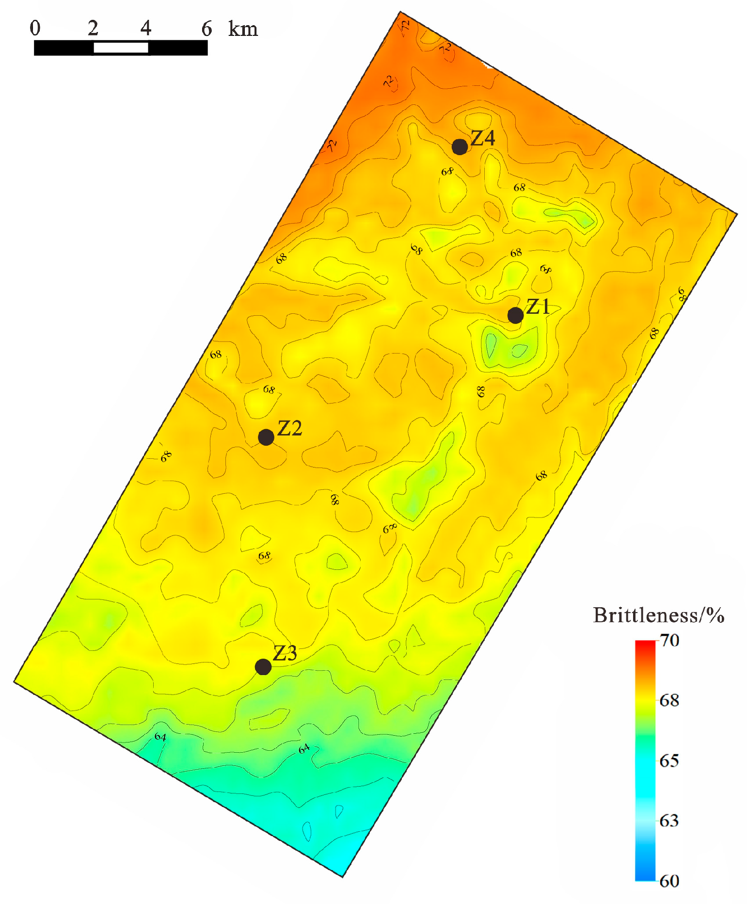
The predicted data volumes of Young’s modulus, Poisson’s ratio, and shear modulus from the pre-stack inversion were inputted into the constructed neural network model to obtain the brittleness index prediction results. Figure 12 shows the distribution of these predicted results. Analysis of the BP neural network’s prediction of the brittleness index showed the average brittleness index was between 60% and 70%, and the brittleness index gradually decreased in a northwest-to-southeast pattern.

5. Discussion

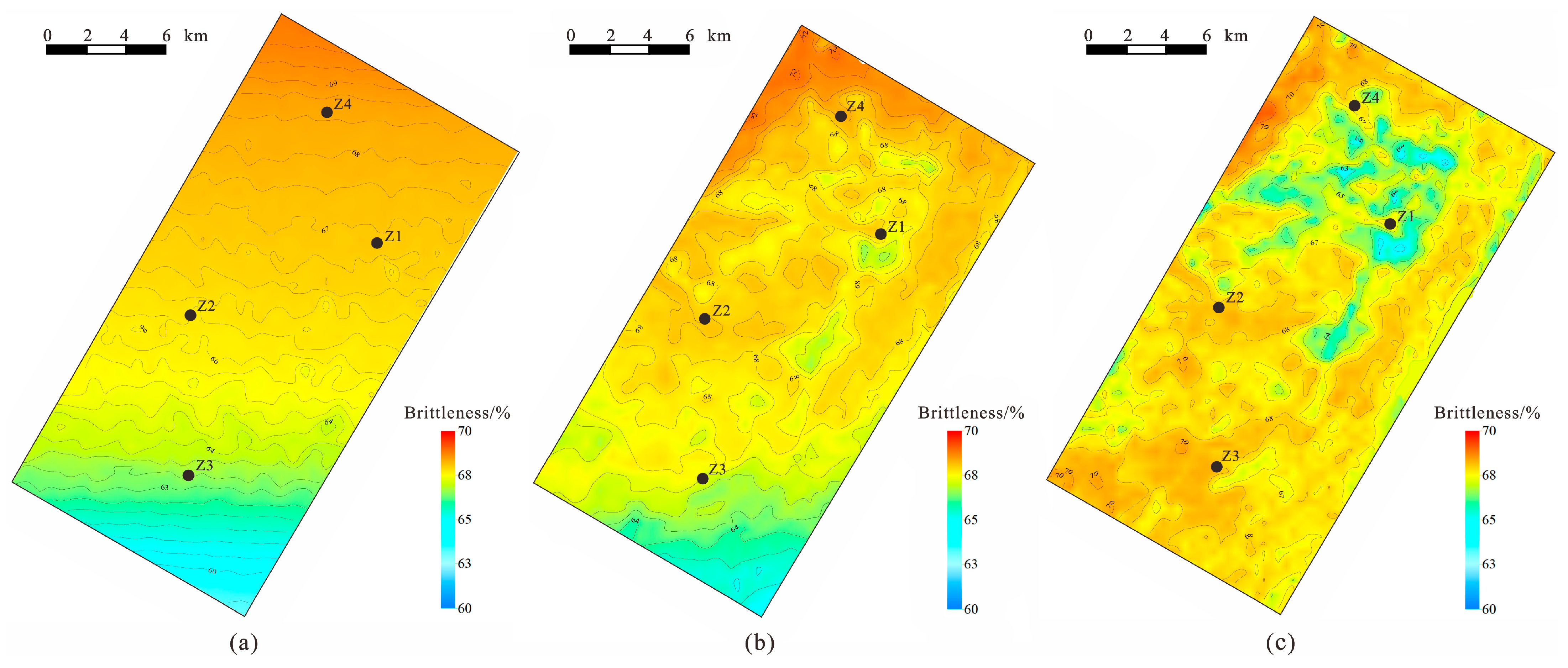
To recognize the differences between the BP method and the traditional method, the predicted brittleness index results of the conventional Rickman method were compared with the BP neural network method. The analysis of the two methods for predicting the brittleness index and the interpolation of the wellbore brittleness data plane showed that the actual mineral brittleness index plane diagram (Figure 13a) was consistent with the BP neural network method brittleness index prediction results (Figure 13b). The average brittleness index of the wells was between 60% and 70%, and the brittleness index plane diagram showed a trend of decreasing from northwest to southeast. The predicted plane diagram of the conventional Rickman method’s brittleness index (Figure 13c) has gaps compared with the actual well-point brittleness index data plane diagram.
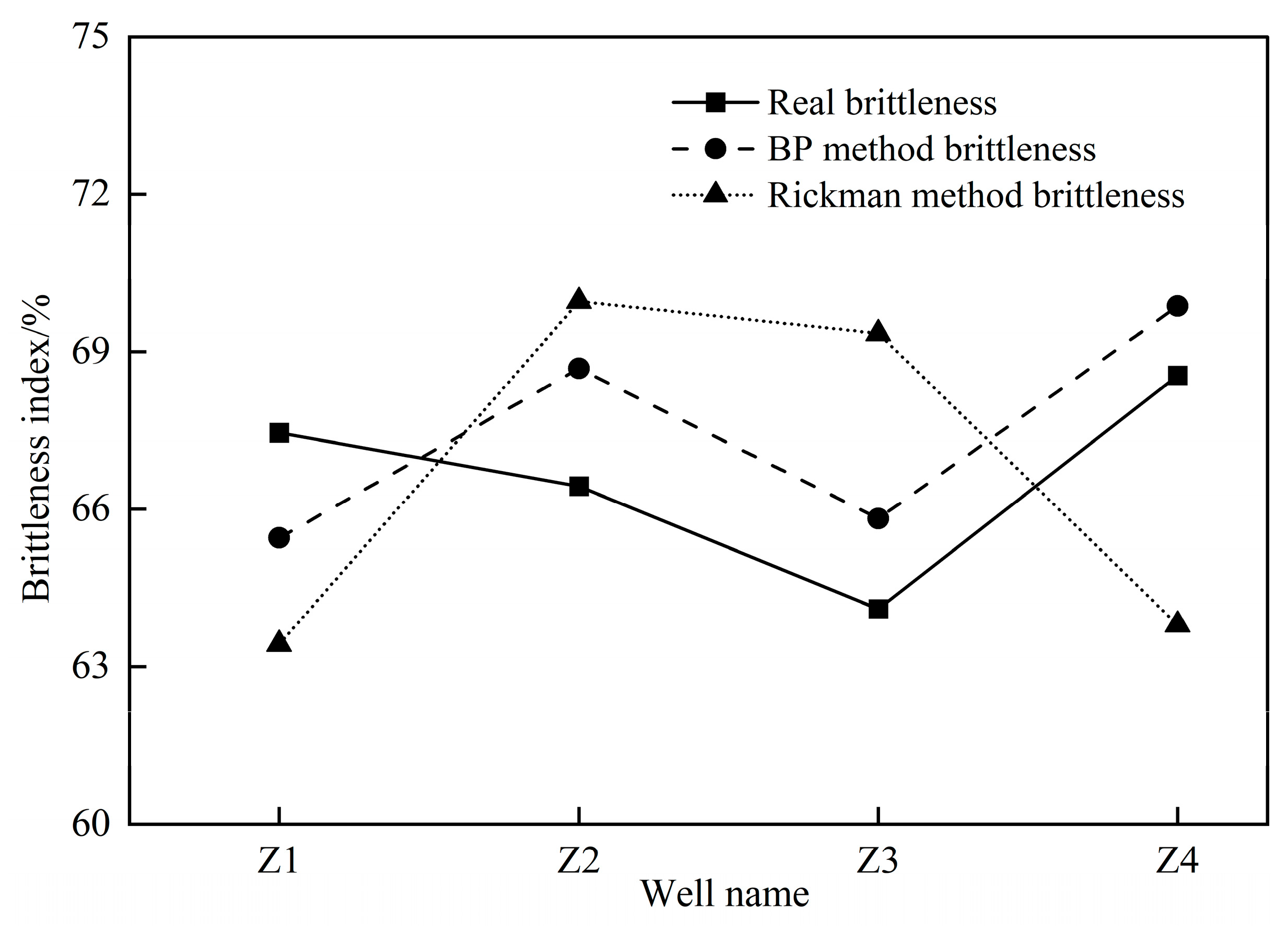
The comparison between the predicted value and the actual value of the average brittleness index of the target layer of a single well and the statistical analysis of the error (Table 3 and Figure 14) showed that the maximum relative error of the average brittleness index of the target layer of the well point predicted by this method was 2.74%, while the maximum relative error of the average brittleness index of the Rickman brittleness index prediction method was 6.60%.
The relative error between the predicted value and the actual value of the 1970 group of data points was counted, and the prediction effect of the two methods was compared and analyzed (Figure 15). If the relative error was <±5%, the prediction was defined as consistent, otherwise it was not consistent [30], and then, the coincidence rate of the brittleness index earthquake prediction results of the BP neural network method was 95.79%. The coincidence rate of Rickman’s seismic prediction results was 69.16%. The prediction coincidence rate of the proposed method based on the BP neural network was 26.63% higher than the traditional method.

6. Conclusions

  • In this study, the BP neural network was used for the seismic prediction of the shale brittleness index. Three elastic parameters (Young’s modulus, Poisson’s ratio, and shear modulus) were selected as input data. The BP neural network structure was established using the steepest descent method, with a three-layer structure consisting of 3 nodes in the input layer, 20 nodes in the hidden layer, and 1 node in the output layer. The model was trained and tested with 1603 data sets from three wells and validated with 367 data sets from one well. The average relative error between predicted and true values in the training data was 4.62%, and the coefficient of determination between predicted and true values in the validation data was 0.8489. These results indicate that the established BP neural network prediction model has high reliability.
  • The results of the actual logging and seismic data application in the study area were analyzed. Rickman’s brittleness index prediction method had an average relative error of 6.60% at the well point, and a compliance rate of 69.16% between predicted and true values. The proposed seismic prediction method for the shale reservoir brittleness index based on the BP neural network had an error of only 2.74% with the actual data and a brittleness index prediction value compliance rate of 95.79%. Compared with the conventional Rickman brittleness index prediction method, the BP brittleness index prediction method improved the conformity rate by 26.63%. The BP method significantly enhances the prediction accuracy of brittleness seismic methods for shale reservoirs.
  • Currently, the prediction of the brittleness index can be divided into two categories: two-dimensional logging prediction and three-dimensional seismic prediction. The logging prediction method uses a formula to calculate the logging brittleness index and obtain the vertical distribution of the single-well brittleness index, but it is difficult to characterize the plane distribution pattern of the brittleness index. The earthquake prediction method is based on pre-stack inversion to obtain various elastic parameters and uses linear mathematical formulas or multiple regression models to calculate the brittle index plane distribution results, but the accuracy of the prediction results is relatively low. The shale brittleness index earthquake prediction method based on the BP neural network proposed in this study fully utilizes the strong fitting and prediction ability of the BP neural network and improves the earthquake prediction accuracy of the brittleness index. However, for datasets with excessive data volume, the BP neural network model may have problems with slow convergence speed or overfitting, and further optimization of the BP neural network algorithm will be needed in the future.

Author Contributions

Conceptualization, X.Z. and H.S.; methodology, X.Z. and L.Z.; software, H.S.; validation, X.Z. and H.S.; formal analysis, H.S. and R.L. (Ruolin Li); investigation, J.F. and R.L. (Ruhao Liu); resources, X.Z. and L.Z.; data curation, X.W.; writing—original draft preparation, H.S.; writing—review and editing, X.Z. and H.S.; visualization, H.S.; supervision, X.Z. and H.S.; project administration, X.Z. and L.Z.; funding acquisition, X.Z. All authors have read and agreed to the published version of the manuscript.

Funding

This research was funded by the Natural Science Foundation of Chongqing, China, grant number cstc2021hcyj-msxmX0984, the Science and Technology Research Project of Chongqing Education Commission, grant number KJZD-K202401503, and the Talent Program “Package System” Project funded by the Municipal of Chongqing, China, grant number cstc2024ycjh-bgzxm0064.

Data Availability Statement

The original contributions presented in the study are included in the article, further inquiries can be directed to the corresponding author.

Conflicts of Interest

The authors declare no conflicts of interest. The funders had no role in the design of the study; in the collection, analyses, or interpretation of data; in the writing of the manuscript; or in the decision to publish the results.

References

  1. Zou, C.N.; Dong, D.Z.; Xiong, W.; Fu, G.Y.; Zhao, Q.; Liu, L.; Kong, W.L.; Zhang, Q.; Cai, G.Y.; Wang, Y.M.; et al. Exploration progress, challenges and countermeasures of new shale gas zones, new strata and new types in China. Oil Gas Geol. 2024, 45, 309–326. [Google Scholar]
  2. Liu, G.Q. Challenges and countermeasures of logging and evaluation technology for unconventional oil and gas exploration. Pet. Explor. Dev. 2021, 48, 891–902. [Google Scholar] [CrossRef]
  3. Liu, Z.; Zhang, J.H.; Yu, Z.J.; Ren, R.J.; Sun, Y.Z. Research progress and prospect of the brittleness of unconventional reservoirs. Oil Geophys. Prospect. 2023, 58, 1499–1507. [Google Scholar]
  4. Jarvie, D.M.; Hill, R.J.; Ruble, T.E.; Pollastro, R.M. Unconventional shale-gas systems: The Mississippian Barnett Shale of north-central Texas as one model for thermogenic shale-gas assessment. AAPG Bull. 2007, 91, 475–499. [Google Scholar] [CrossRef]
  5. Wang, F.P.; Gale, J.F. Screening criteria for shale-gas systems. GCAGS Trans. 2009, 59, 779–793. [Google Scholar]
  6. Li, J.Y. Mineral composition and brittleness analysis of mud shale in the Dongying Depression. Acta Sedimentol. Sin. 2013, 31, 616–620. [Google Scholar]
  7. Jin, X.C.; Shah, S.N.; Roegiers, J.C.; Zhang, B. Traceability Evaluation in Shale Reservoirs—An Integrated Petrophysics and Geomechanics Approach. In Proceedings of the SPE Hydraulic Fracturing Technology Conference, Woodlands, TX, USA, 4–6 February 2014. [Google Scholar]
  8. Rickman, R.; Mullen, M.; Petre, E.; Grieser, B.; Kundert, D. A Practical Use of Shale Petrophysics for Stimulation Design Optimization: All Shale Plays Are Not Clones of the Barnett Shale; Society of Petroleum Engineers: Denver, CO, USA, 2008. [Google Scholar]
  9. Goodway, B.; Perez, M.; Varsek, J.; Abaco, C. Seismic petrophysics and isotropic-anisotropic AVO methods for unconventional gas exploration. Lead. Edge 2010, 29, 1500–1508. [Google Scholar] [CrossRef]
  10. Guo, Z.Q.; Chapman, M.; Li, X.Y. A Shale Rock Physics Model and Its Application in the Prediction of Brittleness Index, Mineralogy, and Porosity of the Barnett Shale, 1st ed.; SEG Technical Program Expanded Abstracts, 2012; Society of Exploration Geophysicists: Tulsa, OK, USA, 2012; pp. 1–5. [Google Scholar]
  11. Liu, Z.S.; Sun, Z.D. Novel brittleness factors and their application to mud shale reservoir prediction. Pet. Explor. Dev. 2015, 42, 117–124. [Google Scholar] [CrossRef]
  12. Cao, D.P.; Han, J.X.; Xiao, J.F.; Liu, Q.; Fu, F.Q.; Liu, D. Research on evaluation method of the brittleness of mineral composition shale under the constraint of elastic characteristics. Chin. J. Geophys. 2023, 66, 4781–4791. [Google Scholar]
  13. Jin, Y.; Bo, K.H.; Zhang, Y.Z.; Lu, Y.H. Progress and thoughts on mechanochemical coupling research of well wall stabilization in deep hard and brittle mud shale. Pet. Drill. Technol. 2023, 51, 159–169. [Google Scholar]
  14. Wang, L. Brittleness Seismic Inversion Method for Shale Gas Reservoirs. Master’s Thesis, Yangtze University, Wuhan, China, 2016. [Google Scholar]
  15. Wang, W.R.; Hu, Z.Q.; Long, S.X.; Du, W.; Wu, J. Reservoir characteristics and evolution mechanisms of the Upper Ordovician Wufeng-Lower Silurian Longmaxi shale, Sichuan Basin. Oil Gas Geol. 2022, 43, 353–364. [Google Scholar]
  16. Zhang, D.M.; Liu, Z.G.; Yao, Z.D.; Liao, X.F.; Liu, Z.Y.; Zeng, Z. Quantitative pre-stack seismic prediction of shale brittleness index in Block L of South Sichuan shale gas field. Pet. Explor. 2023, 62, 154–162. [Google Scholar]
  17. Shan, Z.Q. Application of seismic pre-stack inversion method to predict shale brittleness index in Nanchuan area. J. Geol. 2018, 42, 291–297. [Google Scholar]
  18. Ma, H.; Fan, G. Prediction of logging curve with drilling based on BP neural network model. Rec. Eng. 2023, 34, 22–27. [Google Scholar]
  19. Wu, S.H.; Gao, R.Z.; Li, Z.R. Application of artificial neural network in lateral prediction of oil and gas reservoirs. Mar. Orig. Pet. Geol. 1995, 31, 34–48. [Google Scholar]
  20. Zhu, Q.J.; Gu, Y.B.; Lu, S.L.; Yue, W.Z. Application of the artificial neural network model in petroleum resources prediction. East China Geol. 2002, 4, 281–287. [Google Scholar]
  21. Wang, T.; Yang, B.; Yang, Y.; Tang, Z.Q. Prediction of reservoir parameters using BP neural network. Liaoning Chem. Ind. 2013, 42, 160–163. [Google Scholar]
  22. Okon, A.N.; Adewole, S.E.; Uguma, E.M. An artificial neural network model for reservoir petrophysical properties: Porosity, permeability, and water saturation prediction. Model. Earth Syst. Environ. 2021, 7, 2373–2390. [Google Scholar] [CrossRef]
  23. Saikia, P.; Baruah, R.D.; Singh, S.K.; Chaudhuri, P.K. Artificial Neural Networks in the domain of reservoir characterization: A review from shallow to deep models. Comput. Geosci. 2020, 135, 104357. [Google Scholar] [CrossRef]
  24. Rumelhart, D.E.; Hinton, G.E.; Williams, R.J. Learning representations by back-propagating errors. Nature 1986, 323, 533–536. [Google Scholar] [CrossRef]
  25. Su, K.; Huang, J.N. An algebraic projection analysis for optimal hidden units size and learning rates in back-propagation learning. In Proceedings of the IEEE 1988 International Conference on Neural Networks, San Diego, CA, USA, 24–27 July 1988; Volume 1, pp. 363–370. [Google Scholar]
  26. Buscema, M. Backpropagation neural networks. Subst. Use Misuse 1998, 33, 233–270. [Google Scholar] [CrossRef] [PubMed]
  27. Xiong, J.; Zhu, M.Y.; Li, W.M.; Wei, J.F.; Liu, X.J.; Liang, L.X.; Lin, S.Y. Evolution of physical properties of rocks with different lithologies under high temperature. Nat. Gas Ind. 2023, 43, 14–24. [Google Scholar]
  28. Chen, F.Y.; Zhang, G.Z.; Zhou, Y.; Liu, J.Z.; Han, L. Static modulus prediction method based on petrophysical model of dense sandstone. Pet. Explor. 2023, 62, 952–961. [Google Scholar]
  29. Cybenko, G. Approximation by superpositions of a sigmoidal function. Math. Control Signal Syst. 1989, 2, 303–314. [Google Scholar] [CrossRef]
  30. Tang, X.; Feng, J.Y.; Hu, X.P. Application of biphasic media oil and gas detection technology in the Cretaceous Shushanhe Formation of the Tahe Oilfield. Pet. Explor. 2022, 61, 907–917. [Google Scholar]
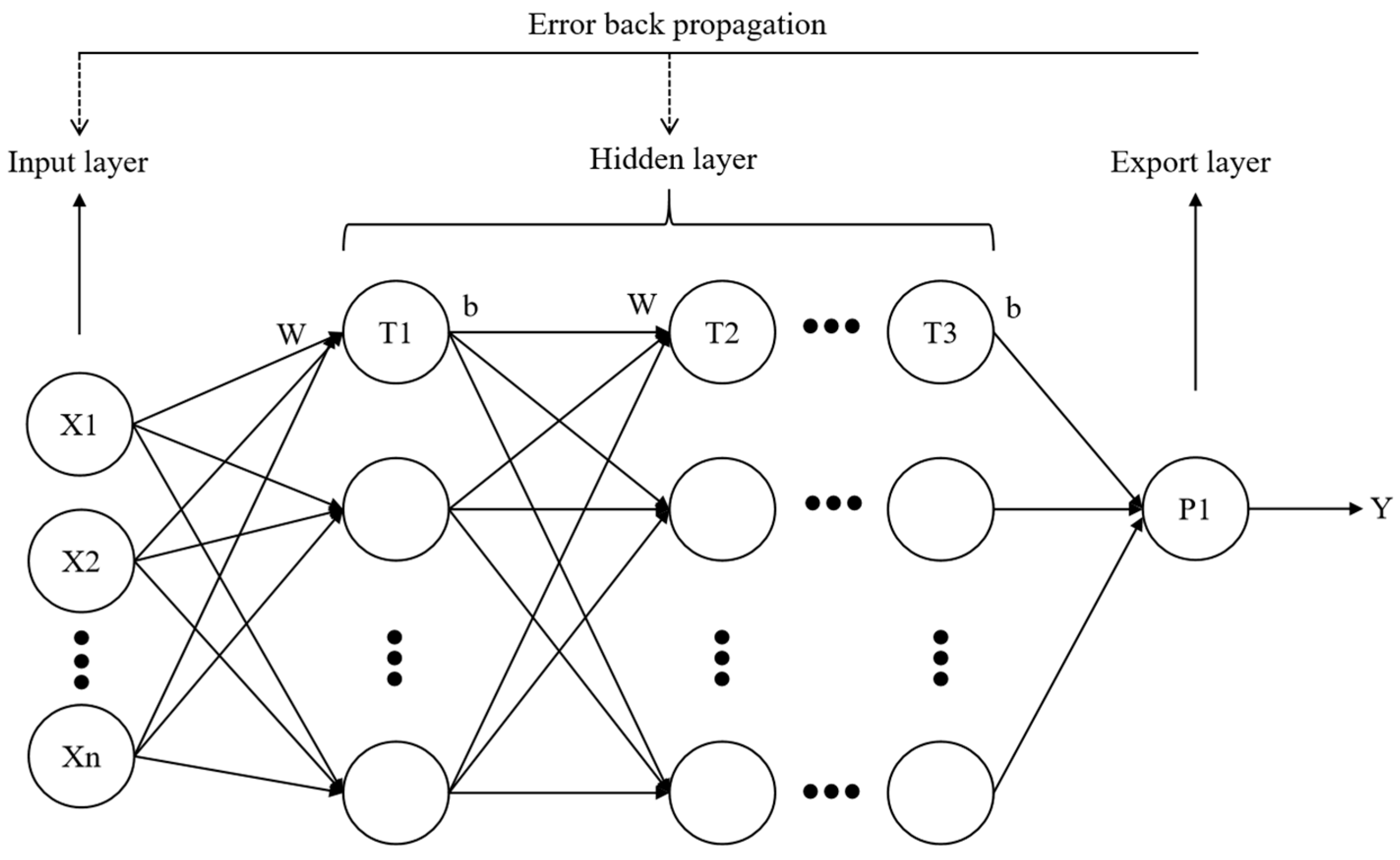
Figure 1. Schematic diagram of BP neural network structure.
Energies 17 04751 g001
Figure 2. Flowchart of the research process in this study.
Energies 17 04751 g002
Figure 4. Brittleness index curves obtained by the mineral method: (a) Z1 well brittleness curves; (b) Z2 well brittleness curves; (c) Z3 well brittleness curves; (d) Z4 well brittleness curves.
Energies 17 04751 g004
Figure 5. Data processing result of well Z1.
Energies 17 04751 g005
Figure 6. Correlation analysis of elastic parameters: (a) brittleness index and Young’s modulus intersection graph; (b) brittleness index and Poisson’s ratio intersection graph; (c) brittleness index and shear modulus intersection graph; (d) brittleness index and bulk modulus intersection graph; (e) brittleness index and Lame constants intersection graph.
Energies 17 04751 g006
Figure 7. Model absolute error analysis with different numbers of hidden nodes.
Energies 17 04751 g007
Figure 8. Correlation analysis between model training data, and test data: (a) correlation analysis between predicted and actual brittleness index of training data; (b) correlation analysis between predicted and actual brittleness index of test data.
Energies 17 04751 g008
Figure 9. Validation analysis of BP neural network model effectiveness: (a) correlation analysis between predicted and real values of brittleness index for Z4 well; (b) comparison of predicted and real values of brittleness index for Z4 well.
Energies 17 04751 g009
Figure 10. Optimization of pre-stack seismic data and fine calibration of well seismic data: (a) CDP gathers; (b) Super CDP gathers; (c) AVA gathers; (d) Z1 well synthetic seismic record.
Energies 17 04751 g010
Figure 11. The plane diagrams of pre-stack simultaneous inversion of elastic parameters data volumes: (a) the plane diagrams of Young’s modulus data volume; (b) the plane diagrams of Poisson’s ratio data volume; (c) the plane diagrams of shear modulus data volume.
Energies 17 04751 g011
Figure 12. The plane diagram of the predicted brittleness index of the BP neural network method.
Energies 17 04751 g012
Figure 13. Comparison plane diagram of the predicted brittleness index results for the target layer in the research area: (a) interpolation distribution plane diagram of the actual brittleness index; (b) brittleness index prediction plane distribution diagram of BP neural network method; (c) brittleness index prediction plane distribution diagram of Rickman method.
Energies 17 04751 g013
Figure 14. Comparison between predicted values and measured values of shale brittleness index seismic prediction based on BP neural network and Rickman method.
Energies 17 04751 g014
Figure 15. Comparative analysis of the brittleness index prediction results: (a) scatter plot of the predicted and true values of the brittleness index; (b) scatter plot of the relative errors of the brittleness index based on the BP neural network and the Rickman method.
Energies 17 04751 g015
Table 1. The absolute error corresponding to the number of hidden layer nodes.
Hidden notes12345
Absolute error0.27030.25250.23610.22890.2256
Hidden notes678910
Absolute error0.20690.19980.19390.20670.2010
Hidden notes1112131415
Absolute error0.19860.18230.20010.19190.1829
Hidden notes1617181920
Absolute error0.17950.17210.16230.16360.1562
Hidden notes2122232425
Absolute error0.15670.15630.15610.15640.1559
Table 2. Partial training datasets and prediction error statistics of BP neural network model.
Sample NumberEμGPredict Brittleness/%Real Brittleness/%Absolute Error/%Relative Error/%
10.1458 0.6267 0.1553 60.57 60.20 0.38 0.62
20.2686 0.5435 0.0879 64.06 63.210.84 1.34
30.2253 0.6031 0.0794 68.02 67.42 0.61 0.90
40.2229 0.6367 0.1061 66.46 67.32 −0.85 −1.27
50.2193 0.6760 0.2043 62.04 53.53 −1.49 −2.35
60.2157 0.6651 0.1267 64.19 55.00 −0.81 −1.24
70.2124 0.6542 0.2116 71.02 48.07 2.95 4.33
80.2136 0.6542 0.1439 60.57 50.53 0.04 0.07
90.2033 0.6338 0.1543 65.52 53.82 1.70 2.67
100.2863 0.4634 0.1378 67.40 49.93 −2.53 −3.61
110.0703 0.6988 0.1995 64.97 59.64 −4.66 −6.69
120.3650 0.6486 0.1299 62.06 66.30 −4.24 −6.39
130.3707 0.6533 0.2305 63.43 66.15 −2.72 −4.12
140.4483 0.4302 0.1319 66.51 61.77 4.74 7.67
150.4159 0.4357 0.1773 66.81 64.69 2.12 3.28
Table 3. Statistical analysis of relative errors in predicting the brittleness index at the well point of the target layer in the research area.
Well ManeActual Brittleness Index/%BP Method of Brittleness Prediction/%Relative Error of BP Method/%Rickman Method of Brittleness Prediction/%Relative Error of Rickman Method /%
Z167.456265.44962.974763.42325.9787
Z266.438968.68343.378369.95845.2973
Z364.096365.82192.692269.34738.1924
Z468.544169.86891.932763.79386.9303
Disclaimer/Publisher’s Note: The statements, opinions and data contained in all publications are solely those of the individual author(s) and contributor(s) and not of MDPI and/or the editor(s). MDPI and/or the editor(s) disclaim responsibility for any injury to people or property resulting from any ideas, methods, instructions or products referred to in the content.