Article

Study on Fast Temporal Prediction Method of Flame Propagation Velocity in Methane Gas Deflagration Experiment Based on Neural Network

1
China Petroleum Safety and Environmental Protection Technology Research Institute, Dalian 116031, China
2
Marine Engineering College, Dalian Maritime University, Dalian 116026, China
*
Author to whom correspondence should be addressed.
These authors contributed equally to this work.
Energies 2024, 17(18), 4747; https://doi.org/10.3390/en17184747
Submission received: 28 July 2024 / Revised: 8 September 2024 / Accepted: 20 September 2024 / Published: 23 September 2024
(This article belongs to the Section I2: Energy and Combustion Science)

Abstract

:
To address the challenges of high experimental costs, complexity, and time consumption associated with pre-mixed combustible gas deflagration experiments under semi-open space obstacle conditions, a rapid temporal prediction method for flame propagation velocity based on Ranger-GRU neural networks is proposed. The deflagration experiment data are employed as the training dataset for the neural network, with the coefficient of determination (R2) and mean squared error (MSE) used as evaluation metrics to assess the predictive performance of the network. First, 108 sets of pre-mixed methane gas deflagration experiments were conducted, varying obstacle parameters to investigate methane deflagration mechanisms under different conditions. The experimental results demonstrate that obstacle-to-ignition source distance, obstacle shape, obstacle length, obstacle quantity, and thick and fine wire mesh obstacles all significantly influence flame propagation velocity. Subsequently, the GRU neural network was trained, and different activation functions (Sigmoid, Relu, PReLU) and optimizers (Lookahead, RAdam, Adam, Ranger) were incorporated into the backpropagation updating process of the network. The training results show that the Ranger-GRU neural network based on the PReLU activation function achieves the highest mean R2 value of 0.96 and the lowest mean MSE value of 7.16759. Therefore, the Ranger-GRU neural network with PReLU activation function can be a viable rapid prediction method for flame propagation velocity in pre-mixed methane gas deflagration experiments under semi-open space obstacle conditions.

1. Introduction

With the development of the times, combustible gases have become an indispensable element in industrial production, daily life, and transportation. However, combustible gases are characterized by their flammability, explosiveness, and difficulty in storage. Incidents of deflagration caused by combustible gas leakage can lead to devastating damage to human lives, the ecological environment, and local economies. Furthermore, as environmental requirements become increasingly stringent, LNG, a clean energy source, has been widely adopted by governments and enterprises. Therefore, it is necessary to conduct pre-mixed methane gas explosion experiments under semi-open space confinement conditions to explore the detailed mechanisms of methane combustion. However, methane combustion experiments are associated with risks, high costs, and limited experimental data acquisition. To address these issues, it is necessary to create a predictive method for rapidly and accurately predicting the process of methane combustion experiments, thereby providing a decision-making basis promptly for emergency response plans in cases of methane gas leakage-induced explosions.
Currently, domestic and foreign scholars primarily use methods such as CFD numerical simulation, empirical formulas, and semi-empirical formulas to study the deflagration experiment process of combustible gases. Zhang [1], in order to delve into the deflagration mechanism of combustible gas clouds on the upper deck of FPSO, conducted numerical simulations of combustible gas cloud deflagration experiments using FLACS software, compared simulation results with experimental data, and used simulation results to reveal the deflagration mechanism of combustible gas clouds on the upper deck of FPSO. Tu et al. [2] used CFD software to simulate and analyze the deflagration experiments of propane in a closed furnace, revealing the deflagration mechanism of propane under medium-to-severe low-oxygen dilution conditions. Holler et al. [3] introduced an improved Eddy Break-Up model into FLUENT simulation software to simulate the deflagration process of hydrogen in a certain safety container. The simulation results show that the accuracy of simulation results decreases as the container width increases compared to real experiments. Wang et al. [4] combined experiments with CFD numerical simulation to reveal the deflagration mechanism of methane–air under the initial turbulent influence. Bassi et al. [5] used OpenFOAM simulation software with the ddtFoam solver to simulate the detonation process of hydrogen in a 5 × 5 × 100 cm3 square pipe, investigating the deflagration mechanism of hydrogen under seven different obstacle configurations. Lei et al. [6] used GASFLOW-MPI simulation software and a four-step hydrogen–methane combustion mechanism model to simulate the deflagration process of hydrogen–methane–air in a 20 L spherical container, exploring the deflagration mechanism of hydrogen–methane–air under different hydrogen concentration conditions. In summary, the use of numerical simulation methods has achieved good research results in the study of deflagration experiments of combustible gases, but the computation time is generally long and cannot achieve rapid and accurate predictions.
To address the issue of rapid and accurate prediction, methods based on neural networks have been widely applied. Shao et al. [7] used a BP neural network optimized by a genetic algorithm to predict the explosion suppression parameters of a vacuum chamber. The prediction results are compared with experimental data, and the effects of vacuum level and flame front position on explosion suppression when diaphragm rupture occurs are also analyzed. Shi et al. [8,9] proposed BRANN neural networks based on artificial bee colony optimization algorithms and transient BRANN neural networks, respectively. Using these two neural networks, the maximum overpressure generated by combustible gas clouds on a marine platform was predicted, and the prediction results were compared with those from cryo-cloud technology and CFD numerical simulations, demonstrating the accuracy and superiority of these network models. Eckart et al. [10] utilized ANN, Support Vector Machine (SVM), Random Forest (RF), and Generalized Linear Regression (GLM) models to quickly predict laminar burning velocity during hydrogen–methane deflagration processes. The prediction results indicated that ANN achieved a high prediction accuracy of around 95%. Stoupas [11] employed a multilayer perceptron to rapidly predict the thermochemical characteristics during methane deflagration processes. The prediction model exhibited high accuracy consistent with the simulation results. It can be seen that previous studies did not predict the overall process of combustible gas deflagration, failing to comprehensively reveal the deflagration mechanism of combustible gases. Therefore, a neural network that can predict data in time series is needed to predict the whole deflagration process of combustible gases.
The Gated Recurrent Unit (GRU) is a type of neural network specialized in predicting time-series data, which can uncover temporal patterns among data and thereby achieve the function of time-series prediction. Pan et al. [12] used the GRU neural network to predict the tailpipe emissions of LNG buses over time; Liang et al. [13] and Jia et al. [14] employed the AdaMax-BiGRU neural network and Adam-GRU neural network to predict the gas concentration in a certain mine, respectively; Xue et al. [15] utilized an attention-based GRU neural network to predict the LNG load of a heating system in a city over time. In summary, although GRU has been widely applied in various fields, few researchers have explored the use of the GRU neural network for predicting the deflagration process of combustible gases over time.
Therefore, a rapid prediction method for pre-mixed methane gas deflagration experiments based on the Ranger-GRU neural network is proposed. This method effectively addresses the issue that conventional pre-mixed methane gas deflagration experiments in semi-open space confinement are costly, challenging, time-consuming, and prone to failure, making it difficult to rapidly and accurately analyze deflagration mechanisms. It also enhances the predictive accuracy of the network model. Moreover, the proposed model does not need to consider the physical and chemical change laws involved in the methane gas deflagration process during the prediction process. Therefore, after expanding the dataset, the same function of fast and accurate prediction of flame speed during the deflagration of different types of combustible gases can be realized. Consequently, it provides decision-making support for emergency response plans to not only methane but also combustible gas deflagration incidents in the shortest possible time. Therefore, when a deflagration accident of methane and other combustible gases occurs, the model can quickly and accurately predict the deflagration process under different scenarios. At the same time, the staff can be based on the model prediction results and quickly and rationally formulate and implement the rapid emergency response plan under the deflagration accident scenario, which greatly improves the efficiency of the emergency scene and reduces the harm caused by the accident.

2. Experimental Introduction

2.1. Experimental System

In order to investigate the deflagration mechanism of premixed methane gas in a semi-open space under the condition of obstacles, and to analyze in detail the influence of obstacles on the flame propagation velocity, an experimental system for the premixed deflagration of methane gas in a semi-open pipeline was constructed.
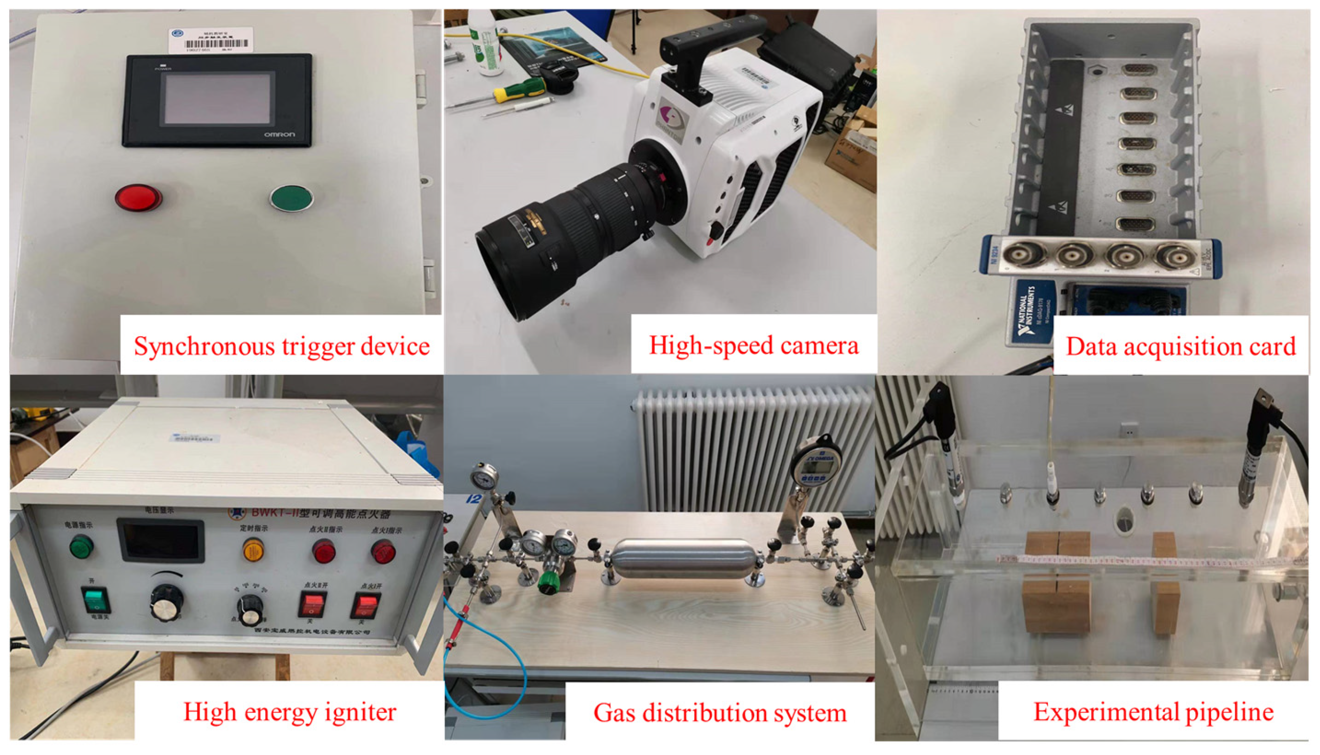
The experimental system consists of five parts: a rectangular experimental pipeline, an ignition device, a data acquisition system, a gas distribution system, and a synchronous triggering system. The rectangular experimental pipeline has an inner diameter of 820 mm × 160 mm × 160 mm, with a wall thickness of approximately 20 mm and a volume of about 21 L. One side of the pipeline is open to release high-temperature gases during experiments, while the other side is used to install the spark plug of the ignition device. The ignition device consists of a spark plug and a high-energy igniter, with an ignition voltage of 60 V and an ignition energy of 100 mJ. The data acquisition system includes pressure sensors, a data acquisition card, and a high-velocity camera. The PPM-127H pressure sensor used was manufactured by Nanjing Hongmu Co., Ltd. in Nanjing, China and has an exposed diaphragm and measuring range from −5 to 5 kPa. The data acquisition card is the Ni9234 card from the National Instruments, Austin, TX, USA. The high-velocity camera is from Phantom series produced by Vision Research, Wayne, NJ, USA. Due to the millisecond-level deflagration velocity of methane–air mixture, the experimental capture velocity is set at 1000 fps, with a camera resolution of 1280 × 800. The synchronous triggering device coordinates the operation sequence of the data acquisition card, high-velocity camera, and high-energy igniter. The gas distribution system consists of gas storage cylinders, digital pressure gauges, gas shut-off valves, pressure-reducing valves equipped with high and low-pressure gauges, and supporting brackets.
The experimental system and equipment are shown in Figure 1 and Figure 2.

2.2. Experimental Procedure

The experimental procedure is as follows: (1) Remove all obstacles and open the threaded hole above the experimental pipeline. (2) Use a fan to exhaust residual gases from the experimental pipeline for 10 min. (3) According to the experimental conditions, position the obstacles in the experimental pipeline. (4) According to Dalton’s law of partial pressures, introduce methane with a volume fraction of 10% into the experimental pipeline. (5) Allow 10 min for thorough mixing of gases to ensure homogeneity. (6) Prepare data acquisition cards, high-velocity cameras, and high-energy igniters controlled by a synchronous triggering device. (7) Trigger the synchronous triggering device to start data acquisition, high-velocity recording, and ignition functions simultaneously. (8) Complete the experiment; repeat steps (1) to (8) for the remaining experimental procedures. Note: to ensure the accuracy of experimental results, each experimental condition should be repeated three to five times.
In accordance with the aforementioned procedure, the steps for methane gas configuration with a 10% volume fraction are as follows: (1) Check the gas tightness of the gas distribution system, replace the gas in the experimental pipeline (21 L) and gas storage cylinder (2.24 L), ensure that the gas in the pipeline is air, and close all valves of the gas distribution system. (2) Evacuate the experimental pipeline to 0.05 MPa vacuum. (3) According to Dalton’s law of partial pressures, introduce air from the air cylinder into the gas storage cylinder until the digital pressure gauge reads 1 MPa, then stop the gas flow. (4) According to Dalton’s law of partial pressures, slowly introduce methane from the methane cylinder into the gas storage cylinder until the digital pressure gauge reads 1.25 MPa, then stop the gas flow. (5) Allow 10 min for the methane–air premixed gas in the gas storage cylinder to mix thoroughly. Then, slowly transfer the gas from the gas storage cylinder into the experimental pipeline until the pressure in the experimental pipeline reaches 0.1 MPa; then, stop. At this point, the methane volume fraction in the experimental pipeline is 10%. Allow another 10 min to ensure a good mixing of gases in the experimental pipeline. (6) Conduct the combustion experiment. (7) After completing the experiment, replace the gas in the experimental pipeline with air. Transfer the remaining premixed gas in the gas storage cylinder into the experimental pipeline until the digital pressure gauge reads 0.25 MPa, then stop the gas flow. (8) Introduce air from the air cylinder into the gas storage cylinder until the digital pressure gauge reads 1.05 MPa, then stop the gas flow. (9) Repeat steps (4) to (5) to prepare methane gas with a 10% volume fraction for the next combustion experiment. Note: except for the first methane gas configuration in the experiment, which includes steps (1) to (5), the subsequent methane gas configurations for experiments follow steps (7) to (9).

2.3. Experimental Conditions

A total of 108 obstacle deflagration experiments under various conditions were conducted, as specified in Table 1.
In the table, VBR, ABR, and P/D represent the volume blockage ratio, area blockage ratio, and spacing-to-equivalent diameter ratio of obstacles, respectively. These three parameters are used to characterize the structure of obstacles. The specific calculation formulas are as follows:
V B R = ( N × D e f f e c t i v e ) 2 × π × H 2 V
A B R = N × D e f f e c t i v e × π × H A s
D e f f e c t i v e = 2 S 2 π 2
P / D = P D e f f e c t i v e
In the equation, N represents the number of obstacles; H is the height of the obstacles, m; V is the volume of the pipeline, m3; A s is the inner surface area of the pipeline, m2; D e f f e c t i v e is the hydraulic equivalent diameter, m; S is the cross-sectional area of the obstacles, m2; and P is the obstacle spacing, m.
The MATLAB 2023b software was used to perform grayscale processing on flame images captured by the high-velocity camera, and the pixel data of the processed flame front was used to calculate flame velocity. Figure 3 shows the flame images before and after grayscale processing. The formula for calculating flame velocity is as follows:
V = L A × B T
In the equation, V is the flame velocity, m/s; L is the actual length of the pipe, m; A is the pixel data corresponding to the end of the pipe; B is the pixel data corresponding to the flame front; T is the time, s.

3. Introduction to Predictive Models

3.1. Introduction to the Network Model

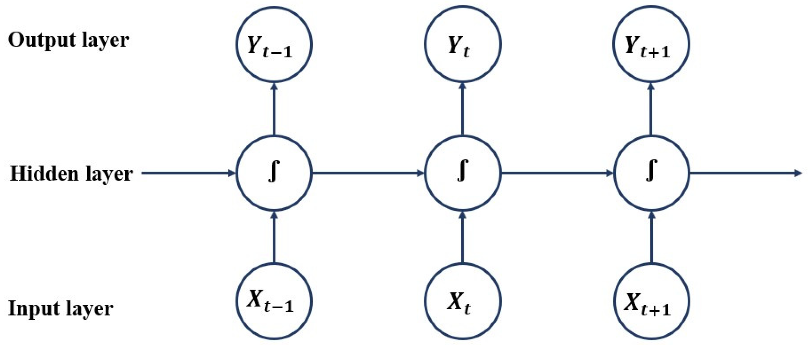
GRU is a type of neural network specifically designed for training on time-series data. Each hidden layer neuron not only connects to neurons in the next layer but also connects with neurons within the same layer. It is this unique network structure that empowers GRU neural networks to predict time-series data. The network structure of GRU is illustrated in Figure 4.
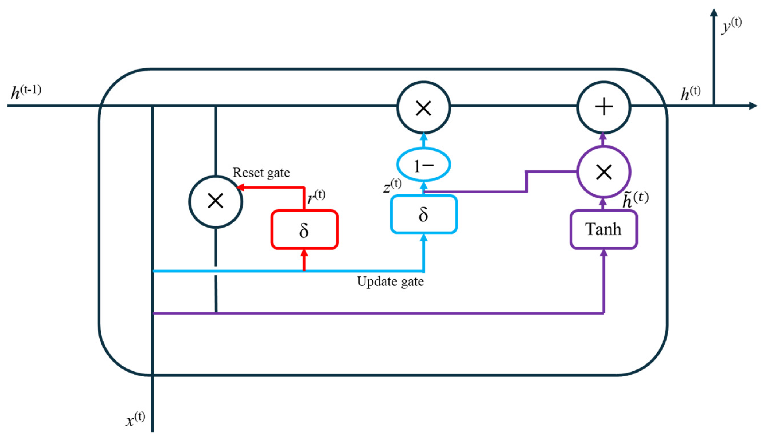
The internal structure of GRU neurons includes two gate control units: the reset gate and the update gate. These two gate control units, respectively, decide whether to keep or discard information passed from the previous time step and select retained information again to update the current neuron state. The internal structure diagram of the neuron is shown in Figure 5.
The update gate math formula:
z t = σ ω z h t 1 + U z x t + b z
The reset gate math formula:
r t = σ ω r h t 1 + U r x t + b r
The formula for computing candidate information passed to the next time step neuron:
h ~ t = Tanh ω h r t h t 1 + U h x t + b h
The formula for calculating the output value of the neuron and the information carried by the data when the neuron is transmitted to the next moment:
y ( t ) = h t = 1 z t h t 1 + z t h ~ t
In the formula, z t and r t , respectively, represent the update gate and reset gate; h ~ t stands for candidate information; y ( t ) and h t represent the current time step neuron output value and the information carried when passed to the next time step neuron; ω z , ω r , ω h , U z , U r , and U h denote the weights for the two gate control units and computation of candidate information; b z , b r , and b h are the thresholds for the two gate control units and computation of candidate information.
A Recurrent Neural Network (RNN) is a neural network specialized in training time-series data, and its hidden layers are connected to neurons in the same way as GRU. However, there is no gate control unit structure inside its neurons, so it is unable to memorize the information between time-series data over longer time intervals.
Similarly to GRU, the Long Short-Term Memory (LSTM) neural network neurons also have the same internal structure of gate control units, but there are three gate control units, which are the forgetting gate, input gate, and output gate. Therefore, compared with GRU, although it can also process the memorized information between time-series data over a longer time interval, its computational efficiency may be reduced due to the increase of gate control units.

3.2. Introduction to the Activation Function

To optimize the predictive capability of the GRU neural network, three types of activation functions are compared: Sigmoid, ReLU, and PReLU. The descriptions of these three activation functions are as follows:
The Sigmoid activation function is a saturating activation function that can control the magnitude of weight updates during the backpropagation process of neural networks and restrict the output values of the activation function within the boundary range of 0–1, thereby preventing input data from becoming too dispersed during training [16]. Additionally, the Sigmoid activation function can enhance the neural network’s non-linear fitting capability, enabling the network to fit more complex data. The specific mathematical formula of the Sigmoid activation function is shown below:
f x = 1 1 + e x
The ReLU activation function is a non-saturating function that helps mitigate the gradient vanishing problem in neural networks, while also enhancing the numerical stability of the network. Additionally, it can restrict the output values of the activation function within the boundary range of 0–1 [16]. The specific mathematical formula of the ReLU activation function is shown below:
f x = max 0 , x
The PReLU activation function is an improvement over the Relu activation function, allowing for computation and corresponding gradients for inputs and outputs less than 0 during the backpropagation process of neural networks. Additionally, the random noise in the PReLU activation function assists in updating the weights and thresholds of each hidden layer neuron during the network’s backpropagation process, using features extracted from methane combustion experimental data. This helps the neural network address local optima issues that may arise during updates [17,18]. It is noteworthy that the random noise in the PReLU activation function can adjust automatically based on different neurons [17]. The specific mathematical formula of the PReLU activation function is shown below:
f x = x   x > 0 α x   x 0
In the formula, f x represents the hidden layer output value; x denotes the hidden layer input value; and α is a random noise parameter, with values ranging from 0 to 1.

3.3. Introduction to the Optimizer Model

To further enhance the robustness and predictive capability of the GRU neural network, four new types of optimizers—Adam, Lookahead, RAdam, and Ranger—were selected for comparison.
The Adam optimizer has advantages such as high computational efficiency, adaptive learning rate adjustment, insensitivity to hyperparameters, etc., which effectively enhance the predictive capability of neural networks [19]. The update process of weight parameters using the Adam optimizer is shown in the following equation:
g t θ f t θ t 1
m t β 1 m t 1 + 1 β 1 g t
v t β 2 v t 1 + 1 β 2 g t 2
m ~ t m t 1 β 1 t
v ~ t v t 1 β 2 t
θ t θ t 1 α m ~ t v ~ t + ε
Among them, t represents the time step; g t denotes the gradient of the objective function; θ stands for the neural network weight parameters; f t ( θ ) is the objective function; m t and v t are the first and second-moment estimates of the update indices; β 1 and β 2 are the exponential decay rates for the first and second-moment estimates; m ~ t and v ~ t are the bias-corrected first and second-moment estimates, respectively; α represents the learning rate; and ε is a small constant.
The Lookahead optimizer consists of two internal optimizers: the Lookahead optimizer itself and a conventional optimizer (such as SGD or Adam). The conventional optimizer is used for pre-searching and selecting the direction of weight parameter updates, while the Lookahead optimizer performs more refined training and optimization of the weight parameters based on the pre-selected direction. This optimizer addresses issues such as slow convergence and low prediction accuracy observed with SGD [20]. The update process of weight parameters using the Lookahead optimizer is shown in the following equation:
θ t , 0 t 1
θ t , i θ t , i 1 + A L , θ t , i 1 , d
t t 1 + α θ t , k t 1
Among them, θ represents the weights of the conventional optimizer; denotes the weights of the Lookahead optimizer; A is the conventional optimizer; L is the objective function of the conventional optimizer; d is the training dataset of the neural network; α is the learning rate for the weights of the Lookahead optimizer; and k is the synchronization period between the Lookahead optimizer and the conventional optimizer.
The RAdam optimizer employs a Warm-up method to address the issue of Adam optimizer’s susceptibility to local minima. Additionally, it features advantages such as fast computation velocity and reduced dependency on learning rate, demonstrating good accuracy and robustness during training [21]. The update process of weight parameters using the RAdam optimizer is shown in the following equation:
g t θ f t θ t 1
v t 1 β 2 v t 1 + 1 β 2 g t 2
m t β 1 m t 1 + 1 β 1 g t
m ~ t m t 1 β 1 t
β t β 2 t β 2 t 1 β 2 t
When ρ t > 4 :
l t 1 β 2 t v t
r t ρ t 4 ρ t 2 ρ ρ 4 ρ 2 ρ t
θ t θ t 1 α t r t m ~ t l t
When ρ t 4 :
θ t θ t 1 α t m ~ t
In the equation, ρ t represents the variance; l t denotes the adaptive learning rate; r t is the differential correction term; and α t stands for the time step. For explanations of the remaining parameters, refer to the parameter meanings described in Equations (13)–(18).
The Ranger optimizer possesses advantages such as fast convergence velocity, insensitivity to hyperparameters and learning rate, resistance to local minima, and reduced likelihood of missing global optima. Moreover, it demonstrates good stability and accuracy during training, effectively enhancing the predictive capability of neural networks.

3.4. Introduction to Evaluation Indicators

The coefficient of determination R2 is chosen as the evaluation metric for the network model. R2 provides a comprehensive assessment of the overall prediction error of the network model and reflects the degree of adaptation between predicted values and actual values. The specific mathematical formula of R2 is shown below:
R 2 = 1 i = 1 n y ~ i y i 2 y ¯ y i 2
In the formula, y represents the actual data values; y ~ denotes the output values from the neural network; and y ¯ signifies the mean of the data.
The mean squared error (MSE) is selected as the evaluation metric for the network model, and MSE can be used to measure the degree of difference between predicted values and actual values. The specific mathematical formula of MSE is shown below:
M S E = 1 m i = 1 m y ~ i y i 2
In the formula, m represents the total number of data points, while the meanings of other parameters can be found in the parameter definitions provided in Equation (31).

3.5. Introduction to Proposed Model

The structure of the proposed model is shown in Figure 6.
The proposed model consists of the GRU neural network, PReLU activation function, and Ranger optimizer. Firstly, the input data need to be preprocessed in three-dimensional temporal order according to the set GRU time step, which allows the GRU to extract the input data in chronological order during the training period. Second, the input data will enter the GRU neural network for operation, and the Ranger optimizer will adaptively adjust its own learning rate according to the results of the forward propagation during the backpropagation of the network in order to help the GRU find the optimal weights and thresholds value. Finally, when the prediction results do not reach the target accuracy, the input data will be re-input into the GRU for a new round of calculation. When the prediction results reach the target accuracy, GRU will end the training and output the prediction results.

4. Analysis of Experimental and Predicted Results

4.1. Analysis of Experimental Results

The purpose of this section is to analyze the influence of obstacles on flame velocity during the deflagration process of methane under different conditions, including different lengths, shapes, distance from the ignition source, spacing, and thickness of barbed wire obstacles. The results of the analysis can be judged whether the predictions of the model are reasonable or not.

4.1.1. The Effect of the Distance of the Obstacle from the Ignition Source

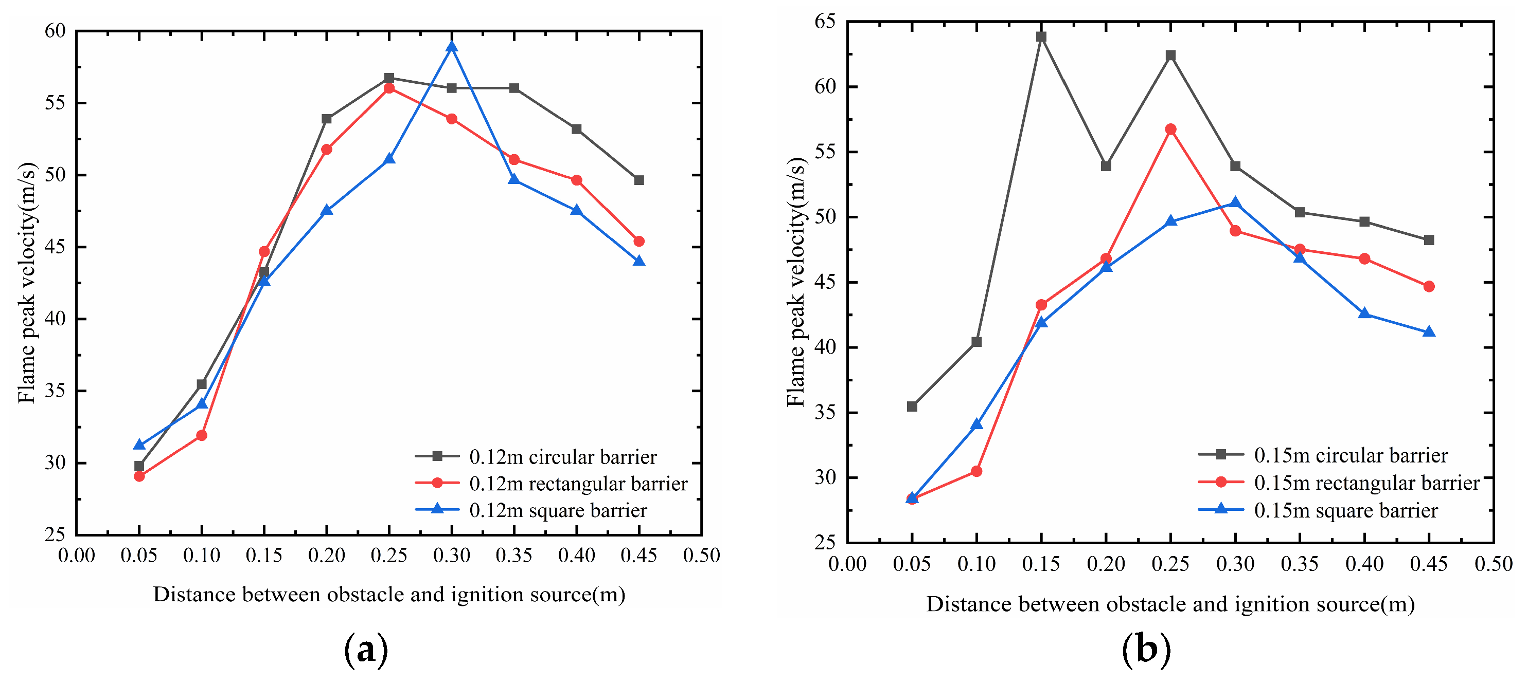
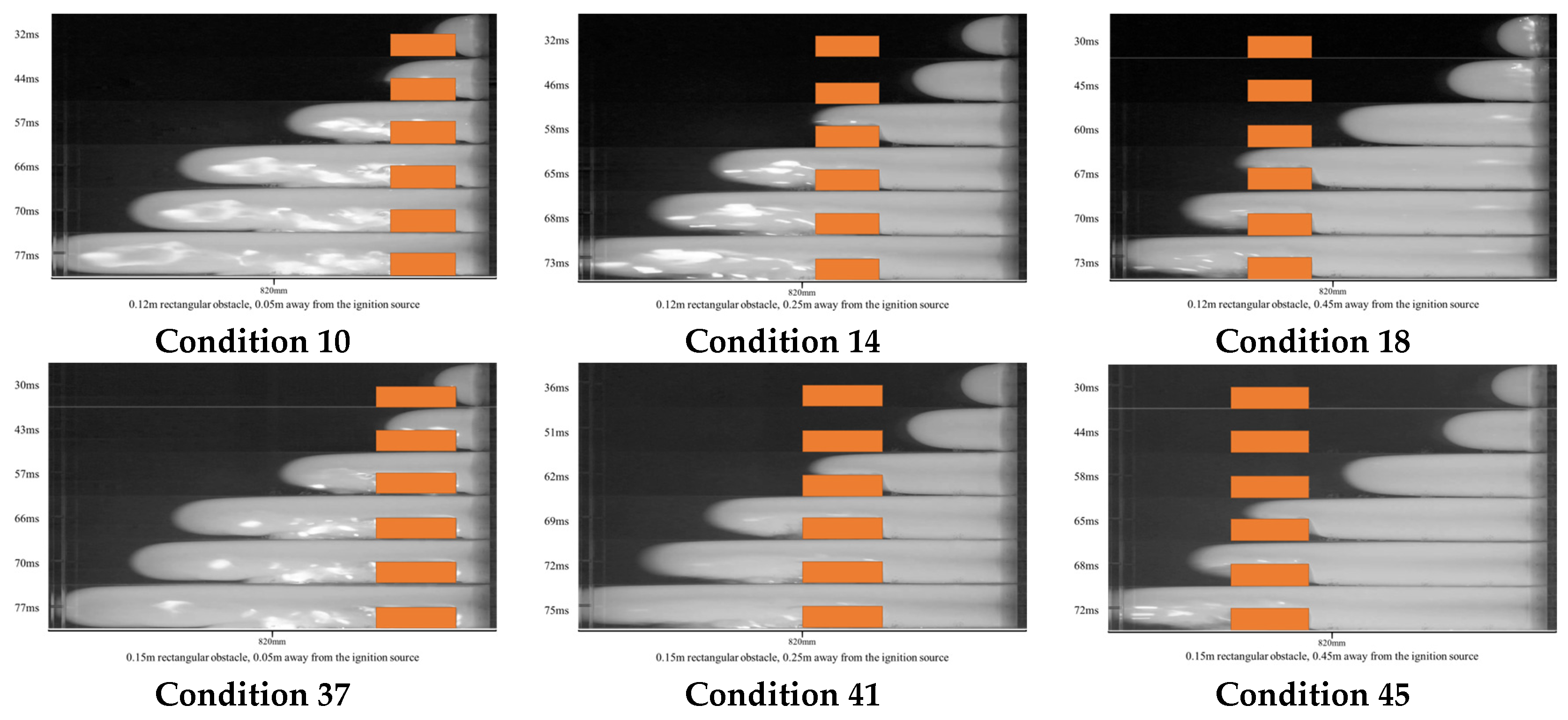
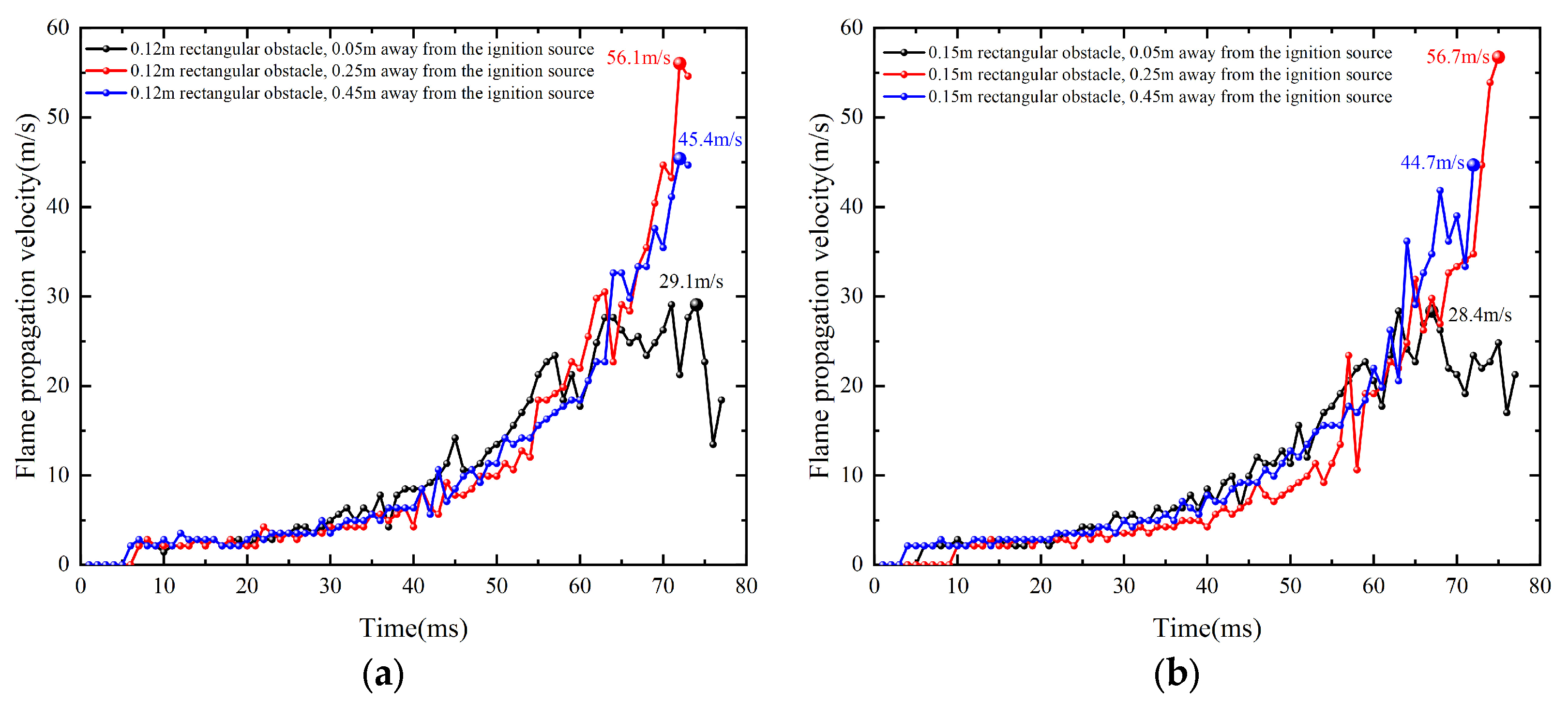
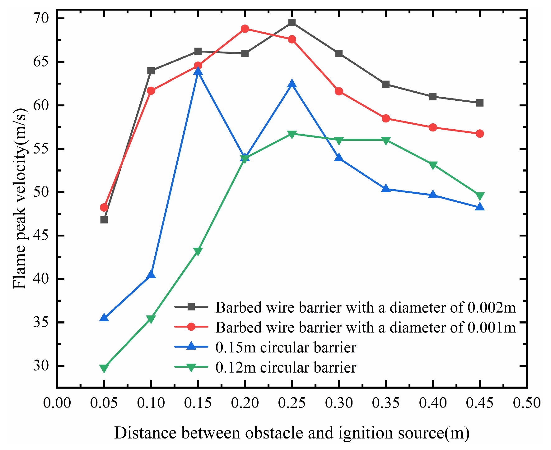
As shown in Figure 7, Figure 8 and Figure 9, when the obstacle is positioned closer to the ignition source, the flame is prematurely subjected to induced turbulence caused by the obstacle. The increased flame pressure pushes unburned gas out of the pipeline, leading to a reduction in the peak flame velocity. As the distance between the obstacle and the ignition source increases, the flame velocity increases before the flame contacts the obstacle, and the turbulence effect is intensified upon the contact, resulting in an increase in peak flame velocity. When the obstacle is placed further from the ignition source, the time for the flame to be accelerated by turbulence after contacting the obstacle is shortened, and the flame is released from the pipeline outlet before it has time to be fully accelerated, resulting in a reduction of the peak flame velocity. Therefore, when the obstacle is approximately 0.25 m from the ignition source, the peak flame velocity is at maximum. Additionally, during flame propagation, pressure waves generated by combustion rebound upon contacting the pipeline wall and obstacle, hindering the flame propagation process and disturbing the flame burning velocity. When the flame propagates to the end of the pipe, the contact area of the pressure wave with the wall is reduced. As the flame passes over the obstacle, the perturbation effect of the pressure wave on the flame burning speed is weakened. Consequently, the flame burning velocity begins to converge to normal, which ultimately leads to changes in the flame burning velocity and inconsistencies in the peak flame velocity. Similar phenomena can be observed in other operating conditions.

4.1.2. The Effect of the Shape of the Obstacle

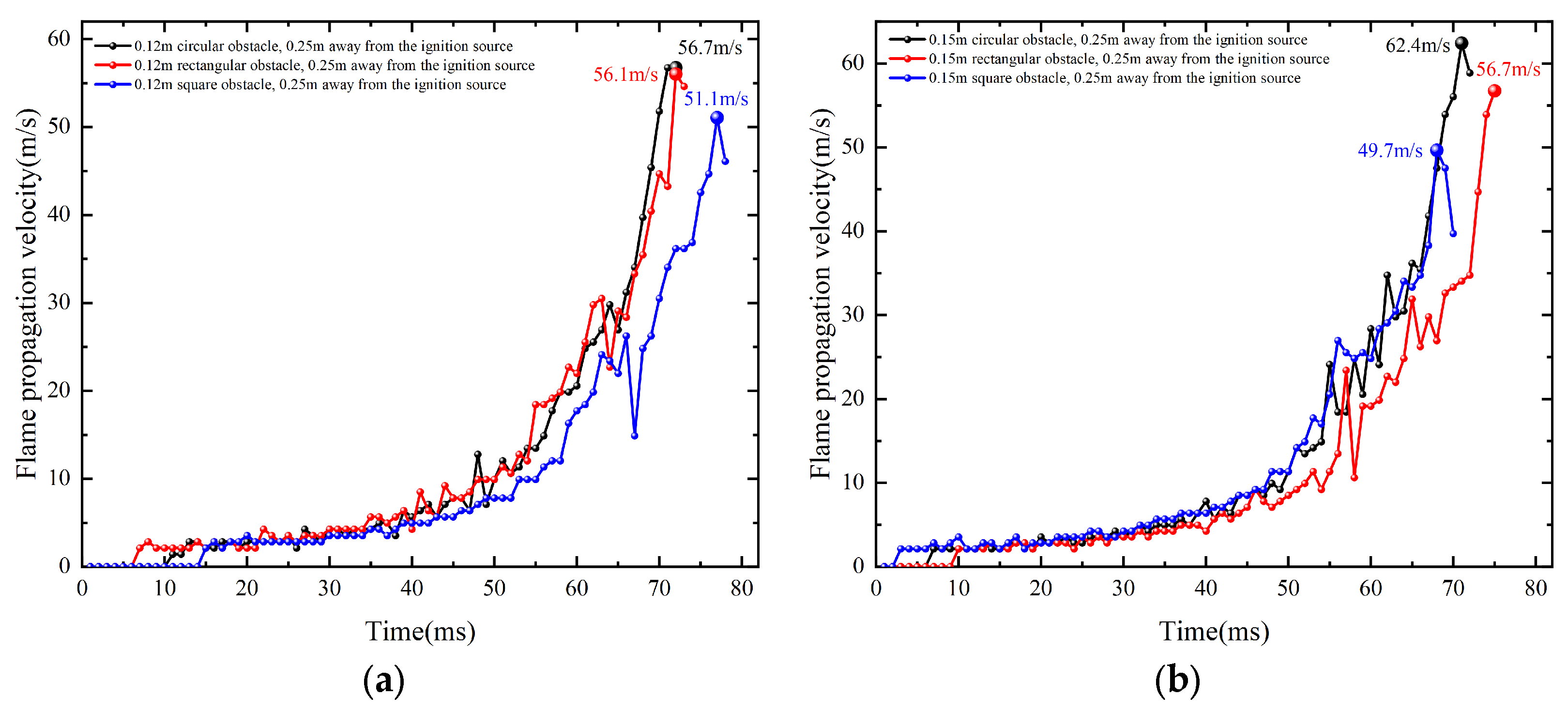
As shown in Figure 10 and Figure 11, due to the minimal distance between the surface of the cylindrical obstacle and the top of the experimental pipeline, an irregular arc-shaped channel is formed between the obstacle and the experimental pipe wall. In contrast to the regular-shaped channels formed between rectangular and square obstacles and the pipe wall, when the flame passes above the cylindrical obstacle, pressure waves induce stronger turbulent effects on the unburned gases. This results in the peak flame velocity being higher for the circular obstacle condition compared to the rectangular and square obstacle conditions.

4.1.3. The Effect of the Obstacle Spacing

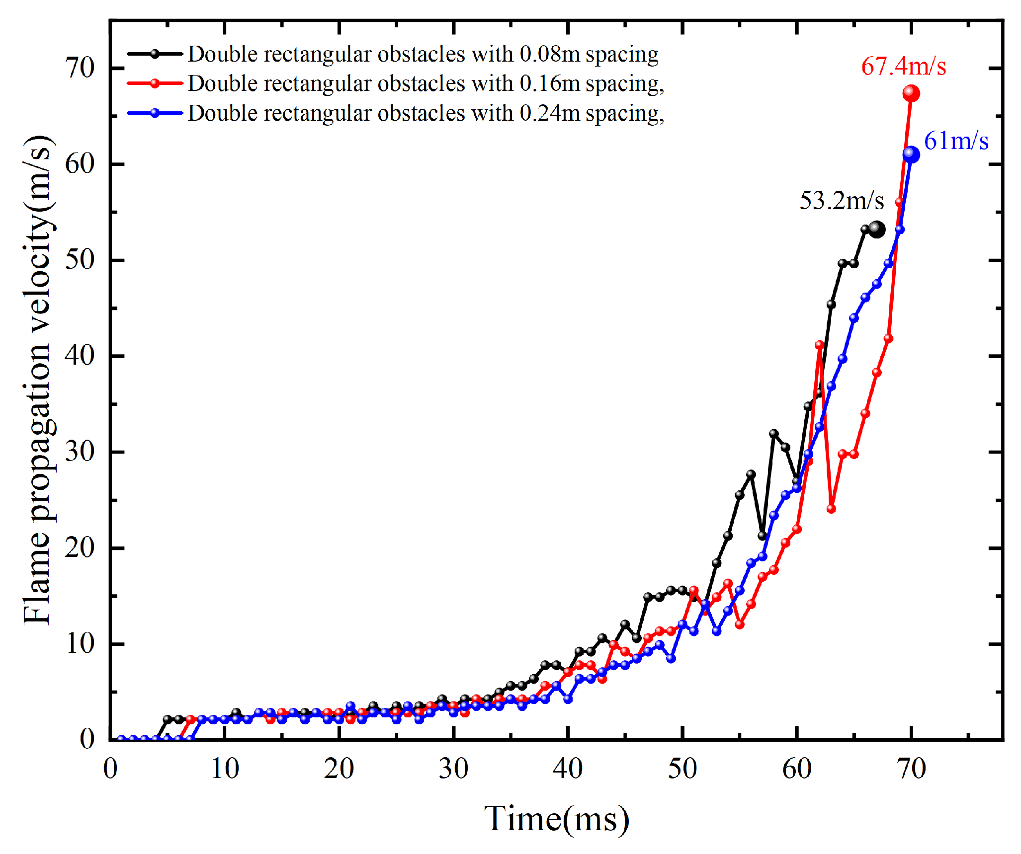
As shown in Figure 12, Figure 13 and Figure 14, when the flame contacts the first obstacle, it is initially subjected to the induced turbulence effect of the obstacle, which subsequently accelerates the flame burning velocity. When the distance between the two obstacles is 0.08 m, the flame is subjected to the turbulence effect of the second obstacle due to the close spacing between the obstacles. The increased pressure wave pushes most of the unburned gas out of the pipe, ultimately leading to a decrease in the peak flame velocity. When the distance between the two obstacles is 0.16 m, the flame has already fully accelerated. Upon encountering the turbulence effect of the second obstacle again, the flame continues to accelerate and ignites more unburned gas ahead, resulting in an increase in flame acceleration and ultimately a higher peak flame velocity. When the distance between the two obstacles is 0.24 m, the flame’s acceleration tends to stabilize upon reaching the second obstacle. With less unburned gas remaining in the pipe, the flame acceleration changes little, leading to a decrease in the peak flame velocity. Therefore, as the distance between obstacles increases, the peak flame velocity first increases and then decreases. The trend of peak flame velocity with obstacle spacing is generally consistent for obstacles of different shapes.

4.1.4. The Effect of the Barbed Wire Obstacle

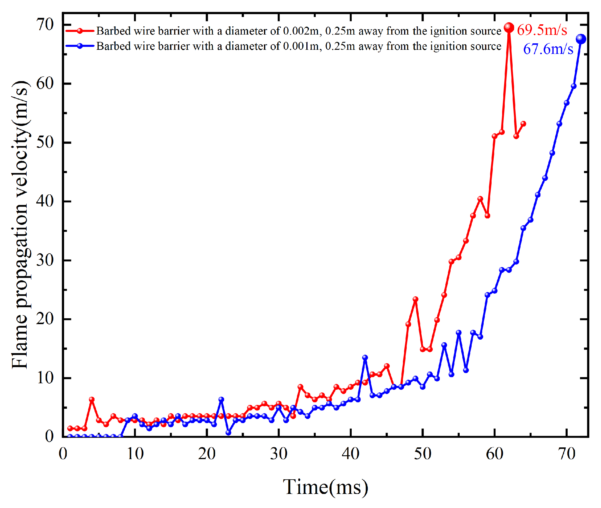
For the barbed wire obstacle, the diameters are 1 mm and 2 mm, and the length, width, and height of them are 0.12 m. As shown in Figure 15, Figure 16 and Figure 17, the barbed wire obstacle with a 1 mm diameter has more layers, resulting in a denser structure that increases the contact area with the flame. This dense structure causes more reflections of pressure waves upon contact with the surface of the 1 mm wire mesh. Additionally, the good thermal conductivity of the barbed wire obstacle allows the 1 mm diameter barbed wire obstacle to absorb more heat, preventing the complete ignition of the premixed gas behind it, and leading to flame quenching. The 1 mm-diameter barbed wire obstacle also has a finer three-dimensional porous structure, acting as a porous medium that rapidly attenuates the propagation of explosion waves. Consequently, the peak flame velocity under the 1 mm diameter barbed wire obstacle is lower than that under the 2 mm diameter barbed wire obstacle.
Observing the flame shapes around the barbed wire obstacle and the circular obstacle, it is noted that as the flame passes through the barbed wire obstacle, the flame front changes from “finger-shaped” to “spinelike-shaped” as it progresses forward. This transition is accompanied by intense turbulence that accelerates the flame, resulting in a higher peak flame velocity under the barbed wire obstacle condition compared to the circular obstacle.
As shown in Figure 3, the calculation of flame velocity requires the use of more complex software and algorithms to carefully process the images captured by the high-speed camera. And after the processing is completed, it is also necessary for the researcher to calculate the flame velocity per millisecond according to the processed image and the formula. However, due to the different standards of judgment of each researcher, there will be a large or small error in the calculation process. Therefore, the calculation process of flame velocity will not only consume a lot of time and labor but is also highly prone to errors. In view of this, the flame velocity will be predicted next to reduce the complexity and improve the accuracy of the flame velocity calculation.

4.2. Prediction Results Analysis

4.2.1. Datasets and Neural Network Models

The experimental data of premixed methane gas deflagration in semi-open space with obstacles were selected as the dataset for training the neural network. As indicated in Section 4.1, the shape, spacing, and distance of obstacles from the ignition source all affect the flame velocity. The values of VBR, ABR, and P/D are determined by the shape and spacing of obstacles. Therefore, VBR, ABR, and P/D for 11 different types of obstacles and nine different ignition source distances were chosen as input vectors for the neural network.
As indicated in Section 2.3, the handling and calculation process of flame velocity requires significant human effort and time, while flame pressure can be measured simply by connecting a pressure sensor. Therefore, this paper selects flame velocity from deflagration experiments as the output vector for the neural network.
The network’s hidden layer count was set to 1, the step size to 6, the learning rate to 0.002, and the training iteration count to 500 times. The dataset comprises 108 sets of conditions totaling 6372 data points. Condition 2, 9, 13, 26, 31, 37, 50, 58, 60, 65, 70, 72, 75, 81, 85, 90, 93, and 106 were randomly selected as the test set, with the remaining ninety sets used as the training set, resulting in a training-to-set ratio of 5:1. The dataset files can be downloaded from Supplementary Materials.
To ensure the credibility of the prediction results of the proposed model, 10 consecutive predictions were made for each test, and the R2 and MSE mean value and the degree of dispersion of the 10 prediction results were used as the judgment indexes of the prediction ability and accuracy of the model.

4.2.2. Sensitivity Analysis of the Number of Neurons

Because the prediction accuracy of the neural network no longer shows a significant increase after a certain number of neurons, as the number of neurons increases, the computational efficiency of the neural network begins to decrease [22,23]. Thus, sensitivity analysis for the number of neurons was performed in this section.
The number of neurons was set to 4, 8, 12, 16, 20, 24, 28, and 32, respectively, and these values were applied to train the RNN, LSTM, and GRU neural networks. The predicted results and their trends are depicted in Table 2 and Figure 18.
As shown in Table 2 and Figure 18, the R2 mean value for the RNN, LSTM, and GRU neural networks all exhibit a significant improvement when the number of neurons is set to 24 in the hidden layer. Beyond 24 neurons, the R2 mean value tends to stabilize. Therefore, the hidden layer neuron count for all three neural networks is set to 24.

4.2.3. Comparative Analysis of Neural Network Models

RNN, LSTM, and GRU all can predict temporal data. RNN is characterized by high prediction efficiency. LSTM is characterized by strong memory, high prediction accuracy, robustness, and no gradient disappearing problem due to the existence of three different gate control units inside the neurons. GRU has higher prediction efficiency compared to LSTM due to its simplified neuron internal structure, but its prediction accuracy may be reduced compared with LSTM. Therefore, to evaluate the prediction performance of the three neural networks in detail, the RNN, LSTM, and GRU neural networks were trained. During the training process, the number of neurons for the three neural networks was set to 24, the activation function was set to Sigmoid, and the optimizer was set to SGD; a neural network with the best prediction ability was selected as the prediction model by comparing the prediction value distribution, trend prediction, R2 mean value, and MSE mean value of the test set of the three neural network models.
As shown in Table 3 and Table 4, as well as Figure 19 and Figure 20, the predicted values of the RNN neural network largely deviate from the 25% error range, with many values exceeding the 50% error range. Overall, the predicted trend only partially matches the true trend, particularly in the lower range of true values. The R2 mean value is the lowest with the largest fluctuation, while the MSE mean value is the highest with significant variability. For the LSTM neural network, although most predicted values also deviate beyond the 25% error range, compared to RNN, fewer predictions exceed the 50% error range. The overall predicted trend shows a slight improvement in alignment with the true trend, especially in the lower range of true values. The R2 mean value improves with increased fluctuation, while the MSE mean value decreases but with increased variability. Similarly, for the GRU neural network, although most predicted values deviate beyond the 25% error range, compared to RNN and LSTM, fewer predictions exceed the 50% error range. The overall predicted trend shows a slight improvement in alignment with the true trend, particularly compared to LSTM. The GRU has the highest R2 mean value with the lowest fluctuation and the smallest MSE mean value with the lowest variability. Based on these observations, GRU was selected as the neural network prediction model for this study.

4.2.4. Comparative Analysis of Activation Functions and Optimizers

The combination of different activation functions and optimizers with neural networks can enhance the predictive capabilities of the network to varying degrees. To optimize the prediction performance of the GRU, a comparative analysis of the activation functions and optimizers used was conducted.
Activation function comparative analysis: the Sigmoid activation function is a saturating function, while Relu and PReLU activation functions are non-saturating functions. Moreover, Relu outputs zero for negative input values; thus, its output capability is limited compared to PReLU. Therefore, three activation functions—Sigmoid, Relu, and PReLU—are applied to the GRU neural network for training. By comparing the distribution of predicted values, trend predictions, and the R2 mean value and MSE mean value on the test set, the most compatible activation function with the GRU neural network was selected.
As shown in Table 5 and Table 6 and Figure 21 and Figure 22, when the activation function is Sigmoid, almost all predicted values fall outside the 25% error interval. Compared to the true trend, only a few predictions align. The R2 mean value is the lowest with the largest fluctuation, and the MSE mean value is the highest with the greatest fluctuation. When the activation function is Relu, predictions within the 25% error interval notably increase, though many values still exceed this range. Overall, most predictions align well with the true trend. The R2 mean value significantly improves with the lowest fluctuation, and the MSE mean value decreases noticeably with the lowest fluctuation as well. With PReLU as the activation function, the majority of predictions are within the 25% error interval. Compared to Sigmoid and Relu, there are fewer predictions outside this range. Most predictions align well with the true trend and, particularly within the range of true values from 30 to 50, the alignment improves notably compared to Relu. The R2 mean value is the highest with a moderate fluctuation, and the MSE mean value is the lowest with a moderate fluctuation. Therefore, PReLU was chosen as the activation function for GRU.
Optimizer comparison analysis: the Adam optimizer primarily optimizes the training process of neural networks by adaptively adjusting the learning rate. The Lookahead optimizer enhances the search and selection of learning rates during neural network training. The RAdam optimizer focuses on optimizing the selection of initial learning rates for neural networks, while the Ranger optimizer optimizes the entire training process of learning rate selection. To compare the performance of these four optimizers—Adam, Lookahead, RAdam, and Ranger—they were applied to a GRU neural network with PReLU activation function. By comparing the distribution of predicted values, trend predictions, the R2 mean value, and the MSE mean value on the test set, the optimizer that exhibits the best performance was selected for use.
As shown in Table 7 and Table 8, as well as Figure 23 and Figure 24, when the optimizer is Lookahead, most predicted values are within a 25% error range, with fewer predictions within a 10% error range. Overall, the predicted trends mostly align with the true trends. The R2 mean value is the lowest with the highest fluctuation, and the MSE mean value and fluctuation are also the highest. When the optimizer is RAdam, most predicted values are within a 25% error range, and there is a noticeable improvement in predictions within a 10% error range compared to Lookahead. The overall predicted trends align well with the true trends, with significant improvements observed in the alignment in the 0–10 and 50–60 ranges compared to Lookahead. The R2 mean value increases, and both R2 and MSE fluctuations decrease. For the Adam optimizer, predictions within 25% and 10% error ranges show improvement compared to RAdam. The overall predicted trends align well with the true trends, with slight improvements in alignment observed in the 40–60 range compared to RAdam. The R2 mean value shows a slight increase, and both R2 and MSE fluctuations decrease. With the Ranger optimizer, almost all predicted values are within a 25% error range, with a majority within a 10% error range. The overall predicted trends align closely with the true trends, except for a few areas in the 45–60 range where there is partial alignment. The R2 mean value is the highest, with the lowest fluctuation, and both MSE mean value and fluctuation are also the lowest. As shown in Table 9 and Table 10, when the optimizer is Ranger, the R2 and MSE mean values of the training set are higher and lower than those of the test set, but the differences are not significant. This indicates that the proposed model does not suffer from overfitting. In addition, it can be seen that the dispersion of the R2 and MSE values obtained from the ten predictions of the training and test set is not large, where the dispersion ranges of R2 are 0.00572 and 0.00264 and the dispersion ranges of MSE are 0.85313 and 0.75461, which indicates that the proposed model has strong robustness in the process of predicting the data for the training set and the test set.
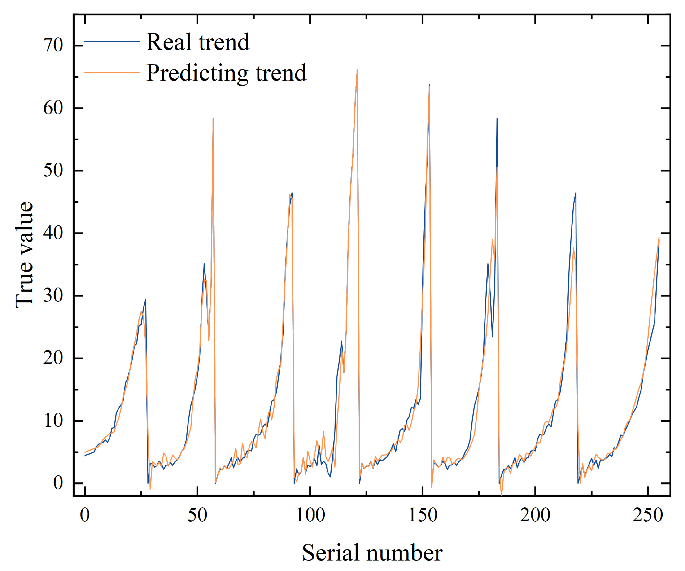
In addition, to further validate the prediction performance of the proposed model, time-series predictions were made for the flame propagation velocity data of part of the methane deflagration experiments conducted by Zhang et al. [24]. The prediction results are shown in Table 11 and Figure 25.
As shown in Table 11 and Figure 25, the prediction model based on the PReLU activation function, Ranger optimizer, and GRU neural network demonstrates high accuracy in predicting flame propagation velocity in the methane deflagration experiments conducted by Zhang et al. [24]. Specifically, the model achieves an average R2 value of 0.96284 and an average MSE of 6.14896. Except for a few values with prediction errors, the predicted values are generally consistent with the real value. Therefore, it can be concluded that the model has high predictive accuracy.

4.2.5. Analyzing the Influence of Input Vectors on Prediction Results

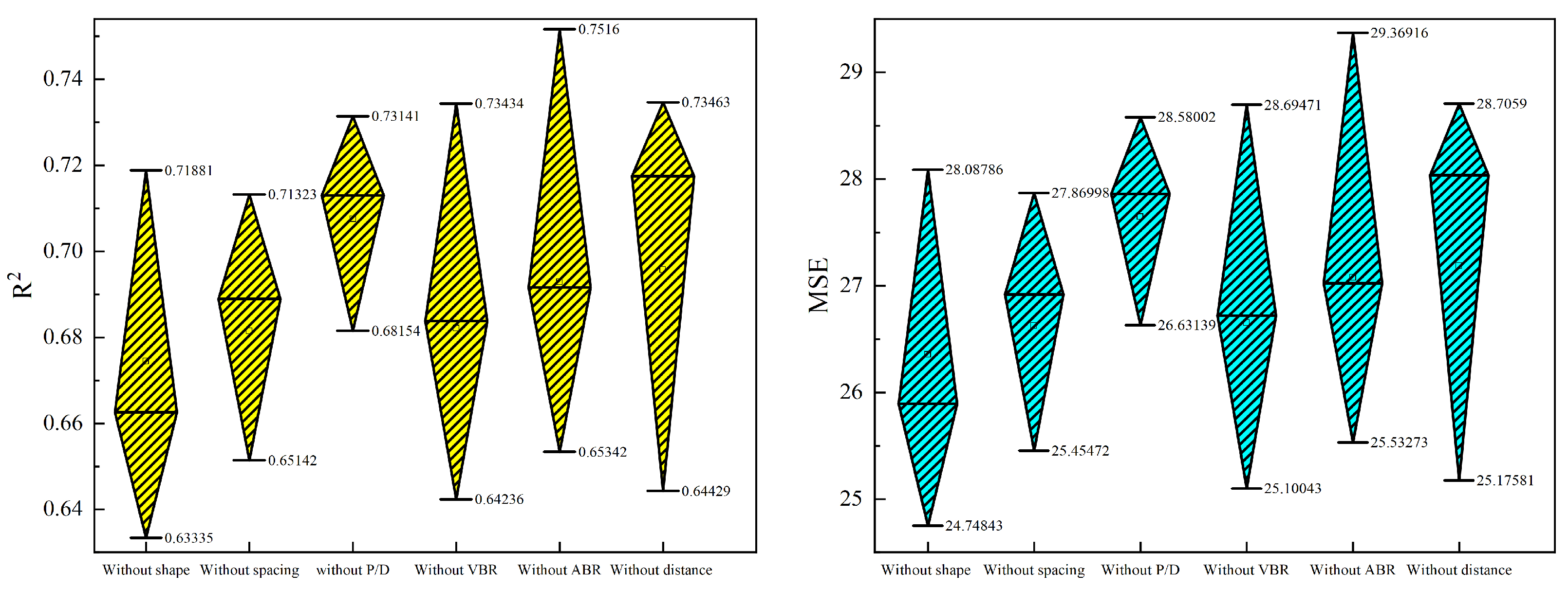
To ensure that the selected seven input vectors significantly impact the prediction accuracy of the proposed model, a detailed analysis of the influence of these input vectors on the prediction results was conducted. First, one category of input vectors was removed from the dataset each time. Then, the model was trained and tested using the remaining input vectors. Finally, based on the R2 and MSE values obtained from the test set, the impact of each input vector on the prediction results was analyzed.
As shown in Table 12 and Table 13 and Figure 26, when a certain category of input vectors is deleted, the mean value of R2 and MSE decreases and increases, respectively, due to the reduction in the number of features. In addition, regardless of which class of input vectors is deleted, the mean values of R2 and MSE for the test set are similar, and there is little difference in the range of discretization. Therefore, all seven input vectors selected significantly affect the prediction accuracy of the model, and each type of input vector has almost the same degree of influence on the prediction results.

5. Conclusions

(1)
A prediction method based on the PReLU activation function, Ranger optimizer, and GRU neural network was developed to predict the experimental process of premixed methane gas deflagration under semi-open space obstacle conditions for the first time.
(2)
A total of 108 sets of methane deflagration experiments under semi-open obstacle conditions were conducted. The experimental results indicate that both excessively large or small distances between obstacles and the ignition source, as well as excessively large or small distances between obstacles, can reduce the peak flame velocity. The shape of obstacles affects the peak flame velocity. The specific structure of wire mesh obstacles can lead to quenching phenomena, and finer wire mesh exacerbates the negative impact on the peak flame velocity caused by quenching phenomena.
(3)
The prediction results show that the Ranger-GRU neural network based on the PReLU activation function achieves an R2 mean value of 0.96164 and a MSE mean value of 7.16759. Compared to the RNN, LSTM, and GRU neural networks, the R2 mean value improved by 93.7%, 84.4%, and 71.2%, respectively, while the MSE mean value decreased by 92.4%, 92%, and 91.2%, respectively. Compared to GRU neural networks with Sigmoid, ReLU, and PReLU activations, the R2 mean value improved by 71.2%, 16.3%, and 11%, respectively, while the MSE mean value decreased by 91.2%, 77.8%, and 71.3%, respectively. Compared to Lookahead-GRU, RAdam-GRU, and Adam-GRU with the PReLU activation function, the R2 mean value improved by 7.7%, 2.7%, and 2.1%, respectively, while the MSE mean value decreased by 64.1%, 39.8%, and 33.8%, respectively.
(4)
The Ranger-GRU neural network based on the PReLU activation function performs well in prediction. It holds significant value for predicting rapidly and accurately the deflagration experiments of premixed methane gas under semi-open space obstacle conditions and similar scenarios. It also aids researchers in better understanding the deflagration mechanisms of methane. In addition, when the dataset is extended, the proposed model can also realize the above functions in other kinds of combustible gases as well.
(5)
Since the proposed model was trained using only 90 sets of experimental data of methane in semi-open pipeline obstacle conditions, it is currently only capable of quickly and accurately predicting methane gas deflagration flame propagation velocity in similar scenarios. In the next step, other combustible gas deflagration experiments will be carried out, and combustible gas deflagration experimental datasets will be constructed for multiple scenarios, types, and conditions to further improve the prediction capability of the model to make the application of the model more extensive.

Supplementary Materials

The following supporting information can be downloaded at: https://www.mdpi.com/article/10.3390/en17184747/s1, File S1: Dataset fields.

Author Contributions

Conceptualization, X.W. and B.W.; methodology, B.W.; software, B.W. and W.Z.; validation, B.Z.; formal analysis, B.W. and J.Z.; investigation, B.W. and K.Y.; resources, X.W. and B.Z.; data curation, X.W. and B.W.; writing—original draft preparation, B.W.; writing—review and editing, B.W. and W.Z.; visualization, J.Z. and B.Z.; supervision, B.Z.; project administration, X.W. and B.Z.; funding acquisition, X.W. and B.W. All authors have read and agreed to the published version of the manuscript.

Funding

This study was supported by the PetroChina Science and Technology Program (2022DJ6809).

Data Availability Statement

The datasets presented in this article are not readily available because the data are part of an ongoing study or due to technical limitations. Requests to access the datasets should be directed to [[email protected]].

Conflicts of Interest

Author Xueqi Wang and Kuai Yu was employed by the company China Petroleum Safety and Environmental Protection Technology Research Institute. The remaining authors declare that the research was conducted in the absence of any commercial or financial relationships that could be construed as a potential conflict of interest.

References

  1. Zhang, X.D. FPSO Topside Deck Flammable Gas Cloud Deflagration Process Experimental and Numerical Simulation Studies; Maritime University: Dalian, China, 2019. [Google Scholar]
  2. Tu, Y.; Xu, S.; Xie, M.; Liu, H. Numerical simulation of propane MILD combustion in a lab-scale cylindrical furnace. Fuel 2021, 290, 119858. [Google Scholar] [CrossRef]
  3. Holler, T.; Komen, E.M.J.; Kljenak, I. The role of CFD combustion modelling in hydrogen safety management–VIII: Use of Eddy Break-Up combustion models for simulation of large-scale hydrogen deflagration experiments. Nucl. Eng. Des. 2022, 388, 111627. [Google Scholar] [CrossRef]
  4. Wang, H.; Chen, T. Experimental and Numerical Study of the Impact of Initial Turbulence on the Explosion Behavior of Methane-Air Mixtures. Chem. Eng. Technol. 2021, 44, 1195–1205. [Google Scholar] [CrossRef]
  5. Bassi, V.; Vohra, U.; Singh, R.; Jindal, T.K. Numerical Study of Deflagration to Detonation Transition Using Obstacle Combinations in OpenFOAM. In Proceedings of the 2020 IEEE Aerospace Conference, Big Sky, MT, USA, 7–14 March 2020; IEEE: Piscataway, NJ, USA; pp. 1–15. [Google Scholar]
  6. Lei, B.; Wei, Q.; Pang, R.; Xiao, J.; Kuznetsov, M.; Jordan, T. The effect of hydrogen addition on methane/air explosion characteristics in a 20-L spherical device. Fuel 2023, 338, 127351. [Google Scholar] [CrossRef]
  7. Shao, H.; Jiang, S.; He, X.; Wu, Z.; Zhang, X.; Wang, K. Numerical analysis of factors influencing explosion suppression of a vacuum chamber. J. Loss Prev. Process Ind. 2017, 45, 255–263. [Google Scholar] [CrossRef]
  8. Shi, J.H.; Zhu, Y.; Khan, F.; Chen, G. Application of Bayesian Regularization Artificial Neural Network in explosion risk analysis of fixed offshore platform. J. Loss Prev. Process Ind. 2019, 57, 131–141. [Google Scholar] [CrossRef]
  9. Shi, J.H. Research on Explosion Risk Analysis and Mitigation Design of Offshore Platforms. Ph.D. Thesis, China University of Petroleum (East China), Qingdao, China, 2018. [Google Scholar]
  10. Eckart, S.; Prieler, R.; Hochenauer, C.; Krause, H. Application and comparison of multiple machine learning techniques for the calculation of laminar burning velocity for hydrogen-methane mixtures. Therm. Sci. Eng. Prog. 2022, 32, 101306. [Google Scholar] [CrossRef]
  11. Stoupas, I. Analysis of Premixed Flame Data Using Machine Learning Methods. Diploma Thesis, NTUA, Zografou, Greece, 2022. [Google Scholar]
  12. Pan, Y.; Zhang, W.; Niu, S. Emission modeling for new-energy buses in real-world driving with a deep learning-based approach. Atmos. Pollut. Res. 2021, 12, 101195. [Google Scholar] [CrossRef]
  13. Liang, R.; Chang, X.; Jia, P.; Xu, C. Mine gas concentration forecasting model based on an optimized BiGRU network. ACS Omega 2020, 5, 28579–28586. [Google Scholar] [CrossRef] [PubMed]
  14. Jia, P.; Liu, H.; Wang, S.; Wang, P. Research on a mine gas concentration forecasting model based on a GRU network. IEEE Access 2020, 8, 38023–38031. [Google Scholar] [CrossRef]
  15. Xue, G.; Song, J.; Kong, X.; Pan, Y.; Qi, C.; Li, H. Prediction of natural gas consumption for city-level DHS based on attention GRU: A case study for a northern Chinese city. IEEE Access 2019, 7, 130685–130699. [Google Scholar] [CrossRef]
  16. Dubey, S.R.; Singh, S.K.; Chaudhuri, B.B.J.N. Activation functions in deep learning: A comprehensive survey and benchmark. Neurocomputing 2022, 503, 92–108. [Google Scholar] [CrossRef]
  17. He, K.; Zhang, X.; Ren, S.; Sun, J. Delving Deep into Rectifiers: Surpassing Human-Level Performance on ImageNet Classification. In Proceedings of the IEEE International Conference on Computer Vision, Santiago, Chile, 7–13 December 2015; pp. 1026–1034. [Google Scholar]
  18. Alkhouly, A.A.; Mohammed, A.; Hefny, H.A. Improving the performance of deep neural networks using two proposed activation functions. IEEE Access 2021, 9, 82249–82271. [Google Scholar] [CrossRef]
  19. Kingma, D.P.; Ba, J.J.C. Adam: A Method for Stochastic Optimization. arXiv 2014, arXiv:1412.6980. [Google Scholar]
  20. Zhang, M.; Lucas, J.; Ba, J.; Hinton, G.E. Lookahead optimizer: K steps forward, 1 step back. Adv. Neural Inf. Process. Syst. 2019, 32. Available online: https://proceedings.neurips.cc/paper/2019/hash/90fd4f88f588ae64038134f1eeaa023f-Abstract.html (accessed on 19 September 2024).
  21. Liu, L.; Jiang, H.; He, P.; Chen, W.; Liu, X.; Gao, J.; Han, J. On the variance of the adaptive learning rate and beyond. arXiv 2019, arXiv:1908.03265. [Google Scholar]
  22. Uzair, M.; Jamil, N. Effects of hidden layers on the efficiency of neural networks. In Proceedings of the 2020 IEEE 23rd International Multitopic Conference (INMIC), Bahawalpur, Pakistan, 5–7 November 2020; IEEE: Piscataway, NJ, USA; pp. 1–6. [Google Scholar]
  23. Cao, W.; Wang, X.; Ming, Z.; Gao, J. A review on neural networks with random weights. Neurocomputing 2018, 275, 278–287. [Google Scholar] [CrossRef]
  24. Zhang, X.D.; Zhang, B.; Feng, W.D.; Bekele, A.G. Analysis on strengthening mechanism of FPSO deflagration accidents. J. Shanghai Marit. Univ. 2020, 41, 103–107. [Google Scholar]
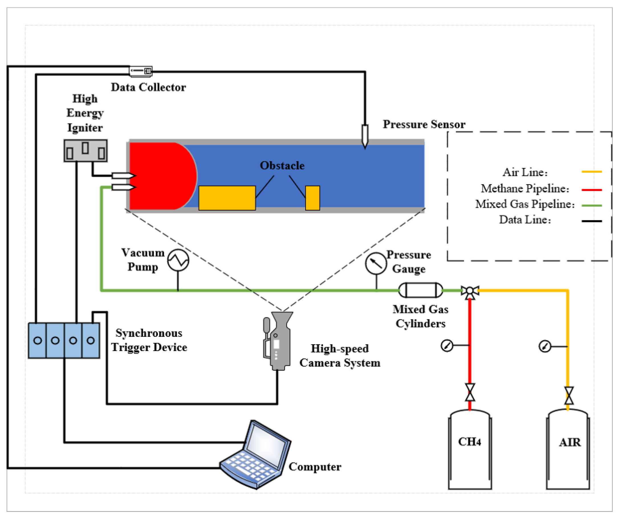
Figure 1. Experimental system.
Energies 17 04747 g001
Figure 2. Experimental equipment.
Energies 17 04747 g002
Figure 3. Flame diagram before and after grayscale.
Energies 17 04747 g003
Figure 4. GRU structure diagram.
Energies 17 04747 g004
Figure 5. Internal structure diagram of GRU neurons.
Energies 17 04747 g005
Figure 6. The structure of the proposed model.
Energies 17 04747 g006
Figure 7. Single obstacle peak flame velocity diagram: (a) Length 0.12 m. (b) Length 0.15 m.
Energies 17 04747 g007
Figure 8. The flame speed comparison diagram of rectangular obstacle with different ignition source distances.
Energies 17 04747 g008
Figure 9. The flame propagation velocity comparison diagram under different ignition source distance conditions with the same obstacle: (a) Length 0.12 m. (b) Length 0.15 m.
Energies 17 04747 g009
Figure 10. The flame speed comparison diagram of different shapes of obstacles with same ignition source distances.
Energies 17 04747 g010aEnergies 17 04747 g010b
Figure 11. Flame propagation velocity comparison diagram under same ignition source distance conditions with different shapes of the obstacle: (a) Length 0.12 m. (b) Length 0.15 m.
Energies 17 04747 g011
Figure 12. The peak flame velocity diagram for two obstacles condition: (a) Circular obstacle. (b) Rectangular obstacle. (c) Square obstacle.
Energies 17 04747 g012
Figure 13. The flame speed comparison diagram of different obstacle spacing with same obstacle shape and ignition source distances.
Energies 17 04747 g013
Figure 14. The flame propagation velocity comparison diagram under different distance between two obstacles condition.
Energies 17 04747 g014
Figure 15. The peak flame velocity diagram under conditions of the barbed wire obstacle and the circular obstacle.
Energies 17 04747 g015
Figure 16. The flame propagation velocity comparison diagram under conditions of the barbed wire obstacle and the circular obstacle.
Energies 17 04747 g016
Figure 17. The flame propagation velocity comparison diagram under conditions of coarse and fine barbed wire obstacles.
Energies 17 04747 g017
Figure 18. Comparison diagram of R2 mean value for different numbers of neurons in the neural network.
Energies 17 04747 g018
Figure 19. Comparison diagram of R2, MSE, and predicted values for different neural networks on the test set.
Energies 17 04747 g019
Figure 20. Comparison diagram of different neural networks prediction trends.
Energies 17 04747 g020
Figure 21. Comparison diagram of R2, MSE, and predicted values for different activation functions on the test set.
Energies 17 04747 g021
Figure 22. Comparison diagram of different activation functions prediction trends.
Energies 17 04747 g022
Figure 23. Comparison diagram of R2, MSE, and predicted values for different optimizers on the test set.
Energies 17 04747 g023
Figure 24. Comparison diagram of different optimizers prediction trends.
Energies 17 04747 g024
Figure 25. Prediction trends of flame propagation velocity by Zhang et al. [24].
Energies 17 04747 g025
Figure 26. Comparison diagram of R2 and MSE error bar after deleting a category of input vectors.
Energies 17 04747 g026
Table 1. Experimental conditions.
Experimental ConditionsNumber of ObstaclesObstacle ShapeObstacle Spacing
(m)
The Distance between the Obstacle and the Ignition Source (m)VBR
(10−2)
ABR
(10−2)
P/DPeak Flame Velocity (m/s)
11Circular obstacle with length of 0.12 m × radius of 0.0384 m00.052.76.9029.79
20.12.76.9035.47
30.152.76.9043.27
40.22.76.9053.91
50.252.76.9056.75
60.32.76.9056.04
70.352.76.9056.04
80.42.76.9053.2
90.452.76.9049.65
101Rectangular obstacle with length of 0.12 m × width of 0.06 m × height of 0.077 m00.052.77.6029.08
110.12.77.6031.92
120.152.77.6044.69
130.22.77.6051.78
140.252.77.6056.04
150.32.77.6053.91
160.352.77.6051.07
170.42.77.6049.65
180.452.77.6045.40
191Square
obstacle with length of 0.12 m × width of 0.068 m × height of 0.068 m
00.052.657.7031.21
200.12.657.7034.05
210.152.657.7042.56
220.22.657.7047.53
230.252.657.7051.07
240.32.657.7058.88
250.352.657.7049.65
260.42.657.7047.53
270.452.657.7043.98
281Circular obstacle with length of 0.15 m × radius of 0.0384 m00.053.318.3035.47
290.13.318.3040.43
300.153.318.3063.84
310.23.318.3053.91
320.253.318.3062.42
330.33.318.3053.91
340.353.318.3050.36
350.43.318.3049.65
360.453.318.3048.24
371Rectangular obstacle with length of 0.15 m × width of 0.06 m × height of 0.077 m00.053.319.2028.37
380.13.319.2030.50
390.153.319.2043.27
400.23.319.2046.82
410.253.319.2056.75
420.33.319.2048.94
430.353.319.2047.53
440.43.319.2046.82
450.453.319.2044.69
461Square
obstacle with length of 0.15 m × width of 0.068 m × height of 0.068 m
00.053.319.1028.37
470.13.319.1034.05
480.153.319.1041.85
490.23.319.1046.11
500.253.319.1049.65
510.33.319.1051.07
520.353.319.1046.82
530.43.319.1042.56
540.453.319.1041.14
552Circular obstacles with length of 0.12 m × radius of 0.0384 m;
length of 0.03 m ×
radius of 0.0384 m
0.080.053.39.91.052.49
560.13.39.91.063.13
570.153.39.91.060.29
580.23.39.91.058.88
592Circular obstacles with length of 0.12 m × radius of 0.0384 m;
length of 0.03 m ×
radius of 0.0384 m
0.160.053.39.92.162.42
600.13.39.92.168.81
610.153.39.92.166.68
620.23.39.92.164.55
632Circular obstacles with length of 0.12 m × radius of 0.0384 m;
length of 0.03 m ×
radius of 0.0384 m
0.240.053.39.93.156.75
640.13.39.93.156.75
650.153.39.93.161.71
660.23.39.93.161.00
672Rectangular obstacles with length of 0.12 m × width of 0.06 m × height of 0.077 m;
length of 0.03 m × width of 0.06 m × height of 0.077 m
0.080.053.310.81.247.53
680.13.310.81.253.20
690.153.310.81.261.71
700.23.310.81.259.58
712Rectangular obstacles with length of 0.12 m × width of 0.06 m × height of 0.077 m;
length of 0.03 m × width of 0.06 m × height of 0.077 m
0.160.053.310.82.463.84
720.13.310.82.467.39
730.153.310.82.465.26
740.23.310.82.463.13
752Rectangular obstacles with length of 0.12 m × width of 0.06 m × height of 0.077 m;
length of 0.03 m × width of 0.06 m × height of 0.077 m
0.240.053.310.83.655.33
760.13.310.83.661.00
770.153.310.83.658.88
780.23.310.83.661.00
792Square
obstacles with length of 0.12 m × width of 0.068 m × height of 0.068 m;
length of 0.03 m × width of 0.068 m × height of 0.068 m
0.080.053.310.71.246.11
800.13.310.71.258.88
810.153.310.71.261.00
820.23.310.71.253.91
832Square
obstacles with length of 0.12 m × width of 0.068 m × height of 0.068 m;
length of 0.03 m × width of 0.068 m × height of 0.068 m
0.160.053.310.72.456.75
840.13.310.72.465.26
850.153.310.72.461.71
860.23.310.72.454.62
872Square
obstacles with length of 0.12 m × width of 0.068 m × height of 0.068 m;
length of 0.03 m × width of 0.068 m × height of 0.068 m
0.240.053.310.73.549.65
880.13.310.73.551.78
890.153.310.73.556.75
900.23.310.73.553.20
911Thick barbed wire obstacle with Length 0.12 m × width 0.12 m × height 0.12 m× diameter 0.002 m00.050.056.6046.82
920.10.056.6063.97
930.150.056.6066.20
940.20.056.6065.97
950.250.056.6069.52
960.30.056.6065.97
970.350.056.6062.42
980.40.056.6061.00
990.450.056.6060.29
1001Thick barbed wire obstacle with Length 0.12 m × width 0.12 m × height 0.12 m × diameter 0.001 m00.050.024.3048.24
1010.10.024.3061.68
1020.150.024.3064.55
1030.20.024.3068.81
1040.250.024.3067.58
1050.30.024.3061.62
1060.350.024.3058.49
1070.40.024.3057.46
1080.450.024.3056.75
Table 2. Comparison table of R2 mean value for different numbers of neurons in the neural network.
Neural NetworkNumber of Neurons
48121620242832
RNN R2 mean value0.1270.1580.1950.2490.3530.4960.5030.508
LSTM R2 mean value0.3160.3580.3840.4250.4780.5240.5280.531
GRU R2 mean value0.3510.4610.5150.5590.5590.5790.5840.583
Table 3. Comparison table of R2 mean value for different neural networks.
Neural NetworkFlame Propagation Velocity
R2 Mean ValueDiscrete Range
RNN0.49630.0594
LSTM0.521510.09936
GRU0.561820.05034
Table 4. Comparison table of MSE mean value for different neural networks.
Neural NetworkFlame Propagation Velocity
MSE Mean ValueDiscrete Range
RNN94.1075411.09771
LSTM89.3986518.56359
GRU81.867539.40571
Table 5. Comparison table of R2 mean value for different activation functions.
Activation FunctionsFlame Propagation Velocity
R2 Mean ValueDiscrete Range
Sigmoid0.561820.05034
Relu0.827030.04411
PReLU0.866520.04793
Table 6. Comparison table of MSE values for different activation functions.
Activation FunctionsFlame Propagation Velocity
MSE Mean ValueDiscrete Range
Sigmoid81.867539.40571
Relu32.316618.24081
PReLU24.93948.95485
Table 7. Comparison table of test set R2 mean value for different optimizers.
OptimizersFlame Propagation Velocity
R2 Mean ValueDiscrete Range
Lookahead0.893020.05377
RAdam0.93630.02897
Adam0.942050.01712
Ranger0.961640.00462
Table 8. Comparison table of test set MSE mean value for different optimizers.
OptimizersFlame Propagation Velocity
MSE Mean ValueDiscrete Range
Lookahead19.9867710.04713
RAdam11.901855.41242
Adam10.827323.19952
Ranger7.167590.86213
Table 9. Comparison table of training and test set R2 mean value for Ranger optimizer.
DatasetFlame Propagation Velocity
R2 Mean ValueDiscrete Range
Training set0.971380.00572
Test set0.963050.00264
Table 10. Comparison table of training and test set MSE mean value for Ranger optimizer.
DatasetFlame Propagation Velocity
MSE Mean ValueDiscrete Range
Training set4.351440.85313
Test set6.269590.75461
Table 11. Prediction R2 and MSE mean value of flame propagation velocity by Zhang et al. [24].
Mean ValueFlame Propagation Velocity
R2 Mean ValueDiscrete Range
R20.962840.01705
MSE6.148961.57695
Table 12. Comparison table of R2 mean value after deleting a category of input vectors.
Category of Input VectorsFlame Propagation Velocity
R2 Mean ValueDiscrete Range
Obstacle shape0.674490.08546
Obstacle spacing0.681460.06181
P/D0.707520.04987
VBR0.682110.09198
ABR0.692950.09818
Distance between obstacle and ignition source0.695740.09034
Table 13. Comparison table of MSE mean value after deleting a category of input vectors.
Category of Input VectorsFlame Propagation Velocity
MSE Mean ValueDiscrete Range
Obstacle shape26.355823.33943
Obstacle spacing26.628412.41526
P/D27.646891.94863
VBR26.653553.59428
ABR27.077473.83643
Distance between obstacle and ignition source27.186393.53009
Disclaimer/Publisher’s Note: The statements, opinions and data contained in all publications are solely those of the individual author(s) and contributor(s) and not of MDPI and/or the editor(s). MDPI and/or the editor(s) disclaim responsibility for any injury to people or property resulting from any ideas, methods, instructions or products referred to in the content.