Enhancing Aggregate Load Forecasting Accuracy with Adversarial Graph Convolutional Imputation Network and Learnable Adjacency Matrix

Abstract

Accurate load forecasting, especially in the short term, is crucial for the safe and stable operation of power systems and their market participants. However, as modern power systems become increasingly complex, the challenges of short-term load forecasting are also intensifying. To address this challenge, data-driven deep learning techniques and load aggregation technologies have gradually been introduced into the field of load forecasting. However, data quality issues persist due to various factors such as sensor failures, unstable communication, and susceptibility to network attacks, leading to data gaps. Furthermore, in the domain of aggregated load forecasting, considering the potential interactions among aggregated loads can help market participants engage in cross-market transactions. However, aggregated loads often lack clear geographical locations, making it difficult to predefine graph structures. To address the issue of data quality, this study proposes a model named adversarial graph convolutional imputation network (AGCIN), combined with local and global correlations for imputation. To tackle the problem of the difficulty in predefining graph structures for aggregated loads, this study proposes a learnable adjacency matrix, which generates an adaptive adjacency matrix based on the relationships between different sequences without the need for geographical information. The experimental results demonstrate that the proposed imputation method outperforms other imputation methods in scenarios with random and continuous missing data. Additionally, the prediction accuracy of the proposed method exceeds that of several baseline methods, affirming the effectiveness of our approach in imputation and prediction, ultimately enhancing the accuracy of aggregated load forecasting.

1. Introduction

Electric load forecasting, especially short-term electric load forecasting, holds paramount importance for the optimization of the power system′s operations and its significance to participants in the electricity market. Accurate electric load forecasts serve as valuable tools in assisting power system operation planning, electricity price structuring, and energy transactions, thereby enhancing the system’s efficiency and economic benefits [1,2]. However, the rapid proliferation of distributed energy sources, electric vehicles, and demand response introduces a growing level of uncertainty into load forecasting, making precise short-term load predictions an increasingly formidable endeavor [3].

In contrast to traditional statistical forecasting methods, artificial intelligence techniques exhibit enhanced nonlinear fitting capabilities and superior generalization, thereby facilitating the acquisition of more precise forecasting results. The application of deep learning in load forecasting dates back to the 1990s [4,5,6]. Currently, prevalent deep learning models employed in load forecasting predominantly encompass long short-term memory (LSTM) [7,8], temporal convolutional network (TCN) [9,10,11], and their counterparts. These methodologies predominantly emphasize temporal correlations within user load sequences, often neglecting the latent connections among individual users. Nevertheless, users residing in geographically proximate locations experience similar influences from weather conditions and holiday patterns. Similarly, users situated in non-adjacent geographic locations might exhibit analogous load patterns due to shared electrical equipment or consumption habits. Thus, it is imperative to consider the interrelations among users in load forecasting.

In load forecasting, the methods that consider the relationships between users mainly include those based on convolutional neural network (CNN) [12,13], graph convolutional networks (GCNs) [14,15,16,17], and Transformer [18,19]. CNN-based methods are adept at capturing spatial correlations within regular Euclidean spaces, making them useful for extracting features from grid-like, spatially distributed user data. However, they might fall short when it comes to capturing complex relationships between users that do not conform to such regular, structured grids. This limitation makes CNN less suitable for describing the intricate interconnections among users that often occur in non-Euclidean spaces. In contrast, GCNs are specifically designed to operate on graph-structured data, where relationships between users can be more irregular and complex. GCN excel at extracting both node-specific information and the latent connections among users in these non-Euclidean spaces, thereby enhancing forecasting accuracy by considering the interdependencies between geographically or behaviorally similar users. Transformers, initially introduced for natural language processing tasks, have also shown promise in load forecasting. Transformers are particularly strong when it comes to capturing long-range dependencies within data, making them well suited for forecasting tasks that require an understanding of both temporal sequences and the underlying relationships between users. However, their global self-attention mechanism, while powerful, can lead to unnecessary computational complexity and efficiency issues in short-term forecasting tasks, especially in scenarios where spatial relationships change frequently. This characteristic may make Transformers less efficient compared to other models when dealing with rapidly changing or localized data, where the complexity of the attention mechanism does not necessarily translate to a better predictive performance [20].

Table 1. Summary of load forecasting methods.

Model	Advantages	Disadvantages
LSTM-based [7,8]	Mature theory and well suited for time series data; effective at capturing long-term dependencies in sequences.	Computationally expensive, especially for long sequences; susceptible to vanishing gradient problems with very long sequences; cannot model correlation between users.
TCN-based [9,10,11]	Supports parallel computing, improving efficiency; can model long-term dependencies with dilated convolutions.	May require careful tuning of dilation factors and convolutional filters; potentially high memory usage due to large filter sizes; cannot model correlation between users.
CNN-based [12,13]	Efficient at capturing spatial correlations in structured data; can be used with regular grid-like structures in Euclidean spaces.	Less effective for irregular, non-Euclidean relationships among users; lacks the ability to capture temporal dependencies directly.
GCN-based [14,15,16,17]	Excels at modeling complex relationships in graph-structured data; effectively captures both local and global relationships in non-Euclidean spaces.	Requires predefined or learned adjacency matrices, which may not always be straightforward; computational complexity can be high for large graphs.
Transformer-based [18,19]	Good at capturing long-range dependencies within data; flexible attention mechanisms that can adapt to various tasks.	Global attention mechanism can add unnecessary complexity in short-term tasks; sufficient computing resources and datasets are required.

summarizes the current load forecasting methods.

Aggregate load refers to the integration of the loads from multiple users or devices into a unified energy load, facilitating centralized control and management. In contrast to load forecasts at the user level, aggregate load forecasts exhibit reduced uncertainty due to the amalgamation of diverse user load behaviors. The collective behaviors of numerous users often offset each other’s uncertainties relatively smoothly, thereby resulting in higher forecast precision [21]. Aggregate load forecasting holds paramount significance in demand response [22,23], power system planning [24], and the development of electricity markets [25]. Moreover, within cross-market transactions, the consideration of correlations among multiple aggregate loads assists market participants in understanding load correlations between different markets, facilitating a better balance of load demands and the formulation of suitable trading strategies.

Considering the limitations of CNNs, which are adept at capturing spatial correlations within regular Euclidean spaces but struggle with irregular and non-Euclidean relationships among loads, and the potential inefficiencies of Transformers, which may introduce unnecessary computational complexity in short-term forecasting tasks due to their global self-attention mechanisms, this paper proposes the application of deep learning to aggregate load forecasting by employing a GCN. The GCN is utilized to explore and leverage the correlations among aggregate loads, thereby enhancing predictive accuracy. However, we confront two primary challenges:

Data quality: Deep learning is a data-driven model, and high-quality data are indispensable for precise load forecasting. Issues such as sensor malfunctions, communication instability, and susceptibility to network attacks can compromise data quality, leading to incomplete load data.

Adjacency matrix: In the utilization of GCN for user load prediction, relationships among users are represented as a graph structure through the adjacency matrix. Currently, a prevalent approach constructs the adjacency matrix based on the geographic distance between users, necessitating the predefinition of the graph structure [26]. However, for entities like aggregate loads that lack distinct spatial geographic positions, the usage of distance-based methods to construct an adjacency matrix is impractical. Consequently, an approach is required that can derive an adjacency matrix without the need for predefining the graph structure.

Regarding issue 1, the current approaches for handling missing data can be categorized into direct deletion and imputation methods. Direct deletion, while simple, is suitable only for cases where the proportion of missing values is small. When missing values are prevalent, this method leads to a loss of crucial information, resulting in poor model performance or even training failure. Imputation methods can be divided into two categories. The first category is based on inferring missing values from similar data points, including methods such as using simple statistics (e.g., mean, median) [27] and K-nearest neighbors (KNN) [28]. The second category involves establishing a global model based on the entire dataset for imputation, including multiple imputation and generative adversarial networks (GANs). Refs. [29,30] employ a KNN-based imputation method, which is straightforward but is limited to modeling similarities between data points, lacking the construction of a global model and resulting in lower imputation accuracy. Ref. [31] introduces a multiple imputation by chained equations (MICE) method, which iteratively traverses the entire dataset to obtain data association rules and utilizes these rules for imputation, making it a popular imputation method. Deep learning, with its multi-layered nonlinear structures, offers advantages in capturing complex data correlations and building global models. GANs, as a class of deep learning generative models, are capable of generating samples similar to the original data and adhering to the same probability distribution, thus improving data quality when the original dataset is of low quality [32]. Refs. [33,34,35] utilize GANs for the reconstruction of missing data in power system measurements, achieving favorable results. While methods based on similar data points are straightforward, they are limited by local similarity and lack global dataset information. On the other hand, methods based on global models can utilize features and distribution information from the entire dataset but come with higher computational complexity and sensitivity to extreme data points. As a result, this paper proposes an imputation method that simultaneously considers both local and global aspects. It initially uses a GCN to uncover potential connections between similar data points, constructing a local imputation model. Then, it employs a GAN to build a global imputation model. The combination of these two approaches enhances imputation accuracy [36].

Table 2. Summary of imputation methods.

Model	Advantages	Disadvantages
Mean, median [27]	Simple and easy to implement; high computational efficiency.	Focus only on local features; assumes a simple underlying distribution; limited in handling complex data patterns.
KNN [28,29,30]	Captures local similarities effectively; non-parametric method; flexible and easy to interpret.	Requires careful tuning of neighbors; does not model global dependencies; less effective for larger datasets.
MICE [31]	Handles multiple imputations; effective for capturing data associations; suitable for handling missing data across multiple variables.	Strong assumptions about missing patterns; struggles with temporal dependencies.
GAN-based [32,33,34,35]	Capable of generating realistic data; robust against missing data; captures global dependencies; handles complex data structures.	Limited attention to local features; high computational cost; requires large datasets; needs careful tuning to avoid mode collapse; complex to implement and train.

summarizes the current imputation methods.

Regarding issue 2, the current methods for constructing adjacency matrices for users without explicit geographical locations primarily include correlation coefficient-based adjacency matrices and binary adjacency matrices. Both of these methods calculate the adjacency matrix by computing the correlation coefficients between different user load sequences. The latter, a binary adjacency matrix, is derived from the correlation coefficient matrix by applying a threshold. The advantages of these two adjacency matrix construction methods lie in their simplicity and computational efficiency. However, their drawback is that correlation coefficients can only reflect linear relationships between user sequences and cannot capture complex nonlinear relationships. Therefore, this paper proposes a learnable adjacency matrix, which can adaptively learn the interrelationships between different sequences to obtain the adjacency matrix. Compared to correlation coefficients, this approach can better capture the intricate relationships between user sequences. It can automatically adjust the strength of connections based on the data’s characteristics, thus accommodating different data distributions and features. This method proves effective for obtaining the adjacency matrix when the graph structure cannot be predefined.

Hence, in response to the issues outlined in the realm of user load forecasting, this paper’s contributions can be summarized as follows:

(1) We introduce an adversarial training-based graph convolutional imputation neural network that simultaneously considers both local and global correlations during the imputation process, aiming to enhance imputation accuracy. This involves the initial establishment of a local imputation model using GCN autoencoders, followed by the construction of a global imputation model through GAN-based adversarial training. Empirical evidence has solidly confirmed the effectiveness of this imputation model.

(2) We propose a method for the adaptive construction of an adjacency matrix through active learning of inter-sequence correlations. This method effectively addresses the limitations of traditional approaches, which lack flexibility and depend on spatial information, as demonstrated through empirical validation. The result is an improvement in prediction accuracy.

The remainder of the paper is organized as follows. In Section 2, the framework for load imputation and prediction is introduced. In Section 3, the experiments are introduced. In Section 4, extended experiments on a public dataset are conducted. Finally, Section 5 provides the conclusions.

2. Materials and Methods

2.1. Load Imputation Framework

In this section, we will elucidate the framework of the missing data imputation model AGCIN. The AGCIN model simultaneously considers both local and global correlations to enhance imputation accuracy. The model consists of two components:

Local imputation model (GCN-based): This component utilizes GCN to explore the relationships between similar data points. It makes preliminary inferences on missing values based on the connections between nodes and information from neighboring nodes, thereby constructing a local imputation model. During this phase, the model primarily focuses on the local relationships between nodes, filling in missing values while preserving local continuity in the data.

Global imputation model (GAN-based): Building upon the local imputation model, this component introduces GAN for adversarial training. GCN acts as the generator, providing feedback during the adversarial training process to enhance imputation effectiveness. It further refines and infers the results of local imputation. This process aims to make the overall probability distribution of the imputed data closely resemble the true probability distribution, thus constructing a global imputation model. In the global imputation phase, the model shifts its focus from local relationships to the distribution characteristics of the entire dataset, ensuring global consistency while filling in missing values.

The relationship between these two components is depicted in Figure 1. The local imputation stage emphasizes relationships between nodes and their neighbors to fill in missing values while maintaining local continuity. In the global imputation stage, the model concentrates on the distribution characteristics of the entire dataset to preserve global consistency while imputing missing values.

2.1.1. Local Imputation Model

In mathematics, a graph serves as a mathematical concept that is utilized to elucidate the structural connections amid a set of entities. These entities typically correspond to the nodes (or vertices) within the graph, while the interrelations between these nodes find representation through an adjacency matrix. Ordinarily, a graph’s delineation encompasses the ensuing elements [15]:

$$G=(V,E,A)$$

(1)

where G represents the graph, V stands for the nodes (or vertices) of the graph, E represents the edges of the graph, and A signifies the adjacency matrix of the graph.

Graph convolution stands as a pivotal technique for handling unstructured data, facilitating the extraction of features from graphs. In the realm of graph convolution, the graph’s Laplacian matrix is defined as L = D − A, where D represents the graph’s diagonal matrix and A is the adjacency matrix of the graph. Accordingly, the expression for graph convolution, as per Ref. [37], is articulated as follows:

$$y=\sigma (\tilde{L}X\theta )$$

(2)

where $\tilde{L}$ denotes the symmetrically normalized Laplacian matrix and $\theta$ represents an adaptive coefficient matrix. The left multiplication allows information to propagate between adjacent nodes. The right multiplication acts akin to a fully connected layer, amalgamating the features extracted earlier. A GCN is composed of multiple stacked graph convolutional layers.

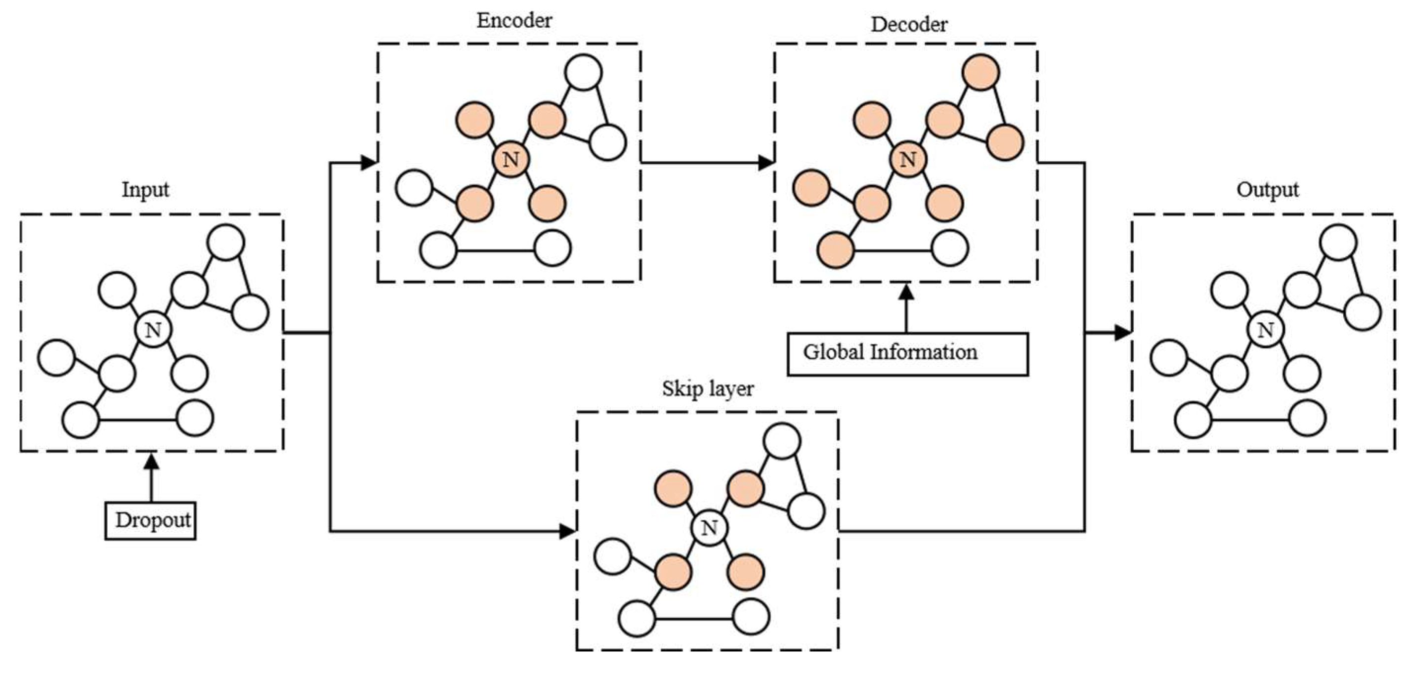
Constructing a local imputation model using GCN involves the transformation of raw data into graph-structured data. Each feature vector in the raw dataset is represented as a node in the graph. Subsequently, the similarities between nodes are calculated to form a similarity matrix. This matrix is then processed to obtain the adjacency matrix, from which the graph-structured data can be derived. In this paper, the Euclidean distance is employed to construct a similarity matrix for all feature vectors, with calculations performed on pairs of vectors at a time. Furthermore, due to the presence of missing data in the dataset, a binary mask matrix M is introduced to indicate data completeness. When M = 0, it signifies an absence of data; when M = 1, it indicates data completeness. Figure 2 shows the structure of the local imputation model.

The similarity calculation formula based on Euclidean distance is as follows [38]:

$$S_{ij}=d(x_i\odot (M_i\odot M_j),x_j\odot (M_i\odot M_j))$$

(3)

where $d$ represents the Euclidean distance, $\odot$ signifies the Hadamard product (element-wise multiplication), and $M_i$ represents the ith column of the matrix.

The similarity matrix obtained from this process is a dense matrix, which comes with a high computational cost and can be challenging to directly apply in graph convolution. It requires a threshold truncation operation to obtain a sparse matrix. In this paper, each row of the similarity matrix is sorted in descending order, and a percentile p is specified. Only the top p% of values in each row are retained. This is represented by the following formula [39]:

$$A_{ij}=\left\{\begin{array}{cc}{S}_{ij},\hfill & if S_{ij}\ge To{p}_{p\%}(S_{i,:})\hfill \\ 0,\hfill & otherwise\hfill \end{array}\right.$$

(4)

After the completion of the process described in Equation (4), the resulting similarity matrix $S_{ij}$ serves as the adjacency matrix $A_{ij}$ for AGCIN. Through threshold truncation, GCN retains only the connections above the threshold and prunes the rest. This results in a sparsely connected graph, greatly reducing computational costs. Furthermore, pruning discards less relevant information while retaining more valuable data. Upon transforming the raw data into a graph structure, a local imputation model is constructed using a GCN autoencoder. Information propagation occurs through non-missing data and the relationships between nodes to estimate the missing values. The autoencoder comprises an encoder and a decoder. The encoder maps the original input x into a lower-dimensional space $h=encode(x)$ for intermediate representation, while the decoder maps the encoded input back into the original dimension to reconstruct the input: $\widehat{x}=decode(h)$. Through training, the goal is to minimize the error between $x$ and the reconstructed data $\widehat{x}$, enhancing the accuracy of reconstruction. In the encoding phase, the graph convolution involves only 1st-order neighboring nodes. However, in the decoding phase, to acquire more neighbor node information and improve reconstruction accuracy, the graph convolution extends to 2nd-order neighboring nodes. Additionally, to enhance data imputation quality, a skip layer and global information are incorporated into the decoder. The graph convolution operation performed in the skip layer is akin to that in the encoder, with the key difference being that the graph convolution in the skip layer excludes the node itself. Consequently, the skip layer’s output comprises information from neighboring nodes only, excluding information from the current node. This encourages the model to learn similarity between adjacent nodes, preventing the autoencoder from learning an identity function and thus enhancing the model’s understanding and ability to reconstruct the data. To increase the contribution of the most similar nodes, the skip layer only considers 1st-order neighboring nodes. Given that GCN typically focuses on node and edge-level information, the addition of global information enhances the expressiveness of the graph neural network. Global information usually refers to statistical information for the entire dataset, such as averages and modes. In this paper, the average is used as global information, and a global information vector g is introduced in the decoder. This global information is combined with each node through weighted aggregation, reinforcing the expressive power of node representations [40].

In accordance with the definition of graph convolution provided in Equation (2), the encoder and decoder in AGCIN can be defined as follows [36]:

$$H=\mathrm{Re}lu(\tilde{L}X{\theta }_1)$$

(5)

$$\widehat{X}=Sigmoid(\tilde{L}X{\theta }_2+{\tilde{L}}^{\prime }X{\theta }_3+{\theta }_{4}g)$$

(6)

where ${\tilde{L}}^{\prime }$ represents the symmetrically normalized Laplacian matrix, excluding self-connections, and g is the global information vector, which is integrated with each node through weighted aggregation.

However, due to the presence of missing data, which is unknown during the training phase and cannot be directly used to train the autoencoder, a denoising autoencoder (DAE) [41] is employed. A denoising autoencoder takes noisy original samples (corrupted original samples) as input and reconstructs the original samples as output. In this paper, dropout layers are used to randomly remove 50% of the input, which is then used as input to the DAE to reconstruct the original input.

The mean squared error (MSE) is utilized as the loss function for the autoencoder in this paper:

$$L_1=MSE(X,\widehat{X})$$

(7)

2.1.2. Global Imputation Model

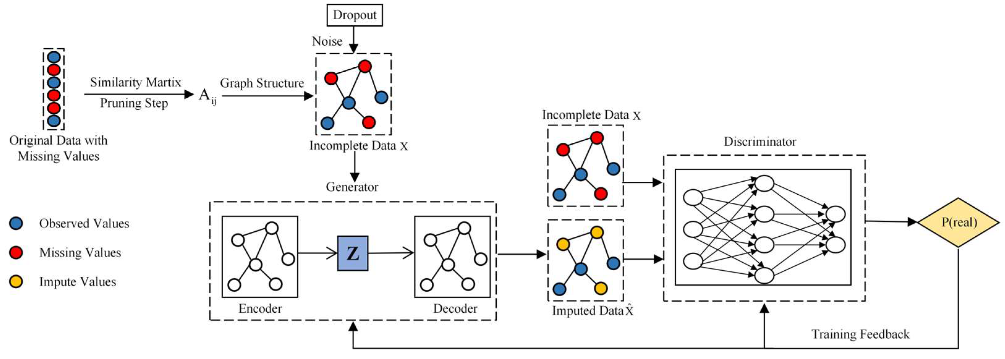
Due to the excellent performance of GAN in data reconstruction, this paper considers introducing adversarial training on top of using GCN to uncover latent correlations between data. This forms the foundation of the global imputation AGCIN model. GAN consists of a generator and a discriminator. The generator is responsible for creating counterfeit data, while the discriminator is responsible for distinguishing between the generated counterfeit data and real data. They engage in adversarial training, ultimately forcing the probability distribution of the generated counterfeit data to closely match the probability distribution of real data. In the AGCIN model, the generator employs a GCN-based autoencoder, while the discriminator uses a multi-layer perceptron (MLP). The structure of the AGCIN model is illustrated in Figure 3. Initially, the model performs local imputation through the generator to obtain filled data. Then, it feeds both the original data $X$ and the filled data $\widehat{X}$ into the discriminator. The discriminator outputs the probability of their authenticity. The discriminator and generator update through training feedback. After multiple rounds of adversarial training, the filled data $\widehat{X}$ closely approximate the probability distribution of the real incomplete data $X$. Finally, the corresponding values are used to complete the missing parts of $X$, achieving global imputation of the data. Traditional GAN in training suffer from mode collapse and gradient vanishing problems. Scholars later proposed using Wasserstein distance, known as WGAN (Wasserstein GAN), to address these issues. However, WGAN employs weight clipping to constrain the discriminator’s network parameters, which can lead to uneven parameter value distributions and unstable training. WGAN-GP (Wasserstein GAN with gradient penalty), built upon WGAN, introduced gradient penalty as an alternative to weight clipping, improving training stability and making it easier to generate high-quality samples [35]. Therefore, the GAN model adopted in this paper is in the form of WGAN-GP. The loss function employed in this paper for WGAN-GP is [42]:

$$L_2=-E_{x\sim p(x)}[D(X)]+E_{\widehat{x}\sim p(\widehat{x})}[D(\widehat{X})]+\lambda E{[‖\nabla {D(X^{\prime })‖}_2-1]}^2$$

(8)

where $E(\cdot )$ represents the mathematical expectation and $p(x)$ and $p(\widehat{x})$ are the probability distributions of real data x and generated data, respectively. $D(\cdot )$ is the discriminator’s function and $\lambda$ is the weight coefficient for the gradient penalty term, where $X^{\prime }=\epsilon X+(1-\epsilon )\widehat{X}$, $\epsilon$ is a random number.

Furthermore, in order to improve the generator’s ability to deceive the discriminator while minimizing reconstruction error, the generator’s loss function needs to be modified as follows [36]:

$$L_3=L_1-E_{\widehat{x}\sim p(\widehat{x})}[D(\widehat{X})]$$

(9)

During the training process, the discriminator’s weights are updated five times, while the generator is updated once. The primary purpose of training the discriminator more frequently is to enable it to more accurately distinguish between generated data and real data. This also helps prevent excessive training of the generator, which could introduce more noise into the process, thereby stabilizing the training process and improving the quality of generated data.

2.2. Load Forecasting Framework

2.2.1. Spatio-Temporal Correlation

Different users’ electricity consumption behaviors are not completely independent; they are interconnected and mutually influencing. Therefore, there is a certain spatial influence among different users’ loads. Time-series-based forecasting methods cannot reflect this spatial correlation. Hence, there is a need for spatio-temporal load forecasting, considering both the time-related and spatial-related aspects of user loads to further enhance prediction accuracy.

Spatio-temporal load forecasting is fundamentally a multivariate time series forecasting problem. Let $[{\mathrm{X}}_1^t\cdots {\mathrm{X}}_N^t]\in R^{N\times D}$ represents a collection of D features for N users at a given moment in time, ${\mathrm{x}}_i^t=[x_i^{t,1}\cdots x_i^{t,D}]\in R^D$ represents the D feature sets of the ith user at time t, $[{\mathrm{X}}^1\cdots {\mathrm{X}}^T]\in R^{T_{in}\times N\times D}$ represents the D feature sets of N users at T time steps, and $[{\mathrm{Y}}^{T+1}\cdots {\mathrm{Y}}^{T+Q}]\in R^{T_{out}\times N}$ represents the collection of predicted load values for N users in the future Q time steps. Therefore, utilizing LASTGCN for load forecasting can be expressed as follows:

$$\{{\mathrm{X}}^1{,\mathrm{X}}^2,\cdots {\mathrm{X}}^T,\mathrm{G}\}\stackrel{f(·)}{\to }\{{\mathrm{Y}}^{T+1}{,\mathrm{Y}}^{T+2},\cdots {\mathrm{Y}}^{T+Q}\}$$

(10)

where the left side is the historical information of N users for T time steps; G represents the graph structure information, including nodes and edges; $f(·)$ denotes the prediction function; on the right side is the future information of N users for Q time steps.

The LASTGCN model advances load forecasting by integrating dynamic spatial and temporal dependencies, overcoming the limitations of traditional models. It consists of a learning layer, mix-hop graph convolutional layers, TCN layers, and a 1 × 1 standard convolutional layer. The 1 × 1 standard convolutional layer projects inputs into a latent space for deeper learning and processing. The learning layer generates a learnable adjacency matrix, adapting to changing spatial relationships by capturing interactions between users and converting them into graph-structured data. This matrix, which is used as input for the graph convolutional layers, enhances the model’s ability to capture spatial correlations, such as load propagation and regional influences. The TCN layers further capture time dependencies and periodicities, revealing patterns and trends in the time series. Unlike CNNs with fixed spatial data and static kernels, LASTGCN’s adaptive matrix dynamically adjusts to evolving dynamics, improving the prediction accuracy in dynamic power systems. The model structure is illustrated in Figure 4.

Additionally, LASTGCN avoids the computational inefficiencies of Transformer models in short-term scenarios by focusing on local dependencies, optimizing computational resources. Furthermore, LASTGCN learns spatial relationships directly from data sequences without requiring predefined graph structures or external geographical information, making it robust and versatile, even in environments with sparse or incomplete data. To enhance training speed, the model incorporates residual and skip connections, ensuring efficient and accurate forecasting.

In the LASTGCN model, the loss function utilizes L2 regularization with the mean absolute error (MAE), as shown in the following formula [43]:

$$L={\displaystyle \frac{1}{n}}{\displaystyle {\sum }_{i=1}^n\left|y_i-{\widehat{y}}_i\right|}+{\displaystyle \frac{\lambda }{2n}}{{\displaystyle {\sum }_{i=1}^n\left|w_i\right|}}^2$$

(11)

where $n$ represents the number of samples; $y_i$ is the actual value and ${\widehat{y}}_i$ is the predicted value; $w_i$ represents the weight parameters; $\lambda$ is a hyperparameter used to control the regularization strength.

2.2.2. Learnable Adjacency Matrix

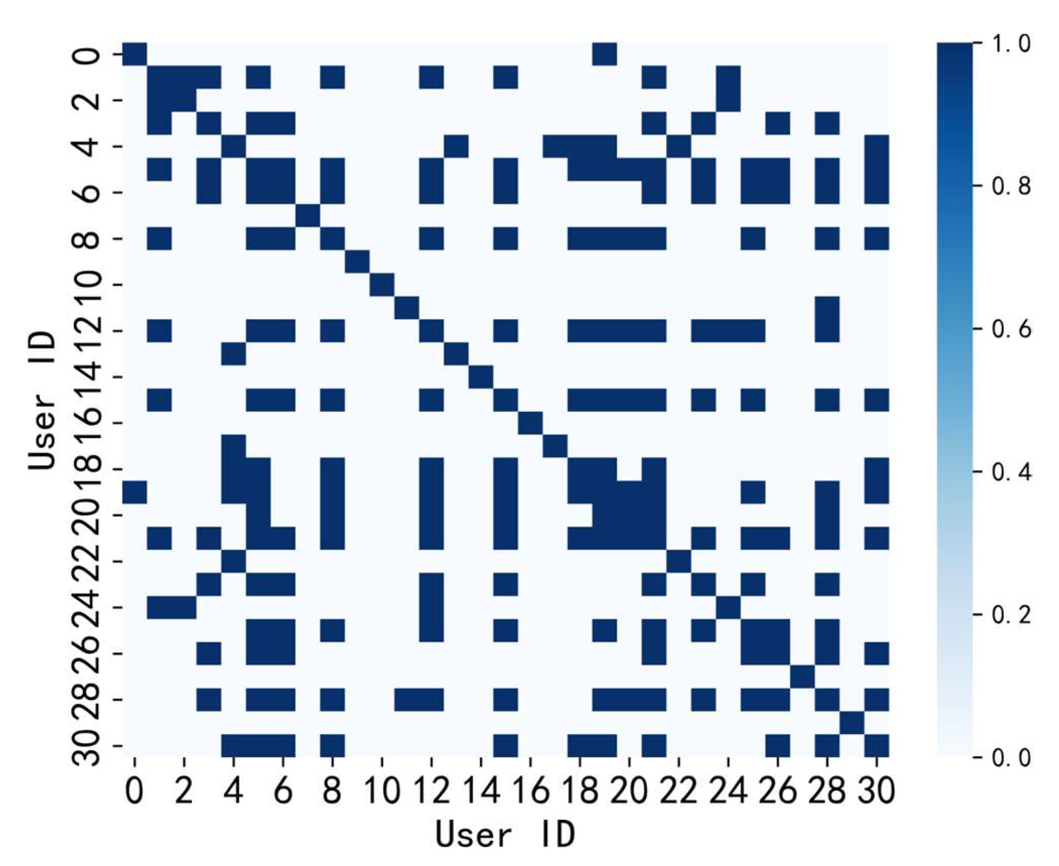
When using spatio-temporal GCN for load forecasting, it is common to process the geographical distances between users and use them as an adjacency matrix. However, this method requires defining the graph structure in advance, which is feasible when each user has a clear geographical location. But if there are users in the group, such as load aggregators, who do not have clear geographical locations, then this method cannot be used because the graph structure is not known in advance. Additionally, most adjacency matrices based on distance metrics are symmetric, which means that the strength of mutual influence between nodes is assumed to be equal. However, in reality, the strength of interactions between nodes can vary. Using an asymmetric adjacency matrix can more accurately describe the actual influence relationships between nodes, thus improving prediction accuracy. Therefore, this paper proposes a learnable asymmetric adjacency matrix for load forecasting. This method adapts by learning an adjacency matrix from the data to capture hidden relationships between time series data. The advantages of using a learnable adjacency matrix are as follows:

Adaptability: The matrix can adapt to different data distributions and relationships, making it versatile for various scenarios. Should a predefined graph structure undergo alterations, one would necessitate the manual updating of the adjacency matrix. However, with the utilization of a trainable adjacency matrix, the model can autonomously adapt the adjacency matrix based on shifts in the data, thereby accommodating distinct graph structures.

Improved accuracy: The matrix can capture complex and varying relationships between data points, which can lead to improved forecasting accuracy. Predefining a graph structure is often based on empirical or prior knowledge, whereas a trainable adjacency matrix is acquired through learning. This enables the model to autonomously glean relationships between nodes from the data, thereby making it capable of capturing more intricate interconnections among nodes.

In summary, the use of a learnable asymmetric adjacency matrix enhances the capabilities of spatio-temporal GCN for load forecasting by adapting to data-specific relationships and improving accuracy, even in scenarios with users who lack clear geographical locations.

The expression of the trainable adjacency matrix is as shown in the following equation [43]:

$$S_1=\tanh (\alpha E_1{\theta }_1)$$

(12)

$$S_2=\tanh (\alpha E_2{\theta }_2)$$

(13)

$$A_{asym}=\mathrm{ReLU}(\tanh \alpha (S_1{S}_2^T-S_2{S}_1^T))$$

(14)

where $E_1$ and $E_2$ represent randomly initialized node embeddings, which can be viewed as encoding representations of the original data and are updatable during the training process. ${\theta }_1$ and ${\theta }_2$ are model parameters. $\tan \mathrm{h}$ and $\mathrm{ReLu}$ denote activation functions, with $\mathsf{\alpha }$ serving as a hyperparameter that regulates the activation function’s saturation rate. $S_1$ and $S_2$, respectively, depict the results of nonlinear transformations applied to node embeddings, aiding in capturing intricate relationships between nodes. $A_{asym}$ signifies the learnable asymmetric adjacency matrix. It is derived by computing the difference matrix between $S_1,S_2$, and their transposes, followed by a nonlinear transformation. This process encompasses element-wise filtering of the adjacency matrix, strengthening connections between similar nodes and weakening connections between dissimilar nodes.

2.2.3. Spatial Feature Extraction

In the context of user load prediction, the purpose of graph convolution is to extract and aggregate the features of the target node with the features of its neighbors to handle spatial dependencies within the graph. In LASTGCN, each user is represented as a node in the graph, and to gather information from higher-order neighbors in the graph and improve prediction accuracy, a mix-hop propagation strategy is employed, as illustrated in Figure 5. Mix-hop is an enhanced form of graph convolution that can comprehensively capture the neighbor information of nodes compared to regular graph convolutions while also being computationally efficient, thereby enhancing feature representation capabilities. Specifically, the mix-hop strategy consists of two parts: information propagation and information selection. The expression for information propagation is as follows [44]:

$$H^{(k)}=\beta H_{in}+(1-\beta )A_{asym}{H}^{(k-1)}$$

(15)

where $k$ represents the propagation depth, indicating the number of neighbors considered at each level. $H^{\left(k\right)}$ denotes the hidden layer state of the k-th layer, while $H_{in}$ represents the current layer’s input hidden layer state, which corresponds to the output hidden layer state from the previous layer. $\beta$ is a hyperparameter that signifies the proportion of the original node information retained.

The expression for information selection is as follows [45]:

$$H_{out}={\displaystyle \sum _{i=0}^K{H}^{(k)}{W}^{(k)}}$$

(16)

where $W^{\left(k\right)}$ is a weight matrix utilized to select information from different neighboring nodes, which is updated during the training process, and $H_{out}$ represents the hidden layer state after information selection.

The graph convolution layer that utilizes the mix-hop propagation strategy is illustrated in Figure 6.

In Figure 6, the graph convolutional layer employs two mix-hop propagation layers, corresponding to the in-degree and out-degree information, respectively. This is because the adjacency matrix is asymmetric and using both in-degree and out-degree information helps capture a more comprehensive view of a node’s neighboring nodes, thereby enhancing the network’s expressive power.

2.2.4. Temporal Feature Extraction

Graph convolution itself primarily focuses on spatial relationships and does not inherently account for temporal dependencies. Therefore, incorporating TCN is a valuable addition to consider temporal relationships.

Compared to recurrent neural networks like recurrent neural network (RNN) and LSTM, which are used for time series modeling, TCN offers the advantage of parallel computation, resulting in higher computational efficiency. Additionally, TCN can alleviate issues such as gradient vanishing and exploding gradients that are often encountered in recurrent neural networks.

Within TCN, causal convolution is employed, ensuring that only past data are used to predict future data points. Future data points do not influence the predictions for the current time step, aligning with temporal constraints. To capture longer-term dependencies, dilated convolution is introduced in TCN, allowing for a larger receptive field with fewer network layers.

Furthermore, to enable TCN to capture periodic information of varying lengths within the time series and enhance the model’s understanding of sequences, this paper incorporates an inception module. Inception is a convolutional neural network architecture that leverages multiple convolutional kernels of different sizes in parallel to extract features from various scales simultaneously, thereby improving both the model’s performance and its computational efficiency [44]. The TCN with the addition of the inception module is expressed as follows [46]:

$$O=concat(Conv(X,K_{1\times 3},d=1),Conv(X,K_{1\times 6},d=2), Conv(X,K_{1\times 7},d=4))$$

(17)

$$Conv(X,K,d)={\displaystyle \sum _{s=0}^{K-1}{f}_{1\times k}}(s)X(t-ds)$$

(18)

where $Conv(X,K,d)$ represents the dilated convolution operation on input $X$ using a convolutional kernel K with a dilation factor of d, $f$ denotes the convolutional kernel function, and s indicates the convolutional kernel index. $concat$ denotes the concatenation of the three convolution results along the channel dimension. For instance, in the structure shown in Equation (17), convolutional kernels of sizes 1 × 3, 1 × 6, and 1 × 7 are employed with dilation factors of 1, 2, and 4, respectively. The convolution results combine information from different temporal lengths, enhancing the model’s expressive capacity.

3. Case Study

3.1. Data Source and Experimental Settings

The dataset employed in this paper comprises aggregate load data from Guangdong province, China, encompassing a total of 31 aggregate loads. These loads have been aggregated based on spatial location, with each aggregate load encompassing multiple user loads. The temporal scope of the dataset spans from 1 December 2020 to 31 March 2022 and includes solely historical load features, with a data resolution of 1 h. For both the imputation and prediction experiments, the data have been partitioned into training, validation, and test sets in a ratio of 7:1:2. Specifically, the training set covers the period from 1 December 2020 to 6 November 2021, the validation set spans from 7 November 2021 to 24 December 2021, and the test set includes data from 25 December 2021 to 31 March 2022. This partitioning approach ensures that the training set encompasses nearly a full year of data, covering different seasons, which allows the model to learn the distinct load patterns of each season. As a result, this comprehensive training enhances the model’s ability to generalize, leading to improved performance on the test set.

In addition, the dataset underwent several preprocessing steps to ensure its suitability for both imputation and forecasting tasks. For forecasting, the dataset did not contain any missing values, as the presence of missing data points would have hindered the evaluation of the imputation performance. However, for the imputation experiments, artificial missing values were intentionally introduced to the dataset to assess the effectiveness of the proposed imputation methods. Additionally, before feeding the data into the model, Min-Max normalization was applied to scale the features to a range between 0 and 1. This normalization step was crucial for enhancing the performance of the deep learning models. After the prediction process, the data were de-normalized to facilitate the calculation of performance metrics and for better visualization.

This experiment was conducted using the PyTorch 1.7.0 deep learning platform on a hardware platform consisting of Windows 10, a 64-bit operating system, an Intel Core i5-12400F CPU with a clock speed of 2.5 GHz, an NVIDIA GeForce RTX 3060 GPU, and 16 GB of memory.

3.2. Evaluation Metrics

In this experiment, the evaluation metrics used for assessing the experimental results are mean absolute error (MAE), root mean squared error (RMSE), and R-squared (R²) score. MAE and RMSE are employed to gauge the proximity between predicted values and actual values, where smaller values indicate a better prediction performance. The R² score measures the linear correlation between predicted values and actual values, with values closer to one indicating a stronger correlation and thus better prediction performance. The formulas are as follows:

$$\mathrm{MAE}={\displaystyle \frac{1}{n}}{\displaystyle {\sum }_{i=1}^n\left|y_i-{\widehat{y}}_i\right|}$$

(19)

$$\mathrm{RMSE}=\sqrt{{\displaystyle \frac{1}{n}}{\displaystyle {\sum }_{i=1}^n{\left|y_i-{\widehat{y}}_i\right|}^2}}$$

(20)

$${\mathrm{R}}^2=1-{\displaystyle \frac{{\displaystyle {\sum }_{i=1}^n{(y_i-{\widehat{y}}_i)}^2}}{{\displaystyle {\sum }_{i=1}^n{(y_i-\overline{y})}^2}}}$$

(21)

where $n$ is the number of samples, $y_i$ represents the actual values, ${\widehat{y}}_i$ represents the predicted values, and $\overline{y}$ is the mean of the actual values.

In the imputation experiments, RMSE is utilized as the evaluation metric, while in the prediction experiments, MAE, RMSE, and R-squared (R²) are used as the evaluation metrics.

3.3. Load Imputation Results

3.3.1. Overall Performance Analysis

In the imputation experiments, two scenarios with missing common load data were manually created: random missing scenarios and segment missing scenarios. In the random missing scenario, six different random missing rates ranging from 10% to 60% were set. In the segment missing scenario, nine different segment lengths, from 1 day to 9 days, were employed.

The AGCIN model was trained using the Adam optimizer with the hyperparameters listed in

Table 3. Hyperparameters of AGCIN.

Description	Value
Learning rate (generator)	0.001
Learning rate (discriminator)	0.00001
Embedding dimension	128
Batch size	128
Dropout	0.5
Batch size	128
Epochs	3000

.

To evaluate the effectiveness of the AGCIN imputation model proposed in this paper, the following baseline methods are used for comparison:

(1) GCIN, which can be regarded as AGCIN without adversarial training, only using GCN for local imputation. (2) USGAN [47], which is an unsupervised imputation model based on GAN. (3) BRITS [48], an imputation model based on bidirectional RNN, which leverages the correlations between different sequences for imputation. (4) KNN [28], a method that imputes missing values by averaging the values of the nearest neighbors. (5) MICE [31], a multiple imputation method based on chained equations. (6) Mean, a method of imputation that fills in missing values using the mean of the available data. (7) MF [49], a method of imputation based on matrix factorization.

Table 4. Comparison of imputation errors for random missing data.

Missing Rate/%	RMSE of Different Imputation Models/(MW·h)
	AGCIN	GCIN	USGAN	BRITS	KNN	MICE	Mean	MF
10	0.0463	0.0471	0.0466	0.0476	0.0468	0.0482	0.1180	0.0744
20	0.0674	0.0681	0.0680	0.0692	0.0707	0.0758	0.1658	0.1074
30	0.0845	0.0853	0.0862	0.0879	0.0968	0.1068	0.2030	0.1346
40	0.1020	0.1039	0.1077	0.1085	0.1317	0.1369	0.2355	0.1617
50	0.1223	0.1232	0.1344	0.1420	0.1803	0.1739	0.2641	0.1880
60	0.1465	0.1477	0.1567	0.1728	0.2378	0.2087	0.2892	0.2146

and Figure 7 show that under different random missing rates, the AGCIN model consistently demonstrates the best imputation performance, and as the missing rate increases, its advantage becomes more apparent. The GCIN model, which does not use adversarial training and only performs local imputation, lags behind the AGCIN model, and in some cases it does not perform as well as USGAN. USGAN and BRITS generally perform well but have slightly higher RMSE compared to AGCIN, especially as the missing rate increases. Traditional models such as KNN and MICE perform worse, particularly as the missing rate increases. These models exhibit significantly higher RMSE, highlighting their inefficiency in handling high-missing-rate data.

Table 5. Comparison of imputation errors for missing data fragments.

Missing Days	RMSE of Different Imputation Models/(MW·h)
	AGCIN	GCIN	USGAN	BRITS	KNN	MICE	Mean	MF
1	0.0095	0.0097	0.0100	0.0111	0.0182	0.0236	0.0214	0.0199
2	0.0201	0.0203	0.0212	0.0220	0.0259	0.0348	0.0314	0.0292
3	0.0265	0.0266	0.0274	0.0281	0.0301	0.0393	0.0365	0.0337
4	0.0287	0.0289	0.0296	0.0300	0.0350	0.0456	0.0418	0.0386
5	0.0308	0.0311	0.0321	0.0334	0.0405	0.0517	0.0468	0.0437
6	0.0355	0.0355	0.0367	0.0372	0.0449	0.0551	0.0509	0.0475
7	0.0370	0.0371	0.0380	0.0389	0.0483	0.0594	0.0534	0.0502
8	0.0379	0.0381	0.0388	0.0397	0.0515	0.0635	0.0583	0.0549
9	0.0411	0.0412	0.0424	0.0432	0.0564	0.0688	0.0622	0.0590

and Figure 8 show that in the missing fragment scenario, AGCIN still exhibits the best imputation performance across different missing days. However, compared to the random missing scenario, the performance difference between the AGCIN and GCIN models narrows. This is because random missing has more randomness and discontinuity, while fragment missing involves continuous data gaps, making the data’s correlation and trends more apparent. A standalone local imputation model (GCIN) can already effectively leverage inherent data relationships for imputation, achieving good performance. Although in continuous missing scenarios, a standalone local imputation model can effectively utilize local data relationships, adding GAN for global imputation still slightly improves the performance. Traditional methods such as KNN, MICE, mean, and MF consistently show higher RMSEs, indicating their poorer performance in missing data fragment scenarios.

Overall, the AGCIN model proposed in this paper demonstrates robustness when handling scenarios involving random missing data and missing data fragments. It consistently achieves a lower RMSE across various missing rates and durations, outperforming traditional models as well as advanced deep learning models like USGAN and BRITS. These results validate that combining local and global imputation methods can significantly enhance imputation accuracy, as such a combination effectively utilizes both local data relationships and global distribution characteristics to more accurately estimate missing values.

Additionally, we visualized the imputation results under a scenario with a 30% random missing rate, as shown in Figure 9 and Figure 10.

Figure 9 visualizes the imputation results over a specific period for a randomly selected user, where we selected only the best-performing deep learning models for comparison. In this figure, the red ‘X’ marks indicate the imputed values for missing data points, while the other markers represent the non-missing data. From Figure 9, it can be seen that the imputation results of AGCIN are very similar to the original data, maintaining a high level of imputation accuracy. This is attributed to the GCN component within AGCIN, which captures the similarity between missing data points and their neighboring data points. Even for missing points in regions with abrupt data changes, AGCIN successfully captures these changes, resulting in higher imputation accuracy compared to other imputation models.

Figure 10 compares the data distribution before and after imputation for a randomly selected user. As shown in the figure, AGCIN maintains a high degree of similarity to the original distribution after imputation, outperforming other models. In contrast, GCIN shows a noticeable shift in the distribution after imputation, which highlights the effectiveness of the adversarial training based on GANs in AGCIN. The introduction of GANs successfully captures the global correlations, leading to more accurate imputation results.

In summary, AGCIN, by combining GCN and GAN, captures both local and global correlations, culminating in a highly accurate imputation model that outperforms other methods across a variety of missing data scenarios.

3.3.2. Parameter Impact Analysis

In this section, we primarily investigate the impact of the number of epochs on training. We did not explore the effects of other parameters due to challenges such as mode collapse and the sensitivity of GAN-based models to changes in hyperparameters, which can make training these models particularly difficult. Our research focused on the influence of the number of training epochs, as this parameter significantly affects the convergence and stability of the model. The results are presented in

Table 6. Impact of epochs.

Epochs	RMSE/(MW·h)
1000	0.0811
2000	0.0832
3000	0.0845
4000	0.0845

.

Based on the results presented in Table 6, it can be observed that as the number of epochs increases, the RMSE value first improves and then plateaus. Specifically, the RMSE improves from 0.0811 at 1000 epochs to 0.0845 at 3000 epochs, indicating that the model benefits from increased training time up to this point. However, after 3000 epochs, further increasing the number of epochs to 4000 does not result in additional improvement in RMSE, suggesting that the model has reached its convergence point. This behavior highlights the importance of selecting an appropriate number of training epochs, as training beyond the convergence point may lead to unnecessary computational effort without enhancing the model’s performance.

3.4. Load Forecasting Results

3.4.1. Overall Performance Analysis

This section conducts single-step prediction experiments using historical load data to evaluate the performance of the prediction models.

The LASTGCN model was trained using the Adam optimizer with the hyperparameters listed in

Table 7. Hyperparameters of LASTGCN.

Description	Value
Layers of GCN	2
Layers of TCN	5
Dilation factors of TCN	(1, 2, 4, 8, 16)
Dropout	0.3
Learning rate	0.001
Batch size	128
L2 regularization	0.0001
Epochs	100
Input sequence length	24
Output sequence length	1

. To assess the predictive performance of the LASTGCN model, the following baseline methods are used for comparison:

(1) CASTGCN: This model has a similar structure to LASTGCN, but uses the Pearson correlation coefficient as the adjacency matrix. (2) BASTGCN: This model’s structure is similar to LASTGCN, but it uses the binary adjacency matrix. (3) LSTNet [12] is a deep learning model designed for multivariate time series forecasting, combining convolutional and recurrent layers to capture both short-term patterns and long-term dependencies. (4) LSTM [50] is the long short-term memory network. (5) TCN [51] is the temporal convolutional networks. (6) Informer [18] is a Transformer-based prediction model that improves computational efficiency using a sparse self-attention mechanism. (7) Autoformer [19] is a Transformer-based forecasting model with an autocorrelation mechanism that can effectively capture the seasonal and trend components in the data.

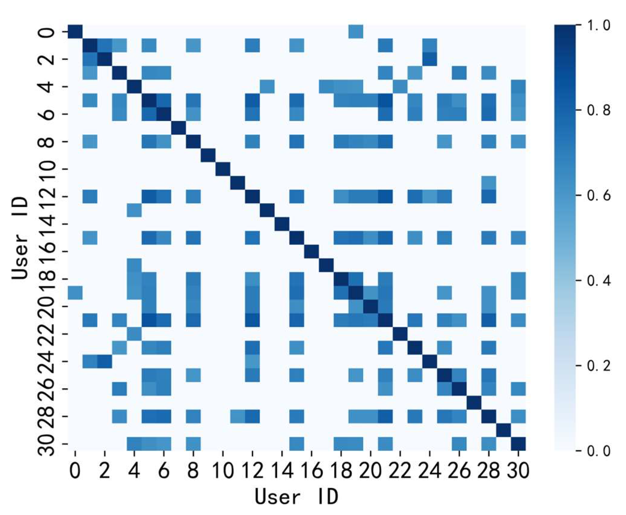
The adjacency matrices for LASTGCN, CASTGCN, and BASTGCN can be found in Appendix A. The autocorrelation analysis results of the data are presented in Appendix B. The results of the autocorrelation analysis of the data are shown in Appendix B, explaining why the input sequence length of 24 was chosen.

The prediction results are shown in

Table 8. Comparison of prediction errors.

Model	MAE/(MW·h)	RMSE/(MW·h)	R2
LASTGCN	0.0316	0.0570	0.9528
CASTGCN	0.0346	0.0613	0.9483
BASTGCN	0.0353	0.0621	0.9477
LSTNet	0.0381	0.0675	0.9370
TCN	0.0427	0.0694	0.9353
LSTM	0.0512	0.0732	0.9318
Informer	0.0520	0.0867	0.9063
Autoformer	0.0502	0.0834	0.9178

, which calculates the average prediction errors for 31 users. Figure 11 displays the daily load prediction results for a randomly selected day on the test set for each model.

From Table 8 and Figure 11, it can be observed that among the prediction models using GCN, the predictive performance follows this order: LASTGCN > CASTGCN > BASTGCN. This indicates that the choice of adjacency matrix can impact the predictive performance of the model. Specifically, LASTGCN shows improvements over CASTGCN in terms of the MAE, RMSE, and R² by 8.67%, 7.01%, and 0.47%, respectively. Compared to BASTGCN, the improvements are 10.48%, 8.21%, and 0.54% for MAE, RMSE, and R², respectively. These enhancements are attributed to the use of a learnable adjacency matrix in the LASTGCN model, which captures the relationships among user sequences more effectively, thereby modeling the complex spatial dependencies between nodes. The CASTGCN model employs a correlation coefficient adjacency matrix that reflects linear correlations among different users. While this matrix aids in capturing node relationships, it falls short when it comes to representing complex nonlinear relationships, resulting in slightly lower predictive performance. The BASTGCN model uses a binary adjacency matrix, which yields lower predictive accuracy compared to CASTGCN. This is because the binary adjacency matrix, containing only 0 s and 1 s, can only roughly indicate whether a relationship exists between nodes without measuring its strength, thus leading to inferior performance compared to the other two models.

Compared with models without GCN, LASTGCN demonstrates even greater improvements. Specifically, LASTGCN improves over LSTNet by 17.06%, 15.56%, and 1.69% in terms of MAE, RMSE, and R², respectively. Compared to TCN, the improvements are 26.00%, 17.87%, and 1.87% for MAE, RMSE, and R², respectively. Compared to LSTM, the improvements are 38.28%, 22.13%, and 2.25% in MAE, RMSE, and R², respectively. These results indicate that although LSTNet employs convolutional structures capable of capturing relationships among users, its ability to do so is inferior to that of models using GCN. This highlights that GCN, by defining relationships among users through adjacency matrices and leveraging graph structures to model these relationships, surpasses traditional convolutional models in spatial modeling capability. The LSTM and TCN models exhibit the lowest prediction accuracy because they primarily focus on temporal correlations while neglecting inter-user relationships. This limitation hinders their ability to achieve higher predictive accuracy, underscoring the importance of spatial relationships among users in prediction outcomes.

Moreover, the superior accuracy of the proposed LASTGCN model over Transformer-based models like Informer and Autoformer can be attributed to its unique ability to dynamically learn and adapt the relationships between sequences, leveraging a learnable adjacency matrix to effectively model local dependencies crucial for short-term load forecasting. This is particularly significant given the strong temporal and spatial correlations inherent in load data, where understanding and predicting short-term trends are essential. In contrast, Transformer-based models, while powerful in capturing long-range dependencies across sequences due to their attention mechanisms, introduce unnecessary complexity and computational overhead in scenarios where local patterns hold more relevance. This often results in suboptimal performance in short-term forecasting scenarios, where the focus should be on accurately modeling and predicting immediate trends rather than distant future events. Consequently, LASTGCN’s focused and efficient approach to modeling short-term dependencies enables it to outperform Transformer-based models, which may struggle with the additional complexity when it is not warranted by the forecasting horizon.

Figure 12 presents the scatter plots designed to evaluate the predictive performance of the LASTGCN model across different users by comparing predicted values with actual load values. These scatter plots provide a visual means to assess the accuracy of the model for each user, as indicated by the R² values. Generally, Figure 12 shows that the LASTGCN model exhibits strong predictive capabilities, with high R² values for the majority of users, indicating a close alignment between predicted and actual values. However, for some users, the model’s predictions are less accurate, as reflected by lower R² values. This discrepancy might be attributed to the lower similarity in load patterns between these specific users and the broader user base. The unique or less common load patterns for these users can pose challenges for the model and affect its ability to generalize and predict accurately, leading to lower predictive performance for those users.

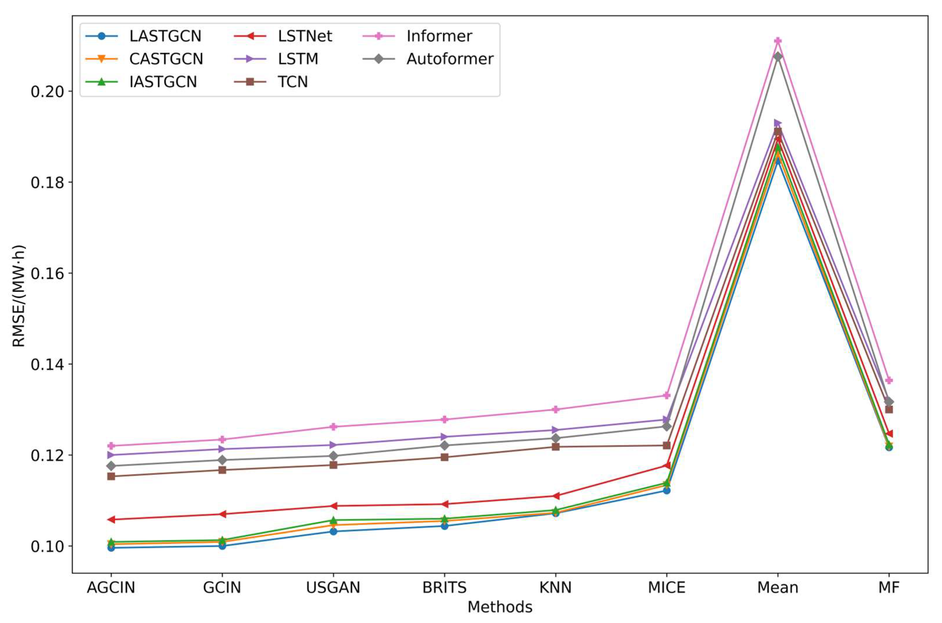
Furthermore, to comprehensively assess the impact of load data imputed by various methods on the accuracy of downstream load forecasting tasks, we selected load data repaired using different imputation techniques at a 40% random missing rate and subjected them to load forecasting models. The resulting RMSE values were carefully evaluated and are presented in Figure 13. As shown in the figure, it is evident that regardless of the specific prediction model employed, the load data imputed by the AGCIN method consistently produced the lowest prediction errors. This consistent performance across different forecasting models underscores the robustness and reliability of AGCIN in effectively repairing load data and, more importantly, highlights its significant positive impact on enhancing the accuracy of downstream load forecasting tasks. The findings further affirm that AGCIN not only excels in the imputation process but also contributes to superior performance in subsequent predictive analyses, making it a crucial tool in managing and forecasting load data with missing values.

3.4.2. Parameter Impact Analysis

In this section, we analyze the impact of L2 regularization and the number of epochs on model performance, as shown in

Table 9. Impact of L2 regularization and epochs.

L2 Regularization	MAE/(MW·h)	RMSE/(MW·h)	R2
0.01	0.0296	0.0531	0.9639
0.001	0.0308	0.0557	0.9591
0.0001	0.0316	0.0570	0.9528
0.00001	0.0302	0.0546	0.9617
Epochs	MAE/(MW·h)	RMSE/(MW·h)	R2
50	0.0342	0.0596	0.8937
100	0.0316	0.0570	0.9528
150	0.0316	0.0568	0.9528
200	0.0314	0.0565	0.9587

.

In analyzing the impact of L2 regularization, we observe a nuanced trend in the model’s performance as the regularization parameter is varied. Initially, increasing the L2 regularization from 0.00001 to 0.0001 resulted in a slight degradation of model performance, as indicated by the increase in RMSE from 0.0546 to 0.0570 and decrease in R² from 0.9617 to 0.9528. This decline suggests that the model may have started to lose some of its capacity to fit the data well as the regularization strength slightly penalized the weight magnitudes, even though the model had not yet begun to overfit significantly.

However, as the L2 regularization parameter is further increased to 0.001 and 0.01, a modest improvement in performance is observed. Specifically, the RMSE decreases to 0.0531, and R² increases to 0.9639 at the highest regularization level of 0.01. This improvement likely reflects the model’s ability to avoid overfitting to the training data while still maintaining sufficient flexibility to capture the underlying patterns in the data.

Overall, the impact of L2 regularization on model performance in this study appears to be relatively minor. This might be due to the model not reaching a point where overfitting was a significant issue, and hence, the regularization did not play as crucial a role in enhancing generalization as it might in more complex models or datasets. This suggests that while L2 regularization is an important parameter to consider, its effects might be subtle unless the model complexity or data characteristics are such that overfitting becomes a pronounced concern.

In analyzing the impact of the number of epochs on model performance, we observe that increasing the epochs from 50 to 100 results in a significant improvement in the model’s accuracy. This is evidenced by the decrease in RMSE from 0.0596 to 0.0570 and the increase in R² from 0.8937 to 0.9528. The marked improvement indicates that the model continues to learn and fit the data better as it is trained for more iterations.

However, as the number of epochs increases to 150 and 200, the performance metrics show minimal changes. The RMSE slightly decreases from 0.0568 to 0.0565, and R² increases marginally from 0.9528 to 0.9587. This trend suggests that the model has likely reached a point of convergence by 100 epochs, where additional training epochs provide diminishing returns in terms of performance enhancement. The model’s learning has stabilized, indicating that it has effectively captured the patterns in the data and further training is not significantly improving the predictive accuracy.

4. Extended Experiments

In this section, we conduct tests using the publicly available UCI-Electricity dataset to verify the generality and robustness of the proposed framework. The dataset can be downloaded from https://github.com/laiguokun/multivariate-time-series-data (accessed on 20 July 2024).

The original dataset contains electricity consumption data for 321 users from 2012 to 2014, with a unit of kWh and a resolution of 1 h. Given the large scale of this dataset and the limitations of our hardware, we chose not to use the entire dataset for our experiments. Instead, we randomly selected 30 users for our analysis and converted the unit from kWh to MWh. The following sections present the imputation and forecasting experiments, with hyperparameters kept consistent with the previous settings.

4.1. Extended Load Imputation Results

In

Table 10. Comparison of imputation errors for extended experiments.

Miss Rate/%	RMSE of Different Imputation Models/(MW·h)
	AGCIN	GCIN	USGAN	BRITS
10	0.0413	0.0422	0.0446	0.0474
30	0.0801	0.0812	0.0840	0.0850
60	0.1348	0.1379	0.1470	0.1500

, we present the imputation results on the extended dataset with random missing rates of 10%, 30%, and 60%. As previously analyzed, deep learning models have demonstrated significant advantages in imputation tasks, so only deep learning models are compared here. AGCIN, the proposed model in this study, continues to show the best performance on the extended dataset. Specifically, as the missing rate increases, AGCIN consistently achieves the lowest RMSE across different missing rates, demonstrating its robustness and effectiveness in handling missing data. This reaffirms the superiority of AGCIN in imputation tasks, even when applied to larger datasets under various missing conditions.

4.2. Extended Load Forecasting Results

Table 11. Comparison of prediction errors for extended experiments.

Model	MAE/(MW·h)	RMSE/(MW·h)	R2
LASTGCN	0.0246	0.0455	0.7991
CASTGCN	0.0257	0.0473	0.7827
BASTGCN	0.0258	0.0477	0.7822
LSTNet	0.0291	0.0457	0.7782
TCN	0.0318	0.0569	0.7599
LSTM	0.0332	0.0587	0.7291
Informer	0.0335	0.0533	0.7248
Autoformer	0.0338	0.0534	0.7253

shows the prediction results on the extended dataset. On this extended dataset, the LASTGCN model continues to demonstrate superior predictive performance. It achieves the lowest MAE (0.0246) and RMSE (0.0455) values among all models tested, with an R² value of 0.7991, which is also higher than that of the other models. This indicates that LASTGCN is more effective when it comes to accurately capturing the characteristics and trends in the load data compared to other models. In contrast, other models such as CASTGCN, BASTGCN, as well as Transformer-based models like Informer and Autoformer, perform less effectively, especially in terms of MAE and RMSE, where none surpass LASTGCN. These results further confirm the leading position of LASTGCN in load forecasting tasks and highlight its advantages in maintaining high predictive accuracy and model robustness.

Overall, these results underscore the robustness and effectiveness of the proposed AGCIN and LASTGCN models, as they consistently deliver superior performance in both imputation and prediction tasks, even when tested on larger datasets.

5. Conclusions

To address the issues of data quality in aggregated load forecasting and the construction of adjacency matrices to capture correlations, this paper presents a graph convolution-based load data restoration and short-term load forecasting approach with a learnable adjacency matrix. The following summary is provided:

To tackle the data quality problem arising from missing load data, this paper introduces the AGCIN model. It represents data as nodes on a graph, employs GCN to capture local correlations between nodes, establishes a local imputation model, and then introduces GAN through adversarial training to create a global imputation model. Experimental verification demonstrates that the combination of local and global imputation enhances imputation accuracy and improves load data quality. The experimental results demonstrate that in random missing scenarios, with a missing rate ranging from 10% to 60%, the RMSE of the AGCIN model ranges from 0.0463 to 0.1465, outperforming other models. In the case of segment missing scenarios, with continuous missing data from 1 day to 9 days, the AGCIN model’s RMSE ranges from 0.0095 to 0.0411, consistently surpassing other models. This proves that combining local and global imputation can enhance imputation accuracy and improve load data quality.

In the context of an aggregated load where specific geographical locations are absent, it becomes challenging to construct an adjacency matrix based on geographical distance for spatio-temporal load forecasting. To address this issue, the paper presents the LASTGCN model. This model considers both temporal and spatial correlations and can adaptively learn interrelationships between different sequences from time series data, obtaining an adjacency matrix. This approach proves effective when predefined graph structures are unattainable. The experimental results show that the prediction errors of LASTGCN in terms of MAE, RMSE, and R² are 0.0316, 0.0570, and 0.9528, respectively, outperforming other prediction models across all three metrics. This indicates that the learnable adjacency matrix provides a flexible and effective method with which to capture the spatial relationships between users. Furthermore, results from various GCN-based prediction models demonstrate that GCN exhibits strong spatial modeling capabilities, and accounting for spatial relationships between users can significantly enhance the accuracy of load forecasting.

Lastly, we must acknowledge some limitations of the current work. Firstly, while data privacy is a significant concern in aggregated load data, particularly as some users may be unwilling to share their data, this manuscript does not address these concerns in depth. The issue of data privacy is crucial because it directly impacts the willingness of users to participate in data collection and sharing, which in turn affects the accuracy and reliability of aggregated load forecasting. In future work, we plan to explore methods such as federated learning and differential privacy to mitigate these concerns. Federated learning, for example, allows for the training of models across decentralized devices or servers holding local data samples without exchanging them, thereby preserving user privacy. Similarly, differential privacy techniques can ensure that the output of the model does not reveal specific information about individual users, even if the data are aggregated.

Secondly, the scale of the data is an issue. For deep learning, larger datasets (both temporally and spatially) are beneficial for model training and validation of generalization. Therefore, in future efforts, we will consider using larger-scale datasets.

Moreover, we are committed to developing a more versatile imputation–prediction framework and extending it to a broader range of potential application scenarios, including the forecasting of other types of loads, such as wind and solar renewable energy. Extending our framework to these domains will allow us to assess its effectiveness in predicting the highly variable and weather-dependent nature of renewable energy sources.

By addressing data privacy concerns through advanced methodologies like federated learning and differential privacy, we believe our future work will make significant strides in both protecting user data and improving the robustness and applicability of our forecasting models. These advancements will be crucial for ensuring that our models can be widely adopted in practical applications, including renewable energy forecasting, while maintaining the trust and participation of users.

References

1. Li, M.; Wang, Y. Power Load Forecasting and Interpretable Models Based on GS XGBoost and SHAP. J. Phys. Conf. Ser. 2022, 2195, 012001. [Google Scholar] [CrossRef]
2. Zhu, J.; Wang, Y.; Li, M.; Chen, Z.; Li, Z.; Xiong, J. Review and Prospect of Data-Driven Techniques for Load Forecasting in Integrated Energy Systems. Appl. Energy 2022, 321, 119269. [Google Scholar] [CrossRef]
3. Chen, Y.; Zhou, J.; Zhang, X.; Tang, J.; Zhang, Y. Day-Ahead Load Forecast Based on Conv2D-GRU_SC Aimed to Adapt to Steep Changes in Load. Energy 2024, 302, 131814. [Google Scholar] [CrossRef]
4. Park, D.C.; El-Sharkawi, M.A.; Marks, R.J.; Atlas, L.E.; Damborg, M.J. Electric Load Forecasting Using an Artificial Neural Network. IEEE Trans. Power Syst. 1991, 6, 442–449. [Google Scholar] [CrossRef]
5. Lee, K.Y.; Cha, Y.T.; Park, J.H. Short-Term Load Forecasting Using an Artificial Neural Network. IEEE Trans. Power Syst. 1992, 7, 124–132. [Google Scholar] [CrossRef]
6. Chen, S.-T.; Yu, D.C.; Moghaddamjo, A.R. Weather Sensitive Short-Term Load Forecasting Using Nonfully Connected Artificial Neural Network. IEEE Trans. Power Syst. 1992, 7, 1098–1105. [Google Scholar] [CrossRef]
7. Aurangzeb, K.; Haider, S.I.; Alhussein, M. Individual Household Load Forecasting Using Bi-Directional LSTM Network with Time-Based Embedding. Energy Rep. 2024, 11, 3963–3975. [Google Scholar] [CrossRef]
8. Lin, J.; Cao, Z.; Li, X.; Fan, M.; Wu, X. Short-Term Load Forecasting Based on LSTM Networks Considering Attention Mechanism. Int. J. Electr. Power Energy Syst. 2022, 137, 107818. [Google Scholar] [CrossRef]
9. Wang, Y.; Yan, G.; Li, K.; Liu, X. Short-Term Load Forecasting for Industrial Customers Based on TCN-LightGBM. IEEE Trans. Power Syst. 2020, 36, 1984–1997. [Google Scholar] [CrossRef]
10. Zhang, T.; Li, Y.; Zhu, W.; Liu, Y.; Zhao, D.; Xu, S. A Hybrid Electric Vehicle Load Classification and Forecasting Approach Based on GBDT Algorithm and Temporal Convolutional Network. Appl. Energy 2023, 351, 121768. [Google Scholar] [CrossRef]
11. Zhang, Z.; Liu, X.; Zhang, C.; Han, J.; Yu, S. General Short-Term Load Forecasting Based on Multi-Task Temporal Convolutional Network in COVID-19. Int. J. Electr. Power Energy Syst. 2023, 147, 108811. [Google Scholar] [CrossRef]
12. Lai, G.; Chang, W.C.; Yang, Y.; Liu, H. Modeling Long-and Short-Term Temporal Patterns with Deep Neural Networks. In Proceedings of the 41st International ACM SIGIR Conference on Research & Development in Information Retrieval, New York, NY, USA, 8–12 July 2018; pp. 95–104. [Google Scholar]
13. Zhang, S.; Chen, R.; Cao, J.; Tan, J. A CNN and LSTM-Based Multi-Task Learning Architecture for Short and Medium-Term Electricity Load Forecasting. Electr. Power Syst. Res. 2023, 222, 109507. [Google Scholar] [CrossRef]
14. Wang, Y.; Rui, L.; Ma, J. A Short-Term Residential Load Forecasting Scheme Based on the Multiple Correlation-Temporal Graph Neural Networks. Appl. Soft Comput. 2023, 146, 110629. [Google Scholar] [CrossRef]
15. Lin, W.; Wu, D.; Boulet, B. Spatial-Temporal Residential Short-Term Load Forecasting via Graph Neural Networks. IEEE Trans. Smart Grid 2021, 12, 5373–5384. [Google Scholar] [CrossRef]
16. Bentsen, L.Ø.; Bakker, S.J.; Sartori, I. Spatio-Temporal Wind Speed Forecasting Using Graph Networks and Novel Transformer Architectures. Appl. Energy 2023, 333, 120565. [Google Scholar] [CrossRef]
17. Zang, H.; Zheng, L.; Liu, J.; Zhang, X.; Xia, Y. Multi-Site Solar Irradiance Forecasting Based on Adaptive Spatiotemporal Graph Convolutional Network. Expert Syst. Appl. 2024, 236, 121313. [Google Scholar] [CrossRef]
18. Zhou, H.; Zhang, S.; Peng, J.; Zhang, S.; Li, J.; Xiong, H.; Zhang, W. Informer: Beyond Efficient Transformer for Long Sequence Time-Series Forecasting. Proc. AAAI Conf. Artif. Intell. 2021, 35, 11106–11115. [Google Scholar] [CrossRef]
19. Wu, H.; Xu, J.; Wang, J.; Long, M.; Jiang, J.; Li, Z. Autoformer: Decomposition Transformers with Auto-Correlation for Long-Term Series Forecasting. Adv. Neural Inf. Process. Syst. 2021, 34, 22419–22430. [Google Scholar]
20. Zeng, A.; Chen, M.; Zhang, L.; Xu, Q. Are Transformers Effective for Time Series Forecasting? Proc. AAAI Conf. Artif. Intell. 2023, 37, 11121–11128. [Google Scholar] [CrossRef]
21. Han, D.; Liu, X.; Zhang, H.; Yu, X.; Liu, J.; Liu, Y. Day-Ahead Aggregated Load Forecasting Based on Household Smart Meter Data. Energy Rep. 2023, 9, 149–158. [Google Scholar] [CrossRef]
22. Li, K.; Wang, Y.; Li, X.; Zhao, Y.; Li, H. Online Transfer Learning-Based Residential Demand Response Potential Forecasting for Load Aggregator. Appl. Energy 2024, 358, 122631. [Google Scholar] [CrossRef]
23. Wang, J.; Liang, X.; Fan, C.; Li, Y.; Zhang, Y.; Liu, X. Aggregated Large-Scale Air-Conditioning Load: Modeling and Response Capability Evaluation of Virtual Generator Units. Energy 2023, 276, 127570. [Google Scholar] [CrossRef]
24. Lindberg, K.B.; Bakker, S.J.; Sartori, I. Modelling Electric and Heat Load Profiles of Non-Residential Buildings for Use in Long-Term Aggregate Load Forecasts. Util. Policy 2019, 58, 63–88. [Google Scholar] [CrossRef]
25. Yu, H.; Zhou, Y.; Zhang, W.; Li, Z.; Tang, Y.; Liu, L.; Wang, J. Privacy-Preserving Demand Response of Aggregated Residential Load. Appl. Energy 2023, 339, 121018. [Google Scholar] [CrossRef]
26. Li, Y.; Yu, R.; Shahabi, C.; Liu, Y. Diffusion Convolutional Recurrent Neural Network: Data-Driven Traffic Forecasting. In Proceedings of the International Conference on Learning Representations, Vancouver, BC, Canada, 30 April–3 May 2018. [Google Scholar]
27. Bertsimas, D.; Pawlowski, C.; Zhuo, Y.D. From Predictive Methods to Missing Data Imputation: An Optimization Approach. J. Mach. Learn. Res. 2018, 18, 1–39. [Google Scholar]
28. Acuna, E.; Rodriguez, C. The Treatment of Missing Values and Its Effect on Classifier Accuracy. In Classification, Clustering, and Data Mining Applications, Proceedings of the Meeting of the International Federation of Classification Societies (IFCS), 15–18 July Chicago, IL, USA, 2004; Illinois Institute of Technology: Chicago, IL, USA, 2004; pp. 639–647. [Google Scholar]
29. Shahid, F.; Wang, S.; Pan, J.; Saleem, F.; Rehmani, M.H. 1D Convolutional LSTM-Based Wind Power Prediction Integrated with PkNN Data Imputation Technique. J. King Saud Univ. Comput. Inf. Sci. 2023, 35, 101816. [Google Scholar] [CrossRef]
30. Sareen, K.; Tiwari, P.K.; Awan, U.K.; Verma, N.K. An Imputation and Decomposition Algorithms Based Integrated Approach with Bidirectional LSTM Neural Network for Wind Speed Prediction. Energy 2023, 278, 127799. [Google Scholar] [CrossRef]
31. Hallam, A.; Mukherjee, D.; Chassagne, R. Multivariate Imputation via Chained Equations for Elastic Well Log Imputation and Prediction. Appl. Comput. Geosci. 2022, 14, 100083. [Google Scholar] [CrossRef]
32. Goodfellow, I.; Pouget-Abadie, J.; Mirza, M.; Xu, B.; Warde-Farley, D.; Ozair, S.; Courville, A.; Bengio, Y. Generative Adversarial Nets. In Proceedings of the Advances in Neural Information Processing Systems, Montreal, QC, Canada, 8–13 December 2014; Volume 27. [Google Scholar]
33. Qu, F.; Wang, S.; Yang, L.; Zhang, W.; Ding, Y. A Novel Wind Turbine Data Imputation Method with Multiple Optimizations Based on GANs. Mech. Syst. Signal Process. 2020, 139, 106610. [Google Scholar] [CrossRef]
34. Kosana, V.; Teeparthi, K.; Madasthu, S. A Novel and Hybrid Framework Based on Generative Adversarial Network and Temporal Convolutional Approach for Wind Speed Prediction. Sustain. Energy Technol. Assess. 2022, 53, 102467. [Google Scholar] [CrossRef]
35. Zhang, W.; Chen, S.; Liu, H.; Li, H.; Cui, B. SolarGAN: Multivariate Solar Data Imputation Using Generative Adversarial Network. IEEE Trans. Sustain. Energy 2020, 12, 743–746. [Google Scholar] [CrossRef]
36. Spinelli, I.; Scardapane, S.; Uncini, A. Missing Data Imputation with Adversarially-Trained Graph Convolutional Networks. Neural Netw. 2020, 129, 249–260. [Google Scholar] [CrossRef] [PubMed]
37. Kipf, T.N.; Welling, M. Semi-Supervised Classification with Graph Convolutional Networks. arXiv 2016, arXiv:1609.02907. [Google Scholar]
38. Eirola, E.; Hinkkanen, M.; Kärkkäinen, T.; Seppänen, T. Distance Estimation in Numerical Data Sets with Missing Values. Inf. Sci. 2013, 240, 115–128. [Google Scholar] [CrossRef]
39. Talwalkar, A.; Kumar, S.; Mohri, M. Large-Scale SVD and Manifold Learning. J. Mach. Learn. Res. 2013, 14, 3129–3152. [Google Scholar]
40. Battaglia, P.W.; Hamrick, J.B.; Bapst, V.; Sanchez-Gonzalez, A.; Zambaldi, V.; Malinowski, M.; Tacchetti, A.; Raposo, D.; Santoro, A.; Faulkner, R.; et al. Relational Inductive Biases, Deep Learning, and Graph Networks. arXiv 2018, arXiv:1806.01261. [Google Scholar]
41. Gondara, L.; Wang, K. Multiple Imputation Using Deep Denoising Autoencoders. arXiv 2017, arXiv:1705.02737. [Google Scholar]
42. Gulrajani, I.; Ahmed, F.; Arjovsky, M.; Dumoulin, V.; Courville, A. Improved Training of Wasserstein GANs. In Proceedings of the Advances in Neural Information Processing Systems, Long Beach, CA, USA, 4–9 December 2017; Volume 30. [Google Scholar]
43. Wu, Z.; Pan, S.; Long, G.; Jiang, J.; Chang, X.; Zhang, C. Connecting the Dots: Multivariate Time Series Forecasting with Graph Neural Networks. In Proceedings of the 26th ACM SIGKDD International Conference on Knowledge Discovery & Data Mining, Virtual Event, 6–10 July 2020. [Google Scholar]
44. Gasteiger, J.; Bojchevski, A.; Günnemann, S. Predict Then Propagate: Graph Neural Networks Meet Personalized PageRank. arXiv 2018, arXiv:1810.05997. [Google Scholar]
45. Abu-El-Haija, S.; Perozzi, B.; Kapoor, A.; Lee, J. MixHop: Higher-Order Graph Convolutional Architectures via Sparsified Neighborhood Mixing. In Proceedings of the International Conference on Machine Learning, Long Beach, CA, USA, 9–15 June 2019; pp. 21–29. [Google Scholar]
46. Oord, A.v.d.; Dieleman, S.; Zen, H.; Simonyan, K.; Vinyals, O.; Graves, A.; Kalchbrenner, N.; Senior, A.; Kavukcuoglu, K. WaveNet: A Generative Model for Raw Audio. arXiv 2016, arXiv:1609.03499. [Google Scholar]
47. Miao, X.; Wu, Y.; Wang, J.; Gao, Y.; Mao, X.; Yin, J. Generative Semi-Supervised Learning for Multivariate Time Series Imputation. Proc. AAAI Conf. Artif. Intell. 2021, 35, 8983–8991. [Google Scholar] [CrossRef]
48. Cao, W.; Wang, D.; Li, J.; Zhou, H.; Li, L.; Li, Y. BRITS: Bidirectional Recurrent Imputation for Time Series. Adv. Neural Inf. Process. Syst. 2018, 31, 6775–6785. [Google Scholar]
49. Ranjbar, M.; Moradi, P.; Azami, M.; Jalili, M. An Imputation-Based Matrix Factorization Method for Improving Accuracy of Collaborative Filtering Systems. Eng. Appl. Artif. Intell. 2015, 46, 58–66. [Google Scholar] [CrossRef]
50. Hochreiter, S. Long Short-Term Memory. Neural Comput. 1997, 9, 1735–1780. [Google Scholar] [CrossRef]
51. Bai, S.; Kolter, J.Z.; Koltun, V. An Empirical Evaluation of Generic Convolutional and Recurrent Networks for Sequence Modeling. arXiv 2018, arXiv:1803.01271. [Google Scholar]
Figure 1. Relationship between local and global imputation.
Energies 17 04583 g001
Figure 2. Local imputation model based on GCN.
Energies 17 04583 g002
Figure 3. Global imputation model based on GAN.
Energies 17 04583 g003
Figure 4. Structure diagram of LASTGCN model.
Energies 17 04583 g004
Figure 5. Structure diagram of mix-hop propagation layer.
Energies 17 04583 g005
Figure 6. Structure diagram of mix-hop convolutional layer.
Energies 17 04583 g006
Figure 7. Imputation error results for random missing data.
Energies 17 04583 g007
Figure 8. Imputation error results for missing data fragments.
Energies 17 04583 g008
Figure 9. Imputation results over a specific time period.
Energies 17 04583 g009
Figure 10. Data distribution before and after imputation.
Energies 17 04583 g010
Figure 11. Comparison of prediction results on a day.
Energies 17 04583 g011
Figure 12. Scatter plots of LASTGCN prediction results.
Energies 17 04583 g012
Figure 13. Influence of different imputation methods on prediction errors.
Energies 17 04583 g013