Abstract
This paper presents a novel approach to determining the ampacity of DC and AC railway overhead contact lines, considering both operational and design factors. The ampacity of contact lines is influenced by several design parameters, including materials, cross section and the number of catenary and contact wires, etc. Additionally, the permissible long-term and short-term current values, which correspond to the permissible temperatures defined by EN 50119:2020, are affected by operational factors such as ambient temperature, solar radiation, heat exchange conditions, wind speed, wear of contact wires. Existing methods for determining the ampacity of overhead contact lines often fail to account adequately for these critical factors and lack the necessary procedures to calculate the 30 min ampacity required by EN 50119:2020. In response, the method proposed in this study adapts the procedures of IEEE 738-2012 to the specific needs of railway contact lines, taking into account the effect of contact wire wear on current distribution and overall ampacity. The proposed method offers a more realistic and practical approach to determining the ampacity of contact lines, thereby enhancing the reliability and efficiency of the traction power supply infrastructure. This method could be useful for railway infrastructure managers to ensure the safe and efficient operation under varying environmental and operational conditions.
1. Introduction
The railway overhead contact line is one of the factors that limit the possibility of increasing the speed and length of trains on electrified railway lines. The current consumed by the rolling stock is the main factor determining the temperature mode of the contact lines. At the design stage, an important issue is to calculate the ampacity of the contact lines. During operation, it is crucial to ensure that the temperature of the contact lines does not exceed the permissible level. The overhead contact line is a component of the electric traction power supply system, designed to supply the vehicle with electricity of the required parameters, including current of a specified value. According to the Technical Specification of Interoperability TSI Energy [,] and standards [], trains can consume from a power supply system 3 kV DC current up to 4 kA, for AC traction power supply system up to 1.5 kA. Current of these values should be transmitted through the overhead contact line without adverse effects on its technical condition, which is related to ampacity of the overhead contact line [].
Choosing excessively large cross sections for contact lines leads to oversized dimensions and unnecessary capital expenses. The choice of insufficient cross sections of wires can lead to a decrease in the reliability of the contact lines. The currents flowing through the wires generate heat, leading to energy loss and causing their temperature to rise above the ambient level []. This has two consequences:
- -
- The tension and ordinates of the sag curves of freely suspended overhead contact wires and uncompensated chain suspension wires change. In addition, the droppers, clamps and brackets become misaligned in the latter;
- -
- Accelerated ageing of wires, which is expressed in a decrease in the elastic limit and breaking tension and, consequently, in a decrease in the safety margin of the structure.
If we compare the nature of the current load of railway contact lines with the nature of the load of power system lines, we can conclude that the load of contact lines differs cardinally, it has a dynamic character. The current load of the contact line depends on the position of the train on the inter-substation section, the horizontal and vertical profile of the railway line, the speed of the train, train working mode (traction, coasting, regenerative braking, etc.), the wind speed, and the power supply circuit of the given section. The use of conductor ampacity for conductor size selection can lead to wrong conductor choices when the current is fluctuating, as always occurs in railway lines. Current profile of contact lines usually contains high and long-lasting peaks resulting in high temperatures [].
The ampacity of a current path depends on a number of factors, which include []:
- -
- the material from which the current path is made;
- -
- maximum allowable temperature increments;
- -
- shape and dimensions;
- -
- surface condition;
- -
- current path operating environment (air, gas, oil, solid insulation);
- -
- heat sources in the neighborhood;
- -
- flow of cooling medium.
In the scientific literature, there are many publications which are devoted to different methods of determining the ampacity of power system lines. For example, in [] was presented a method that uses Extreme Learning Machine (ELM) to predict the capacity of overhead power lines. By using historical weather data, this method provides quick and accurate forecasts, which help in optimizing the operation of power systems. The study also pointed out the limitations of traditional Static Thermal Rating (STR), which often underestimates the actual capacity of transmission lines due to conservative weather assumptions. In [], the authors introduced a Quantile Regression Neural Network (QRNN) model to predict the ampacity of overhead power lines. Unlike traditional methods, the QRNN model provides a range of possible outcomes, helping operators make more informed decisions. By incorporating real-time weather data, this method gives a more accurate and usually higher estimate of transmission capacity, which is crucial for managing the growing demand for renewable energy. The work [] is devoted to improving the safety and efficiency of power lines by predicting their ampacity more accurately by dynamic line rating (DLR) methods. DLR methods adjust line ampacity based on real-time weather data. The study emphasizes the importance of using reliable probabilistic forecasts to prevent overheating and other risks, especially in challenging environments where weather can change quickly. The work [] is also devoted to the use of Dynamic Line Ratings (DLRs) to optimize the current capacity of overhead transmission lines based on actual weather conditions. The authors analyze the benefits and drawbacks of Artificial Intelligence-based models to calculate the ampacity. All of the aforementioned methods focus on assessing the ampacity of energy system lines. However, these methods are not suitable for determining the ampacity of railway contact lines due to the specific design and operational characteristics of these lines.
Some authors have focused on the development of thermal models of line heating. The work [] explores how natural convection cools power lines when the wind is not blowing, which is crucial for maintaining safety. The results are also compared with CIGRE, IEEE, and IEC guidelines. In the field of railways contact line, it is necessary to mention the following scientific works. The work [] proposed a methodology for calculating the thermal heating of DC contact lines. It introduces a comprehensive mathematical model that accounts for various elements such as wires, current-carrying clamps, etc. This model considers the nonlinear material properties dependent on temperature, uneven wear along the contact wire, and external factors like solar radiation and convective and radiative heat exchange. It enables the analysis of both steady-state and transient electrical currents, covering scenarios like transit, current collection, stationary power consumption, overloads, and short circuits. Work [] is also devoted to the development of a thermal model for the heating of railway contact lines. This research utilizes a combination of statistical and physical modeling to predict the temperature under different operational conditions. This hybrid approach aims to improve the accuracy of predictions, which are essential for preventing overheating and potential failures in the contact line system. The listed works also do not provide computational procedures to determine the ampacity of contact lines considering design and operational parameters. Let us examine the design and operational characteristics of railway contact lines.
A catenary is a current circuit in which electrically interconnected contact wires and catenary wire(s) are the main carriers of electricity. Contact wires and catenary wire(s) work in parallel and are connected laterally through droppers, distance brackets, suspension elements, and other electrical and mechanical connections made of conductive materials. The catenary is a current track operating in atmospheric air, and its conducting elements are made of copper or its alloys and are approximately circular in shape.
Depending on the temperature and the contact wire material, operation of contact wires at elevated temperatures can reduce their strength. Prolonged heating of cold-drawn copper wire causes the crystalline microstructure to regain its pre-cold-drawn state. This transition to a stable crystalline microstructure is called recrystallization and is accompanied by the restoration of the physical properties typical of cold-drawn contact wire to those of annealed copper. When the recrystallization temperature is exceeded, the microstructure changes and is accompanied by a loss of tensile strength. In this process, the crystalline grains again assume a stable circular shape, and the microstructure formed by cold drawing is almost completely transformed []. The reduction in tensile strength can be assessed by the annealing point. This is the temperature at which the material can be held for an hour, when its tensile strength drops by half the difference between the original high tensile strength and the final low tensile strength of the material, resulting from exposure to high temperatures for a long time. This process is a function of both the temperature and the period of time the material is held at that temperature. The loss of tensile strength of copper wires due to heating increases with the length of time the material is operated at high temperatures, the conversion factor, and the purity of the copper. Using copper with silver or magnesium significantly delays the loss of tensile strength, allowing doped contact wires to operate at higher temperatures and tensile loads than those made from Cu-ETP (pure copper).
During the operation of the overhead contact lines, the contact wires wear out (on Polish railways, the permissible average wear of the contact wires is 30%), which affects the redistribution of currents in the wires of the overhead contact lines. The ampacity of the contact line will be determined by the element in which the current reaches the maximum permissible value faster during the increasing of the load.
Below is a brief review of existing models of current distribution in elements of the contact line, developed at different periods of time and applied at the stage of design of contact lines.
- Natural Current Distribution Model. In this model, the current is distributed among the contact wire, catenary wire, and reinforcing wires in inverse proportion to their resistance. Transverse electrical connectors and other elements are not considered, which limits the accuracy of the model [].
- Linear Analytical Model. This model uses simplified assumptions, such as zero resistance of electrical connectors and representation of the contact line by two wires. It is suitable for choosing the location of transverse electrical connectors but requires improvements for analyzing other wires [].
- A model proposed by K.L. Kostyuchenko. In this model, the current distribution in the reinforcing wire is calculated more accurately, but results may vary due to unaccounted droppers and other elements [].
- A model with an Infinite Number of Droppers. All connections between contact wires and catenary wires are expressed through the equivalent transverse resistance, which allows for considering local resistance differences. This model is not suitable for catenaries with RW and analyzing local connections [,].
- Model KONT-3. This software considers the topology of the contact suspension. This model cannot calculate the elements heating during passage of the train [].
- UKS-Current Program complex. In this program complex, the contact line is represented as a spatial graph, allowing flexible geometry setting and result output [,].
- Finite Element Model (FEM). This model uses Comsol Multiphysics to import geometry and solve differential equations. The model considers the movement of electric rolling stock (ERS), wire heating, and resistance changes with temperature, making it the most accurate but resource-intensive [,].
- Model of current distribution in the contact line based on EasyEDA ver. 2.2.26.6 software package [].
The calculation of current distribution in AC overhead contact lines is a more complex task due to the need to take into account magnetic couplings between overhead contact line elements, nonlinearity of rail resistance under AC current, uneven current distribution in the rails, and overhead contact line in the sections between substations. In the case of AC electrification, due to the magnetic couplings between the various elements of the overhead contact line, the following methodology was used to estimate the current distribution to replace the conductors and rails with surrogate conductors [,,]. The inclusion of droppers in models describing the current distribution in contact lines in AC traction power systems leads to a significant complication of the models. On the other hand, as in the case of DC electrification, droppers have a negligible effect on the current distribution in the components of the contact line.
The impedance of an AC overhead power supply system consists of the intrinsic impedance of the overhead line and traction power feeder line (in the case of a 2 × 25 kV power system) and the mutual impedance of the ground-rails, ground-traction power feeder line and traction power feeder line-rails. Accidental couplings of ground-rails and ground-overhead line induce eddy currents in the ground. The earth-overhead line coupling plays the dominant role in generating eddy currents [].
The analyzed methods of calculating the ampacity of energy system lines cannot be used directly for contact lines due to the design and operational features of the latter. For the needs of railway infrastructure managers, a more simplified methodology is needed to determine the ampacity of contact lines, taking into account design and operational factors that meet the requirement of EN 50119:2020. This is especially significant in relation to major railway projects in Europe, such as the Central Communication Port (CPK) and Rail Baltica. As modern railway networks evolve, there is an increasing demand for higher train speeds, longer train sets, and enhanced operational reliability. These demands place significant stress on the existing traction power infrastructure, particularly on the overhead contact lines. Consequently, accurately determining the ampacity of these lines is essential both during the design phase and throughout their operational life to prevent overheating and ensure the system’s safety and durability.
Based on the presented methods analysis, it was identified that the most appropriate method that allows to determine the ampacity of wires with engineering accuracy (sufficient for the needs of railway infrastructure managers) is the method based on the IEEE 738-2012 standard. To determine the ampacity of catenary lines, the authors of this paper use the approach of standard IEEE 738-2012 [], extending this method to multiconductor lines. In this article, the methodology given in the standard is adapted to the determination of ampacity of contact lines taking into account the requirements of standard PN-EN 50119:2020 [] (this standard requires calculation not only long-time and 1 s ampacities but also 30 min ampacity of the catenary lines).
The objective of this article is to develop an adapted method based on the IEEE 738-2012 standard for calculating the ampacity of contact lines, taking into account operational and design factors. To achieve this objective, the authors of the article proposed:
- scientific approaches to determining the distribution of currents in the elements of contact lines on direct and alternating current;
- an adapted method for determining the ampacity of contact lines taking into account the requirements of PN-EN 50119:2020 [].
This paper presents the results of calculation of the ampacity of contact lines operated on Polish railways and planned for future operation with AC electrification.
2. Materials and Methods
2.1. Matrix of Variables Defining Conditions Affecting Catenaries Ampacity
This section presents the main design features of the contact lines of Polish railways, as well as operational parameters.
In Table 1 of EN 50119:2020 [] are included the permissible temperatures for different materials of contact line conductors:
- -
- maximum long-term temperature;
- -
- short-term maximum temperature (duration up to 30 min);
- -
- short-term maximum temperature (duration up to 1 s).
The permissible long-term and short-term current values, which correspond to the permissible temperatures according to EN 50119:2020, are determined by the ambient temperature, solar power, heat exchange conditions, and the time of current consumption (travel speed). The mechanical parameters of the current-consuming system, including the contact wire, limit the value of the current drawn. The specified current ampacity (in effect, thermal capacity) applies to a given contact wire design. Among the main variables affecting power losses are current, time, heat capacity, thermal conductivity, convection and radiation []. Usually, unfavorable conditions (wind speed, ambient temperature, and solar radiated power) are assumed.
The following are the values of the grouped variables considered in this paper to determine the ampacity of the catenaries:
- Design parameters
- 1.1.
- 3 kV traction power supply system
- -
- Cross section of catenary wires—95 mm2, 120 mm2, 150 mm2;
- -
- Cross section of contact wires—100 mm2, 150 mm2;
- -
- Material of catenary wire—Cu;
- -
- Material of contact wires—CuETP, CuAg0.10 (alloy of copper and 0.10% silver), CuMg0.02 (alloy of copper and 0.02% magnesium);
- -
- Numbers of catenary and contact wires
- The number of catenary wires—1 and 2;
- The number of contact wires—1 and 2.
- 1.2.
- 1 × 25 kV and 2 × 25 kV traction power supply systems
- -
- Cross section of catenary wires—70 mm2, 95 mm2, 120 mm2;
- -
- Cross section of contact wires—100 mm2, 120 mm2, 150 mm2;
- -
- Cross section of traction power feeder line (for 2 × 25 kV), mm2—120, 150, 185, 240, 300;
- -
- Material of catenary wires—CuSn (Bz);
- -
- Material of contact wires—CuETP, CuAg0.10, CuMg0.2 (alloy of copper and 0.2% magnesium), CuMg0.5 (alloy of copper and 0.5% magnesium), CuSn0.2 (alloy of copper and 0.2% selenium);
- -
- Traction power feeder line material (for 2 × 25 kV)—Al;
- -
- Numbers of catenary wires and contact wires
- The number of catenary wires—1;
- number of contact wires—1.
- Operating parameters
- -
- Average annual wind speed in the direction perpendicular to the axis of the wires Vw, m/s—0.6, 2,
- -
- Average wear of contact wires, %—5, 10, 15, 20, 30;
- -
- Ambient temperature: +40 °C.
2.2. Adopted Methodology for Calculation of Current Ampacity of Wires
This section provides theoretical approaches for determining the long-term, 30 min, and 1 s ampacity of wires. As noted, the IEEE 738-2012 standard does not contain information on how to determine the 30 min ampacity of wires. Whereas according to EN 50119:2020, there is a need to determine the 30 min ampacity. In the operation of contact lines, the 30 min ampacity is used for verifying the energy subsystem for compliance with TSI ENE requirements. Therefore, based on the heat balance equation, a formula is proposed to determine the 30 min ampacity.
The ampacity of catenary lines can be obtained from the ampacity of individual conductors. In this study, the ampacity of contact lines is calculated according to IEEE 738-2012 []. The evaluation of the conductor’s temperature and current ampacity is based on the conductor’s heat balance, which is affected by the following factors:
- -
- energy introduced by the Joule heat NJ due to the resistance of the conductor;
- -
- energy provided by solar radiation NS;
- -
- energy consumed by magnetic losses NM;
- -
- energy loss by radiation NR;
- -
- energy loss by convection NC.
For reinforced cables and steel-core conductors used in overhead power lines, magnetic losses contribute to the conductor’s temperature rise. In the case of catenary components, they can be neglected. Therefore, the heat balance associated with a unit length of a single cable can be determined using the formula
where mc—the unit weight of the cable,
- C—specific heat (can be selected according to tab.11.5 []),
- T—temperature of the wire,
- dt—derivative with respect to time.
Table 1 shows the allowable temperatures of wires or cables for long-term, short-term, and 1 s operation modes.

Table 1.
Permissible line or conductor temperature according to Table 1 of EN 50119:2020 [].
Energy introduced by Joule heat NJ due to resistance of conductor
where I—rms value of current, A,
—resistance calculated at temperature T, Ω/m.
where —temperature coefficient of resistivity,
—DC resistance at 20 °C, Ω/m.
The energy provided by solar radiation NS is calculated according to IEC 61597 [].
where —standard solar radiation, ,
D—diameter of the cable, m,
—absorption coefficient. For conductors used in contact lines, it can be adopted according to Table 7.1 [].
Energy losses by radiation NR are calculated according to IEC 61597 []:
where —absolute temperature of the conductor, K
T—conductor temperature, °C.
In the calculation of the long-term current ampacity of cables, we take the maximum temperature values of cables according to Table 1 of standard PN-EN 50119:2020 [].
—absolute ambient temperature, K,
—blackbody radiation constant, Stefan–Boltzmann constant,
—emission factor adopted in accordance with Table 7.1 [].
Energy loss by convection NC can be calculated from the formula
—ambient temperature, °C
—Thermal conductivity of air, ) (Table 7.2 [])
—Nusselt number, which in the case of forced convection depends on the Reynolds number according to IEC 61597 [].
The Reynolds number Re is given by the formula
where —wind speed, m/s,
—specific mass of air, kg/m3,
η—dynamic viscosity in N s/m2.
, , η can be obtained from Table 7.2 [] or from Appendix H of IEEE Standard 738-2012 [].
The long-term current ampacity of cables is determined by the equation (simplified as described in [])
As already mentioned, IEEE Standard 738-2012 [] does not contain information on how to determine the 30 min short-term ampacity of catenary wires. This value can be determined using the heat balance Equation (1) as follows.
where —permissible 30 min conductor temperature according to tab.1 of the PN-EN 50119:2020 standard [],
= 30 min =1800 s.
The current ampacity of 1 s short-circuit conductors can be calculated as follows. First, the effective value of the 1 s allowable current is calculated according to the formula
where —effective value of 1 s allowable current, A,
= 1 s—warm-up time,
—specific mass of the cable, ,
—specific resistance at 20 °C, ,
—permissible 1 s cable temperature according to EN 50119:2020 [],
A—cable cross section, .
The value of the initial symmetrical short-circuit current is then calculated . This value reflects the 1 s load capacity of the conductors. For DC conductors and for AC contact line conductors with two-way power supply can be adopted . The 1 s current ampacity of AC contact line conductors with single-sided power supply can be calculated according to EN 60865-1 [] taking into account the recommendations on p. 438 in the work [] according to the formula
In this study, AC electrified rail sections are assumed to be supplied in a one-way arrangement.
2.3. Adapted Methodology for Calculation of Ampacity of Contact Lines
This section presents an adapted methodology for determining the ampacity of contact lines based on IEEE 738-2012. The IEEE methodology is extended to multiconductor lines. It presents approaches to the determination of current distribution in elements of DC and AC contact lines and formulates the principles of determining the ampacity of contact lines in general.
2.3.1. Calculation of Current Distribution in DC Contact Lines
The analysis of current flows in DC contact lines was based on a catenary model. In the proposed model, the components of the catenary are electrically connected to each other, forming a system in which contact wires and supporting rope(s) are the main carriers of electricity. Contact wires and catenary wire(s) operate in parallel and are connected laterally through droppers, distance lugs, suspension elements (slash, overhang and lashing arms), and other electrical and mechanical connections made of conductive materials. The input data for the construction of the contact line models were catalog data [,]. The nodes of the network are all points where at least two elements that make up the model are connected. Since an overhead contact line system operating in a DC system is being considered, only resistive elements are present in the model.
The resistances of the model elements were calculated as follows: the resistances of the suspension elements (Rs) and distance holders (Rr) were determined from the measurements. All measurements were performed on three samples for four values of current, and the average value of all measurements was taken as the final result of the measurements [,]. The resistances of the sections of the suspension cable (RL), the stitch wire “Y” (RLy), and the contact wires (Rpj) were calculated as the product of the resistance of 1 m of wire or cable and the length of the wire or cable between the nodes. To simplify the calculations in the model, the average values of the droppers’ lengths were used to calculate their resistance Rw. The resistance of electrical connections (Re) was determined in a similar manner. All calculations were performed assuming unit values of resistance of wires as in Table 2.
Table 2.
Unit values of wire resistance [,,,].
All calculations were carried out in EasyEDA simulation software based on the through-span model. The span model (screenshot of the window of the simulation software “EasyEDA” [,]) is shown in Figure 1.
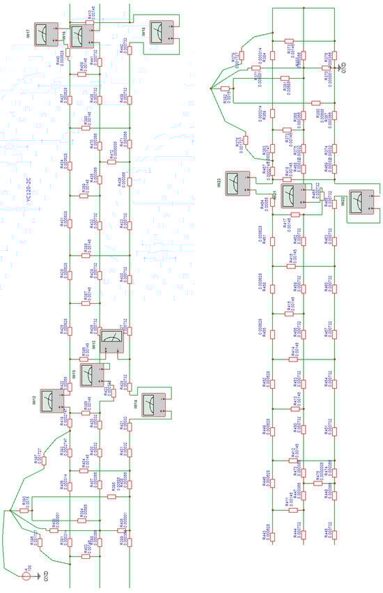
Figure 1.
Model of DC catenary in EasyEDA software.
Conductive and non-conductive droppers are used in catenary systems (only conductive droppers are used in new catenaries).
All droppers have two main functions []:
- -
- maintaining the contact wire at the proper height relative to the track plane;
- -
- withstand the load cycle caused by the passage of trains.
Traditionally, droppers do not perform electrical functions, but conductive droppers are increasingly being used to reduce the potential difference between suspension cables and contact wires.
Calculations of current flow in contact lines with conductive droppers on models have shown that the presence of conductive droppers has a negligible effect on the nature of current flow in contact wires and suspension cables. The model of the contact line with non-conductive droppers is analogous. There is no need to separately analyze their influence on the nature of current distribution in contact wires. Therefore, the influence of droppers can be ignored.
2.3.2. Calculation of Current Distribution in AC Contact Lines
The full unit impedance of a circuit can be represented as the sum of three components—the active electrical resistance of the circuit, the reactance due to an external magnetic field, and the reactance of the circuit due to an internal magnetic field. Given that the catenary consists of multiple conductors and rails, it is necessary to take into account the mutual impedance between all conductor-to-ground and rail-to-ground circuits. The inductances of any circuit due to an external magnetic field L, as well as the coefficients of mutual inductance M between two circuits, including conductor and ground, at the applied current frequencies and suspension heights of the overhead contact line conductors, are determined using the Carson–Pollack formula.
The current in the rails and their impedance are interdependent and variable. It is not possible to take this into account in practical calculations. Therefore, we use an approximate solution, assuming that they are constant along the entire length of the track and equal to their average value. In order to simplify analytical calculations, this study assumes that the track system (consisting of two rails) is replaced by one substitute rail and the contact line conductors by one substitute wire. The assumption that the current in the rails is invariant allows us to practically determine the impedance of the contact line only for two limiting cases, when the transition impedance between the rails and the ground is equal to infinity and when it is equal to zero. To determine the current ampacity of contact lines, we assume that the transition impedance between rail and ground is zero. Below are the formulas used to calculate the current flow in the conductors of the AC contact line.
Full impedance of 1 km of contact line,
where —soil conductance, (in this study assumed for 50 Hz),
—cable resistance, ,
—design radius of the cable, m.
Value of equivalent impedance of 1 km of rails for a single-track section
where —The resistance of 1 km of rail, (in this paper we assume for S60 bus at 50 Hz),
—design radius of the rail, m,
—distance between rails, m.
The value of the equivalent impedance of 1 km of rails for a double-track section
—distance between axes of the I and II tracks, m.
The value of the mutual impedance between conductors n1 and n2,
where —distance between two wires, m.
After eliminating the coupling between the various components of the 1 × 25 kV power system, given the assumption of zero transition impedance between rails and ground [,,] we obtain formulas for calculating the current distribution in the contact wires of the 1 × 25 kV AC contact line.
Part of the current in the contact wire KDjp
Part of the current in the catenary wire KLN
A typical cross section along with geometric parameters of railway lines supplied by the 2 × 25 kV and 1 × 25 kV power systems is shown in Figure 2.
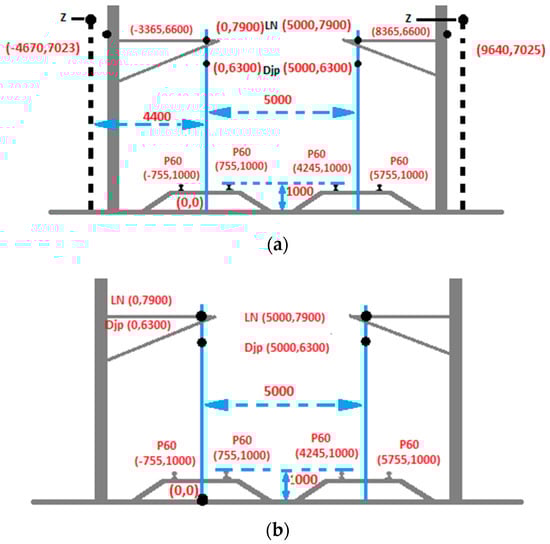
Figure 2.
Typical cross section of a railroad line supplied with alternating current (a) 2 × 25 kV, (b) 1 × 25 kV.
For a 2 × 25 kV traction power supply system, calculations become more complicated due to the presence of a traction power feeder line wire. To simplify the calculations, the contact line is replaced by an equivalent impedance conductor , and the rails are replaced by an equivalent rail. The value of the equivalent impedance of the contact line can be calculated according to the formula []
where —Djp and LN impedances,
—the mutual impedance between Djp and LN.
Part of the current in the traction power feeder line of the 2 × 25 kV power system
where —impedance of the longitudinal power supply.
Part of the current in the contact line
Part of the current in the contact wire of 2 × 25 kV traction power supply system
The part of the current in the catenary wire of the 2 × 25 kV traction power supply system can be calculated according to Equation (18) by substituting the corresponding value of the part of the current in the contact line from Equation (22).
The above calculation methodology allows us to determine the current distribution in the contact line conductors of the 2 × 25 kV power system along the section between the traction substation and the nearest autotransformer in the case of remote location of the train. A typical current distribution in the contact line wires of the 2 × 25 kV power system is shown in Figure 3.
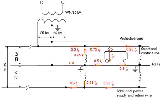
Figure 3.
Typical current distribution in overhead conductors of a 2 × 25 kV power system [].
2.3.3. Principles of Calculating the Ampacity of Contact Line
The ampacity of the AC contact line is determined by calculating the value of the currents flowing through the contact wire Djp, the catenary wire LN, the traction power feeder line Z, and the traction power feeder line under limiting conditions (for the DC contact line, we should take into account Djp, LN, and Y wire). The ampacity is determined by the element that first reaches the limit value. To calculate the current ampacity of the contact line, the following equations are used:
Table 3, Table 4 and Table 5 show the calculated values of the current ampacity of the overhead contact lines according to the above methodology. For the 2 × 25 kV power system, the values of allowable currents for the 30 min short-term mode are not given due to the fact that the normative documents do not specify the temperature limits for the 30 min short-term load mode for aluminum wires (the traction power feeder line is made of AFL-6 material).
Table 3.
Ampacity of DC contact lines.
Table 4.
Current ampacity of AC contact lines of the 1 × 25 kV traction power supply system.
Table 5.
Current ampacity of AC running networks of the 2 × 25 kV power system with AFL-6 120 mm2 traction power feeder line.
3. Results
Table 3 and Figure 4, Figure 5 and Figure 6 present the results of calculations of ampacity for the contact lines used on Polish railroads obtained by Formulas (23)–(25) for wind speeds of 0.6 m/s and 2 m/s, which are relevant for Polish railroads. The right column of Table 3 shows the weak element of the contact line for wind speeds of 0.6 m/s as the most complex in terms of the ampacity of the contact line.
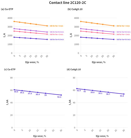
Figure 4.
Ampacity of the contact line 2C120-2C (a,b) long-term and short-term ampacity of contact line with contact wire made from Cu-ETP and CuAg0.10 accordingly; (c,d) 1 s ampacity for contact line with contact wire made from Cu-ETP and CuAg0.10 accordingly.
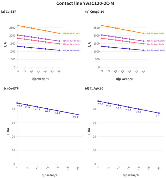
Figure 5.
Ampacity of the contact line YwsC120-2C-M (a,b) long-term and short-term ampacity for contact line with contact wire made from Cu-ETP and CuAg0.10 accordingly; (c,d) 1 s ampacity for contact line with contact wire made from Cu-ETP and CuAg0.10 accordingly.
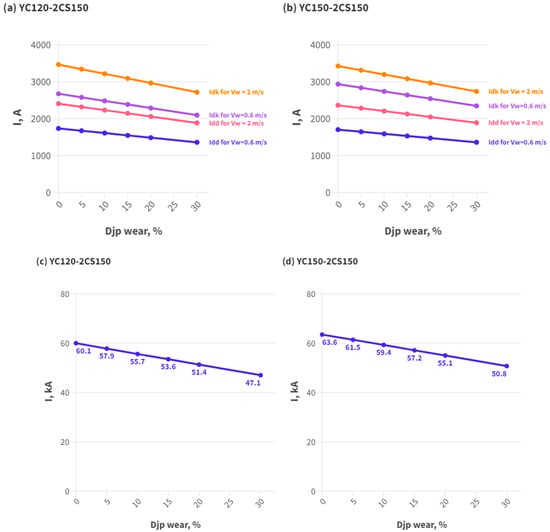
Figure 6.
Long-term, short-term, and 1 s ampacity of the contact lines (a,c) YC120-2CS150 (material of the contact wire is CuAg0.10); (b,d) YC150-2CS150 (material of the contact wire is CuAg0.10).
The results presented in Table 4 and Table 5 provide a comprehensive analysis of the current ampacity for AC contact lines in both the 1 × 25 kV and 2 × 25 kV traction power supply systems. These results highlight several key findings related to the distribution of currents, the influence of various materials, and the impact of operational conditions such as wind speed and contact wire wear.
Table 4 details the ampacity of AC contact lines for the 1 × 25 kV traction power system. The data illustrate that the distribution of currents is significantly influenced by the material of the contact wires. Contact wires made from CuAg0.10, CuSn0.2, CuMg0.2, and CuMg0.5 demonstrate varying ampacities. For instance, the use of CuAg0.10 material consistently results in higher ampacity values compared to other materials, owing to its superior thermal properties and lower electrical resistivity. The ampacity values decrease progressively with the increase in contact wire wear, which indicates that wire wear is a critical factor in determining the operational efficiency of the contact lines.
For the 2 × 25 kV traction power supply system (Table 5), similar trends are observed. The data underscore the importance of the traction power feeder line, particularly those made of AFL-6 120 mm2, which serves as a limiting factor for the overall ampacity of the system.
The proposed method for calculating the ampacity of DC and AC contact lines offers a significant improvement by taking into account the wear of contact wires, which the IEEE 738-2012 standard does not consider.
The results indicated that as contact wire wear increases from 0 to 30%, the ampacity of the contact lines decreases as follows (with a wind speed of 0.6 m/s):
- for DC contact lines up to 14–22% (depending on the type of contact lines);
- for AC 1 × 25 kV contact lines up to 8–11% (depending on the type of contact lines);
- for AC 2 × 25 kV contact lines up to 1% (depending on the type of contact lines).
The proposed ampacity calculation method enables infrastructure managers to accurately and reliably utilize the contact lines, ensuring that they can safely accommodate varying operational demands.
4. Discussion
The analysis of the effect of contact line elements on ampacity on the models showed that due to the small cross sections of the “Y” stitch wires and the small percentage of current in them, these elements do not significantly affect the current distribution in the contact lines. Therefore, they can be ignored. The same statement also applies to droppers. Part of the current from the catenary wires flows through the droppers only when the train passes under it. The time it takes for a train to pass under a dropper is very short. During the other time periods, the currents in the droppers are small, and it can be concluded that the presence of the droppers does not affect the nature of the current distribution in the elements of the contact lines. Therefore, there is no need to analyze the effect of droppers on the ampacity of contact lines. This applies to both conductive and non-conductive droppers.
On the basis of the analysis of current distributions in overhead contact lines in spans (Table 3, Table 4 and Table 5), it was found that for DC overhead contact lines, the current distribution is affected by overhead line design and contact wire wear. Wear of contact wires reduces the percentage of the KDjp portion of the current in relation to the total value of the current. For the analyzed contact lines with two contact wires, the average percentage of current in one contact wire varied from 36% to 19% of the current of the catenary line depending on the value of contact wire wear; for C95-C contact line, the average percentage of current in the contact wire varied from 51% to 38%.
For 25 kV AC contact lines, the current distribution in the contact line, in addition to the design and wear of the contact wires, is influenced by the magnetic interaction between the elements of the contact line, the nonlinearity of the rail resistance, the irregular current distribution in the rails, and the contact line in the sections between substations. It was found that, as in the case of DC contact lines as well, the wear of contact wires reduces the percentage of the KDjp portion of the current in relation to the total value of the current. For the analyzed contact lines operated in the 1 × 25 kV traction power supply system, the percentage of current in one contact wire varied from 61% to 51% of the contact wire current, depending on the value of contact wire wear and the type of contact wire. In the case of the contact lines operated in 2 × 25 kV traction power supply systems, the current distribution is also affected by the cross section of the feeder wire. The analysis showed that the portion of current in the traction power feeder line varied from 46% to 41.4% depending on the contact wire wear and the cross section of the traction power feeder line. In the case of selected contact lines operated in 2 × 25 kV AC traction power supply systems, contact wire wear affects the current distribution in the wires much less than in the case of DC contact lines. Changes in current distribution within the contact wires, as the wear increased from 0% to 30%, did not exceed 3%, while the variations in current distribution within the catenary wires remained below 2.5%. Therefore, the permissible load currents of the contact lines did not change significantly.
An analysis of the results of the permissible current calculations given in Table 3 showed that contact wires made of CuETP material have lower Idd values compared to wires made of CuMg0.2, CuMg0.5, and CuAg0.1. It is caused by the fact that conductors made of CuETP have a lower permissible temperature compared to conductors made of CuMg0.2, CuMg0.5, and CuAg0.1. Wires made of CuAg0.1 have the highest long-term ampacity because such wires have a higher value of maximum permissible temperature and the lowest values of specific resistance. Contact wires made of CuMg0.2 material have higher values of Idd compared to contact wires made of CuMg0.5 material. It is caused by lower % doping content.
Chain contact lines have many electrical nodes and connections, the topology of which determines the nature of current distribution in the elements of the contact line during the flow of traction current. The ampacity of a chain overhead contact line is determined by the element that reaches its temperature limit first at a given load (the weakest element), while the other elements remain not fully loaded.
Comparing the results of the calculations given above, it can be concluded that the YC120-2CS150 contact line, compared to the YC150-2CS150 contact line, has a higher long-term ampacity, despite the fact that the catenary wire of this contact line has a smaller cross section. This fact is caused by distribution of the current in both types of contact line. The catenary wire is a weak element of these two contact lines. The long-term ampacity of the catenary wire in the YC150-2CS150 overhead contact line is higher than the long-term ampacity of the catenary wire in the YC120-2CS150 overhead contact line. However, in the YC150-2CS150 contact line, the portion of the current in the catenary wire is greater than that in the YC120-2CS150 contact line. The decisive factor in determining the ampacity of an overhead contact line in this case was the ratio of the ampacity of the weak element of the contact line to the part of the current in this weak component. It turned out that the ratio of the long-term ampacity to the portion of current in the catenary wire for the YC150-2C150 overhead contact line is lower compared to the YC120-2C150 overhead contact line.
5. Conclusions
This paper discussed an adapted methodology for determining the ampacity of overhead contact lines, taking into account design and operational factors. The methodology allows taking into account the requirements of the EN 50119:2020 standard, which establishes for the wires of the contact lines the permissible temperatures of heating for the long-term mode, 30 min mode, and for 1 s mode. Based on the proposed adapted methodology, the ampacity of the main contact lines operated on direct current on Polish railways and contact lines planned for operation have been calculated.
The results highlight the complex interplay between material properties, operational conditions, and design in determining the ampacity of railway overhead contact lines. The findings underscore the need for a tailored approach to material selection and maintenance of contact line for managing railway power supply infrastructure.
Author Contributions
Conceptualization, V.K.; methodology, V.K.; software, P.H.; validation, A.R. and Z.C.; formal analysis, V.K.; data curation, P.H.; writing—original draft preparation, P.H.; writing—review and editing, Z.C. and A.R.; visualization, P.H.; supervision, V.K. All authors have read and agreed to the published version of the manuscript.
Funding
This article is based on the results of a project nr 003403/12 “Analysis of overhead contact line ampacity depending on operating conditions and overhead contact line design” commissioned by PKP PLK S.A.
Data Availability Statement
The original contributions presented in the study are included in the article, further inquiries can be directed to the corresponding author.
Conflicts of Interest
The authors declare no conflicts of interest.
References
- Commission Regulation (EU) No 1301/2014 of 18 November 2014 on the Technical Specifications for Interoperability Relating to the ‘Energy’ Subsystem of the Rail System in the Union (TSI Energy); European Union: Brussels, Belgium, 2014.
- Commission Implementing Regulation (EU) 2023/1694 of 10 August 2023 amending Regulations (EU) No 321/2013, (EU) No 1299/2014, (EU) No 1300/2014, (EU) No 1301/2014, (EU) No 1302/2014, (EU) No 1304/2014 and Implementing Regulation (EU) 2019/777; European Union: Brussels, Belgium, 2023.
- EN 50388-1:2022; Railway Applications—Fixed Installations and Rolling Stock—Technical Criteria for the Coordination between Electric Traction Power Supply Systems and Rolling Stock to Achieve Interoperability—Part 1: General: EN 50388-1:2022. CENELEC: Brussels, Belgium, 2022; 66p.
- Rojek, A.; Majewski, W.; Kaniewski, M.; Knych, T. Current ampacity of overhead contact line//Technical Journal. Elektrotechnika 2007, 104, 147–157. (In Polish) [Google Scholar]
- Mikheev, V.P. Contact Lines and Power Lines: Textbook for Universities of Railway Transport; Marshrut: Moscow, Russia, 2003. (In Russian) [Google Scholar]
- Kneschke, T. Overhead conductor selection based on transient current and temperature analysis for better traction electrification system economics. In Proceedings of the 2003 IEEE/ASME Joint Railroad Conference, Chicago, IL, USA, 22–24 April 2003; pp. 1–10. [Google Scholar]
- Jin, X.; Cai, F.; Wang, M.; Sun, Y. Prediction of overhead transmission line ampacity based on extreme learning machine. IOP Conf. Ser. Earth Environ. Sci. 2020, 617, 012013. [Google Scholar] [CrossRef]
- Jin, X.; Cai, F.; Wang, M.; Sun, Y.; Zhou, S. Probabilistic prediction for the ampacity of overhead lines using Quantile Regression Neural Network. E3S Web Conf. 2020, 185, 02022. [Google Scholar] [CrossRef]
- Alberdi, R.; Albizu, I.; Fernandez, E.; Fernandez, R.; Bedialauneta, M.T. Overhead Line Ampacity Forecasting with a Focus on Safety. IEEE Trans. Power Deliv. 2022, 37, 329–337. [Google Scholar] [CrossRef]
- Hamed, Y.; Abd Rahman, M.S.; Ab Kadir, M.Z.; Osman, M.; Ariffin, A.M.; Ab Aziz, N.F. Artificial Intelligence Forecasting for Transmission Line Ampacity. In Towards Intelligent Systems Modeling and Simulation: With Applications to Energy, Epidemiology and Risk Assessment; Abdul Karim, S.A., Shafie, A., Eds.; Springer International Publishing: Cham, Switzerland, 2022; pp. 217–234. [Google Scholar]
- Maksić, M.; Djurica, V.; Souvent, A.; Slak, J.; Depolli, M.; Kosec, G. Cooling of overhead power lines due to the natural convection. Int. J. Electr. Power Energy Syst. 2019, 113, 333–343. [Google Scholar] [CrossRef]
- Batrashov, A.B. Improvement of Electrothermal Calculations and Characteristics of DC Contact Lines. Ph.D. Thesis, UrGUPS, Yekaterinburg, Russia, 2019. (In Russian). [Google Scholar]
- Anwar, M.; Bernal, E.; Spiryagin, M.; Shrestha, S.; Wu, Q.; Bosomworth, C.; Cole, C.; Mc Sweeney, T. Temperature Prediction of Railway Overhead Contact Wire. In Proceedings of the 10th Australasian Congress on Applied Mechanics, Online, 29 November–1 December 2021. [Google Scholar]
- Kiessling, F.; Puschmann, R.; Schmieder, A.; Schneider, E. Contact Lines for Electric Railways: Planning, Design, Implementation, Maintenance, 3rd ed.; Wiley: New York, NY, USA, 2018. [Google Scholar]
- Voronin, A.V. Current Distribution between Longitudinal Wires of the Contact Network and Thermal Calculation of Its Elements. Ph.D. Thesis, TsNII MPS, Moscow, Russia, 1946. (In Russian). [Google Scholar]
- Markvardt, K.G. Contact Line: Textbook; Transport: Moscow, Russia, 1994. (In Russian) [Google Scholar]
- Kostyuchenko, K.L. New Nodes of Electrical and Mechanical Connections of Contact Line Wires. Doctoral Thesis, MIIT, Moscow, Russia, 1994. (In Russian). [Google Scholar]
- Batrashov, A.V. Analysis of the physical properties of the contact wire material according to the characteristics of the railway line. Eureka! Mater. Postgrad. Semin. USURT 2016, 2, 6–18. [Google Scholar]
- Batrashov, A.B. Comparison of the current distribution models in the DC contact suspensions. Izv. Transsib 2017, 4, 54–66. (In Russian) [Google Scholar]
- Kosarev, A.V. (Ed.) Determination of the Ampacity of DC Contact Lines and Their Elements; Intext: Moscow, Russia, 2003. [Google Scholar]
- Ivanov, V.A.; Kudryashov, E.V.; Galkin, A.G.; Kovalev, A.A. Development of contact lines for the Russian High-Speed Railway. Innov. Transp. 2011, 1, 16. (In Russian) [Google Scholar]
- Burkov, A.T.; Seronosov, V.V.; Kudryashov, E.V. Physical bases of design of electric traction networks of high-speed railroads. Transp. Russ. Fed. 2015, 57, 36–41. (In Russian) [Google Scholar]
- Paranin, A.V. Calculation of current and temperature distribution in a DC contact suspension based on the finite element method. Vestn. VNIIZhT 2015, 6, 33–38. (In Russian) [Google Scholar]
- Paranin, A.V.; Leonov, A.G. Calculation of heat characteristics and permissible current at a limited railway section. Innotrans Ural. State Univ. Railw. Transp. (USURT) 2016, 2, 62–66. [Google Scholar] [CrossRef]
- Kuznetsov, V.; Rojek, A.; Hubskyi, P.; Skrzyniarz, M.; Stypułkowski, P.; Szulc, W. Simulation of Current Distribution through Elements of the Overhead Contact Line. J. KONBiN 2022, 52, 197–206. [Google Scholar] [CrossRef]
- Guidelines for the Design, Construction and Acceptance of Overhead Contact Line and 2 × 25 kV AC Power Supply Systems for Railway Lines with Speeds up to 350 km/h IET-6. 2010. Available online: https://www.plk-sa.pl/files/public/user_upload/pdf/Akty_prawne_i_przepisy/Instrukcje/Wydruk/Iet/Iet-6.pdf (accessed on 28 August 2024). (In Polish).
- Chernov, Y.A. Electric Power Supply of Railways: Textbook; Training and Methodical Centre for Education on Railway Transport: Moskow, Russia, 2016. (In Russian) [Google Scholar]
- Marquardt, K.G. Power Supply of Electrified Railways: Textbook for Universities of Railway Transport; Transport: Moscow, Russia, 1982. (In Russian) [Google Scholar]
- IEEE Std. 738-2012; IEEE Standard for Calculating the Current-Temperature Relationship of Bare Overhead Conductors. IEEE SA: Piscataway, NJ, USA, 2012; 72p.
- EN 50119:2020; Railway Applications—Fixed Installations—Electric Traction Overhead Contact Lines. CENELEC: Brussels, Belgium, 2020; 109p.
- Żurek, Z.H.; Duka, P. Thermal load capacity of the railway contact line. Drives Control. 2019, 12, 52–57. (In Polish) [Google Scholar]
- IEC TR 61597:2021; Overhead Electrical Conductors—Calculation Methods for Stranded Bare Conductors. IEC: Geneva, Switzerland, 2021; 30p.
- PN-EN 60865-1:2012; Short-Circuit Currents—Calculation of the Effects of Short-Circuit Currents—Part 1: Definitions and Methods of Calculation. English Version. European Standard: Brussels, Belgium, 2012; 54p.
- KOLPROJEKT. Traction contact line catalogue. PKP overhead contact line. In Tubular Suspensions; Kolprojekt: Warsaw, Poland, 2004. (In Polish) [Google Scholar]
- Overhead Contact Line Catalogue; Kolprojekt: Warsaw, Poland, 2010. (In Polish)
- Normative Document 01-3/ET/2008 Contact Wires Profiled Iet-113. 2008. Available online: https://www.plk-sa.pl/files/public/user_upload/pdf/Akty_prawne_i_przepisy/Instrukcje/Wydruk/Iet/let-113_WCAG.pdf (accessed on 28 August 2024). (In Polish).
- PKPPLK. Standard Document 01-4/ET/2008 Catenary Wires (Bare Multi-Stranded Conductors) Iet-114; PKP PLK: Warsaw, Poland, 2008. [Google Scholar]
- Lafarga. Catalog of Railway Products; Lafarga: Barcelona, Spain, 2023. [Google Scholar]
- Liljedachl Bare Wire. Catalog of Overhead Catenary Wire. Available online: https://www.kummlermatter.nl/resources/public/lava3/media/kcfinder/files/Isodraht-brochure.pdf (accessed on 28 August 2024).
- Power Wire Catalogue. Available online: https://www.fpe.com.pl/materialy/pliki/3.pdf (accessed on 28 August 2024). (In Polish).
- An Easier and Powerful Online PCB Design Tool [Electronic Resource]. 2022. Available online: https://easyeda.com/ (accessed on 1 August 2023).
- Keenor, G. Overhead Line Electrification for Railways, 6th ed.; The PWI: Essex, UK, 2021. [Google Scholar]
- Rojek, A. Change of the Electric Traction Power Supply System in Poland from 3 kV DC to 25 kV AC. Probl. Kolejnictwa 2023, 200, 229–241. [Google Scholar]
Disclaimer/Publisher’s Note: The statements, opinions and data contained in all publications are solely those of the individual author(s) and contributor(s) and not of MDPI and/or the editor(s). MDPI and/or the editor(s) disclaim responsibility for any injury to people or property resulting from any ideas, methods, instructions or products referred to in the content. |
© 2024 by the authors. Licensee MDPI, Basel, Switzerland. This article is an open access article distributed under the terms and conditions of the Creative Commons Attribution (CC BY) license (https://creativecommons.org/licenses/by/4.0/).