
A Grouping and Aggregation Modeling Method of Induction Motors for Transient Voltage Stability Analysis


Abstract
1. Introduction
- (1)
- For the grouping methods of induction motors, during the entire voltage recovery process, individuals within a sub-group should exhibit similar patterns of resultant torque (electromagnetic torque and mechanical load torque) changes. However, the studies [26,34,35] considered local linearization near the actual operating point without accounting for the integral effect of resultant torque over time. The studies [25,37] focused only on electromagnetic torque parameters, neglecting mechanical torque parameters.
- (2)
- For the aggregation methods of each induction motor sub-group, the single-unit models should reflect the dynamic processes of active power, reactive power, and voltage exhibited by the sub-groups during voltage recovery. However, rhe studies [16,17] used weighting factors based on rated power rather than the active power under actual operating conditions. The studies [27,29,38] used weighting factors based on the power adjusted by load factors under actual operating conditions but still lacked consideration of the relationships among active power transmission, reactive power transmission, and voltage reduction.
- (1)
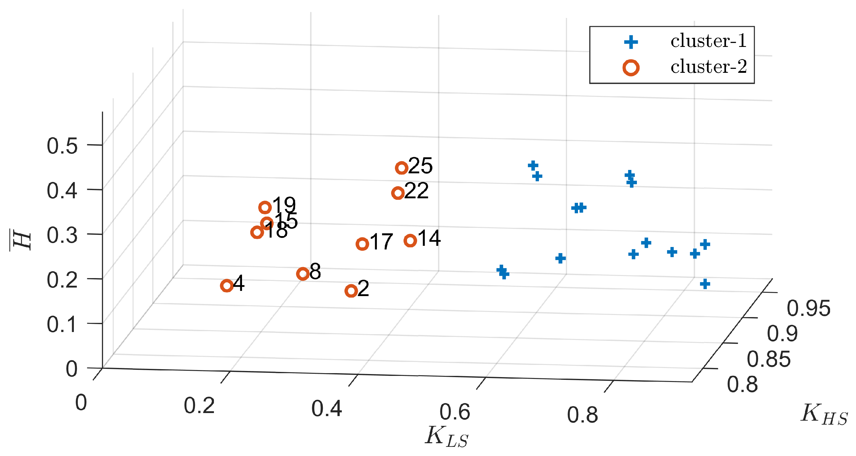
- It first defines and uses high-speed remaining torque and low-speed remaining torque as indicators to measure the similarity of rotor acceleration and deceleration processes. An adaptive K-means clustering method is introduced to identify sub-groups of induction motors, which facilitates a more reasonable reduction in the order of the dynamic model while ensuring the simplicity and usability of the load model.
- (2)
- It proposes using equal total power, equal total torque, and equal rotor stored kinetic energy as aggregation rules. An improved single-unit equivalent method for each induction motor sub-group is introduced, which enhances the accuracy of the reduced-order model and helps to prevent overly conservative or risky transient voltage stability simulation results.
- (3)
- Through transient voltage stability simulations in a typical distribution network, it is demonstrated that the induction motor model obtained using the proposed methods exhibits dynamic characteristics that are closer to those of the actual induction motor group compared to similar methods. Additionally, this confirms that the proposed methods more accurately reproduce the dynamic processes of transient voltage collapse.
2. Grouping and Aggregation Rules for Induction Motor Groups
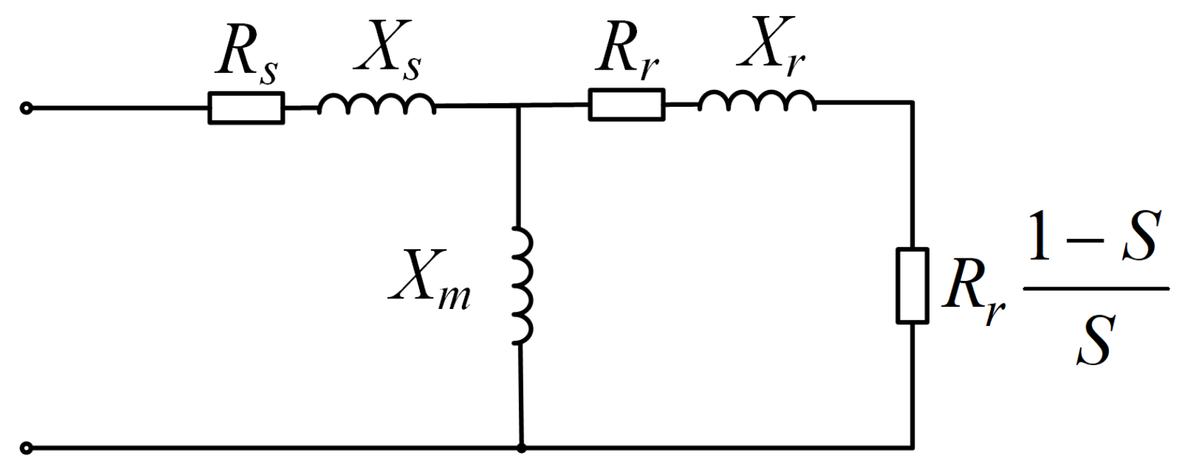
2.1. Model and Parameters of an Induction Motor
2.1.1. Parameters of an Induction Motor Model
2.1.2. Parameters of the Induction Motor Group
- (1)
- and ;
- (2)
- and its corresponding critical slip ratio ;
- (3)
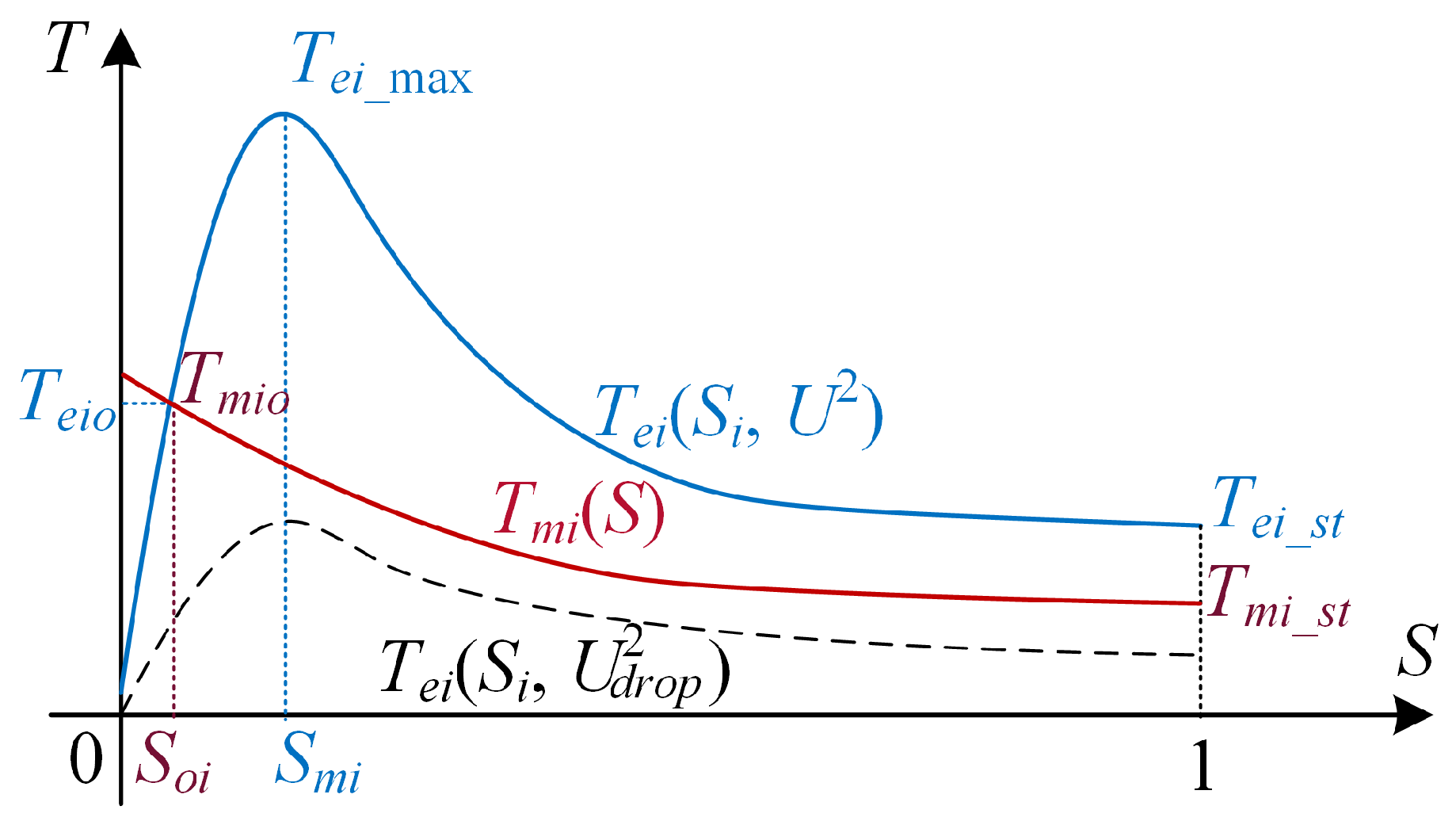
- The intersection of and within the interval . This intersection, where , represents the actual steady-state operating point for motor i.
2.2. Grouping Rules and Aggregation Rules
2.2.1. Rotor Motion Characteristics and Grouping Rules
2.2.2. Power Transmission Characteristics and Aggregation Rules
3. Grouping Method for the Induction Motors
3.1. Grouping Indicators
- (1)
- The internal factors determining the acceleration and deceleration rate of the motor rotor are its mechanical inertia and the resultant torque;
- (2)
- The external factors are the extent of the voltage drop and its duration.
- (1)
- Before the fault occurs in the power system, motor i operates normally with a constant speed. Therefore, in the interval , always holds true.
- (2)
- During a power system fault period, the voltage drops suddenly within a brief moment (less than 0.02 s). Therefore, in the interval , drops suddenly. As shown in Figure 2, the solid line drops to the dashed line . Since the mechanical torque depends on the resisting moment or inertia of mechanical load (such as pump or fan impeller) and cannot change suddenly, it can easily result in , causing the rotor to enter a braking and deceleration period. According to the equation, the greater the voltage drop and the smaller the moment of inertia , the faster the rotor decelerates. Conversely, the smaller the voltage drop and the greater the moment of inertia , the slower the rotor decelerates.
- (3)
- After the power system fault is cleared, the voltage gradually recovers, causing to rise gradually. In the interval , the relationship between and depends on the voltage change. According to the equation, the greater the voltage rise and the smaller the moment of inertia , the faster the rotor accelerates. Conversely, the smaller the voltage rise and the greater the moment of inertia , the slower the rotor accelerates.
3.2. Grouping Method Based on Adaptive K-Means Clustering
4. Aggregation Method for the Induction Motor Sub-Group
4.1. Calculation of Equivalent Impedance Parameters
4.2. Calculation of Equivalent Mechanical Parameters
5. Simulation and Discussion
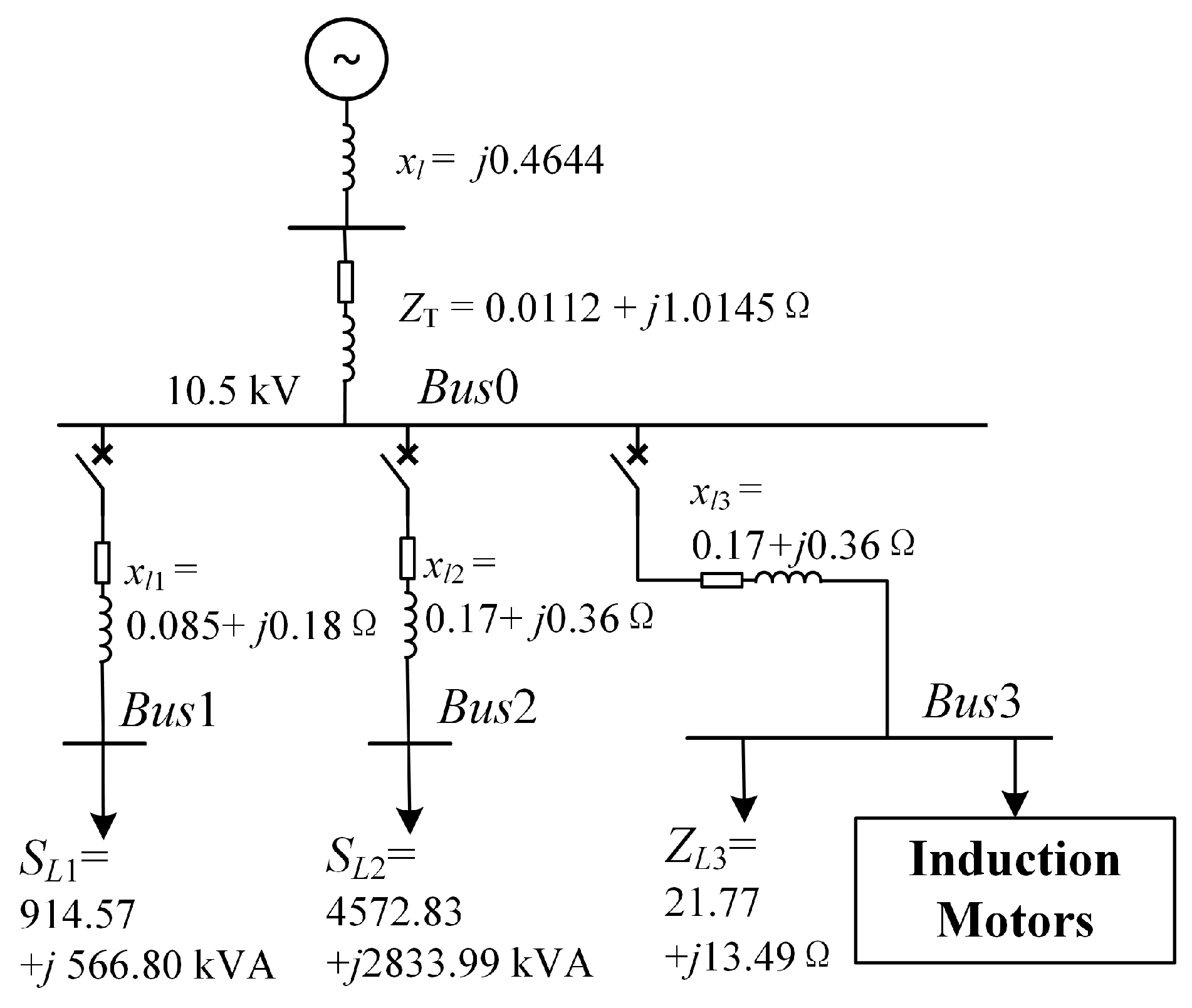
5.1. Simulation Setup
5.1.1. Distribution Network and Induction Motor Parameters
5.1.2. Simulation Arrangement
5.2. Simulation Results and Discussion
5.2.1. Grouping Results
5.2.2. Equivalent Results
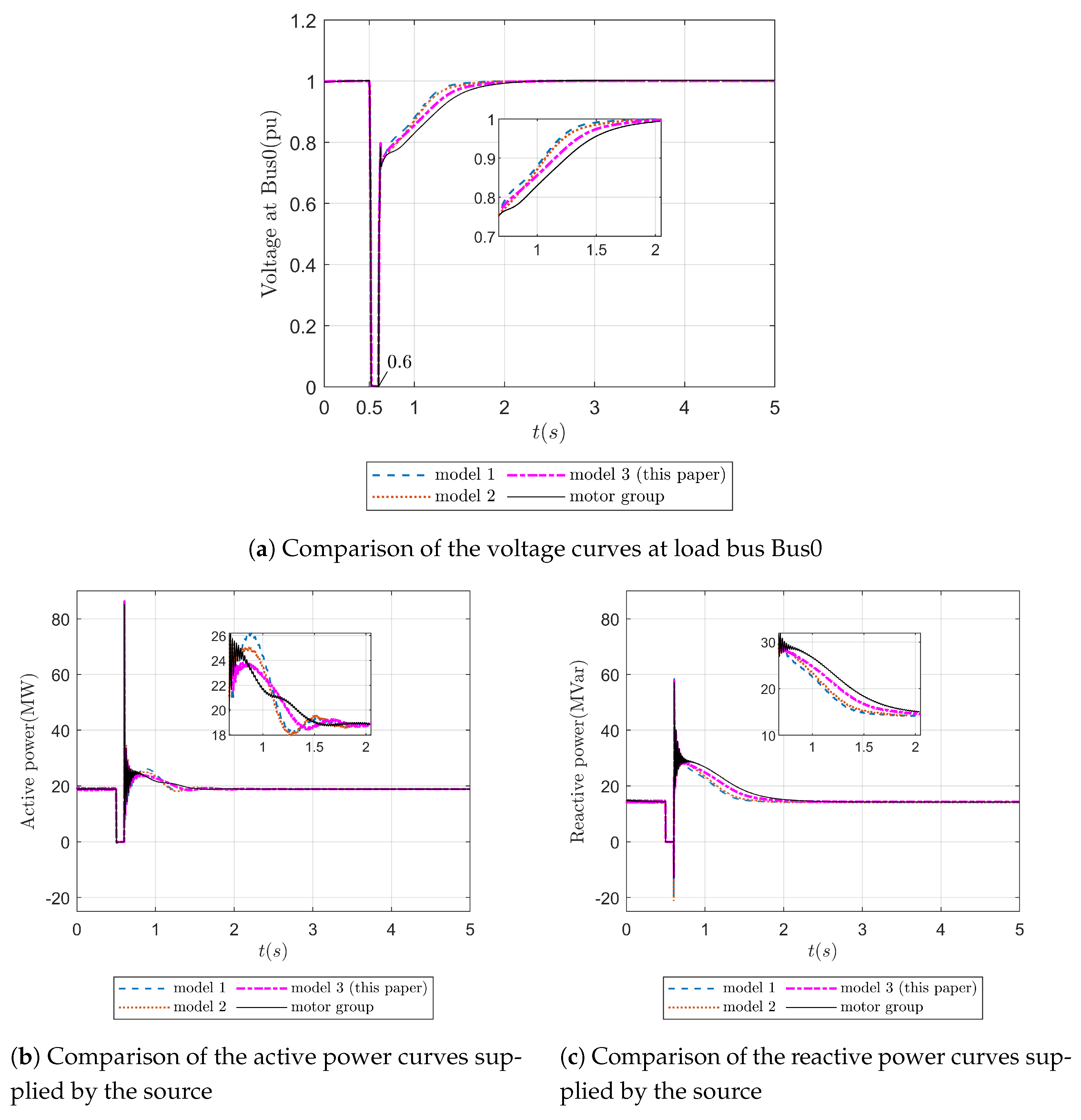
5.2.3. Transient Voltage Stability Results and Discussion
6. Conclusions
Author Contributions
Funding
Institutional Review Board Statement
Informed Consent Statement
Data Availability Statement
Conflicts of Interest
References
- Arif, A.; Wang, Z.; Wang, J.; Mather, B.; Bashualdo, H.; Zhao, D. Load Modeling—A Review. IEEE Trans. Smart Grid 2018, 9, 5986–5999. [Google Scholar] [CrossRef]
- Li, H.; Chen, Q.; Fu, C.; Yu, Z.; Shi, D.; Wang, Z. Bayesian Estimation on Load Model Coefficients of ZIP and Induction Motor Model. Energies 2019, 12, 547. [Google Scholar] [CrossRef]
- Kosterev, D.N.; Taylor, C.W.; Mittelstadt, W.A. Model Validation for the August 10, 1996 WSCC System Outage. IEEE Trans. Power Syst. 1999, 14, 967–979. [Google Scholar] [CrossRef]
- Pereira, L.; Kosterev, D.; Mackin, P.; Davies, D.; Undrill, J.; Zhu, W. An Interim Dynamic Induction Motor Model for Stability Studies in the WSCC. IEEE Trans. Power Syst. 2002, 17, 1108–1115. [Google Scholar] [CrossRef]
- IEEE Standards Association. IEEE Guide for Load Modeling and Simulations for Power Systems; The Institute of Electrical and Electronics Engineers, Inc.: New York, NY, USA, 2022. [Google Scholar]
- Cai, C.; Jiang, B.; Deng, L. General Dynamic Equivalent Modeling of Microgrid Based on Physical Background. Energies 2015, 8, 12929–12948. [Google Scholar] [CrossRef]
- Kundur, P.S.; Malik, O.P. Power System Stability and Control; McGraw-Hill Education: New York, NY, USA, 2022. [Google Scholar]
- Kryukov, A.; Suslov, K.; Ilyushin, P.; Akhmetshin, A. Parameter Identification of Asynchronous Load Nodes. Energies 2023, 16, 1893. [Google Scholar] [CrossRef]
- Kataoka, T.; Uchida, H.; Kai, T.; Funabashi, T. A Method for Aggregation of a Group of Induction Motor Loads. In Proceedings of the PowerCon 2000, 2000 International Conference on Power System Technology, Perth, WA, Australia, 4–7 December 2000; pp. 1683–1688. [Google Scholar]
- IEEE Task Force on Load Representation for Dynamic Performance. Bibliography on Load Models for Power Flow and Dynamic Performance Simulation. IEEE Trans. Power Syst. 1995, 10, 523–538. [Google Scholar] [CrossRef]
- Abdel Hakim, M.M.; Berg, G.J. Dynamic Single-Unit Representation of Induction Motor Groups. IEEE Trans. Power Appar. Syst. 1976, 95, 155–165. [Google Scholar] [CrossRef]
- Gentile, T.; Ihara, S.; Murdoch, A.; Simons, N. Determining Load Characteristics for Transient Performance. Volume 1: Executive Summary; EPRI: New York, NY, USA, 1981. [Google Scholar]
- Chen, M.S. Determining Load Characteristics for Transient Performances. Volume 3: Procedure for Modeling Power System Loads; EPRI: New York, NY, USA, 1979. [Google Scholar]
- Gentile, T.; Ihara, S.; Murdoch, A.; Simons, N. Determining Load Characteristics for Transient Performance. Volume 3: Load-Composition Data Analysis; EPRI: New York, NY, USA, 1981. [Google Scholar]
- Gentile, T.; Ihara, S.; Murdoch, A.; Simons, N. Determining Load Characteristics for Transient Performance. Volume 4: Test Results and Analysis; EPRI: New York, NY, USA, 1981. [Google Scholar]
- Electric Company General. Load Modeling for Power Flow and Transient Stability Computer Studies: Load-Modeling Reference Manual; EPRI: New York, NY, USA, 1987. [Google Scholar]
- Price, W.W.; Wirgau, K.A.; Murdoch, A.; Mitsche, J.V.; Vaahedi, E.; El-Kady, M. Load Modeling for Power Flow and Transient Stability Computer Studies. IEEE Trans. Power Syst. 1988, 3, 180–187. [Google Scholar] [CrossRef]
- Vaahedi, E.; Zein El-Din, H.M.; Price, W.W. Dynamic Load Modeling in Large Scale Stability Studies. IEEE Trans. Power Syst. 1988, 3, 1039–1045. [Google Scholar] [CrossRef]
- Franklin, D.C.; Morelato, A. Improving Dynamic Aggregation of Induction Motor Models. IEEE Trans. Power Syst. 1994, 9, 1934–1941. [Google Scholar] [CrossRef]
- Iliceto, F.; Capasso, A. Dynamic Equivalents of Asynchronous Motor Loads in System Stability Studies. IEEE Trans. Power Appar. Syst. 1974, PAS-93, 1650–1659. [Google Scholar] [CrossRef]
- Taleb, M.; Akbaba, M.; Abdullah, E.A. Aggregation of Induction Machines for Power System Dynamic Studies. IEEE Trans. Power Syst. 1994, 9, 2042–2048. [Google Scholar] [CrossRef]
- IEEE Task Force on Load Representation for Dynamic Performance. Standard Load Models for Power Flow and Dynamic Performance Simulation. IEEE Trans. Power Syst. 1995, 10, 1302–1313. [Google Scholar] [CrossRef]
- Du, W.; Su, G.; Wang, H.; Ji, Y. Dynamic Instability of a Power System Caused by Aggregation of Induction Motor Loads. IEEE Trans. Power Syst. 2019, 34, 4361–4369. [Google Scholar] [CrossRef]
- Ju, P.; Guo, D.; Cao, L.; Jin, Y.; Wang, Z.; Qian, C.; Wu, H. Review and Prospect of Modeling on Generalized Synthesis Electric Load Containing Active Loads. J. Hohai Univ. (Nat. Sci.) 2020, 48, 367–376. (In Chinese) [Google Scholar]
- Chen, Y.; Cheng, X.; Wu, H.; Shang, J. Aggregation of Induction Motor Group Considering Physical Characteristics and Static Critical Stable Characteristics. Power Syst. Technol. 2017, 41, 2964–2973. (In Chinese) [Google Scholar]
- Zhao, B.; Tang, Y.; Zhang, W. Study on Single-Unit Equivalent Algorithm of Induction Motor Group. Proc. CSEE 2009, 29, 43–49. (In Chinese) [Google Scholar]
- Hou, J.; Tang, Y.; Zhang, H.; Zhang, D. Study on Integration Method for Induction Motor. Power Syst. Technol. 2007, 4, 36–41. (In Chinese) [Google Scholar]
- Zhang, J.; Sun, Y.; Xu, J.; Liu, S. A Dynamic Aggregation Method for Induction Motors Based on Their Coherent Characteristics. Autom. Electr. Power Syst. 2010, 34, 48–52. (In Chinese) [Google Scholar] [CrossRef]
- Guo, J.; Yu, Y.; Li, P.; Zeng, Y. An Improved Weighting-Mean Aggregation Method of Induction Motors Considering Load Rates and Critical Slips. Autom. Electr. Power Syst. 2008, 14, 6–10. (In Chinese) [Google Scholar]
- Chen, Q.; Sun, J.; Cai, M.; Tang, Y. Parameters Determination of Synthesis Load Model Considering Distribution Network Connection. Proc. CSEE 2008, 16, 45–50. (In Chinese) [Google Scholar]
- Zhang, H.; Liu, Q.; Liu, Y. An Aggregation Method for Induction Motor Group and Its Testing with Dynamic Simulation. Power Syst. Technol. 2011, 35, 96–99. (In Chinese) [Google Scholar]
- Nozari, F.; Kankam, M.D.; Price, W.W. Aggregation of induction motors for transient stability load modeling. IEEE Trans. Power Syst. 1987, 2, 1096–1103. [Google Scholar] [CrossRef]
- Shi, G.; Liang, J.; Liu, X. Load clustering and synthetic modeling based on an improved fuzzy c means clustering algorithm. In Proceedings of the 2011 4th International Conference on Electric Utility Deregulation and Restructuring and Power Technologies (DRPT), Weihai, China, 6–9 July 2011; pp. 859–865. [Google Scholar]
- Ju, P.; Ma, D. Power System Load Modeling, 2nd ed.; China Electric Power Press: Beijing, China, 2008. (In Chinese) [Google Scholar]
- Tang, Y. Mathematical Models and Modeling Techniques for Power Load; Science Press: Beijing, China, 2012. (In Chinese) [Google Scholar]
- Cathey, J.J.; Cavin, R.K.; Ayoub, A.K. Transient load model of an induction motor. IEEE Trans. Power Appar. Syst. 1973, PAS-92, 1399–1406. [Google Scholar] [CrossRef]
- Zhang, J.; Zhang, C.; Yan, A.; Li, K. Aggregation method for multiple induction motors based on self-organizing neural networks and steady-state models. Autom. Electr. Power Syst. 2007, 31, 44–48, 86. (In Chinese) [Google Scholar]
- Lin, X.; Wu, H.; Liu, X.; Xu, B. Dynamic equivalent modeling of induction motors based on K-means clustering algorithm. In Proceedings of the 2019 IEEE PES GTD Grand International Conference and Exposition Asia (GTD Asia), Bangkok, Thailand, 19–23 March 2019; pp. 45–50. [Google Scholar]
- Zhang, S.; Chen, Y.; Yang, H.; Wu, H.; Ju, P. Comparison and analysis of grouping and aggregation algorithm for induction motor group. Energy Eng. 2024, 44, 117–126. (In Chinese) [Google Scholar]
- Shaw, S.R.; Leeb, S.B. Identification of induction motor parameters from transient stator current measurements. IEEE Trans. Ind. Electron. 1999, 46, 139–149. [Google Scholar] [CrossRef]
- Amaral, G.F.V.; Baccarini, J.M.R.; Coelho, F.C.R.; Rabelo, L.M. A high precision method for induction machine parameters estimation from manufacturer data. IEEE Trans. Energy Convers. 2020, 36, 1226–1233. [Google Scholar] [CrossRef]
- Tofighi, E.M.; Mahdizadeh, A.; Feyzi, M.R. Online estimation of induction motor parameters using a modified particle swarm optimization technique. In Proceedings of the IECON 2013—39th Annual Conference of the IEEE Industrial Electronics Society, Vienna, Austria, 10–13 November 2013; pp. 3645–3650. [Google Scholar]
- Louie, K.W.; Marti, J.R.; Dommel, H.W. Aggregation of induction motors in a power system based on some special operating conditions. In Proceedings of the 2007 Canadian Conference on Electrical and Computer Engineering, Vancouver, BC, Canada, 22–26 April 2007; pp. 1429–1432. [Google Scholar]
- Rousseeuw, P.J. Silhouettes: A graphical aid to the interpretation and validation of cluster analysis. J. Comput. Appl. Math. 1987, 20, 53–65. [Google Scholar] [CrossRef]
- Huang, K.; Tong, H.; Yang, J.; Li, H. Effects of leakage inductances on the dynamic characteristics and parameter identification of induction motor. J. Electr. Mach. Control 2002, 6, 179–181, 190. (In Chinese) [Google Scholar]
- Huang, K.; Liu, W.; Tong, H.; Yang, J.; Wu, Q. Accurate mathematical model and simulation for asynchronous motor. Electr. Mach. Control. Appl. 2001, 8, 17–19. (In Chinese) [Google Scholar]
- Zhao, B.; Tang, Y.; Zhang, W. Model representations of induction motor group in power system stability analysis. In Proceedings of the 2010 International Conference on Computer Application and System Modeling (ICCASM 2010), Taiyuan, China, 22–24 October 2010. [Google Scholar]


| Category | Details |
|---|---|
| Rated Parameters | Rated Voltage , Rated Power |
| T-Equivalent Circuit Parameters | |
| Rotor Parameters | Rotor Inertia and Time Constant |
| Mechanical Load Parameters | Mechanical Torque Coefficients |
| Category | Details |
|---|---|
| Starting Torque Parameters | Electromagnetic Torque , Mechanical Torque |
| Maximum Electromagnetic Torque Parameters | Critical Slip , Maximum Electromagnetic Torque |
| Steady-State Torque Parameters | Slip Rate , Electromagnetic Torque , Mechanical Torque |
| Steady-State Electrical Parameters | Stator and Rotor Currents and , Absorbed Active and Reactive Power , Electromagnetic Power |
| No. | (kW) | (kV) | Impedance (p.u.) | Mechanical Load | ||||||
|---|---|---|---|---|---|---|---|---|---|---|
| H (s) | (%) | a | ||||||||
| 1 | 1000 | 10 | 0.0379 | 0.1139 | 0.0079 | 0.1139 | 1.4411 | 0.6593 | 40 | 0.53 |
| 2 | 900 | 10 | 0.0176 | 0.122 | 0.0108 | 0.122 | 1.9507 | 0.7294 | 70 | 0.53 |
| 3 | 1000 | 10 | 0.0299 | 0.1172 | 0.0107 | 0.1172 | 1.6506 | 0.7706 | 50 | 0.53 |
| 4 | 2000 | 10 | 0.0351 | 0.1221 | 0.0086 | 0.1221 | 5.7783 | 0.8939 | 70 | 0.53 |
| 5 | 800 | 10 | 0.0159 | 0.123 | 0.0109 | 0.123 | 2.0896 | 0.9001 | 60 | 0.95 |
| 6 | 200 | 10 | 0.0129 | 0.1245 | 0.0109 | 0.1245 | 2.2618 | 0.9334 | 40 | 0.55 |
| 7 | 450 | 10 | 0.0485 | 0.0886 | 0.0116 | 0.0886 | 2.4915 | 1.1508 | 50 | 0.53 |
| 8 | 2000 | 10 | 0.0127 | 0.1281 | 0.0057 | 0.1281 | 3.7853 | 1.381 | 80 | 0.82 |
| 9 | 450 | 10 | 0.0728 | 0.0761 | 0.0173 | 0.0761 | 2.3504 | 1.4572 | 60 | 0.53 |
| 10 | 750 | 10 | 0.0334 | 0.0957 | 0.0117 | 0.0957 | 2.958 | 1.5721 | 70 | 0.87 |
| 11 | 900 | 10 | 0.0836 | 0.0634 | 0.0203 | 0.0634 | 1.9818 | 1.6141 | 60 | 0.53 |
| 12 | 450 | 10 | 0.0671 | 0.0793 | 0.0144 | 0.0793 | 2.4316 | 1.644 | 60 | 0.53 |
| 13 | 2000 | 10 | 0.0213 | 0.1251 | 0.0057 | 0.1251 | 3.5895 | 2.1137 | 40 | 0.82 |
| 14 | 750 | 10 | 0.0236 | 0.1231 | 0.0033 | 0.1231 | 2.9099 | 2.2128 | 80 | 0.95 |
| 15 | 750 | 10 | 0.0252 | 0.1226 | 0.0033 | 0.1226 | 2.8846 | 2.2852 | 70 | 0.87 |
| 16 | 1000 | 10 | 0.0232 | 0.1227 | 0.0111 | 0.1227 | 2.6789 | 2.3327 | 50 | 0.69 |
| 17 | 450 | 10 | 0.0218 | 0.1243 | 0.0034 | 0.1243 | 3.2272 | 2.3427 | 90 | 0.95 |
| 18 | 315 | 10 | 0.0231 | 0.1239 | 0.0056 | 0.1239 | 3.2025 | 2.532 | 90 | 0.82 |
| 19 | 750 | 10 | 0.0242 | 0.1229 | 0.0033 | 0.1229 | 2.9003 | 2.6363 | 70 | 0.87 |
| 20 | 1000 | 10 | 0.0239 | 0.1225 | 0.0111 | 0.1225 | 2.6691 | 2.7026 | 40 | 0.69 |
| 21 | 1000 | 10 | 0.0209 | 0.1235 | 0.0111 | 0.1235 | 2.712 | 2.8616 | 40 | 0.69 |
| 22 | 800 | 10 | 0.0099 | 0.1243 | 0.0032 | 0.1243 | 2.0193 | 3.1924 | 80 | 0.95 |
| 23 | 900 | 10 | 0.0123 | 0.123 | 0.0048 | 0.123 | 1.884 | 3.1972 | 60 | 0.9 |
| 24 | 900 | 10 | 0.0082 | 0.1242 | 0.0048 | 0.1242 | 1.9184 | 3.4254 | 60 | 0.9 |
| 25 | 800 | 10 | 0.0049 | 0.1258 | 0.0033 | 0.1258 | 2.0657 | 3.7413 | 80 | 0.95 |
| No. | Disturbance Settings | Induction Motor Model on Bus3 | |
|---|---|---|---|
| Model Description | Parameters | ||
| 1 | Disturbance 1: A temporary ground fault occurs on Bus0, lasting for 0.1 s. | Model 1: Single-unit model based on Ref. [32]. | See Section 5.2.2 |
| Model 2: Two-machine model based on Ref. [47]. | See Section 5.2.2 | ||
| Model 3: Models based on the proposed method in this paper. | See Section 5.2.2 | ||
| Motor Group: The actual group with 25 induction motors. | See Section 5.1.1 | ||
| 2 | Disturbance 2: A temporary ground fault occurs on Bus0, lasting for 0.2 s. | Model 1: Single-unit model based on Ref. [32]. | See Section 5.2.2 |
| Model 2: Two-machine model based on Ref. [47]. | See Section 5.2.2 | ||
| Model 3: Models based on the proposed method in this paper. | See Section 5.2.2 | ||
| Motor Group: The actual group with 25 induction motors. | See Section 5.1.1 | ||
| No. | (kW) | (kV) | Impedance (Ω) | Mechanical Load | ||||||
|---|---|---|---|---|---|---|---|---|---|---|
| H (s) | (%) | a | ||||||||
| C1 | 12,800 | 10 | 0.0346 | 0.1175 | 0.0111 | 0.1175 | 2.2653 | 1.9345 | 50.55 | 0.72 |
| C2 | 9515 | 10 | 0.0190 | 0.1327 | 0.0055 | 0.1327 | 3.0524 | 1.9084 | 76.18 | 0.79 |
| No. | (kW) | (kV) | Impedance (Ω) | Mechanical Load | ||||||
|---|---|---|---|---|---|---|---|---|---|---|
| H (s) | (%) | a | ||||||||
| 1 | 22,315 | 10 | 0.0300 | 0.1207 | 0.0093 | 0.1262 | 2.5387 | 1.9235 | 61.48 | 0.74 |
| No. | (kW) | (kV) | Impedance (Ω) | Mechanical Load | ||||||
|---|---|---|---|---|---|---|---|---|---|---|
| H (s) | (%) | a | ||||||||
| 1 | 20,515 | 10 | 0.0236 | 0.1205 | 0.0071 | 0.1205 | 2.5802 | 1.9534 | 61.61 | 0.77 |
| 2 | 1800 | 10 | 0.0784 | 0.0696 | 0.0182 | 0.0696 | 2.1665 | 1.5824 | 60.00 | 0.53 |
Disclaimer/Publisher’s Note: The statements, opinions and data contained in all publications are solely those of the individual author(s) and contributor(s) and not of MDPI and/or the editor(s). MDPI and/or the editor(s) disclaim responsibility for any injury to people or property resulting from any ideas, methods, instructions or products referred to in the content. |
© 2024 by the authors. Licensee MDPI, Basel, Switzerland. This article is an open access article distributed under the terms and conditions of the Creative Commons Attribution (CC BY) license (https://creativecommons.org/licenses/by/4.0/).
Share and Cite
Liang, Z.; Liu, Y.; Mo, L.; Zhang, Y. A Grouping and Aggregation Modeling Method of Induction Motors for Transient Voltage Stability Analysis. Energies 2024, 17, 4388. https://doi.org/10.3390/en17174388
Liang Z, Liu Y, Mo L, Zhang Y. A Grouping and Aggregation Modeling Method of Induction Motors for Transient Voltage Stability Analysis. Energies. 2024; 17(17):4388. https://doi.org/10.3390/en17174388
Chicago/Turabian StyleLiang, Zhaowen, Yongqiang Liu, Lili Mo, and Yan Zhang. 2024. "A Grouping and Aggregation Modeling Method of Induction Motors for Transient Voltage Stability Analysis" Energies 17, no. 17: 4388. https://doi.org/10.3390/en17174388
APA StyleLiang, Z., Liu, Y., Mo, L., & Zhang, Y. (2024). A Grouping and Aggregation Modeling Method of Induction Motors for Transient Voltage Stability Analysis. Energies, 17(17), 4388. https://doi.org/10.3390/en17174388