Review

A Comprehensive Review on Molecular Dynamics Simulations of Forced Convective Heat Transfer in Nanochannels

by
Rasoul Fallahzadeh
1,
Fabio Bozzoli
2,*,
Luca Cattani
2 and
Niloofar Naeimabadi
1
1
Department of Architecture and Engineering, University of Parma, 43124 Parma, Italy
2
Department of Engineering for Industrial Systems and Technologies, University of Parma, 43124 Parma, Italy
*
Author to whom correspondence should be addressed.
Energies 2024, 17(17), 4352; https://doi.org/10.3390/en17174352
Submission received: 2 August 2024 / Revised: 26 August 2024 / Accepted: 27 August 2024 / Published: 30 August 2024
(This article belongs to the Collection Advances in Heat Transfer Enhancement)

Abstract

:
As the demand for miniaturization of thermal management systems for electronic devices rises, numerous researchers are dedicating their efforts to the study of single-phase forced convective heat transfer (FCHT) within nanoscale channels. However, investigating FCHT in nanochannels (FCHT-NC) using experimental and theoretical methods is challenging. Alternately, molecular dynamics (MD) simulations have emerged as a unique and powerful technique in recent years. This paper presents a comprehensive review of the application of the MD simulation method in the study of FCHT-NC. Firstly, the current paper reviews various simulation techniques and models, along with their associated primary parameters employed in FCHT-NC, through a detailed and systematic literature survey and critical analysis. Evaluating the current methods and discussing their limitations provide helpful guidelines for future studies. Furthermore, based on the existing literature in the MD simulation, this review outlines all influencing parameters on the performance of FCHT-NC, covering their effects and discussing underlying mechanisms. Finally, key challenges and future research directions are summarized in this review, thereby providing essential support for researchers seeking to apply the MD simulation method to investigate FCHT-NC.

1. Introduction

In recent years, the investigation of flow properties within nanochannels (with the hydraulic diameter in the range of 0.1 to 10 μm [1]) has captured significant interest among scientists and researchers. Nanoflows have a wide range of applications, including fuel cells [2], drug delivery systems [3], and chemical measurement devices [4]. Furthermore, as modern electronic devices become increasingly thin, lightweight, and miniaturized, resulting in higher heat flux densities, new challenges arise regarding effective heat dissipation. Therefore, even though researchers have increasingly focused on various promising cooling techniques, such as jet impingement cooling [5,6,7,8] and spray cooling [9,10,11], single-phase forced convective heat transfer (FCHT) within nanoscale channels is also being investigated by many to develop highly reliable and safe thermal management systems. At the nanoscale, since the system spatial scale of the channels becomes comparable to the molecular mean free path of flowing fluid atoms, the nature of flow and FCHT exhibit distinct characteristics compared to the macroscale behavior [12]. Specifically, some interfacial phenomena that are usually neglected at the macroscale need to be reconsidered. In particular, the occurrence of a velocity jump in the nanochannel makes Navier–Stokes equations with the no-slip condition inapplicable [13]. The velocity jump is usually quantified using the slip velocity ( u s ) and the slip length ( l s ), which are schematically illustrated in Figure 1a. According to Navier’s model, u s , which is the difference between fluid velocity at the solid–fluid interface ( u y z = d ) and wall velocity ( u w = 0 ), is linearly proportional to the velocity gradient of the fluid at the solid–fluid interface ( u y z z = d ) [14]:
u s = u y z = d   u w = l s   ×   u y z z = d
As shown in Figure 1a, l s can be obtained by extrapolating the velocity profile from the solid–fluid interface to the position beyond the interface at which the fluid velocity is to be zero [15].
Moreover, thermal transport across the interface between the nanoflow and nanochannel walls leads to a temperature jump. In an analogous way to the (velocity) slip length, the temperature jump (Kapitza) length ( l k ) can be defined by extrapolating the fluid temperature profile from the solid–fluid interface to the position beyond the interface, where the temperature difference between the fluid and solid is zero, as shown in Figure 1b. l k could be defined as follows [16]:
l k = Δ T T z z = d
Δ T is the difference between fluid temperature at the solid–fluid interface ( T z = d ), and the wall temperature (Tw), and T z z = d is the temperature gradient of the fluid at the solid–fluid interface.
Although empirical and theoretical methods are frequently used to investigate FCHT at the macroscale, they encounter significant challenges when applied to nanochannel studies. Conducting experiments to study FCHT in nanochannels (FCHT-NC) presents numerous difficulties, including limitations of existing measuring technologies [17], their low accuracy [18], and high costs [19]. On the other hand, the reliability of theoretical approaches, which are based on significant assumptions, is also limited [20]. Therefore, due to its unique capability of providing fundamental insights at the nanoscale without continuum assumptions, the molecular dynamics (MD) simulation technique has emerged as a promising alternative method to study FCHT-NC. In the MD simulation of FCHT-NC, all the solid nanochannel wall and flowing fluid atoms are explicitly considered, and their detailed interactions are simulated. The FCHT behavior of the fluid in terms of its macroscopic properties is then investigated using appropriate statistical averages.
In 2005, Markvoort et al. [21] published the first paper on the MD simulation of FCHT-NC. They investigated the FCHT of a cold conceptual Lennard–Jones (CLJ) gas flowing through a hot CLJ nanochannel. By introducing the MD simulation technique for investigating FCHT-NC, they inspired many subsequent studies. The majority of the papers related to the MD simulation of FCHT-NC have been published within the last five years, indicating that the MD simulation of FCHT-NC is a new and developing research field. Even though leading expert researchers, such as Shuting Yao and co-authors [19,22,23,24,25,26,27,28], Zhao Song and co-authors [29,30,31], and Mohammad Bagheri Motlagh and co-authors [32,33,34,35], have conducted a series of important studies over the last decade, there is still a long way to go to obtain a comprehensive understanding of the underlying mechanics of the FCHT-NC and the influencing parameters. Furthermore, the MD simulation method still faces some unresolved issues that require adequate resolution.
Researchers have conducted a few review papers on the use of the MD simulation method in nanoscale heat transfer and thermofluidic sciences, which provide a wealth of useful information. Chatterjee et al. [36] conducted a review study on the application of MD simulations in nanoscale heat transfer. Their study covers topics such as evaporation at the liquid–vapor interface, the effects of pressure-varying fields on vaporization, and bubble dynamics at the solid–liquid–vapor interface. They also discuss theories of nanoscale heat transfer. Ran and Bertola [37] performed a comprehensive review on fluid flow and heat transfer issues at the nanoscale. Their study includes the physical modeling of heat transfer phenomena in MD simulations, covering areas such as boiling, evaporation, condensation, adiabatic processes, convective heat transfer flow, and two-phase flow in nanochannels. Compared with previous review works, however, this paper’s main contribution is its comprehensive yet concise overview of using the MD simulation method in FCHT-NC research.
As will be detailed in Section 2, researchers have utilized a diverse MD simulation method to explore the complex phenomena of FCHT-NC. These methods involve different models and techniques, each with its own set of advantages and limitations. A critical evaluation and comparison of these various approaches are crucial to assist researchers in identifying the most suitable simulation methods for their specific research objectives. By offering a comprehensive overview of the MD simulation techniques used in the study of FCHT-NC, this evaluation aims to provide researchers with a clearer understanding of how different methods can be applied and what outcomes they can expect. This guidance is intended to enhance the decision-making process when selecting simulation strategies, ultimately advancing research and innovation in the field of nanoscale thermal management.
Moreover, Section 3 will discuss the key factors that influence FCHT-NC. This section will focus on explaining how these factors affect the underlying mechanisms. It will also address inconsistencies reported in different studies. By examining these differences, the section aims to provide a clearer understanding of FCHT-NC. Additionally, it will suggest future research directions to explore, offering guidance on areas that need further study to resolve these discrepancies and enhance our comprehension of FCHT-NC. Therefore, by addressing the existing literature, this review offers a valuable resource for researchers to enhance their understanding of MD simulation in the context of FCHT-NC.
Nevertheless, this review paper has some limitations that should be acknowledged. Single-phase FCHT-NC involves the flowing fluid through a channel with a hydraulic diameter in the nanometer range and heat transfer resulting from the temperature difference between the nanochannel walls and the flowing fluid. Thus, this review does not cover MD simulation studies of adiabatic flowing fluids that only consider viscous dissipation (internal friction) as the heat source (see Refs. [38,39,40], for example), nor does it cover liquid-vapor phase transition heat transfer in flowing fluids (see Refs. [41,42], for example). Additionally, the present review does not include MD simulation studies of nano heat exchangers; however, their simulation principles are very similar to those of conventional nanochannels (refer to Refs. [43,44,45]). Still, this review remains a valuable resource for the MD simulation of adiabatic flowing fluids and nano heat exchangers.

2. Fundamentals of the MD Simulation Method in FCHT-NC

Classical MD simulation describes the interactions between atoms in a simulated system (simulation box) based on Newton’s laws of motion. Therefore, the system’s evolution can be examined from a dynamic perspective by simulating the movement of atoms over a desired time period. In recent decades, researchers have developed numerous techniques to improve the MD simulation method, some of which form the basis for the majority of MD simulation studies. Although many textbooks on MD simulations present the fundamentals of the MD simulation technique, this section provides a brief overview of the basic principles, focusing on their application in the study of FCHT-NC and highlighting the crucial steps and parameters. We encourage readers seeking a deeper understanding of the theory and implementation to consult the available textbooks [46,47,48]. As shown in Figure 2, the MD simulation of FCHT-NC generally follows five steps in the majority of MD simulation studies.
Step 1 (initial preparation) sets the foundation for the simulation by establishing the initial system conditions. This step includes selecting the nanochannel wall and fluid materials, constructing the initial simulation box, and determining the appropriate potential energy functions that will govern the interactions between the atoms. In step 2 (geometry optimization), the fabricated initial simulation box undergoes an energy minimization procedure to refine it into a more stable state. This step adjusts atomic positions to minimize the system’s potential energy, resulting in an optimized simulation box that serves as the basis for the next step. In step 3 (equilibrium MD (EMD) simulation), the optimized simulation box obtained from the previous step is allowed to evolve under controlled temperature and volume conditions until the system reaches thermal equilibrium. The outcome is an equilibrated simulation box that serves as a starting point for the next step. Step 4 (non-equilibrium MD (NEMD) simulation) then simulates FCHT-NC under a non-equilibrium condition. This step introduces a heat flux between the nanochannel walls and fluid domain while also establishing flowing fluid through the nanochannel. The non-equilibrium simulation captures the system’s dynamic behavior as it responds to these thermal and flow conditions, providing insights into FCHT mechanisms. Finally, the data obtained from the NEMD simulation in the previous step are extracted and interpreted in step 5 (data analysis). This step involves extracting meaningful information about various parameters and analyzing the results to draw conclusions. The following subsections provide further details about steps 1–4, while step 5 (data analysis) is discussed in the next section (Section 3).
It is worth noting that, as shown in Figure 2, both steps 3 (the EMD simulation) and 4 (the NEMD simulation) include a sub-stage named “solving Newton’s equations.” Given that the process of solving Newton’s equations is a general concept in all MD simulation methods, it is excluded here to maintain focus on MD simulations of FCHT-NC, and readers are encouraged to refer to existing textbooks [46,47,48] for further details.

2.1. Step 1: Initial Preparation

Before running an MD simulation, the first step is to select the nanochannel wall and fluid materials, construct the initial simulation box (including the definition of the shape and size of the simulation box, the initial position of atoms, and boundary conditions), and determine suitable potential energy functions.

2.1.1. Selection of Nanochannel Wall and Fluid Materials

In MD simulation studies focused on FCHT-NC, there are two types of atoms in the simulations: those comprising the flowing fluid domain and those comprising the solid nanochannel walls. Various materials have been considered in the current literature.
Argon (Ar), as a simple Lennard–Jones (LJ) fluid, is the most common flowing fluid in MD simulation studies of FCHT-NC, mainly because it has a simple atomic structure consisting of a single atom. This simplicity facilitates computational modeling and reduces the complexity of interatomic interactions compared to more complex materials [49]. Furthermore, Ar has well-understood thermodynamic properties, such as density, thermal conductivity, and shear viscosity, which allow researchers to validate their simulation methods by comparing their findings properties with experimentally established data, thereby making it a reliable fluid. Finally, the availability of numerous studies that use Ar as the flowing fluid in MD simulations of FCHT-NC provides an excellent opportunity to compare the obtained results with previous studies and to validate the simulation method. For example, Assadi et al. [35] compared their results with those of Tang et al. [50] to evaluate the accuracy of their simulation method.
Apart from Ar, some researchers have used water as the flowing fluid in their studies, mainly because of its relevance to real-world applications and, consequently, the ability to capture processes associated with real engineering nanochannels. The MD simulation method allows for the use of various water models (more than 40 distinct models [51]). Each water model makes slightly different assumptions regarding the effective charge magnitude on the hydrogen (H) and oxygen (O) atoms, the length of the H–O bonds, the H–O–H bond angle, and the use of additional mass-less sites, all of which result in different macroscopic thermophysical properties [52]. In the context of the MD simulation of FCHT-NC, three water models, including the SPC/E (extended simple point charge) [53], the TIP4P (transferable intermolecular potential with four points) [54], and the TIP4P/2005 (transferable intermolecular potential with four points developed in 2005) [55], are used as rigid molecules (with fixed bond lengths and bond angles). Figure 3 schematically depicts these models and their key parameters.
Even though all the mentioned water models offer a satisfactory balance of computational efficiency and accuracy, the TIP4P/2005 stands out as the most accurate one for calculating the density, thermal conductivity, and shear viscosity of water [64,65,66]. Nevertheless, none of these models accurately reproduce the thermophysical properties [67]. Consequently, for MD simulations of water flow in nanosystems, the five-site models, such as TIP5P-Ew [68], demonstrate significantly greater accuracy [67], thereby making them the preferred choice for future studies.
Several materials commonly serve as nanochannel walls in MD simulations of FCHT-NC. Copper (Cu) and platinum (Pt) are frequently used mainly due to their relevance to practical applications and simplicity. Among the studies referenced in this paper, only Marable et al. [61], Yu et al. [60], and Liu et al. [17] used double-layer graphene, silicon, and iron, respectively. Given the importance of silicon-based nanochannels [69], it is critical to promote the use of silicon as the nanochannel walls in MD simulations.
Some studies (for example, see Refs. [21,70]) use CLJ materials instead of real ones. The CLJ materials are considered to have a preferable atomic mass for an imaginary single-atom material that does not exist in the real world. However, the potential energy function describing the interactions between these atoms is defined based on the Lennard–Jones 12–6 (LJ 12–6) potential, which is described in Section 2.1.3. Since CLJ materials provide excellent flexibility in adjusting parameters, they allow for a better understanding of the underlying mechanisms of FCHT-NC. However, they cannot represent the complexities of real materials, especially compared to water molecules.

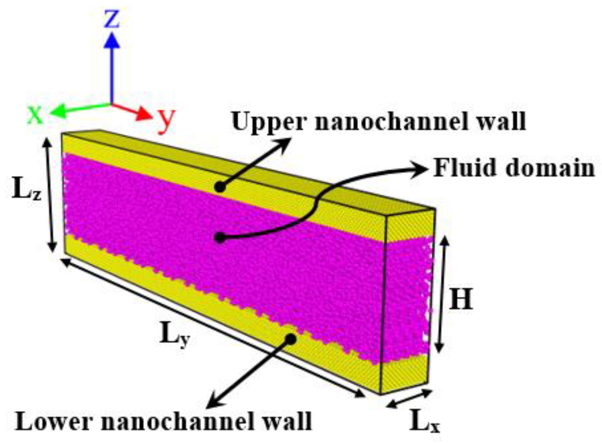
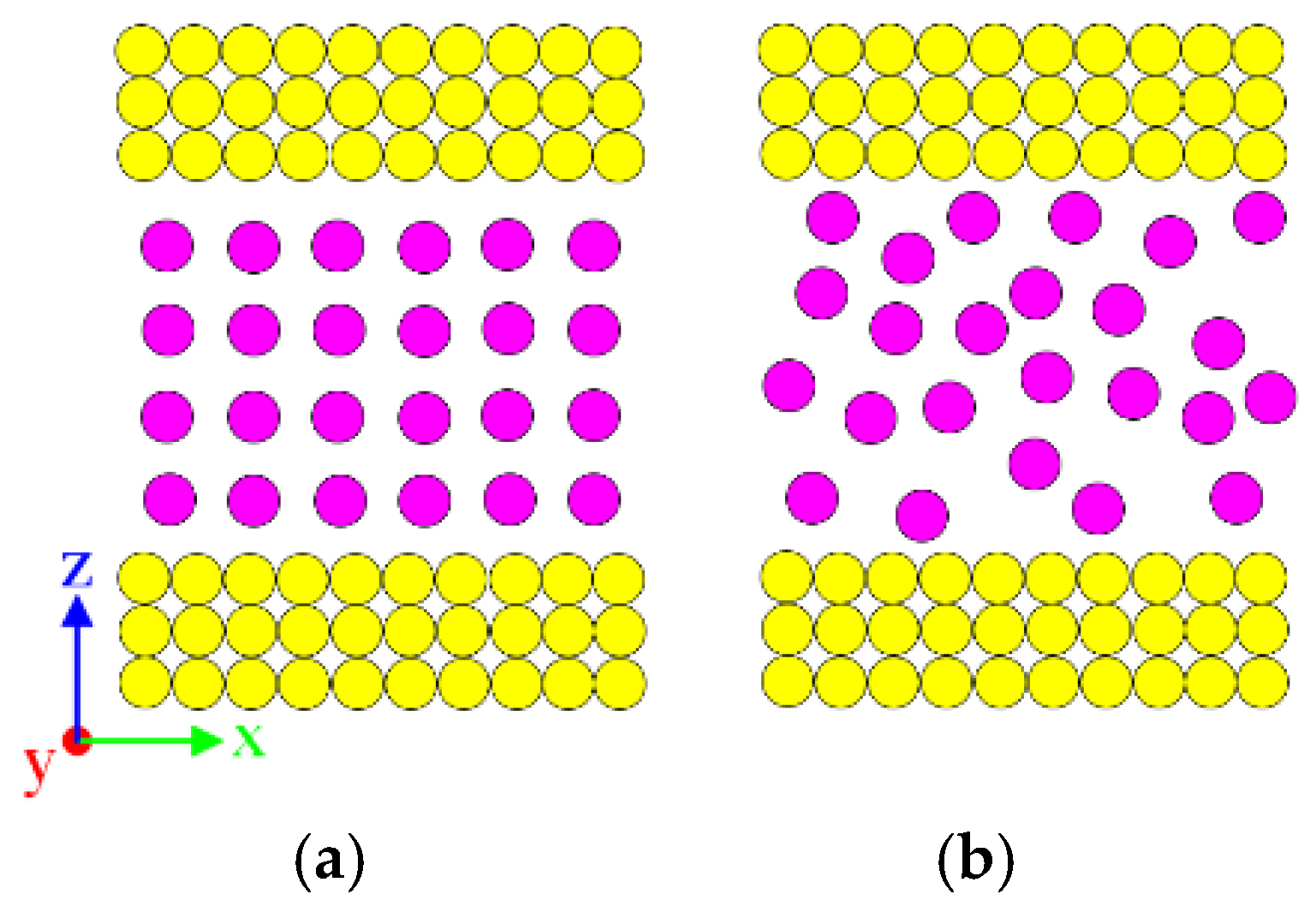
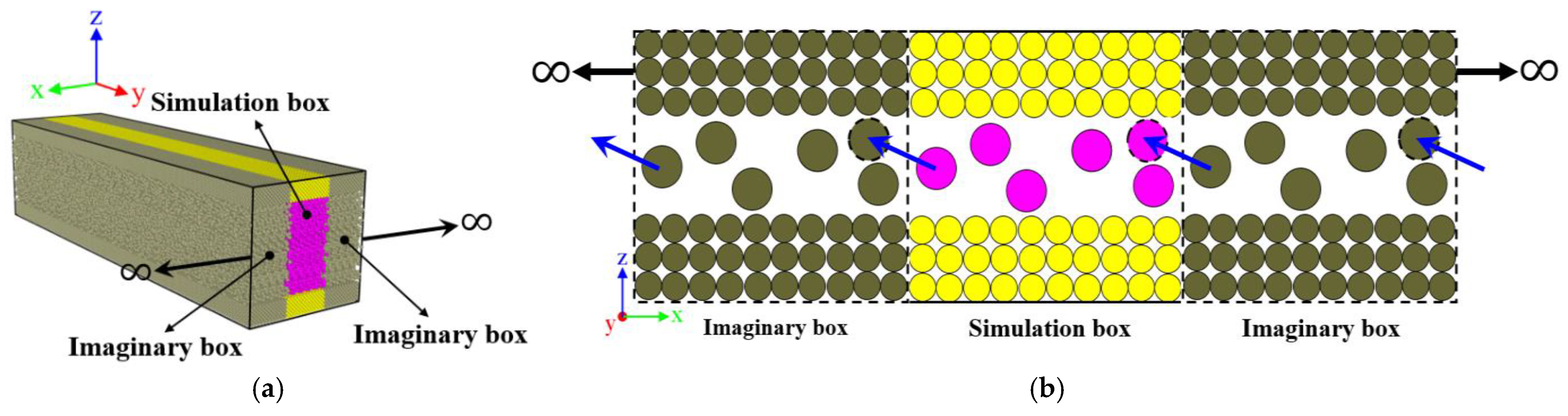
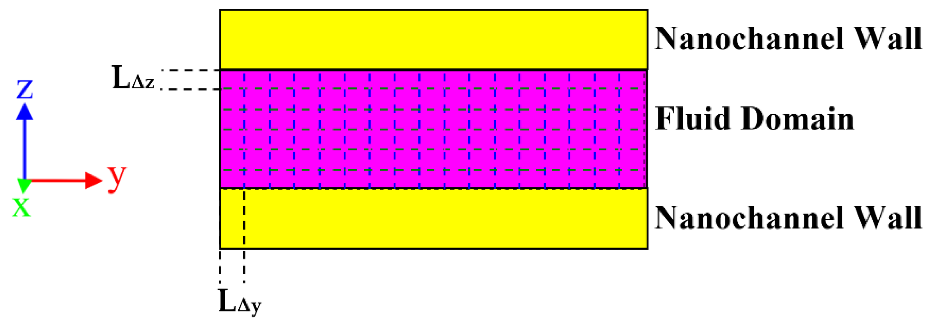
2.1.2. Construction of the Initial Simulation Box

It is essential to choose a suitable configuration of the simulation box, which allows the conduction of an in-depth investigation into FCHT-NC. Among the different five choices for the simulation box (see Ref. [71] for more details), the cubic shape is used in all studies due to its easy implementation and ability to mimic the actual shape of the nanochannels. Figure 4 displays a three-dimensional schematic of a conventional simulation box, consisting of two parallel solid walls located at a given distance from each other (called the channel height) in the bottom and top of the simulation box, and fluid particles (Ar atoms or water molecules) are placed in the space between the lower and upper nanochannel walls. This review paper designates the y-direction as the flow direction (the length of the simulation box) and the x-direction as the simulation box’s width, as shown in Figure 4. These definitions are maintained throughout the paper to ensure consistency.
For the simulation box, the literature uses various lengths (Ly), widths (Lx), and total heights (Lz = channel height (H) + solid wall thickness (d)). The inner surfaces of the upper and lower nanochannel walls are located at z = d and z = d + H, respectively. It is worth noting that these dimensions should meet some basic criteria. Usually, but not always, the Ly is chosen to be greater than the thermal entrance length (based on the Graetz number [72]) to ensure a fully developed laminar flow. The Lx should be large enough to meet the minimum image criterion (see Ref. [73] for definition and further details). Thus, it should exceed 2 r c [71] (where r c is the cut-off radius, further discussed in Section 2.1.3). More importantly, choosing much greater values ( 2 r c ) for the Lx does not influence the results, as shown by Marable et al. [61] and Ge et al. [74].
The upper and lower nanochannel walls are composed of solid atoms arranged in their predefined lattice structure. Each nanochannel wall may consist of one or several layers. Typically, researchers choose a wall thickness (d) larger than r c to eliminate its impact on solid-fluid interaction and, consequently, the FCHT-NC process. Therefore, most studies chose several layers of solid atoms (usually more than three layers) rather than a single layer. The outermost layer(s) of the upper and lower nanochannel walls, referred to as the fixed layer(s), is kept stationary at its initial positions to avoid wall deformation [27] and serve as an adiabatic boundary condition [33]. Most studies select a single solid layer as the fixed layer, which seems to work perfectly. However, Markvoort et al. [21] applied an alternative method to prevent solid wall deformation by resetting the total linear momentum of the nanochannel wall atoms to zero every several steps of simulation. Finally, the channel height (H) is one of the influencing parameters on the performance of FCHT-NC, which will be discussed in Section 3.3.6.
To define the fluid domain during the initial simulation box construction, one could either place the fluid particles based on an initially ordered structure or randomly distribute them, as shown in Figure 5.
The first method (ordered structure) is very popular and assumes a crystalline structure for the fluid domain, with the lattice constant value matching the fluid’s actual density. For example, Gonzalez and Law [49] set up the Ar atoms in a face-centered cubic (FCC) lattice corresponding to a density of 1200 kg/m3. In this scenario, fluid particles will move freely in the next steps of the simulation (throughout a so-called melting process of fluid [74]) and, subsequently, reach a thermodynamic equilibrium position. The fluid domain could be considered a liquid, gas, or supercritical fluid. Most studies adopted a supercritical fluid mainly because in this way, they can focus specifically on FCHT processes with no possibility of phase transition in the process [74].
In summary, an initial, finite-sized simulation box has been established up until now. Nevertheless, due to surface effects, atoms at the boundaries have fewer neighboring atoms compared to those within the simulation box. As a result, the dynamic behaviors of boundary atoms differ significantly from those inside the simulation box. Therefore, MD simulations apply periodic boundary conditions that allow for a small unit cell repeated in space, eliminating artificial surface effects and consequently mimicking an infinite system [75]. In the context of the MD simulation of FCHT-NC, periodic boundary conditions are imposed in the x- and y-directions by duplicating the initial simulation box periodically. As a result, atoms’ positions can vary within the range of −∞ < x < +∞ and −∞ < y < +∞. Figure 6a illustrates a schematic representation of duplicating the initial simulation box in the x-direction. As shown schematically in Figure 6b, when an atom exits the simulation box on one side, an equivalent image atom from an adjacent imaginary box enters the simulation box from the opposite side. Therefore, using periodic boundary conditions not only removes artificial surface effects but also maintains a constant number of particles within the simulation box, which is essential for MD simulations. However, as the real channel confines the fluid domain within the upper and lower nanochannel walls in the z-direction, the simulation box is subjected to fixed boundary conditions in this direction. It should be noted that two artificial pre-inlet regions are usually defined to create a Poiseuille flow and generate heat flux during the NEMD simulation step (Step 4), which will be discussed in Section 2.4. Therefore, the boundary condition in the y-direction in this step should be considered a quasi-periodic boundary condition. This condition is similar to the periodic boundary condition, with the difference that acceleration and temperature of the flowing fluid atoms would be reset before re-entering into the nanochannel.

2.1.3. Determination of Suitable Potential Energy Functions

Potential energy functions, which represent the interactions between atoms in the simulation box, are the most important aspect of MD simulations and must carefully be chosen to accurately describe the FCHT-NC. Generally, a single atom is influenced by the potential energy function of every atom in the simulation box, which can be divided into the atomic non-bonding interaction energy ( U non-bonded ) and the molecular internal bonding potential energy ( U bonded ); hence, the potential energy function can be defined as follows [76]:
U = U non-bonded + U bonded
As mentioned before, in the context of the MD simulation of FCHT-NC, solid and fluid materials are almost always either single atoms (such as Cu, Pt, and Ar) or rigid water molecules. Therefore, only atomic non-bonding interaction energies are considered, which are modeled as a sum of electrostatic ( U Elec ) and van der Waals ( U VW ) potentials as follows [76]:
U non-bonded ( r ij ) = U VW ( r ij ) + U Elec ( r ij )
Here, r ij represents the distance between two atoms. Moreover, common functional forms used to describe van der Waals and electrostatic interactions are the LJ 12–6 potential and Coulombic potential, respectively [77]:
U non-bonded ( r ij ) = 4 ε ij σ ij r ij 12 σ ij r ij 6 + q i q j 4 π ε 0 r ij
The first term on the right-hand side of Equation (5) represents the LJ 12–6 potential, in which σ ij (length parameter) is the distance where no interaction exists between two atoms and ε ij (energy parameter) is the depth of the potential well. The second term on the right-hand side of the equation represents the Coulombic potential, in which the charges of the i and j atoms are respectively defined by q i and q j , and ε 0 represents the dielectric constant. The choice of all the above-mentioned parameters is of crucial importance because they strongly influence the accuracy of the calculated thermodynamic properties. In the context of the interatomic interactions between solid-solid nanochannel wall atoms, which are modeled by the LJ 12–6 potential, the values of energy and length parameters for the common solid materials (Cu and Pt) are listed in Table 1.
However, it should be noted that pair potentials, such as LJ 12–6, cannot account for the strong bonding [79] and thermal motion [19] of solid atoms; therefore, usually a harmonic spring with a spring constant value (based on the Einstein crystal model [80]) is also added to create a simple harmonic vibration (see Refs. [74,81] for example). In this approach, a force of -Kr is applied to each solid atom at each step, where K is the spring constant and r is the atom’s displacement from its initial position to its current position. To achieve an accurate solid nanochannel wall, the correct spring constant must be used. The stiffness of the spring is related to Young’s modulus and can therefore be estimated accordingly [82]:
K = ED
Here, E stands for Young’s modulus, and D is the lattice constant of the metallic solid. Nevertheless, to overcome these difficulties, an alternative to the LJ 12–6 potentials, the embedded atom method (EAM) potential, has also been used as the more reliable potential to describe the interatomic interaction between solid-solid atoms. Under the embedded atom formalism, the total energy of atom i is expressed as [83]:
E total = F i ρ i + 1 2 i j φ ( r ij )
where F i represents the embedding energy of the i atom, ρ i expresses the background electron density at the i atom, and φ ( r ij ) represents the pair potential when two atoms are separated by the interatomic distance of r ij . However, using the EAM potentials may require significant computational resources, especially for a simulation box with a large number of solid atoms. Therefore, one could argue that since the main focus in the MD simulation studies of FCHT-NH is on heat transfer behaviors between the fluid domain and nanochannel walls as well as among the fluid domain and not on the solid nanochannel walls, the LJ 12–6 potentials, which require less computation cost than the EAM potentials [84], would be good enough [21]. However, studies have demonstrated that the LJ 12–6 potentials, when applied to a solid wall, fail to yield even approximately accurate surface energy values [85]. One alternative approach that could be considered for overcoming these obstacles is to use the LJ 12–6 potentials with parameters introduced by Heinz et al. [86]. They developed new parameters for metal materials, including Cu and Pt, that reproduce surface tensions and interface properties with water molecules comparable to the EAM potentials.
The LJ 12–6 potentials are also applied for the calculation of the fluid–fluid atom interactions. The energy and length parameters for the common fluid materials (Ar and water) are listed in Table 2. As can be seen in Table 2, to increase computational efficiency in the case of water, the LJ 12–6 potentials only count the interaction between O atoms, and LJ interactions between H atoms are not introduced, as these types of interactions are deemed negligible [61]. It should be noted that the potential function for water includes the contribution of electrostatic interactions, besides the LJ term.
The following modified LJ 12–6 potential, which is a combination of the potential models used by Din and Michaelides [87] and Barrat and Bocquet [88], is mostly used for the solid–fluid atoms interactions:
U sf ( r ij ) = 4 α ε sf σ sf r ij 12   β σ sf r ij 6
Here, s and f represent solid and fluid, respectively. Since solid and fluid refer to different types of atoms, the LJ parameters ( σ sf and ε sf ) for their interactions should be determined using a set of combining rules. Among the various combining rules, such as the geometric-mean rule [89,90] and the Waldman–Hagler rule [91], it is quite common to use the Lorentz–Berthelot (LB) rule [92], which uses a geometric mean for the length parameter ( σ sf ), Equation (9), and an arithmetic mean for the energy parameter ( ε sf ), Equation (10) [92]:
σ sf =   σ s + σ f 2
ε sf =   ε s   ε f
Moreover, in Equation (8), α and β are the potential energy factors indicating the strength of hydrophilic and hydrophobic interactions, respectively. The values of α and β can be set to different values to characterize different surface wettability. However, since the value of α has a bigger effect on changing the surface wettability than the value of β, all studies on the MD simulation of FCHT-NC considered β = 1 and only changed the value of α to obtain the desired wettability. As an alternative to Equation (10), some studies defined the ε sf based on the ε f , as follows:
ε sf =   χ ε f
Here, χ (usually called the scaling parameter) can be set to different values to obtain different surface wettability. Finally, in a quite rare method, Markvoort et al. [21] used the Weeks–Chandler–Andersen potential [93] to define different surface wettability. Unfortunately, after choosing and applying the solid-fluid LJ parameters ( σ sf and ε sf ), most studies did not calculate the contact angle of the fluid on the solid surface to support their predefined surface wettability. Among all related studies, Yao et al. [27,28], estimated the contact angle based on the droplet geometry method, which is not the best accurate technique (see Ref. [94] for more details).
As mentioned before, by duplicating the initial simulation box periodically, periodic boundary conditions are imposed in the x- and y-directions. A challenge posed by periodic boundary conditions is the increase in the number of interactions, making it impractical to calculate all of them in the MD simulation. Fortunately, most atomic interactions decay quickly with distance. Beyond a certain critical distance, known as the cut-off radius ( r c ), the interaction between two atoms becomes negligible and is typically disregarded in practical MD simulations. The usual values for r c have been chosen between 2.5 σ f and 4 σ f .

2.2. Step 2: Geometry Optimization

The goal of this step is to remove any steric clashes (due to the abnormal overlap of atoms) or poor geometric features from the initial simulation box and, consequently, find a stable starting simulation box with the least free energy and the greatest stability. Among different methods, such as steepest descent [95] and quasi-Newton [96] methods, energy minimization of the initial simulation boxes in the MD simulation of FCHT-NC is always performed by the conjugate gradient method, developed by Hestenes and Stiefel [97]. The simulation box obtained in this step (the optimized simulation box) is taken as the starting configuration for the next step.

2.3. Step 3: Equilibrium MD (EMD) Simulation

After completing the geometry optimization in the previous step, the MD simulation can finally be run. However, before performing an NEMD simulation to investigate FCHT-NH, an EMD simulation is conducted to achieve well-defined and uniform thermophysical properties. Prior to the EMD simulation, it is essential to define the initial ensemble and velocity.

2.3.1. Definition of Ensembles

Statistical mechanics introduced ensembles as concepts to more accurately characterize the behavior of a thermodynamic system. The simulation conditions determine the appropriate ensemble selection for a specific system (or one of its subsystems). A basic principle is that the chosen ensemble should ensure a representative sampling of the microscopic states to make accurate statistical arguments about the system. MD simulations can be carried out in different statistical ensembles, such as the microcanonical (NVE), canonical (NVT), isothermal-isobaric (NPT), isoenthalpic-isobaric (NPH), and grand canonical (μVT) ensembles. Generally, MD simulations of FCHT-NC are performed using the NVE and NVT ensembles. In the NVE ensemble, the number of atoms (N), system volume (V), and total energy (E) are kept constant. In the NVT ensemble, the number of atoms (N), system volume (V), and temperature (T) are kept constant.
During the EMD simulation step, usually an NVT ensemble is used for the entire simulation box, including the nanochannel walls and fluid domain, maintaining the temperature at a desired constant value. By maintaining a constant temperature, the NVT ensemble accurately reflects the canonical ensemble as described in statistical mechanics. This consistency ensures that simulation results are directly comparable to theoretical predictions and experimental data at specific temperatures. This is particularly important because in numerous experimental scenarios, systems are examined at constant temperature and volume, thereby making NVT simulations closely aligned with experimental conditions. To control the temperature, the simulation box is coupled with a so-called “thermostat,” which adjusts the energy within the system by either directly influencing the motion of atoms or altering their Newtonian equations of motion. Numerous thermostat algorithms are currently available to effectively control the temperature. A popular thermostat to control the temperature in the EMD simulation step is the Nose–Hoover thermostat [98]. The Nose–Hoover thermostat permits fluctuations in the total energy of a physical system while overcoming significant challenges associated with other thermostat methods. Unlike some alternative methods, it maintains a well-defined and conserved quantity, ensuring it represents a true canonical ensemble [99].

2.3.2. Definition of Initial Velocities

In theory, atoms can start with any arbitrary initial velocity. Over time, the simulation naturally adjusts these velocities to align with the assigned simulation conditions. To speed up the process, however, the initial velocities of the atoms are typically set according to the Maxwell–Boltzmann distribution [100], assigning velocities according to a distribution that matches the desired initial temperature.
There are many criteria to help determine when to stop the EMD simulation step, or, in other words, when the system has reached equilibrium. Generally, the most convenient method in MD simulation studies would be to plot the potential energy, total energy, and temperature as functions of time to check for equilibration and observe whether the simulation has reached relatively constant values with minor fluctuations. Unfortunately, almost all researchers did not report the aforementioned criteria.

2.4. Step 4: Non-Equilibrium MD (NEMD) Simulation

To study FCHT-NC, the MD simulation is continued from the equilibrated simulation box obtained from the previous step (the EMD simulation step). In this step, to simulate the heating or cooling of the flowing fluid, a flow and heat flux should be created, resulting in an NEMD simulation.

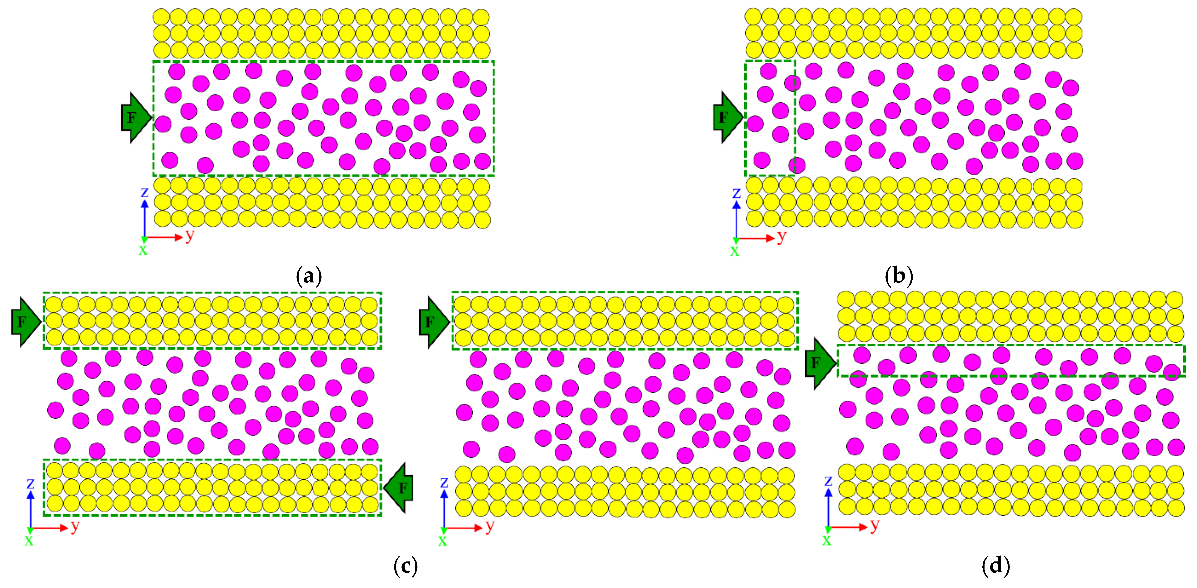
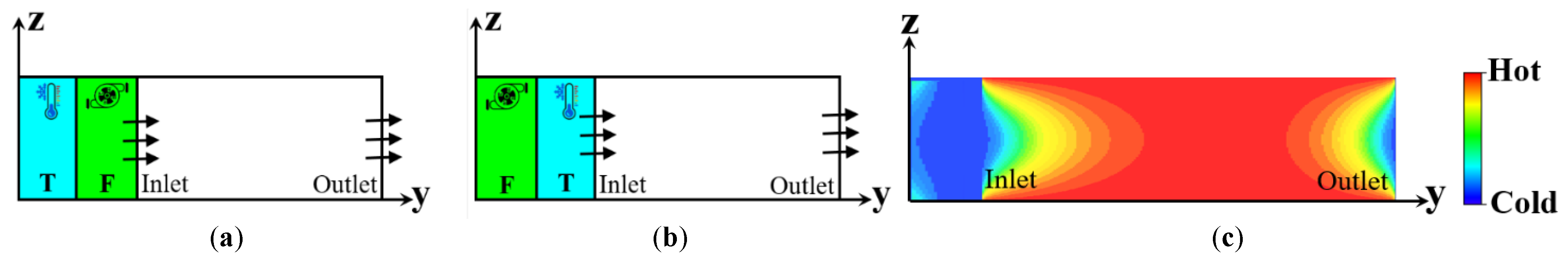
2.4.1. Flow Creation

Researchers investigating FCHT-NC have considered two primary flow models: Couette (shear-driven) flow and Poiseuille (force-driven) flow. Most studies focused on Poiseuille flow, with only a minority examining FCHT-NC under Couette flow. For the Poiseuille flow model, the fluid particles confined within the nanochannel walls are driven by an external force (F) exerted on the fluid atoms in the direction parallel to the nanochannel walls (in the y-direction). As schematically depicted in Figure 7a,b, there are generally two main models for creating Poiseuille flow: gravity-driven and pressure-driven models. In the gravity-driven model (Figure 7a), the external force is uniformly applied to each fluid atom; however, in the pressure-driven model (Figure 7b), the external force is applied only at a channel’s pre-inlet region (usually called the “forcing zone”), and the atoms in this region act as a fluidized piston that presses the rest of the fluid. It should be noted that in all studies concerning FCHT-NC, the influence of gravitational forces is typically excluded from MD simulations. This exclusion is due to the negligible impact gravity has on the relatively small number of atoms typically involved in such simulations. Therefore, the term “gravity-driven model” is used to describe this simulation approach not because actual gravitational forces are at play but because the method involves applying an external force (F) to each atom in a manner analogous to how gravity would act. Apart from Thekkethala and Sathian [20], almost all MD simulation studies of FCHT-NC with Poiseuille flow have adopted the pressure-driven model because the gravity-driven model added a significant amount of artificial energy to the simulation box [74].
For the Couette flow model, typically, the upper and lower nanochannel walls move in opposite directions to induce shear, or one wall remains stationary while the other moves (atomistic wall model), as schematically depicted in Figure 7c. However, Hu et al. [101] used an alternative model (the “fluid-like wall” model, based on the method introduced by Ashurst and Hoover [102]), where Couette flow is achieved with two stationary nanochannel walls and a moving fluid plate positioned beneath the upper nanochannel wall, as illustrated in Figure 7d. However, it should be mentioned that the atomistic wall model is more realistic than the fluid-like wall model [103]. Therefore, careful consideration is necessary regarding the implications of the fluid-like wall model, particularly in contexts where hydrophobic interactions between solid nanochannel wall and fluid atoms play a critical role. Given the critical role of nanostructured electrode materials in advanced electrochemical energy storage devices [104], investigating MD simulations of flow creation under the influence of external electric and magnetic fields—and studying their effect on TCHT-NC—would be an interesting research topic that has not yet been explored.

2.4.2. Heat Generation

As previously mentioned, during the EMD simulation, both the fluid domain and the nanochannel walls initially reach an equal temperature. To investigate FCHT-NC, however, a temperature gradient between the fluid domain and the nanochannel walls is required to induce heat flux. In this step, an NVE ensemble is first applied to the fluid domain without temperature control, allowing its temperature to develop naturally. Additionally, an NVT ensemble is used to maintain the nanochannel walls at a specific temperature.
To control the temperature of the nanochannel walls, two different models have been applied:
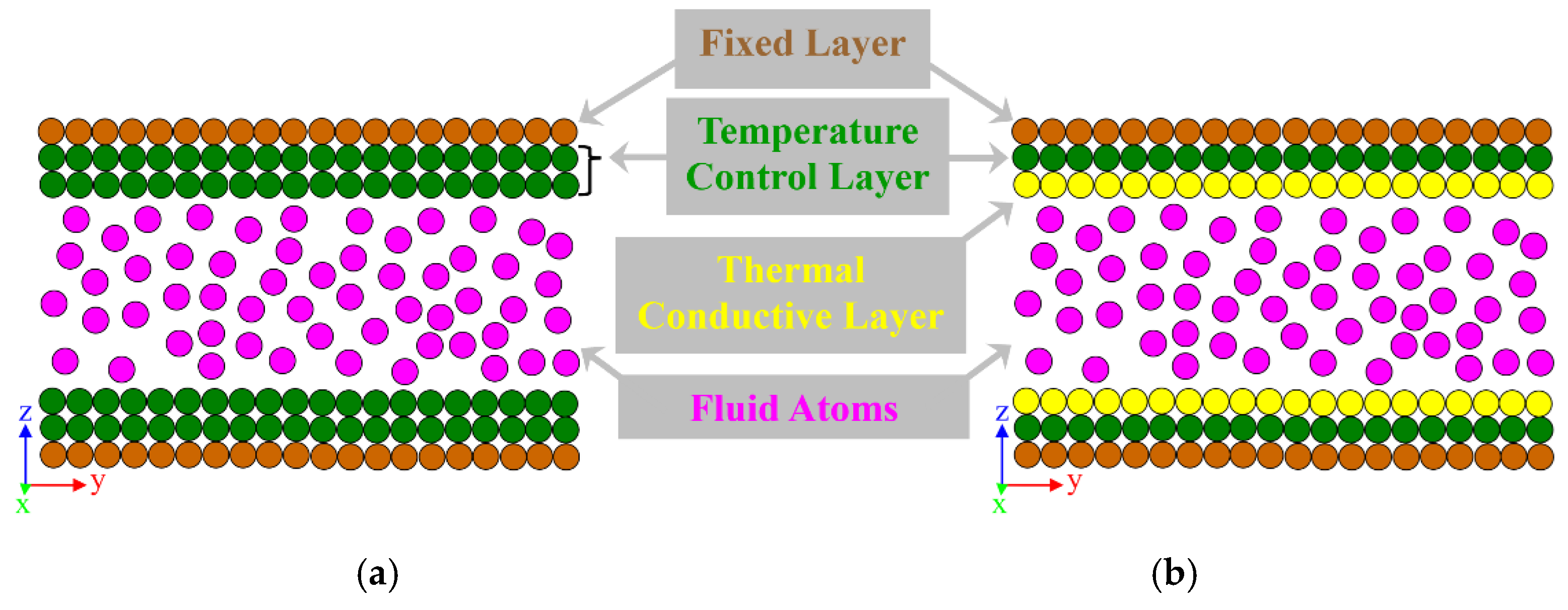
  • All-wall thermostat model (or cold-wall model): in this model, all nanochannel wall layers are selected as the region where the thermostat is applied to induce heat flux (see Figure 8a).
  • Partial-wall thermostat model (or thermal wall model): in this model, a small number of wall layers, called “temperature control layers,” which are sufficiently distant from the solid–fluid interface, are chosen as the region where a thermostat is applied. The next inner layers, called “thermal conductive layers,” interact freely with the neighboring atoms under an NVE ensemble (see Figure 8b).
It is important to note that for both models, the outermost layer of the upper and lower nanochannel walls (the fixed layer) is kept stationary to prevent wall deformation (as mentioned previously in Section 2.1.2). Although the partial-wall model is more common in MD simulation studies of liquid-vapor phase transitions on surfaces (see Refs. [105,106] for example), within the context of FCHT-NC, the all-wall thermostat model is typically used. However, since the thermostat controls the temperature based on the kinetic energy of atoms, leading to the application of a random force to maintain the prescribed temperature, the all-wall thermostat model can potentially cause an unphysical temperature jump at the solid–fluid interface. Consequently, this could result in an artificial solid–fluid interface resistance (refer to Ref. [107] for further details). Therefore, the partial-wall model is more suitable; and even though a few recent studies (Qin et al. [108], and Yao et al. [31]) applied that, it should receive more application.
To induce heat flux, in the case of a Couette flow model, different temperatures are applied to the upper and lower nanochannel walls (TUW ≠ TLW), as shown schematically in Figure 9a. However, in a Poiseuille flow model (Figure 9b), the majority of studies employed a symmetrical nanochannel wall temperature model, where both upper and lower nanochannel walls are at the same temperature (TUW = TLW), along with a temperature reset zone at the pre-inlet of the nanochannel with a different temperature (Tinlet ≠ TUW = TLW). Alternately, Qin et al. [108] employed an asymmetrical nanochannel wall temperature model, where the upper and lower nanochannel walls are at different temperatures (TUW ≠ TLW), along with a temperature at the reset zone that is equal to the upper nanochannel wall temperature (Tinlet = TUW).
In both symmetrical and asymmetrical nanochannel wall temperature models, in the temperature reset zone, the temperature of fluid atoms that are about to re-enter the simulation box (because of the periodic boundary condition in the y-direction) is reset to the desired inlet temperature (Tinlet). This reset is achieved by rescaling the velocity of every flowing fluid atom. Rescaling is performed by subtracting the local mean velocity, then changing the velocity to the desired inlet temperature, and finally adding back the local mean flow velocity that was initially removed. In the symmetrical nanochannel wall temperature model, depending on whether the nanochannel walls’ temperatures (TUW and TLW) are higher or lower than the inlet temperature (Tinlet), the simulation will represent a cold flow through a hot nanochannel (heating process) or a hot flow through a cold nanochannel (cooling process), respectively.
Popular thermostats to control the temperature of nanochannel walls (TUW and TLW) are the Langevin [109] and Nose–Hoover thermostats, while the most common thermostats to control the temperature of the fluid in the temperature reset zone domain (Tinlet) are Langevin, Nose–Hoover, and Berendsen [110] thermostats.
It should be noted that, as mentioned in Section 2.4.1, in the Poiseuille flow model, another pre-inlet zone (the forcing zone: to form a Poiseuille flow) has also been applied. Therefore, as shown in Figure 10, two different arrangements (named “thermal pump method”) for the forcing zone and temperature reset zone order can be applied. Markvoort et al. [21], who first introduced the thermal pump method, placed the forcing zone behind the temperature reset zone (as shown schematically in Figure 10a). However, this arrangement causes the inlet fluid’s temperature to be affected by the external force (which adds kinetic energy to flowing fluid atoms) and drift from the desired inlet temperature. Therefore, Ge et al. [74] slightly improved the arrangement by exchanging the order of the zones, as shown in Figure 10b. The Ge method has become the most common method used in MD simulations of FCHT-NC with the Poiseuille flow model and shows a well-controlled temperature of the inlet flowing fluid (see Refs. [27,33,74]). However, according to Thomas and Vinod [111], by using the Ge method, the inlet particles retain a memory of their preceding states, which subsequently modifies the initially uniform flow conditions at the inlet, especially during prolonged simulations. Moreover, the periodic boundary condition applied in the flow direction induces unrealistic axial heat conduction (as shown in Figure 10c), as reported by many studies such as Refs. [19,33,61]. This is due to the fact that the temperature of flowing fluid at the outlet is affected by the image atoms of the pre-inlet zones. Hence, typically only the data from almost the first half of the nanochannel are used for the analysis of FCHT-NC [74,81]. Even though it has been shown that in high Peclet (Pe) numbers (e.g., Pe > 10 [112,113] or Pe > 100 [114]), the axial heat conduction is negligible, improvements to the Ge thermal pump method are crucial for future studies.

3. Analysis of the MD Simulation of FCHT-NC

As soon as the fluid atoms exit the pre-inlet zones (the forcing and temperature reset zones), they enter the data collection zone, where the FCHT-NC simulation is conducted. To understand and quantitatively investigate FCHT-NC, researchers typically compute various parameters obtained from the NEMD simulation step, including the two-dimensional temperature distribution, local average fluid temperature, local Nusselt (Nu) number, radial distribution function (RDF), mean squared displacement (MSD), and vibrational density of states (VDOS). Given that RDF, MSD, and VDOS calculations are typical in MD simulations and are detailed in many textbooks (see Ref. [71], for example), they are not discussed here. The first subsection, however, provides the methodology for computing the two-dimensional temperature distribution, local average fluid temperature, and local Nu number. Following this, the typical performance of FCHT-NC, considering the most common simulated configuration (a cold Poiseuille flow through a hot nanochannel), is discussed. While other configurations could exhibit similar performance characteristics, they are not mentioned here to avoid lengthening this section, and readers are encouraged to consult the existing literature for further details. The final subsection discusses the parameters influencing the performance of FCHT-NC as reported by scholars.

3.1. Basic Governing Equations

To determine the distribution of different parameters of the fluid, the fluid domain is divided into Nx × Ny × Nz bins with dimensions of LΔx × LΔy × LΔz along the x-, y-, and z-directions, respectively. Figure 11 shows a schematic representation of divided fluid domain along the y- and z-directions. The number of bins in the x-, y-, and z-directions (Nx, Ny, and Nz, respectively) should be chosen carefully: LΔx, LΔy, and LΔz should not be too large to ensure that meaningful parameter variations are captured, nor too small to avoid the presence of empty bins without any data. Therefore, the sizes of bins are typically chosen to be on the order of σf.
Because there is flow in the nanochannel, the velocity of each fluid atom consists of both the mean flow velocity and the thermal velocity. Therefore, to calculate the average temperature in each bin for each time step, it is necessary to subtract the directional mean flow velocity ( u avg ) from the total atom velocity ( u i ) [32]:
T ( y , z ) = 1 3 Nk b i = 1 N m f u i   -   u avg 2
Here, k b is the Boltzmann constant, N is the number of fluid atoms, m f is the atom mass of fluid, and u i is the velocity of atom i.
To investigate the distinction of the fluid temperature over the cross-section along the flow direction at different positions, the local average fluid temperature ( T m ( y ) ) can be expressed as below [78]:
T m ( y ) = d d + H c p ρ y , z u y y , z T y , z dz d d + H c p ρ y , z u y y , z dz
Here, c p represents the isobaric specific heat capacity for the fluid, which is regarded as a constant value, ρ y , z denotes fluid density, and u y y , z stands for the fluid’s streamwise velocity.
In the process of FCHT, the Nu number is always an essential dimensionless parameter to show directly how good the heat transfer capability is. The local Nu number can be calculated from Equation (14) [115]:
Nu   ( y ) = h ( y ) D h λ
where the D h is the hydraulic diameter ( D h = 2H), λ represents the thermal conductivity of the fluid, and h ( y ) is the local heat transfer coefficient, which can be determined using Equation (15) [115]:
h   ( y ) = λ T m ( y )     T W T z z = d
Another method for calculating h   ( y ) , although not widely used, involves calculating the local heat flux across the nanochannel’s surfaces ( q ( y ) ) using the total energy [20] and then applying the following equation [35]:
h   ( y ) = q ( y ) T m ( y )     T W

3.2. Overall Heat Transfer Performance

Considering a cold Poiseuille flow through a hot nanochannel, Figure 12 schematically illustrates the fluid temperature distribution contour graph ( T ( y , z ) ) and the local average temperature along the flow direction ( T m ( y ) ) in the fluid domain along the flow direction.
The fluid temperature in the forcing zone is influenced by the applied external force and the fluid temperatures near the outlet of the simulation box and is generally not of primary interest. When the fluid enters the temperature reset zone, its temperature is reset to the desired inlet temperature ( T inlet ), which is nearly uniform. As the fluid leaves the pre-inlet zones, it is gradually heated by the hot nanochannel walls through convective heat transfer, causing the fluid temperature to increase gradually along the flow direction. The flow initially enters the thermal entrance region and eventually reaches the thermally fully developed region. To analyze FCHT-NC, researchers could examine both the thermal entrance region and the thermally fully developed region, often known as the data collection zone; however, they typically focus on the thermally fully developed region.
During the thermal entrance region, the fluid temperature ( T m ( y ) ) increases exponentially, similar to what occurs in conventional channels at the macroscale with a constant wall temperature. In the thermally fully developed region, the temperature profile satisfies the required conditions for thermally fully developed flow, i.e., [81],
y T W T ( y , z ) T W T m ( y ) = 0
Both the solid–fluid interface resistance (Kapitza resistance) and the boundary layer influence the local Nu number in the thermal entrance region. In scenarios where surface wettability is very low, Kapitza resistance becomes the dominant factor. Consequently, reducing temperature differences between the nanochannel wall and the flowing fluid along the y-direction leads to a decrease in Kapitza resistance and, thereby, an increase in the local Nu number at the thermal entrance region. Conversely, the boundary layer’s effect becomes more pronounced in very high surface wettability cases, and the local Nu number gradually decreases as the boundary layer develops along the y-direction [81].
Nevertheless, the local Nu number approaches a constant value in the thermally fully developed region. For macroscale FCHT, the fully developed Nu number for laminar flow between two parallel plates with constant wall temperature is 7.541 [74]. Depending on the Kapitza resistance, the Nu number of FCHT-NC could be lower or higher than that at the macroscale. Suppose the Kapitza resistance can be neglected. In that case, the Nu number gradually approaches 7.541, which is no different from that at the macroscale scale. Hence, the presence of the Kapitza resistance significantly affects FCHT-NC and is the primary reason why the Nu number at the nanoscale differs from that at the macroscale.
Finally, the fluid temperatures near the outlet decrease unrealistically due to the unrealistic axial heat conduction, as mentioned previously in Section 2.4.2.

3.3. Influencing Parameters on FCHT-NC

Conventional thermal management systems are struggling to meet the heat dissipation requirements of high-heat flux devices. Therefore, there is an urgent requirement to discover new methods to enhance the FCHT performance of nanochannels. This section details the various strategies proposed to improve the FCHT-NC performance in MD simulation studies. The main objective of this section is to address two issues. One is to uncover the impact of various parameters in FCHT-NC. The other is to enhance understanding of the underlying microscopic mechanisms influencing each parameter despite discrepancies between the findings of different MD simulation studies. Therefore, an introduction to the primary underlying microscopic mechanism governing FCHT-NC is discussed first. We will refer to the key concepts introduced here while reviewing the influencing parameters.
Based on the distance between the innermost solid nanochannel wall atoms and fluid atoms (rsf), we can divide the fluid domain into three different regions in the z-direction. As shown in Figure 13, the fluid atoms at the equilibrium distance (rsf = rmin) are defined as “the adsorbed film layer”. Any fluid atom with a distance less than rmin (rsf ˂ rmin) would be subjected to a strong repulsive force from the solid atoms. On the other hand, fluid atoms are subjected to a strong interaction force with solid atoms with a distance more than rmin (rsf ˃ rmin). However, as mentioned in Section 2.1.3, beyond the cut-off radius (rsf ˃ rcut), the solid–fluid interactions are considered negligible. We refer to the near-wall region as the area where the fluid atoms interact with the nanochannel walls (rmin ˂ rsf ˂ rcut). Moreover, the fluid domain beyond that (rsf ˃ rcut), where the fluid atoms could move freely without any interaction force from the solid nanochannel wall atoms, is called the mainstream region.
As can be seen in Figure 13, the total thermal resistance ( R total ) consists of the nanochannel wall conduction thermal resistance ( R s ), the Kapitza resistance at the solid-fluid interface ( R k ), and the fluid convection resistance in the near-wall and mainstream regions ( R f ). The influence of R s is not considered in the FCHT-NC simulations for two main reasons: (1) As outlined in Section 2.4.2, most MD simulation studies implement a thermostat across all nanochannel wall layers to induce heat flux, a model known as the all-wall thermostat approach. (2) Although metals’ total thermal conductivity comprises electronic and phonon contributions [116], the LJ 12–6 potential (the most used interatomic interactions between solid–solid nanochannel wall atoms) does not consider the presence of electrons [117] and exclusively addresses the phonon part of thermal conductivity. The R k in nanoscale heat transport depends strongly on thermal transport property differences between the solid nanochannel walls and fluid domain. Since the thermal transport properties of materials can fundamentally be determined based on their VDOS [118], the primary reason for R k is the different vibration frequencies of solid atoms in nanochannel walls and fluid atoms in the near-wall region. This frequency mismatch prevents efficient heat transfer across the solid–fluid interface.

3.3.1. Effect of Surface Wettability

When the characteristic size of the channel system is dramatically reduced to the nanoscale, the surface wettability significantly affects the FCHT performance and has been investigated by many researchers using the MD simulation method. In their studies, however, glaring inconsistencies in the classification of surface wettability could be found. As mentioned in Section 2.1.3, the surface wettability can be set at different values by tuning the energy parameter of the potential function between the solid–fluid atoms. In this review paper, therefore, the contact angle ( θ ) is calculated using Equation (18) [77]:
cos θ = 2 ε sf ε f   1
Subsequently, we utilized the definitions outlined by Peethan et al. [119] (Table 3) to categorize all the MD investigations concerning the impact of surface wettability in the FCHT-NC, as summarized in Table 4.
All studies on surface wettability have indicated a beneficial impact on improving FCHT as the surfaces become more hydrophilic. The analysis of the referenced studies to reveal the underlying mechanism, describing the positive effect of surface wettability, highlights one primary factor, known as the “(fluid) thermal bridge”, which is discussed in detail in the following.
When the solid–fluid interaction is strong enough, the average velocity of fluid atoms at the near-wall region decreases, making it difficult for most fluid atoms to flow. This immobilization causes the vibration frequency of the near-wall atoms to increase significantly, in contrast to the mainstream fluid atoms. While the vibration frequency of the near-wall atoms is higher than the mainstream atoms, it remains lower than the solid nanochannel wall atoms. Consequently, they could act as an overlapping region for thermal energy transmission from the solid nanochannel wall atoms to mainstream fluid atoms (like a thermal bridge). This phenomenon is particularly pronounced in situations involving high surface wettability. Hence, in high surface wettability conditions, the near-wall region atoms reduce interfacial thermal resistance, enabling more effective heat transfer. Furthermore, a low-potential energy region generally exists at the near-wall region due to the attraction between fluid and nanochannel wall atoms. As surface wettability increases, the attraction within the low-potential energy zone intensifies, effectively trapping more fluid atoms in the near-wall region. This results in a higher mass density of fluid at the near-wall region, which implies that more fluid atoms (per unit contact area) participate in heat transfer, reducing the Kapitza resistance and enhancing the overall heat transfer efficiency.
It is worth noting that the strong wall–fluid interaction inhibits the movement of fluid atoms, resulting in a decrease in fluid velocity in the near-wall and mainstream regions, and leading to an increase in fluid convection resistance. Generally, the reduction in the Kapitza resistance due to high wettability is a more significant factor than the increase in fluid convection resistance. However, as Yao et al. [19] demonstrated, if the solid–liquid interaction continues to increase beyond a critical value, the substantial rise in fluid convection resistance leads to very low fluid convection, ultimately decreasing the overall FCHT performance. Moreover, an interesting finding by Song et al. [31] is that a hydrophilic surface in FCHT-NC exerts a more significant positive influence than a non-smooth surface. Nonetheless, we will discuss in detail the impact of non-smooth surfaces on FCHT-NC later in this section.

3.3.2. Effect of Nanochannel Wall Material

Rather than artificially modifying surface wettability by manipulating solid–fluid atom interactions, as discussed in Section 3.3.1, an alternative and more realistic method involves altering the materials used as the solid nanochannel walls. However, the nanochannel wall materials must be selected by considering practical applications in the real world and computational feasibility. Because of the complexity of these considerations, MD simulation investigations into the impact of different nanochannel wall materials in FCHT-NC are relatively rare. In a notable study, Motlagh et al. [34] conducted an in-depth comparison of the effects of two nanochannel wall materials—Cu and Pt—on the performance of FCHT in a nanochannel filled with Ar. Their findings revealed that employing Cu instead of Pt could significantly enhance FCHT-NC. This improvement was primarily attributed to the stronger solid–fluid interactions between Cu and Ar atoms than between Pt and Ar atoms. The higher interaction strength increases heat transfer efficiency from the solid nanochannel walls to the fluid, as shown in the previous section (Section 3.3.1), enhancing FCHT-NC’s overall performance.

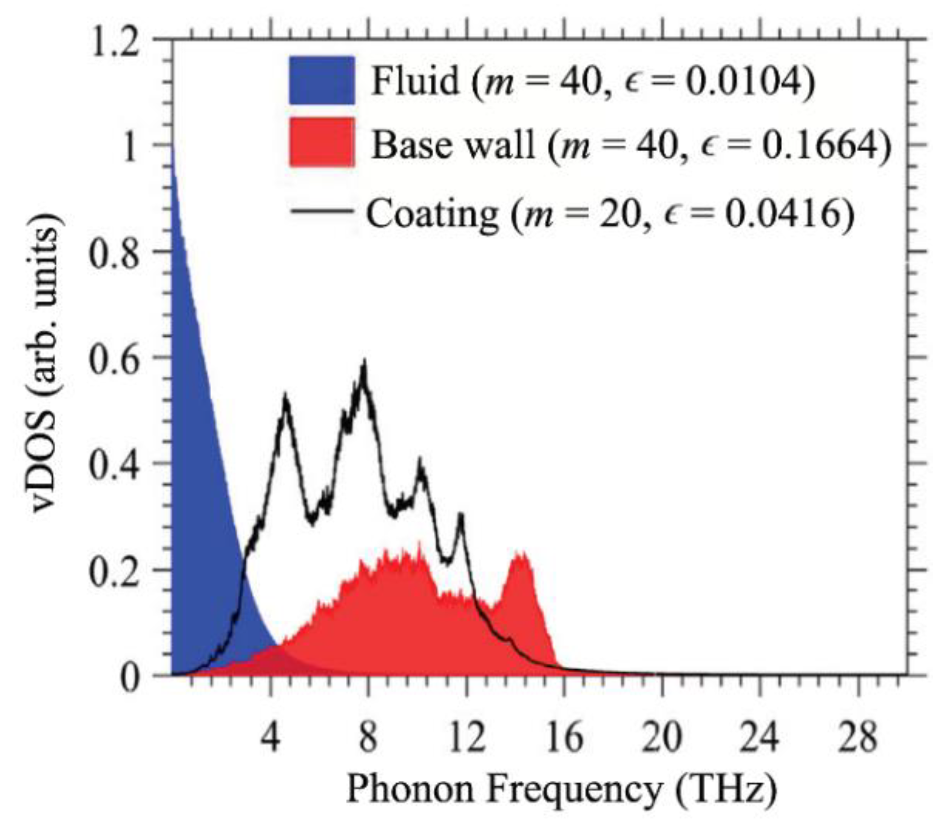
3.3.3. Effect of Surface Coating

Rather than either artificially modifying surface wettability by manipulating solid–fluid atom interactions or changing the nanochannel wall material, as discussed in previous sections (Section 3.3.1 and Section 3.3.2, respectively), a more practical approach is the deposition of coating materials. As summarized in Table 5, few MD simulation studies have investigated the impact of surface coating on FCHT-NC performance.
The deposition of coating materials changes the strength of solid–fluid atom interactions, influencing the vibrational mobility of the near-wall fluid atoms. As indicated in Section 3.3.1, the mismatch of vibrational properties between the solid nanochannel wall atoms and the near-wall fluid atoms plays a crucial role in Kapitza resistance. Therefore, if the VDOS of the coating material overlaps with the VDOS of both the solid nanochannel wall atoms and the near-wall fluid atoms, as shown in Figure 14, the coating layer acts as an excellent thermal bridge, thereby increasing the overall heat transfer between the nanochannel walls and fluid domain.
Otherwise, as shown by Thekkethala and Sathian [20], depositing a material that decreases the vibrational coupling between the solid nanochannel wall atoms and the near-wall fluid atoms, compared to uncoated nanochannel walls, leads to a remarkable decrease in heat transfer. Moreover, in this case, increasing the coating layer thickness could result in even lower heat transfer, mainly because of the reduced influence of the base nanochannel walls.
Interestingly, even after selecting the appropriate coating material, determining its optimal thickness remains crucial. MD simulation studies [23,70] have demonstrated a critical coating layer thickness beyond which the coating layer adversely affects heat transfer. Chakraborty et al. [70] hypothesized that this adverse effect arises from the conduction thermal resistance of a thick coating surpassing the thermal bridging effect, thereby decreasing the overall heat transfer. However, Yao et al. [23] showed that with an increase in coating thickness, the VDOS of the coating layer atoms initially increases the overlap area between the VDOS of the coating wall atoms and the near-wall fluid atoms and then gradually decreases. This results in an initial heat transfer enhancement and a subsequent decrease. As shown in Table 5, most molecular dynamics simulation studies on surface coating have utilized a CLJ material as the coating material. Nonetheless, it is vital to acknowledge the significance of more practical coating materials, including TiO2, SiO2/TiO2 bilayer, and SnO2/TiO2 bilayer [121], for more realistic applications in this context.

3.3.4. Effect of Surface Roughness

Due to technological constraints preventing the attainment of a perfectly smooth surface [78] and the proven benefits of nanostructured surfaces on FCHT-NC in experimental studies [122], many researchers (summarized in Table 6) have explored different surface roughness morphologies (schematically shown in Figure 15) to assess their impact on FCHT-NC.
These investigations consistently demonstrate that incorporating nanostructures onto ideally smooth surfaces substantially improves heat transfer efficiency as shown in Figure 16 for simple periodic sinusoidal nanostructured surfaces.
As previously mentioned, a low-potential energy region generally exists at the solid–liquid interface, attributable to the attraction between fluid atoms and the nanochannel wall atoms. Nanostructures, when introduced onto an ideally smooth surface, extend the low-potential energy region, thereby trapping and accumulating more atoms in the near-wall region. The increased concentration of fluid atoms intensifies the solid–liquid coupling, reducing Kapitza resistance and improving heat transfer. Moreover, Song et al. [30] postulated that surface roughness could intensify disturbances and enhance mixing in the near-wall region, consequently improving heat transfer efficiency. However, this hypothesis has been challenged by Chakraborty et al. [70].
To sum up, the main benefits of using nanostructured surfaces include increasing the contact area and their ability to trap fluid particles. Therefore, increasing the quantity of nanostructures by reducing their spacing can further enhance heat transfer efficiency. However, excessively minimizing the gaps between nanostructures may restrict the accessibility of fluid particles to the solid–fluid interface and diminish their beneficial impact (refer to Wang et al. [78] for further details). Furthermore, the heat transfer performance of the same nanostructure morphology, whether uniform or non-uniform, is almost identical as long as the contact areas they offer are the same (see Chakraborty et al. [70] for more information). Finally, using morphologies with enhanced fluid atom trapping capabilities results in much better FCHT performance. For instance, research by Chen and Li [115] suggests that utilizing rectangular nanostructures compared to triangular and hemispherical ones showed better heat transfer performance.
Most studies indicated that nanostructures hinder the movement of fluid atoms, resulting in reduced fluid velocity in both the near-wall and mainstream regions. This reduction leads to an increase in fluid convection resistance. In this context, the decreased Kapitza resistance, associated with the expanded heat transfer area, plays a more crucial role in overall heat transfer efficiency.
Contrary to expectations, MD simulations conducted by Motlagh and Kalteh [32,34] indicated that surface roughness does not necessarily reduce the fluid velocity. They postulated that using nanostructures in cavity forms instead of bumpy forms increased fluid velocity by expanding the space between the upper and lower nanochannel walls. On the other hand, Qin et al. [59] observed that employing nanostructures in bumpy forms instead of cavity forms, narrowing the cross-section, led to an increase in the fluid velocity. Despite these findings, other researchers have found that regardless of whether nanostructures are utilized as cavity forms or bumpy forms, they tend to decrease the fluid velocity.
Figure 15 clearly demonstrates the simplicity of all the nanostructures used in the FCHT-NC surface roughness investigation. However, perfect control over the shape and distribution of nanostructures is quite difficult; hence, using more complex morphologies (such as random surface roughness [125,126,127]) instead of these simple morphologies would be more realistic. Furthermore, since researchers have recently focused on using nanoporous materials to improve microchannel performance (refer to Refs. [128,129], for example), it would be intriguing to investigate their impact on the FCHT-NC system’s performance. There are several different MD simulation methods for the fabrication of metallic solid nanoporous materials (mostly used in the investigation of liquid-vapor phase transition on nanoporous surfaces) that could be applied (see Refs. [130,131,132,133], for example).

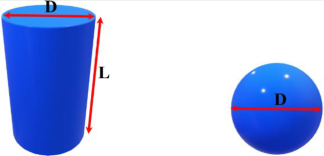
3.3.5. Effect of Adding Nanoparticles

It is well understood that the properties of the fluid domain significantly influence the efficiency of FCHT. One of the best ways to improve fluid properties is to suspend nanoparticles (ranging from 1 to 100 nanometers) into a base fluid, thereby creating what is known as a nanofluid [134]. Numerous studies have explored the impact of nanofluids on FCHT-NC performance in comparison to pure fluids, as summarized in Table 7. All studies have confirmed that adding nanoparticles to the base fluid enhances heat transfer, which aligns with experiments (for example, see Refs. [135,136]). MD simulations have aimed to uncover the underlying mechanism driving this enhancement to maximize this positive impact.
It is worth noting that when nanoparticles are introduced into nanochannels, they can be attracted to the nanochannel walls due to their strong interactions. As shown in Figure 17, we can identify two different states based on the predefined initial positions of the nanoparticles before the start of the MD simulations (during the construction of the initial simulation box). Initial placement of the nanoparticles in the upper and lower near-wall regions, close to the nanochannel walls, subjected them to a strong attraction from the solid nanochannel wall atoms, preventing them from freely moving with the base fluid atoms. This condition is known as the deposition state. Conversely, suppose we initially place the nanoparticles in the mainstream region, far beyond the direct interaction with the solid nanochannel wall atoms. In that case, the nanoparticles remain suspended and do not attach to the nanochannel walls. Since the nanoparticles in the nanochannel can exist in these two states—suspension and deposition—they play different roles in heat transfer. As a result, two mechanisms are responsible for improving FCHT-NC in the presence of nanoparticles. Before discussing the mechanisms, it is worth noting that deposited and suspended nanoparticles create a low-energy potential region around their surfaces due to stronger nanoparticle–fluid interactions than fluid–fluid ones. Consequently, they can easily attract fluid atoms at their interface and form a solid-like layer of fluid atoms around themselves, as shown in Figure 17. This solid-like layer plays a key role in increasing the FCHT, which is discussed in detail below.
The deposited nanoparticles act as nanostructured surfaces, decreasing the Kapitza resistance and consequently enhancing the FCHT (as mentioned in the previous subsection for the nanostructured surfaces (see Section 3.3.4)). Moreover, studies have shown that intense collisions of base fluid atoms with deposited nanoparticles in the near-wall region induce a spinning (rotational) motion of the deposited nanoparticles. This spinning motion mobilizes the solid-like layer atoms, accelerates the energy exchange, and improves heat transfer performance in the near-wall region.
However, this chaotic rotation motion is also reorganized for the suspended nanoparticles. Additionally, since the suspended nanoparticles can move freely in the mainstream region, they exhibit irregular Brownian (translational) motion in all directions within the nanochannel. The suspended nanoparticles’ random and chaotic motions disturb the flow domain and intensify collisions among fluid atoms, thereby improving the FCHT-NC.
Studies have shown that nanoparticle dimension, shape, and volume concentration can influence FCHT. As mentioned above, in the presence of nanoparticles, the solid-like layer is a critical factor in determining the performance of FCHT-NC. Increasing the nanoparticle diameter in the same volume concentration decreases their surface-to-volume ratio, reducing the number of solid-like layer atoms. This results in reducing the heat transfer capability of the nanofluid. Additionally, using cylindrical nanoparticles instead of spherical ones provides a higher surface-to-volume ratio, increasing the number of solid-like layer atoms, which is beneficial for heat transfer. Finally, increasing the volume concentration increases the number of solid-like layer atoms, which enhances heat transfer in the nanofluid. However, increasing the volume concentration decreases the distance between nanoparticles, potentially leading to nanoparticle aggregation, where nanoparticles attach to each other. Nanoparticle aggregation could result in a larger mass (consequently limiting their mobility) and a lower surface-to-volume ratio (consequently decreasing the number of solid-like layer atoms). Research indicates that the nanoparticle aggregation of Cu nanoparticles (compared to Pt nanoparticles) and cylindrical nanoparticles (compared to spherical nanoparticles) is notably rapid. Hence, careful consideration is essential when selecting nanoparticles.
In addition to the abovementioned reasons to explain the positive impact of adding nanoparticles on the FCHT performance, other possible reasons have been proposed in some studies, such as the higher thermal conductivity of metal nanoparticles (Cu and Pt) compared to the pure fluid (Ar) [33] and the acceleration of base fluid atom movement in the presence of nanoparticles compared to the pure fluid [32,33,123]. However, the former reason cannot be fully assessed in MD simulations, as simulations only address the phonon part of thermal conductivity of nanoparticles and not their electronic part. Also, the latter argument faced challenges from the findings of other studies (for example, refer to [49]).
The mentioned studies have primarily dealt with the addition of simple metal nanoparticles like Cu and Pt; it would be more practical to investigate the performance of commonly used and highly effective nanoparticles in nanochannel heat sinks such as SiO2 [138], CuO [139], TiO2 [140], and Al2O3 [141].

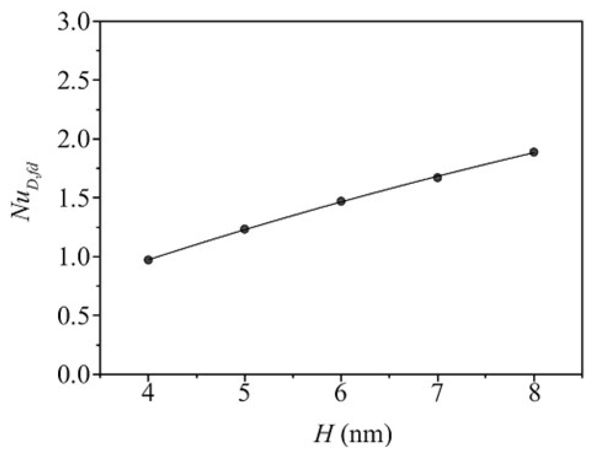
3.3.6. Effect of Channel Height

In MD studies, selecting an appropriate channel height is a critical task that balances computational feasibility with physical accuracy. In other words, excessively large channel heights are impractical because they require significant computational resources, making simulations time-consuming and costly. On the other hand, highly small channel heights fail to adequately represent the true bulk density of the fluid, leading to inaccurate simulations and unreliable results. Thus, researchers typically select channel heights within the range of four nanometers to several hundred nanometers to maintain this balance.
According to studies by Marable et al. [61] and Motlagh and Kalteh [34], increasing the channel height can significantly improve FCHT-NC, as shown in Figure 18.
The primary reason for this enhancement is the reduced impact of the Kapitza resistance as the channel height increases. In other words, when the channel height increases, the nanochannel wall atoms influence a smaller proportion of the fluid atoms. This reduction in the wall atom’s influence results in higher mobility of the fluid particles, improving heat transfer efficiency. In contrast, the studies by Ge et al. [74] and Gu et al. [112] have demonstrated different outcomes regarding the impact of increasing channel height on FCHT-NC performance. While Ge et al. [74] observed no significant effect, Gu et al. [112] reported a negative influence. Therefore, comprehending the impact of channel height on the FCHT-NC needs further exploration.

3.3.7. Effect of Fluid Velocity

Fluid velocity in a nanochannel can be controlled by varying the external force applied to the fluid atoms (in the Poiseuille flow model) or the nanochannel wall (in the Couette flow model). The fluid velocities achieved in MD simulation studies generally range from ~3 to ~300 m/s. According to MD studies by [60,61], increasing the flow velocity from relatively low to extremely high values does not significantly enhance FCHT-NC. In contrast, the studies by Thekkethala and Sathian [20] showed that increasing the fluid velocity has an adverse effect on the FCHT performance. They hypothesized that increasing the fluid velocity would shift the fluid particles out of the near-wall region. This causes a reduction in the vibrational mobility of the fluid atoms and reduces the heat transfer. However, experimental studies cannot support these findings (see Ref. [142], for example). Therefore, the precise understanding of the coupling effects of fluid velocity and FCHT efficiency in nanochannels is yet unclear and worthy of deep study.

3.3.8. Effect of Nanochannel Wall Temperature

Studies on the effect of nanochannel wall temperature on FCHT-NC are quite rare. This is primarily because researchers aiming to avoid phase change during simulations have not considered a wide range of nanochannel wall temperatures. Marable et al. [61] investigated the impact of varying the nanochannel wall temperature. As shown in Figure 19, their results indicated that increasing the graphene wall temperatures from 350 to 1000 K enhanced FCHT in the presence of water as the fluid domain. Higher wall temperatures increase the kinetic energy of fluid atoms, which leads to more collisions in the mainstream region and improves heat transfer.

4. Conclusions: Challenges and Future Directions

In light of the challenges in conducting experimental and theoretical studies, the MD simulations have emerged as an important alternative way to study FCHT-NC. In this review, we analyzed and discussed the methodologies, outcomes, and interpretations of studies employing MD simulations in the context of FCHT-NC. After conducting a brief analysis of the current state of various MD simulation models used by researchers to simulate the FCHT-NC, we identified several challenges that require further attention in future simulations, which are as follows:
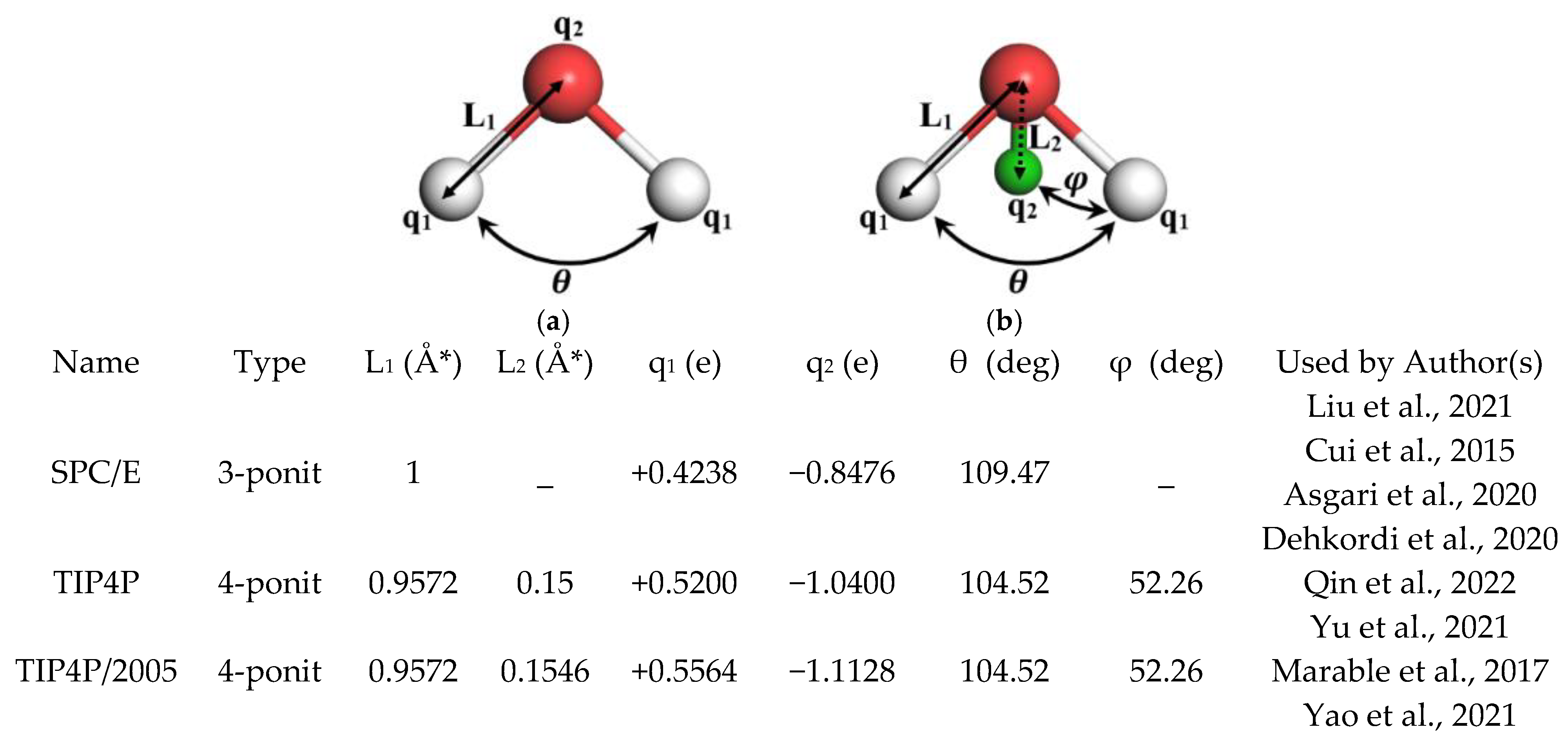
  • While various water models such as SPC/E, TIP4P, and TIP4P/2005 are typically utilized to simulate the fluid domain, five-site water models like TIP5P-Ew are anticipated to provide more accurate representations for future research.
  • Although Cu and Pt are frequently used as nanochannel wall materials mainly due to being practically applicable and simple, silicon, as a more commonly used material in practical applications, should receive greater attention.
  • Generally, researchers apply the LJ 12–6 and EAM potentials to represent the interactions between solid-solid nanochannel wall atoms. On one hand, the common length and energy parameters in the LJ 12–6 potential for metallic solid wall materials cannot account for the strong bonding and thermal motion of metallic solid atoms. On the other hand, using the EAM potentials may require significant computational resources. Meanwhile, Heinz et al. [65] introduced parameters for the LJ 12–6 potentials, which would be effectively employable and an excellent alternative.
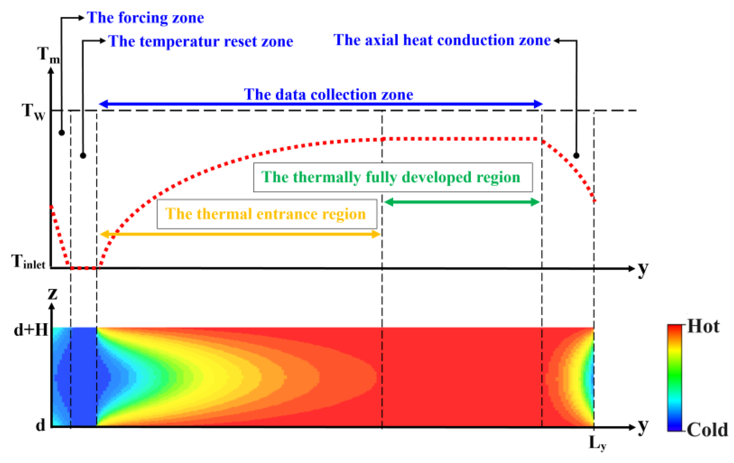
  • In MD simulations of FCHT-NC using the Poiseuille flow model, two distinct arrangements for the forcing zone and temperature reset zone order, referred to as the “thermal pump method”, have been implemented: the Markvoort method and the Ge method. Although the Ge method has become the most common and demonstrates effective control of the inlet fluid temperature, it results in unrealistic axial heat conduction. Consequently, improvements to the Ge thermal pump method are essential for future studies.
We then reviewed the underlying microscopic mechanisms influenced by various parameters, despite discrepancies between the findings of different MD simulation studies. We considered a variety of influencing parameters, including surface wettability, nanochannel wall material, surface coating, surface roughness, nanoparticle addition, channel height, fluid velocity, and nanochannel wall temperature. We have made recommendations for future research, which are as follows:
  • More studies are required to gain a comprehensive understanding of the complex relationship between the flowing fluid velocity and FCHT, particularly on nanostructured surfaces.
  • Using more complex morphologies (such as random surface roughness [116,117,118]) instead of these simple morphologies would be more realistic. Furthermore, since researchers have recently focused on using nanoporous materials to improve microchannel performance (refer to Refs. [119,120], for example), it would be intriguing to investigate their impact on the FCHT-NC system’s performance.
  • Recent studies indicate that adding nanoparticles into base fluids significantly improves the heat transfer efficiency. Future research should be carried out to explore commonly used nanoparticles like SiO2, CuO, TiO2, and Al2O3 for an optimal heat transfer performance.
  • Some research shows that raising the channel height can improve FCHT performance by lowering the Kapitza resistance. Others, however, show no significant effect or even negative impact. Therefore, conducting more research is necessary to comprehend the connection between the channel height and the FCHT efficiency.
  • The fluid velocity in nanochannels can be regulated by external forces, with MD simulations showing speeds of ~3 to ~300 m/s. While some studies suggest that higher velocities do not enhance the FCHT-NC performance and may even hinder it, experimental evidence does not support these claims. Therefore, the relationship between fluid velocity and the FCHT efficiency in nanochannels remains uncertain and requires more study.
By overcoming these challenges, we can enhance the capabilities of the MD simulation method in studying FCHT-NC and contribute to the advancement of nanochannels that exhibit an improved thermal performance.

Author Contributions

Writing—original draft preparation, R.F. and F.B.; writing—review and editing, L.C. and N.N.; supervision, F.B. All authors have read and agreed to the published version of the manuscript.

Funding

Niloofar Naeimabadi has a PhD fellowship in the framework of PR FSE 2021/2027 CUP D92J23000420006 (SOSTENIBILITÀ E RESILIENZA DELLA SOCIETÀ, DELLE CO-MUNITÀ E DEI TERRITORI), funded by EMILIA ROMAGNA REGION, Italy.

Conflicts of Interest

The authors declare no conflicts of interest.

References

  1. Zhang, X.; Ji, Z.; Wang, J.; Lv, X. Research progress on structural optimization design of microchannel heat sinks applied to electronic devices. Appl. Therm. Eng. 2023, 235, 121294. [Google Scholar] [CrossRef]
  2. Jana, K.K.; Srivastava, A.; Parkash, O.; Avasthi, D.K.; Rana, D.; Shahi, V.K.; Maiti, P. Nanoclay and swift heavy ions induced piezoelectric and conducting nanochannel based polymeric membrane for fuel cell. J. Power Sources 2016, 301, 338–347. [Google Scholar] [CrossRef]
  3. Bigham, A.; Hassanzadeh-Tabrizi, S.A.; Rafienia, M.; Salehi, H. Ordered mesoporous magnesium silicate with uniform nanochannels as a drug delivery system: The effect of calcination temperature on drug delivery rate. Ceram. Int. 2016, 42, 17185–17191. [Google Scholar] [CrossRef]
  4. Akbari, O.A.; Saghafian, M.; Shirani, E. Investigating the effect of obstacle presence on argon fluid flow characteristics in rough nanochannels using molecular dynamics method. J. Mol. Liq. 2023, 386, 122462. [Google Scholar] [CrossRef]
  5. Atofarati, E.O.; Sharifpur, M.; Meyer, J.P. Pulsating nanofluid-jet impingement cooling and its hydrodynamic effects on heat transfer. Int. J. Therm. Sci. 2024, 198, 108874. [Google Scholar] [CrossRef]
  6. Selimefendigil, F.; Ghachem, K.; Albalawi, H.; Alshammari, B.M.; Labidi, T.; Kolsi, L. Effects of using magnetic field and double jet impingement for cooling of a hot oscillating object. Case Stud. Therm. Eng. 2024, 60, 104791. [Google Scholar] [CrossRef]
  7. Forster, M.; Ligrani, P.; Weigand, B.; Poser, R. Experimental and numerical investigation of jet impingement cooling onto a rib roughened concave internal passage for leading edge cooling of a gas turbine blade. Int. J. Heat Mass Transf. 2024, 227, 125572. [Google Scholar] [CrossRef]
  8. Selimefendigil, F.; Benabdallah, F.; Ghachem, K.; Albalawi, H.; Alshammari, B.M.; Kolsi, L. Effects of using sinusoidal porous object (SPO) and perforated porous object (PPO) on the cooling performance of nano-enhanced multiple slot jet impingement for a conductive panel system. Propuls. Power Res. 2024, 13, 166–177. [Google Scholar] [CrossRef]
  9. Tian, J.; Li, B.; Wang, J.; Chen, B.; Zhou, Z.; Wang, H. Transient analysis of cryogenic cooling performance for high-power semiconductor lasers using flash-evaporation spray. Int. J. Heat Mass Transf. 2022, 195, 123216. [Google Scholar] [CrossRef]
  10. Tian, J.; He, C.; Chen, Y.; Wang, Z.; Zuo, Z.; Wang, J.; Chen, B.; Xiong, J. Experimental study on combined heat transfer enhancement due to macro-structured surface and electric field during electrospray cooling. Int. J. Heat Mass Transf. 2024, 220, 125015. [Google Scholar] [CrossRef]
  11. Qenawy, M.; Wang, J.; Tian, J.; Li, B.; Chen, B. Investigation of unsteady flow behavior of cryogen-spray coupled with cold air jet. Appl. Therm. Eng. 2023, 235, 121406. [Google Scholar] [CrossRef]
  12. Karimipour, A.; D’Orazio, A.; Shadloo, M.S. The effects of different nano particles of Al2O3 and Ag on the MHD nano fluid flow and heat transfer in a microchannel including slip velocity and temperature jump. Phys. Rev. E 2017, 86, 146–153. [Google Scholar] [CrossRef]
  13. Okechi, N.F. Stokes slip flow in a rough curved microchannel with transversely corrugated walls. Chin. J. Phys. 2022, 78, 495–510. [Google Scholar] [CrossRef]
  14. Nagayama, G.; Matsumoto, T.; Fukushima, K.; Tsuruta, T. Scale effect of slip boundary condition at solid-liquid interface. Sci. Rep. 2017, 7, 43125. [Google Scholar] [CrossRef]
  15. Dey, R.; Das, T.; Chakraborty, S. Frictional and heat transfer characteristics of single-phase microchannel liquid flows. Heat Transf. Eng. 2011, 33, 425–446. [Google Scholar] [CrossRef]
  16. Roy, P.; Anand, N.K.; Banerjee, D. Liquid slip and heat transfer in rotating rectangular microchannels. Int. J. Heat Mass Transf. 2013, 62, 184–199. [Google Scholar] [CrossRef]
  17. Liu, Y.; Liu, L.; Zhou, W.; Wei, J.A. Study of convective heat transfer by using the hybrid MD-FVM method. J. Mol. Liq. 2021, 340, 117178. [Google Scholar] [CrossRef]
  18. Kandlikar, S.G. Boiling and evaporation in microchannels. In Encyclopedia of Microfluidics and Nanofluidics, 1st ed.; Li, D., Ed.; Springer Science & Business Media: New York, NY, USA, 2008; pp. 158–159. [Google Scholar]
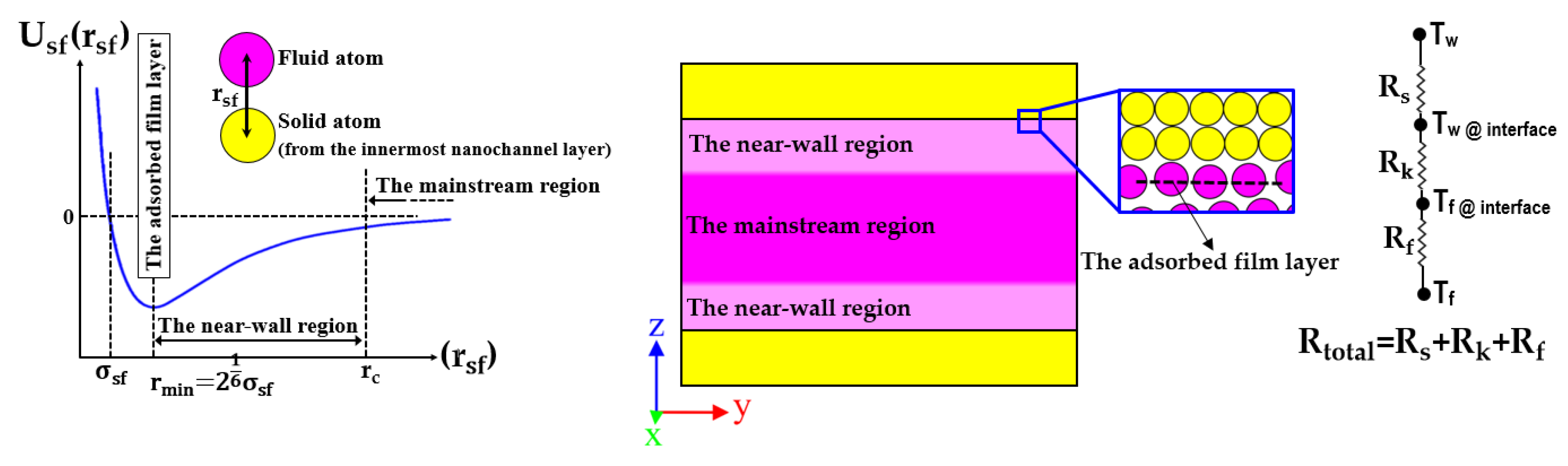
  19. Yao, S.; Wang, J.; Jin, S.; Tan, F.; Chen, S. Atomistic insights into the microscope mechanism of solid–liquid interaction influencing convective heat transfer of nanochannel. J. Mol. Liq. 2023, 371, 121105. [Google Scholar] [CrossRef]
  20. Thekkethala, J.F.; Sathian, S.P. The effect of graphene layers on interfacial thermal resistance in composite nanochannels with flow. Microfluid. Nanofluid. 2015, 18, 637–648. [Google Scholar] [CrossRef]
  21. Markvoort, A.J.; Hilbers, P.A.J. Molecular dynamics study of the influence of wall-gas interactions on heat flow in nanochannels. Phys. Rev. 2005, 71, 066702. [Google Scholar] [CrossRef] [PubMed]
  22. Yao, S.; Wang, J. Effect of rough morphology on the flow and heat transfer in nanochannel. In Proceedings of the International Conference on Applied Energy, Bangkok, Thailand, 1–10 December 2020. [Google Scholar]
  23. Yao, S.; Wang, J.; Liu, X. The influence of wall properties on convective heat transfer in isothermal nanochannel. J. Mol. Liq. 2021, 324, 115100. [Google Scholar] [CrossRef]
  24. Yao, S.; Wang, J.; Liu, X. Role of wall-fluid interaction and rough morphology in heat and momentum exchange in nanochannel. Appl. Energy 2021, 298, 117183. [Google Scholar] [CrossRef]
  25. Yao, S.; Wang, J.; Liu, X. Influence of nanostructure morphology on the heat transfer and flow characteristics in nanochannel. Int. J. Therm. Sci. 2021, 165, 106927. [Google Scholar] [CrossRef]
  26. Yao, S.; Wang, J.; Liu, X. The impacting mechanism of surface properties on flow and heat transfer features in nanochannel. Int. J. Heat Mass Transf. 2021, 176, 121441. [Google Scholar] [CrossRef]
  27. Yao, S.; Wang, J.; Jin, S.; Tan, F.; Chen, S. Effect of surface coupling characteristics on the flow and heat transfer of nanochannel based on the orthogonal test. Int. J. Therm. Sci. 2024, 203, 109161. [Google Scholar] [CrossRef]
  28. Yao, S.; Wang, J.; Liu, X. The Influencing mechanism of surface wettability on convective heat transfer in copper nanochannel. In Proceedings of the International Conference on Applied Energy, Bangkok, Thailand, 29 November–5 December 2021. [Google Scholar]
  29. Song, Z.; Cui, Z.; Cao, Q.; Lio, Y.; Li, J. Molecular dynamics study of convective heat transfer in ordered rough nanochannels. J. Mol. Liq. 2021, 337, 116052. [Google Scholar] [CrossRef]
  30. Song, Z.; Cui, Z.; Lio, Y.; Cao, Q. Heat transfer and flow characteristics in nanochannels with complex surface topological morphology. Appl. Therm. Eng. 2022, 201, 117755. [Google Scholar] [CrossRef]
  31. Song, Z.; Shang, X.; Cui, Z.; Lio, Y.; Cao, Q. Investigation of surface structure-wettability coupling on heat transfer and flow characteristics in nanochannels. Appl. Therm. Eng. 2023, 218, 119362. [Google Scholar] [CrossRef]
  32. Motlagh, M.B.; Kalteh, M. Molecular dynamics simulation of nanofluid convective heat transfer in a nanochannel: Effect of nanoparticles shape, aggregation and wall roughness. J. Mol. Liq. 2020, 318, 114028. [Google Scholar] [CrossRef]
  33. Motlagh, M.B.; Kalteh, M. Simulating the convective heat transfer of nanofluid Poiseuille flow in a nanochannel by molecular dynamics method. Int. Commun. Heat Mass Transf. 2020, 111, 104478. [Google Scholar] [CrossRef]
  34. Motlagh, M.B.; Kalteh, M. Investigating the wall effect on convective heat transfer in a nanochannel by molecular dynamics simulation. Int. J. Therm. Sci. 2020, 156, 106472. [Google Scholar] [CrossRef]
  35. Assadi, S.; Kalteh, M.; Motlagh, M.B. Investigating convective heat transfer coefficient of nanofluid Couette flow in a nanochannel by molecular dynamics simulation. Mol. Simul. 2022, 48, 702–711. [Google Scholar] [CrossRef]
  36. Chatterjee, S.; Paras, H.H.; Chakraborty, M.A. Review of nano and microscale heat transfer: An experimental and molecular dynamics perspective. Processes 2023, 11, 2769. [Google Scholar] [CrossRef]
  37. Ran, Y.; Bertola, V. Achievements and prospects of molecular dynamics simulations in thermofluid sciences. Energies 2024, 17, 888. [Google Scholar] [CrossRef]
  38. Kim, B.H.; Beskok, A.; Cagin, T. Viscous heating in nanoscale shear driven liquid flows. Microfluid. Nanofluid. 2010, 9, 31–40. [Google Scholar] [CrossRef]
  39. Bao, L.; Priezjev, N.V.; Hu, H.; Luo, K. Effects of viscous heating and wall-fluid interaction energy on rate-dependent slip behavior of simple fluids. Phys. Rev. E 2017, 96, 033110. [Google Scholar] [CrossRef]
  40. Dinh, Q.V.; Vo, T.Q.; Kim, B. Viscous heating and temperature profiles of liquid water flows in copper nanochannel. J. Mech. Sci. Technol. 2019, 33, 3257–3263. [Google Scholar] [CrossRef]
  41. AbdulHussein, W.A.; Abed, A.M.; Mohammad, D.B.; Smaisim, G.F.; Baghaei, S. Investigation of boiling process of different fluids in microchannels and nanochannels in the presence of external electric field and external magnetic field using molecular dynamics simulation. Case Stud. Therm. Eng. 2022, 35, 102105. [Google Scholar] [CrossRef]
  42. Wang, M.; Sun, H.; Cheng, L. Flow condensation heat transfer characteristics of nanochannels with nanopillars: A molecular dynamics study. Langmuir 2021, 37, 14744–14752. [Google Scholar] [CrossRef]
  43. Wang, M.; Sun, Q.; Yang, C.; Cheng, L. Molecular dynamics simulation of thermal de-icing on a nanochannel with hot fluids. J. Mol. Liq. 2022, 354, 118859. [Google Scholar] [CrossRef]
  44. Wang, M.; Sun, H.; Cheng, L. Enhanced heat transfer characteristics of nano heat exchanger with periodic fins: A molecular dynamics study. J. Mol. Liq. 2021, 341, 116908. [Google Scholar] [CrossRef]
  45. Sun, H.; Li, F.; Wang, M.; Xin, G.; Wang, X. Molecular dynamics study of convective heat transfer mechanism in a nano heat exchanger. RSC Adv. 2020, 10, 23097. [Google Scholar] [CrossRef]
  46. Rapaport, D.C. The Art of Molecular Dynamics Simulation, 1st ed.; Cambridge University Press: Cambridge, UK, 2004. [Google Scholar]
  47. Pal, S.; Ray, B.C. Molecular Dynamics Simulation of Nanostructured Materials: An Understanding of Mechanical Behavior, 1st ed.; Taylor & Francis Group: Abingdon, UK, 2020. [Google Scholar]
  48. Sadus, R.J. Molecular Simulation of Fluids: Theory, Algorithms, Object-Orientation, 1st ed.; Elsevier Science: Amsterdam, The Netherlands, 2023. [Google Scholar]
  49. Gonzalez, I.; Law, D. Effect of single nanoparticle diameter on a nanochannel fluid flow and heat transfer. In Proceedings of the ASME 2022 Fluids Engineering Division Summer Meeting, Toronto, ON, Canada, 3–5 August 2022. [Google Scholar]
  50. Tang, Y.; Fu, T.; Mao, Y.; Zhang, Y.; Yuan, W. Molecule dynamics simulation of heat transfer between argon flow and parallel copper plates. J. Nanotechnol. Eng. Med. 2014, 5, 034501. [Google Scholar] [CrossRef]
  51. Guillot, B.A. Reappraisal of what we have learnt during three decades of computer simulations on water. J. Mol. Liq. 2002, 101, 219–260. [Google Scholar] [CrossRef]
  52. Kargar, S.; Baniamerian, Z.; Moran, J.L. Molecular dynamics calculations of the enthalpy of vaporization for different water models. J. Mol. Liq. 2024, 393, 123455. [Google Scholar] [CrossRef]
  53. Berendsen, H.J.C.; Grigera, J.R.; Straatsma, T.P. The Missing Term in Effective Pair Potentials. J. Phys. Chem. 1987, 91, 6269–6271. [Google Scholar] [CrossRef]
  54. Jorgensen, W.L.; Chandrasekhar, J.; Madura, J.D.; Impey, R.W.; Klein, M.L. Comparison of simple potential functions for simulating liquid water. J. Chem. Phys. 1983, 79, 926–935. [Google Scholar] [CrossRef]
  55. Abascal, J.L.F.; Vega, C.A. General purpose model for the condensed phases of water: TIP4P/2005. J. Chem. Phys. 2005, 123, 234505. [Google Scholar] [CrossRef]
  56. Cui, W.; Shen, Z.; Yang, J.; Wu, S. Flow and heat transfer behaviors of water-based nanofluids confined in nanochannel by molecular dynamics simulation. Dig. J. Nanomater. Biostructures 2015, 10, 401–413. [Google Scholar]
  57. Asgari, A.; Nguyen, Q.; Karimipour, A.; Bach, Q.; Hekmatifar, M.; Sabetvand, R. Develop molecular dynamics method to simulate the flow and thermal domains of H2O/Cu nanofluid in a nanochannel affected by an external electric field. Int. J. Thermophys. 2020, 41, 126. [Google Scholar] [CrossRef]
  58. Dehkordi, R.B.; Toghraiea, D.; Hashemian, M.; Aghadavoudi, F.; Akbari, M. Molecular dynamics simulation of ferro-nanofluid flow in a microchannel in the presence of external electric field: Effects of Fe3Oe nanoparticles. Int. Commun. Heat Mass Transf. 2020, 116, 104653. [Google Scholar] [CrossRef]
  59. Qin, Y.; Zhao, J.; Liu, Z.; Wang, C.; Zhang, H. Study on effect of different surface roughness on nanofluid flow in nanochannel by using molecular dynamics simulation. J. Mol. Liq. 2022, 346, 117148. [Google Scholar] [CrossRef]
  60. Yu, H.; Tao, Y.; Zhao, Y.; Sha, J. The effect of flow velocity on the convection in nanochannel. In Proceedings of the International Conference on Manipulation, Manufacturing and Measurement on the Nanoscale, Xi’an, China, 2–6 August 2021. [Google Scholar]
  61. Marable, D.C.; Shin, S.; Nobakht, A.Y. Investigation into the microscopic mechanisms influencing convective heat transfer of water flow in graphene nanochannels. Int. J. Heat Mass Transf. 2017, 109, 28–39. [Google Scholar] [CrossRef]
  62. Kusalik, P.G.; Svishchev, I.M. The spatial structure in liquid water. Science 1994, 265, 1219–1221. [Google Scholar] [CrossRef] [PubMed]
  63. Mahoney, M.W.; Jorgensen, W.L. A five-site model for liquid water and the reproduction of the density anomaly by rigid, nonpolarizable potential functions. J. Chem. Phys. 2000, 112, 8910–8922. [Google Scholar] [CrossRef]
  64. González, M.A.; Abascal, J.L.F. The shear viscosity of rigid water models. J. Chem. Phys. 2010, 132, 096101. [Google Scholar] [CrossRef]
  65. Vega, C.; Abascal, J.L.F. Simulating water with rigid non-polarizable models: A general perspective. Phys. Chem. Chem. Phys. 2011, 13, 19663–19688. [Google Scholar] [CrossRef]
  66. Lee, S.H.; Kim, J. Transport properties of bulk water at 243–550 K: A comparative molecular dynamics simulation study using SPC/E, TIP4P, and TIP4P/2005 water models. Mol. Phys. 2018, 117, 1926–1933. [Google Scholar] [CrossRef]
  67. Mao, Y.; Zhang, Y. Thermal conductivity, shear viscosity and specific heat of rigid water models. Chem. Phys. Lett. 2012, 542, 37–41. [Google Scholar] [CrossRef]
  68. Rick, S.W. A reoptimization of the five-site water potential (TIP5P) for use with Ewald sums. J. Chem. Phys. 2004, 120, 6085–6093. [Google Scholar] [CrossRef]
  69. Luo, K.; Li, W.; Ma, J.; Chang, W.; Huang, G.; Li, C. Silicon microchannels flow boiling enhanced via microporous decorated sidewalls. Int. J. Heat Mass Transf. 2022, 191, 122817. [Google Scholar] [CrossRef]
  70. Chakraborty, P.; Ma, T.; Cao, L.; Wang, Y. Significantly enhanced convective heat transfer through surface modification in nanochannels. Int. J. Heat Mass Transf. 2019, 136, 702–708. [Google Scholar] [CrossRef]
  71. Zhou, K.; Liu, B. Molecular Dynamic Simulation: Fundamentals and Applications, 1st ed.; Elsevier Science: Amsterdam, The Netherlands, 2022. [Google Scholar]
  72. Rosa, P.; Karayiannis, T.G.; Collins, M.W. Single-phase heat transfer in microchannels: The importance of scaling effects. Appl. Therm. Eng. 2009, 29, 3447–3468. [Google Scholar] [CrossRef]
  73. Alavi, S. Molecular Simulations: Fundamentals and Practice, 1st ed.; Wiley-VCH: Weinheim, Germany, 2020; pp. 79–81. [Google Scholar]
  74. Ge, S.; Gu, Y.; Chen, M. A molecular dynamics simulation on the convective heat transfer in nanochannels. Mol. Phys. 2014, 113, 703–710. [Google Scholar] [CrossRef]
  75. Frenkel, D.; Smit, B. Understanding Molecular Simulation: From Algorithms to Applications, 1st ed.; Elsevier Science: Amsterdam, The Netherlands, 2001; pp. 34–35. [Google Scholar]
  76. Li, L.; Liu, Z.; Qi, R. Molecular dynamics simulations in hydrogel research and its applications in energy utilization: A review. Energy Rev. 2024, 3, 100072. [Google Scholar] [CrossRef]
  77. Gennes, P.G. Wetting: Statics and dynamics. Rev. Mod. Phys. 1985, 57, 827. [Google Scholar] [CrossRef]
  78. Wang, M.; Sun, H.; Cheng, L. Investigation of convective heat transfer performance in nanochannels with fractal Cantor structures. Int. J. Heat Mass Transf. 2021, 171, 121086. [Google Scholar] [CrossRef]
  79. Tucker, Q.J.; Ivanov, D.S.; Zhigilei, L.V.; Johnson, R.E.; Bringa, E.M. Molecular dynamics simulation of sputtering from a cylindrical track: EAM versus pair potentials. NIM-B 2005, 228, 163–169. [Google Scholar] [CrossRef]
  80. Sekerka, R.F. Thermal Physics: Thermodynamics and Statistical Mechanics for Scientists and Engineers, 1st ed.; Elsevier Science: Amsterdam, The Netherlands, 2015; pp. 273–274. [Google Scholar]
  81. Sun, H.; Liu, Z.; Xin, G.; Xin, Q.; Zhang, J.; Cao, B.Y.; Wang, X. Thermal and flow characterization in nanochannels with tunable surface wettability: A comprehensive molecular dynamics study. Numer. Heat Transf. Part A Appl. 2020, 78, 231–251. [Google Scholar] [CrossRef]
  82. Fallahzadeh, R.; Bozzoli, F.; Cattani, L.; Azam, M.W. Effect of cross nanowall surface on the onset time of explosive boiling: A molecular dynamics study. Energies 2024, 17, 1107. [Google Scholar] [CrossRef]
  83. Daw, M.S.; Foiles, S.M.; Baskes, M.I. The embedded-atom method: A review of theory and applications. Mater. Sci. Rep. 1993, 9, 251–310. [Google Scholar] [CrossRef]
  84. Wang, W.; Zhang, H.; Tian, C.; Meng, X. Numerical experiments on evaporation and explosive boiling of ultra-thin liquid argon film on aluminum nanostructure substrate. Nanoscale Res. Lett. 2015, 10, 158. [Google Scholar] [CrossRef] [PubMed]
  85. Daw, M.S.; Chandross, M. Simple parameterization of embedded atom method potentials for FCC metals. Acta Mater. 2023, 248, 118771. [Google Scholar] [CrossRef]
  86. Heinz, H.; Vaia, R.A.; Farmer, B.L.; Naik, R.R. Accurate simulation of surfaces and interfaces of face-centered cubic metals using 12-6 and 9-6 Lennard-Jones potentials. J. Phys. Chem. C 2008, 112, 17281–17290. [Google Scholar] [CrossRef]
  87. Din, X.D.; Michaelides, E.E. Kinetic theory and molecular dynamics simulations of microscopic flows. Phys. Fluids. 1997, 9, 3915–3925. [Google Scholar] [CrossRef]
  88. Barrat, J.L.; Bocquet, L. Large slip effect at a nonwetting fluid-solid interface. Phys. Rev. Lett. 1999, 82, 4671. [Google Scholar] [CrossRef]
  89. Hagler, A.T.; Lifson, S.; Dauber, P. Consistent force field studies of intermolecular forces in hydrogen-bonded crystals. 2. a benchmark for the objective comparison of alternative force fields. J. Am. Chem. Soc. 1979, 101, 5122–5130. [Google Scholar] [CrossRef]
  90. Hagler, A.T.; Huler, E.; Lifson, S. Energy functions for peptides and proteins. I. Derivation of a consistent force field including the hydrogen bond from amide crystals. J. Am. Chem. Soc. 1974, 96, 5319–5327. [Google Scholar] [CrossRef]
  91. Waldman, M.; Hagler, A.T. New combining rules for rare gas van der Waals parameters. J. Comput. Chem. 1993, 14, 1077–1084. [Google Scholar] [CrossRef]
  92. Delhommelle, J.; Millie, P. Inadequacy of the Lorentz-Berthelot combining rules for accurate predictions of equilibrium properties by molecular simulation. Mol. Phys. 2001, 99, 619–625. [Google Scholar] [CrossRef]
  93. Weeks, J.D.; Chandler, D.; Andersen, H.C. Role of repulsive forces in determining the equilibrium structure of simple liquids. J. Chem. Phys. 1971, 54, 5237–5247. [Google Scholar] [CrossRef]
  94. Jiang, H.; Patel, A.J. Recent advances in estimating contact angles using molecular simulations and enhanced sampling methods. Curr. Opin. Chem. Eng. 2019, 23, 130–137. [Google Scholar] [CrossRef]
  95. Debye, P.; Erich, H. The theory of electrolytes. I. Freezing point depression and related phenomena. Phys. Z. 1923, 24, 185–206. [Google Scholar]
  96. Nichita, D.V.; Petitfrere, M. Phase equilibrium calculations with quasi-Newton methods. Fluid Phase Equilib. 2015, 406, 194–208. [Google Scholar] [CrossRef]
  97. Hestenes, M.R.; Stiefel, E. Methods of conjugate gradients for solving linear systems. J. Res. Natl. Bur. Stand. 1952, 49, 2379. [Google Scholar] [CrossRef]
  98. Hoover, W.G. Canonical dynamics: Equilibrium phase-space distributions. Phys. Rev. A 1985, 31, 1695. [Google Scholar] [CrossRef]
  99. Chen, W.-H.; Wu, C.-H.; Cheng, H.-C. Modified Nosé-Hoover thermostat for solid state for constant temperature molecular dynamics simulation. J. Comput. Phys. 2011, 230, 6354–6366. [Google Scholar] [CrossRef]
  100. Rowlinson, J.S. The maxwell–Boltzmann distribution. Mol. Phys. 2005, 103, 2821–2828. [Google Scholar] [CrossRef]
  101. Hu, C.; Bai, M.; Lv, J.; Li, X. An investigation on the flow and heat transfer characteristics of nanofluid by nonequilibrium molecular dynamics simulations. Numer. Heat Transf. Part B 2016, 70, 152–163. [Google Scholar] [CrossRef]
  102. Ashurst, W.T.; Hoover, W.G. Dense-fluid shear viscosity via nonequilibrium molecular dynamics. Phys. Rev. A 1975, 11, 658. [Google Scholar] [CrossRef]
  103. Khare, R.; de Pablo, J.; Yethiraj, A. Molecular simulation and continuum mechanics study of simple fluids in non-isothermal planar couette flows. J. Chem. Phys. 1997, 107, 2589–2596. [Google Scholar] [CrossRef]
  104. Zheng, B.; Huang, Z.; Zheng, Z.; Chen, Y.; Yan, J.; Cen, K.; Yang, H.; Ostrikov, K. Accelerated ion transport and charging dynamics in more ionophobic sub-nanometer channels. Energy Storage Mater. 2023, 59, 102797. [Google Scholar] [CrossRef]
  105. Fallahzadeh, R.; Bozzoli, F.; Cattani, L. Effect of closed-loop nanochannels on the onset of explosive boiling: A molecular dynamics simulation study. J. Phys. Conf. Ser. 2024, 2685, 012013. [Google Scholar] [CrossRef]
  106. Hu, H.; Lu, Y.; Guo, L.; Chen, X.; Wang, Q.; Wang, J.; Li, Q. Effects of system pressure on nucleate boiling: Insights from molecular dynamics. J. Mol. Liq. 2024, 402, 124745. [Google Scholar] [CrossRef]
  107. Barisik, M.; Beskok, A. Boundary treatment effects on molecular dynamics simulations of interface thermal resistance. J. Comput. Phys. 2012, 231, 7881–7892. [Google Scholar] [CrossRef]
  108. Qin, S.; Chen, Z.; Wang, Q.; Li, W.; Xing, H. Effect of surface structure on fluid flow and heat transfer in cold and hot wall nanochannels. Int. J. Heat Mass Transf. 2024, 151, 107257. [Google Scholar] [CrossRef]
  109. Schneider, T.; Stoll, E. Molecular-dynamics study of a three-dimensional one-component model for distortive phase transitions. Phys. Rev. B 1978, 17, 1302. [Google Scholar] [CrossRef]
  110. Berendsen, H.J.; Postma, J.V.; Van Gunsteren, W.F.; DiNola, A.R.H.J.; Haak, J.R. Molecular dynamics with coupling to an external bath. J. Chem. Phys. 1984, 81, 3684–3690. [Google Scholar] [CrossRef]
  111. Thomas, T.M.; Vinod, N. Convective heat transfer between liquid argon flows and heated carbon nanotube arrays using molecular dynamics. J. Appl. Fluid Mech. 2019, 12, 971–980. [Google Scholar] [CrossRef]
  112. Gu, Y.W.; Ge, S.; Chen, M. A molecular dynamics simulation of nanoscale convective heat transfer with the effect of axial heat conduction. Mol. Phys. 2016, 114, 1922–1930. [Google Scholar] [CrossRef]
  113. Yu, F.; Wang, T.; Zhang, C. Effect of axial conduction on heat transfer in a rectangular microchannel with local heat flux. J. Therm. Sci. Technol. 2018, 13, JTST0013. [Google Scholar] [CrossRef]
  114. Cole, K.D.; Çetin, B. The effect of axial conduction on heat transfer in a liquid microchannel flow. Int. J. Heat Mass Transf. 2011, 54, 2542–2549. [Google Scholar] [CrossRef]
  115. Chen, C.; Li, Y. Studying the influence of surface roughness with different shapes and quantities on convective heat transfer of fluid within nanochannels using molecular dynamics simulations. J. Mol. Model. 2024, 30, 42. [Google Scholar] [CrossRef]
  116. Stojanovic, N.; Maithripala, D.H.S.; Berg, J.M.; Holtz, M.J.P.R. Thermal conductivity in metallic nanostructures at high temperature: Electrons, phonons, and the Wiedemann-Franz law. Phys. Rev. B 2010, 82, 075418. [Google Scholar] [CrossRef]
  117. Heino, P.; Ristolainen, E. Thermal conduction at the nanoscale in some metals by MD. Microelectron. J. 2003, 34, 773–777. [Google Scholar] [CrossRef]
  118. Stamper, C.; Cortie, D.; Yue, Z.; Wang, X.; Yu, D. Experimental confirmation of the universal law for the vibrational density of states of liquids. J. Phys. Chem. Lett. 2022, 13, 3105–3111. [Google Scholar] [CrossRef] [PubMed]
  119. Peethan, A.; Unnikrishnan, V.K.; Chidangil, S.; George, S.D. Laser-Assisted tailoring of surface wettability-fundamentals and applications: A critical review. Prog. Adhes. Adhesives. 2020, 5, 331–365. [Google Scholar] [CrossRef]
  120. Zhang, C.B.; Xu, Z.L.; Chen, Y.P. Molecular dynamics simulation on fluid flow and heat transfer in rough nanochannels. Acta Phys. Sin. 2014, 63, 214706. [Google Scholar] [CrossRef]
  121. Zhang, T.; Cui, T. Enhanced wetting properties of silicon mesh microchannels coated with SiO2/SnO2 nanoparticles through layer-by-layer self-assembly. Sens. Actuators B Chem. 2011, 157, 697–702. [Google Scholar] [CrossRef]
  122. Wu, H.Y.; Cheng, P. An experimental study of convective heat transfer in silicon microchannels with different surface conditions. Int. J. Heat Mass Transf. 2003, 46, 2547–2556. [Google Scholar] [CrossRef]
  123. Toghraie, D.; Mokhtari, M.; Afrand, M. Molecular dynamic simulation of Copper and Platinum nanoparticles Poiseuille flow in a nanochannels. Physica. E 2016, 84, 152–161. [Google Scholar] [CrossRef]
  124. Fu, T.; Wang, Q. Effect of nanostructure on heat transfer between fluid and copper plate: A molecular dynamics simulation study. Mol. Simul. 2018, 44, 697–702. [Google Scholar] [CrossRef]
  125. Liu, H.; Deng, W.; Ding, P.; Zhao, J. Investigation of the effects of surface wettability and surface roughness on nanoscale boiling process using molecular dynamics simulation. Nucl. Eng. Des. 2021, 382, 111400. [Google Scholar] [CrossRef]
  126. Liu, H.; Qin, X.; Ahmad, S.; Tong, Q.; Zhao, J. Molecular dynamics study about the effects of random surface roughness on nanoscale boiling process. Int. J. Heat Mass Transf. 2019, 145, 118799. [Google Scholar] [CrossRef]
  127. Fallahzadeh, R.; Bozzoli, F.; Cattani, L.; Pagliarini, L.; Naeimabadi, N.; Azam, M.W. A molecular dynamics perspective on the impacts of random rough surface, film thickness, and substrate temperature on the adsorbed film’s liquid-vapor phase transition regime. Sci 2024, 6, 33. [Google Scholar] [CrossRef]
  128. Piekiel, N.W.; Morris, C.J.; Currano, L.J.; Lunking, D.M.; Isaacson, B.; Churaman, W.A. Enhancement of on-chip combustion via nanoporous silicon microchannels. Combust. Flame 2014, 161, 1417–1424. [Google Scholar] [CrossRef]
  129. Morshed, A.M.; Rezwan, A.A.; Khan, J.A. Two-phase convective flow in microchannel with nanoporous coating. Procedia Eng. 2014, 90, 588–598. [Google Scholar] [CrossRef]
  130. Ahmad, S.; Deng, W.; Liu, H.; Khan, S.A.; Chen, J.; Zhao, J. Molecular dynamics simulations of nanoscale boiling on mesh-covered surfaces. Appl. Therm. Eng. 2021, 195, 117183. [Google Scholar] [CrossRef]
  131. Ahmad, S.; Khan, S.A.; Ali, H.M.; Huang, X.; Zhao, J. Molecular dynamics study of nanoscale boiling on double layered porous meshed surfaces with gradient porosity. Appl. Nanosci. 2022, 12, 2997–3006. [Google Scholar] [CrossRef]
  132. Guan, S.Y.; Zhang, Z.H.; Wu, R.; Gu, X.K.; Zhao, C.Y. Boiling on nano-porous structures: Theoretical analysis and molecular dynamics simulations. Int. J. Heat Mass Transf. 2022, 191, 122848. [Google Scholar] [CrossRef]
  133. Islam, M.A.; Rony, M.D.; Hasan, M.N. Thin film liquid-vapor phase change phenomena over nano-porous substrates: A molecular dynamics perspective. Heliyon 2023, 9, e15714. [Google Scholar] [CrossRef]
  134. Gürdal, M.; Arslan, K.; Gedik, E.; Minea, A.A. Effects of using nanofluid, applying a magnetic field, and placing turbulators in channels on the convective heat transfer: A comprehensive review. Renew. Sustain. Energy Rev. 2022, 162, 112453. [Google Scholar] [CrossRef]
  135. Wen, D.; Ding, Y. Experimental investigation into convective heat transfer of nanofluids at the entrance region under laminar flow conditions. Int. J. Heat Mass Transf. 2004, 47, 5181–5188. [Google Scholar] [CrossRef]
  136. Yang, Y.; Zhang, Z.G.; Grulke, E.A.; Anderson, W.B.; Wu, G. Heat transfer properties of nanoparticle-in-fluid dispersions (nanofluids) in laminar flow. Int. J. Heat Mass Transf. 2005, 48, 1107–1116. [Google Scholar] [CrossRef]
  137. Sun, H.; Wang, M. Atomistic insights into heat transfer and flow behaviors of nanofluids in nanochannels. J. Mol. Liq. 2022, 345, 117872. [Google Scholar] [CrossRef]
  138. Hashemi, S.M.H.; Fazeli, S.A.; Zirakzadeh, H.; Ashjaee, M. Study of heat transfer enhancement in a nanofluid-cooled miniature heat sink. Int. Commun. Heat Mass Transf. 2012, 39, 877–884. [Google Scholar] [CrossRef]
  139. Sakanova, A.; Keian, C.C.; Zhao, J. Performance improvements of microchannel heat sink using wavy channel and nanofluids. Int. J. Heat Mass Transf. 2015, 89, 59–74. [Google Scholar] [CrossRef]
  140. Rahimi-Gorji, M.; Pourmehran, O.; Hatami, M.; Ganji, D.D. Statistical optimization of microchannel heat sink (MCHS) geometry cooled by different nanofluids using RSM analysis. Eur. Phys. J. Plus. 2015, 130, 22. [Google Scholar] [CrossRef]
  141. Shahrestani, M.I.; Maleki, A.; Shadloo, M.S.; Tlili, I. Numerical investigation of forced convective heat transfer and performance evaluation criterion of Al2O3/water nanofluid flow inside an axisymmetric microchannel. Symmetry 2020, 12, 120. [Google Scholar] [CrossRef]
  142. Lin, X.; Mo, S.; Jia, L.; Yang, Z.; Chen, Y.; Cheng, Z. Experimental study and Taguchi analysis on LED cooling by thermoelectric cooler integrated with microchannel heat sink. Appl. Energy 2019, 242, 232–238. [Google Scholar] [CrossRef]
Figure 1. Schematic representations of (a) slip velocity and slip length and (b) temperature jump length (considering a hot Poiseuille flow through a cold nanochannel).
Energies 17 04352 g001
Figure 2. A simplified flowchart of the sequence of the MD simulation steps for studying FCHT-NC.
Energies 17 04352 g002
Figure 3. Schematic representations and key parameters of various water models used in the MD simulation of FCHT-NC: (a) SPC/E and (b) TIP4P and TIP4P/2005 [17,28,56,57,58,59,60,61]. Red, white, and green spheres indicate O atoms, H atoms, and the mass-less but charged site (the dummy atom). The parameter data for SPC/E, TIP4P, and TIP4P/2005 are taken from Refs. [62], [63] and [55], respectively. * Å (angstrom) = 10−10 m.
Energies 17 04352 g003
Figure 4. A schematic representation of a typical initial simulation box. The green, red, and blue slender arrows represent the x, y, and z axes, respectively.
Energies 17 04352 g004
Figure 5. Schematic representations of the initial positions of the fluid particles in the initial simulation box: (a) ordered structure and (b) randomly distributed. The yellow and purple circles indicate the nanochannel wall atoms and fluid particles, respectively.
Energies 17 04352 g005
Figure 6. (a) shows schematic representation of duplicating the initial simulation box in the x-direction. (b) shows when an atom exits the simulation box on one side, an equivalent image atom from an adjacent imaginary box enters the sim-ulation box from the opposite side. Schematic representations of the periodic boundary condition concept in the x-direction. The yellow, purple, and olive circles indicate the nanochannel wall, fluid domain, and imaginary atoms, respectively.
Energies 17 04352 g006
Figure 7. Schematic representations of (a) gravity-driven, (b) pressure-driven, (c) atomistic wall, and (d) fluid-like wall models to create flow within the nanochannels. The yellow and purple circles indicate the nanochannel wall and fluid atoms, respectively. The green, red, and blue slender arrows represent the x, y, and z axes, respectively. The wide green arrow represents the external force.
Energies 17 04352 g007
Figure 8. Schematic representations of (a) all-wall thermostat and (b) partial-wall thermostat models. The green, red, and blue slender arrows represent the x, y, and z axes, respectively. The brown, green, yellow, and purple circles indicate the fixed, temperature control, thermal conductive, and fluid atoms, respectively.
Energies 17 04352 g008
Figure 9. Schematic representations of temperature control areas (with an NVT ensemble) in (a) Couette flow and (b) Poiseuille flow models. The yellow and purple areas indicate the nanochannel wall and fluid domains, respectively. The purple crosshatch area shows the fluid domain without temperature control (and with an NVE ensemble). The green, red, and blue slender arrows represent the x, y, and z axes, respectively.
Energies 17 04352 g009
Figure 10. Schematic representations of (a) Markvoort and (b) Ge thermal pump methods and (c) axial heat conduction at the outlet. The black arrows represent the fluid flow direction.
Energies 17 04352 g010
Figure 11. A schematic representation of divided fluid domain along the y- and z-directions.
Energies 17 04352 g011
Figure 12. Simplified schematic representations of the two-dimensional temperature distributions in the y–z plane and the average temperature variation along the flow direction (the red curved dashed line).
Energies 17 04352 g012
Figure 13. Schematic representation of three defined fluid regions and the thermal resistance network. The yellow and purple areas indicate the nanochannel walls and fluid domain, respectively.
Energies 17 04352 g013
Figure 14. Overlap of the VDOS of the coating material with both the solid nanochannel wall atoms and the near-wall fluid atoms (reprinted from Ref. [70], Copyright 2024, with permission from Elsevier, Amsterdam, the Netherlands).
Energies 17 04352 g014
Figure 15. Schematic representations of different surface roughness morphologies. The green, red, and blue slender arrows represent the x, y, and z axes, respectively.
Energies 17 04352 g015
Figure 16. Variation of the local Nu number in the presence of simple periodic sinusoidal nanostructures (reprinted from Ref. [29], Copyright 2024, with permission from Elsevier, Amsterdam, the Netherlands).
Energies 17 04352 g016
Figure 17. A schematic representation of the deposited, suspended nanoparticles and the spinning and Brownian motions. The yellow and purple areas indicate the nanochannel wall and fluid domains, respectively.
Energies 17 04352 g017
Figure 18. Variation of Nu number as a function of the channel height (reprinted from Ref. [61], Copyright 2024, with permission from Elsevier, Amsterdam, the Netherlands).
Energies 17 04352 g018
Figure 19. Variation of Nu number as a function of the nanochannel wall temperature (reprinted from Ref. [61], Copyright 2024, with permission from Elsevier, Amsterdam, the Netherlands).
Energies 17 04352 g019
Table 1. The length and energy parameters in the LJ 12–6 potential for common solid wall materials.
Atom Pair σ ε Reference
Cu-Cu2.340 Å0.4096 eV *[31]
Pt-Pt2.475 Å0.521 eV *[78]
* eV = 96.485 kJ/mol.
Table 2. The length and energy parameters in the LJ 12–6 potential for common fluid materials.
Atom PairWater Model σ ε Reference
Ar-Ar-3.405 Å0.01043 eV[27]
O-OSPC/E3.166 Å0.650 kJ/mol[62]
TIP4P3.15365 Å0.6480 kJ/mol[63]
TIP4P/20053.1589 Å0.7749 kJ/mol[55]
Table 3. Classification of surface wettability based on the contact angle.
Nature of the SurfaceContact Angle (Degree)
Super-hydrophilic 0     θ     30
Hydrophilic 30   <   θ   <   90
Neutral θ = 90
Hydrophobic 90   <   θ   <   150
Super-hydrophobic 150     θ     180
Table 4. A summary of MD simulation studies regarding surface wettability.
Author(s)/YearFluid/Wall MaterialsNature of the Studied Surfaces
Markvoort et al. [21]/2005CLJ/CLJSuper-hydrophilic, Hydrophobic
Ge et al. [74]/2014Ar/CLJSuper-hydrophilic, Neutral
Cheng-Bin et al. [120]/2014CLJ/CLJSuper-hydrophilic, Neutral, Hydrophobic
Gu et al. [112]/2016Ar/PtSuper-hydrophilic, Hydrophilic, Neutral
Marable et al. [71]/2017water/grapheneSuper-hydrophilic, Hydrophilic, Neutral, Hydrophobic
Yao and Wang [22]/2020Ar/PtSuper-hydrophilic, Hydrophobic
Sun et al. [81]/2020Ar/CuSuper-hydrophilic, Hydrophilic, Hydrophobic
Yao et al. [23]/2021Ar/CLJSuper-hydrophilic, Neutral
Yao et al. [24]/2021Ar/PtSuper-hydrophilic, Hydrophobic
Wang et al. [78]/2021Ar/PtSuper-hydrophilic, Hydrophilic
Yao et al. [25]/2021Ar/PtSuper-hydrophilic, Hydrophobic
Yao et al. [26]/2021Ar/PtSuper-hydrophilic, Hydrophobic
Yao et al. [28]/2021water/CuHydrophilic, Hydrophobic
Song et al. [31]/2023Ar/CuSuper-hydrophilic, Hydrophilic, Hydrophobic
Yao et al. [19]/2023Ar/PtSuper-hydrophilic, Hydrophilic, Neutral, Hydrophobic
Yao et al. [27]/2024Ar/PtSuper-hydrophilic, Hydrophilic, Neutral, Hydrophobic
Table 5. A summary of MD simulation studies regarding surface coating.
Author(s)/YearFluid/Wall MaterialsCoating Material
Thekkethala and Sathian [20]/2015Ar/Cugraphene
Chakraborty et al. [70]/2019Ar/CLJCLJ
Yao et al. [23]/2021Ar/CLJCLJ
Yao et al. [27]/2024Ar/CLJCLJ
Table 6. A summary of MD simulation studies regarding surface roughness.
Author(s)/YearWall MaterialSurface Roughness Morphology
Cheng-Bin et al. [120]/2014CLJUniform rectangle nanostructure
Toghraie et al. [123]/2016PtUniform rectangle nanostructure
Fu and Wang [124]/2018CuUniform rectangle nanostructure
Chakraborty et al. [70]/2019CLJUniform rectangle nanostructure
Non-uniform rectangle nanostructure
Motlagh and Kalteh [32]/2020CuUniform rectangle nanostructure
Motlagh and Kalteh [34]/2020CuUniform rectangle nanostructure
Yao and Wang [22]/2020PtUniform rectangle nanostructure
Asgari et al. [57]/2020CuUniform hemispherical nanostructure
Song et al. [29]/2021CuSimple periodic sinusoidal nanostructure
Yao et al. [24]/2021PtUniform rectangle nanostructure
Yao et al. [25]/2021PtUniform rectangle nanostructure
Wang et al. [78]/2021PtNon-uniform rectangle nanostructure
Yao et al. [26]/2021PtUniform rectangle nanostructure
Song et al. [29]/2022CuSimple periodic sinusoidal nanostructure
Subdivided periodic sinusoidal nanostructure
Song et al. [31]/2023CuSimple periodic sinusoidal nanostructure
Subdivided periodic sinusoidal nanostructure
Qin et al. [108]/2024PtUniform rectangle nanostructure
Uniform triangular nanostructure
Chen and Li [115]/2024CuUniform rectangle nanostructure
Uniform triangular nanostructure
Uniform hemispherical nanostructure
Yao et al. [27]/2024PtUniform rectangle nanostructure
Table 7. A summary of MD simulation studies regarding nanofluids.
Energies 17 04352 i001
Cylindrical nanoparticleSpherical nanoparticle
Author(s)/YearBase Fluid/Wall
Materials
Nanoparticles
MaterialShapeDimensions (Å)Number of
Nanoparticles
Cui et al. [56]/2015water/CuCusphereD = 401
Hu et al. [102]/2016Ar/CuCusphereD = 20, 24 and 301 and 3
Toghraie et al. [123]/2016Ar/PtCu and PtsphereD 602, 3 and 4
Motlagh and Kalteh [33]/2020Ar/CuCusphereD = 8, 10 and 12.61, 2, 3 and 4
Motlagh and Kalteh [32]/2020Ar/CuCucylinderL = 9.5 and D = 64
Dehkordi et al. [58]/2020/CuFe3O4sphereD = 250, 500 and 7001, 2 and 3
Assadi et al. [35]/2020Ar/CuCusphereD = 12.64, 15 and 163, 4 and 5
Gonzalez and Law [49]/2022Ar/CuCusphereD = 8, 10, 15, 17.5 and 201
Sun and Wang [137]/2022Ar/CuCusphereD 740 and 80
Disclaimer/Publisher’s Note: The statements, opinions and data contained in all publications are solely those of the individual author(s) and contributor(s) and not of MDPI and/or the editor(s). MDPI and/or the editor(s) disclaim responsibility for any injury to people or property resulting from any ideas, methods, instructions or products referred to in the content.

