Article

Optimal Design of an Interior Permanent Magnet Synchronous Motor for Electric Vehicle Applications Using a Machine Learning-Based Surrogate Model

by
Song Guo
,
Xiangdong Su
and
Hang Zhao
*
Robotics and Autonomous Systems Thrust, The Hong Kong University of Science and Technology (Guangzhou), Guangzhou 511453, China
*
Author to whom correspondence should be addressed.
Energies 2024, 17(16), 3864; https://doi.org/10.3390/en17163864
Submission received: 29 June 2024 / Revised: 29 July 2024 / Accepted: 1 August 2024 / Published: 6 August 2024
(This article belongs to the Section F: Electrical Engineering)

Abstract

:
This paper presents an innovative design for an interior permanent magnet synchronous motor (IPMSM), targeting enhanced performance for electric vehicle (EV) applications. The proposed motor features a double V-shaped rotor structure with irregular ferrite magnets embedded in the slots between the permanent magnets. This design significantly enhances torque performance. Furthermore, a machine learning-based surrogate model is developed by integrating fine and coarse mesh data. Optimized using the Non-dominated Sorting Genetic Algorithm II (NSGA-II), this surrogate model effectively reduces computational time compared to traditional finite element analysis (FEA).

1. Introduction

Global warming and the depletion of fossil fuels are issues that humanity must address. Electric vehicles (EVs) rely on a modern electric system consisting of motors, power converters, batteries, and controllers instead of internal combustion engines (ICEs). EVs offer significant environmental benefits, including zero emissions, low noise, light weight, improved performance, and efficiency [1,2]. As an essential component of EVs, motors play a crucial role in achieving these benefits. Meanwhile, the application of electric vehicles also faces several challenges. The primary issues currently include the short driving range of electric vehicles, the long charging times required, the underdeveloped deployment of charging stations, and the lack of standardization in charging connectors. Additionally, problems related to battery capacity, safety, and cost need to be addressed. Moreover, the optimization of battery management systems is crucial [3]. In [4], a method of utilizing supercapacitors in the starting system of diesel locomotives was proposed, which effectively enhances the system’s service life. Research on motor design optimization has focused on various types of motors. N. Zhao et al. [5] designed a 120 kW induction motor and proposed a design method with parameter optimization. B. Dianati et al. [6] optimized an axial flux induction motor (AFIM), which is an attractive alternative to the conventional radial flux induction motors (IMs) for EV applications. Synchronous reluctance motors (SynRMs) have a cost advantage over interior permanent magnet motors. Y. Guan et al. [7] designed SynRM, ferrite-assisted SynRM, and NdFeB-assisted SynRM with the same stator outer diameter and stack length and compared the results. In [8], an optimization method for high-speed SynRMs utilizing topology optimization was proposed, which ensures the mechanical strength of the motor at high rotational speeds. M. D. Nardo et al. [9] designed and optimized a 5 kW, 80,000 rpm high-speed SynRM. Permanent magnet synchronous motors (PMSMs) are widely used in EVs due to their high torque density and efficiency [10,11,12,13,14,15]. PMSMs are mainly divided into surface-mounted permanent magnet synchronous motors (SPMSMs) and interior permanent magnet synchronous motors (IPMSMs). SPMSMs have a simple structure and are easy to manufacture. In [15], a simple six-phase surface-mounted permanent magnet field modulation motor was designed. But when the motor operates at high speeds, the surface-mounted permanent magnets on the rotor may be subjected to significant centrifugal forces, potentially leading to mechanical strength issues. IPMSMs enhance mechanical strength at high speeds by embedding the magnets within the rotor [14].
Designing and optimizing motors for EV applications involves a multifaceted set of considerations due to the challenging driving conditions they must navigate. Unlike traditional motors, the development of EV motors must account for a range of factors. These include delivering consistent torque, minimizing torque fluctuations and cogging torque, reducing core losses, maintaining high efficiency across various operational states, ensuring the rotor’s structural integrity, and managing costs [16,17].
Motor design optimization is a general means to improve motor performance and enhance robustness. For PMSMs, due to the pursuit of excellent performance and meeting various demanding requirements, it is necessary to design complex topologies and a large number of geometric variables to build motor models [18].
For the optimization of PMSMs, one strategy is based on the calculation method of the Magnetic Equivalent Circuits (MEC) model, but this method has a problem in calculating nonlinear parameters [19]. FEA, combined with optimization algorithms, can avoid this problem.
The design optimization problem of PMSMs becomes dimensionally expensive as more variables and undetermined boundaries are involved. Optimization based on traditional finite elements requires a lot of calculations, and for some more complex designs that are 3D or used for fine design, the computational burden of FEA is immeasurable or even almost impossible to complete. Therefore, scholars have proposed motor optimization methods based on the surrogate model [20].
Response surface methodology (RSM) is used to build models. Monte Carlo methods help improve model accuracy [21]. However, for some sensitive targets, the model response may be significantly biased by simply aggregating multiple response surfaces. Negative effects are caused by traditional response surface generation or model-building algorithms, such as spline interpolation, kriging interpolation, linear regression, quadratic regression, etc. The method based on machine learning can theoretically fit any function, so the machine learning method is applied to the establishment of agent models and motor optimization [22].
There have been some studies on EV motors based on machine learning. In [23], a six-phase PMSM was designed and optimized by using machine learning technology, and support vector regression (SVR) was used there. M. R. Raia et al. [24] studied the dimensionality reduction equivalence of motor models using an artificial neural network (ANN). In [25], a method for generating motor geometry based on machine learning and image processing was proposed. This method combines image processing and deep neural networks to learn motor geometry images as input.
This paper proposes a method to improve motor performance by adding ferrite permanent magnets in the gaps between the slots and the existing permanent magnets and proposes a surrogate model based on machine learning that applies lesser amounts of fine mesh model data and substantial amounts of coarse mesh model mesh data to balance accuracy and computational burden. Section 2 introduces the motor mechanism, and Section 3 is about the specific model algorithm and results, followed by the discussion and conclusion.

2. Model of IPMSM with the Addition of Ferrite

2.1. Motor Structure

The overall structure of the eight-pole, forty-eight-slot (8P48S) interior PMSM is shown in Figure 1. The motor model consists of the core, magnets, rotor core, stator core, and winding. The magnet placement in the rotor adopts a double V-shaped structure. The stator and rotor cores are made of steel, specifically 50CS1000 (China Steel Corporation, Taiwan, China), while the winding is copper. There are two types of magnetic pole materials: neodymium iron boron (NdFeB) and ferrite.

2.2. Structure Selection and Analysis

Due to technological and material limitations, NdFeB magnets are typically made into regular shapes like squares or tiles. The irregular slots for embedding these magnets are designed to improve the magnetic circuit and overall motor performance. This design, however, leaves gaps that can waste potential performance.
Ferrite materials, on the other hand, can be processed into irregular shapes and embedded into these gaps, making full use of the space and enhancing motor performance [26]. The study compares motor performance with three different magnetization methods: no ferrite filling (air), Halbach arrangement, and parallel magnetization, which are presented in Figure 2. For structure a (air), which is the motor structure without adding ferrite, and for structure b (Halbach), this structure is selected due to its magnetic focusing effect. This method has already been used in research on brushless DC (BLDC) motors, and studies have shown that this Halbach method can improve motor performance [27,28]. For structure c (parallel), the same magnetization direction as NdFeB is used. The idea is to utilize previously unused areas to enhance the permanent magnet flux linkage of the motor.
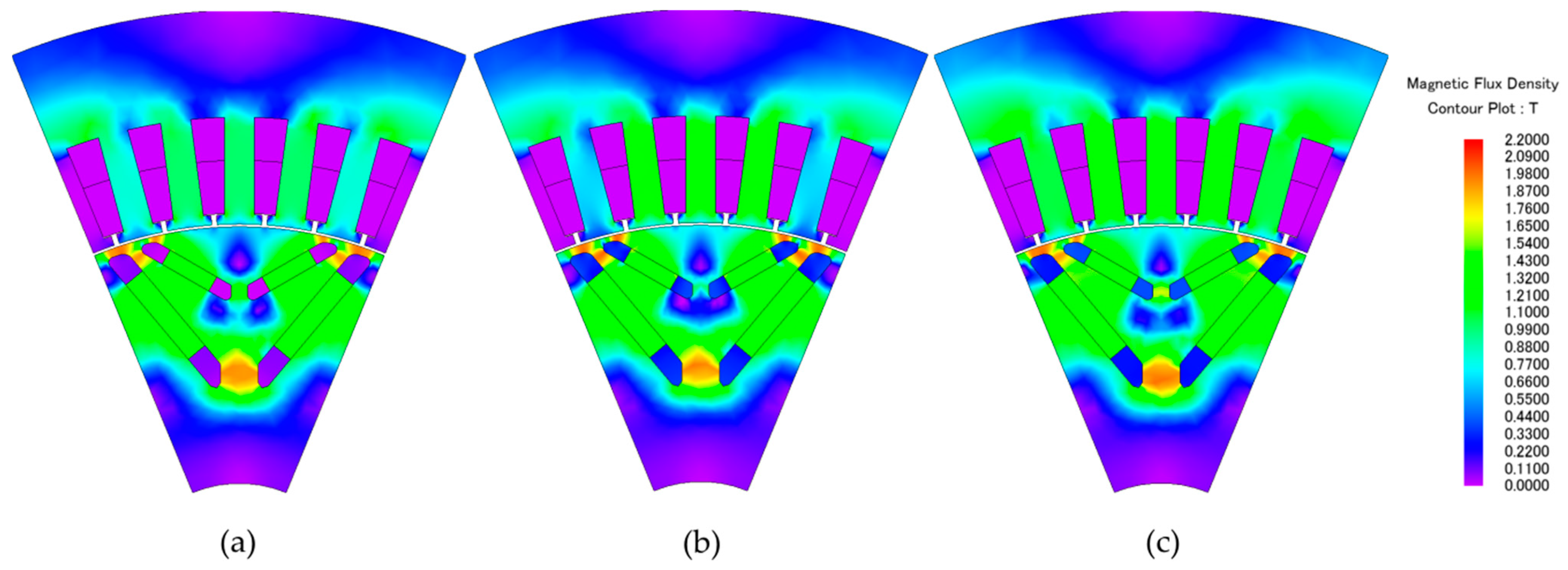
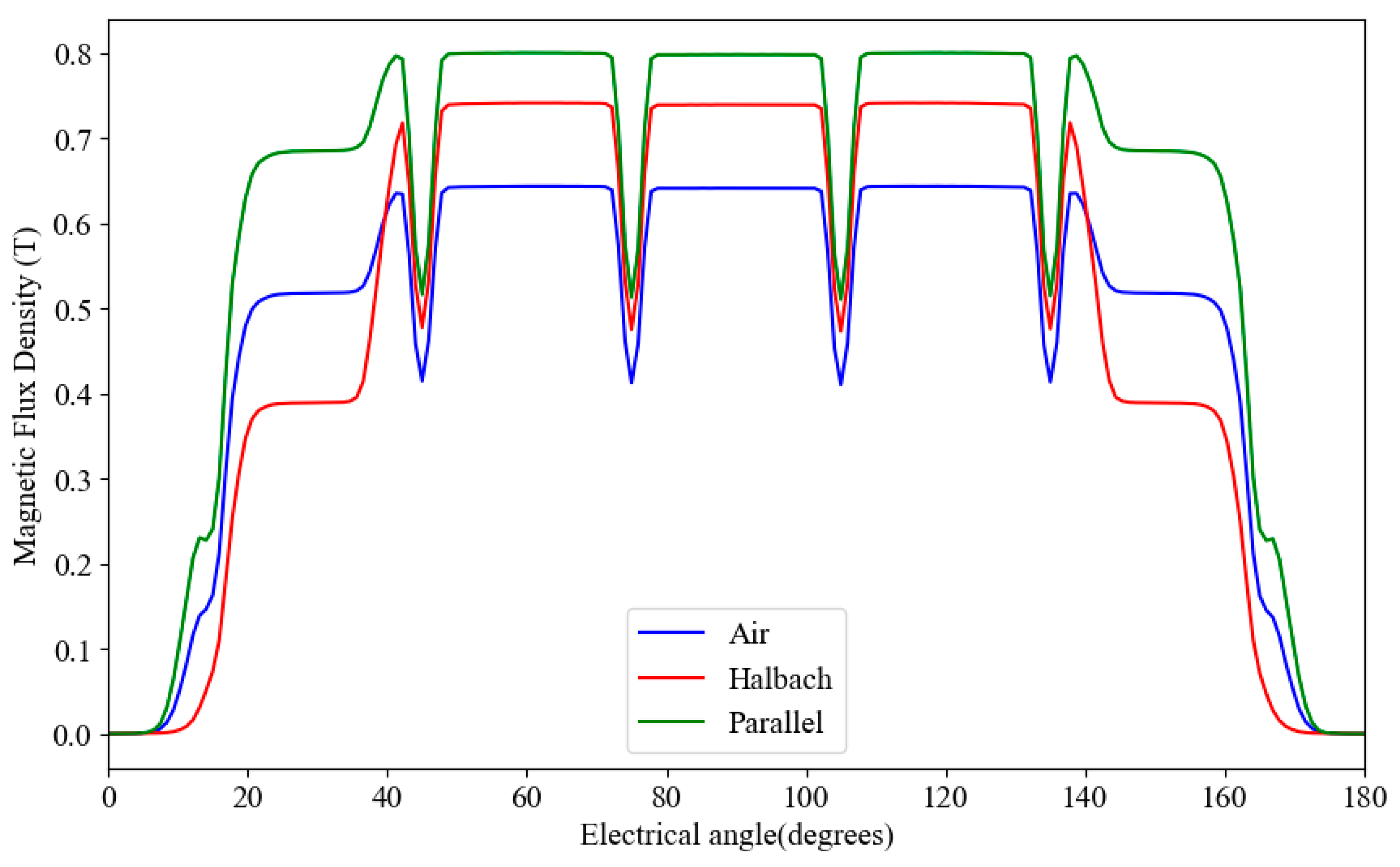
The magnetic flux density diagrams of the three structures are shown in Figure 3. Compared to the structure without ferrite, the addition of ferrite enhances and concentrates the magnetic field. Figure 4 shows the air gap magnetic flux density diagrams for the three structures, where the structures with ferrite have significantly increased air gap magnetic flux density, with the parallel magnetization method resulting in the highest air gap magnetic flux density.
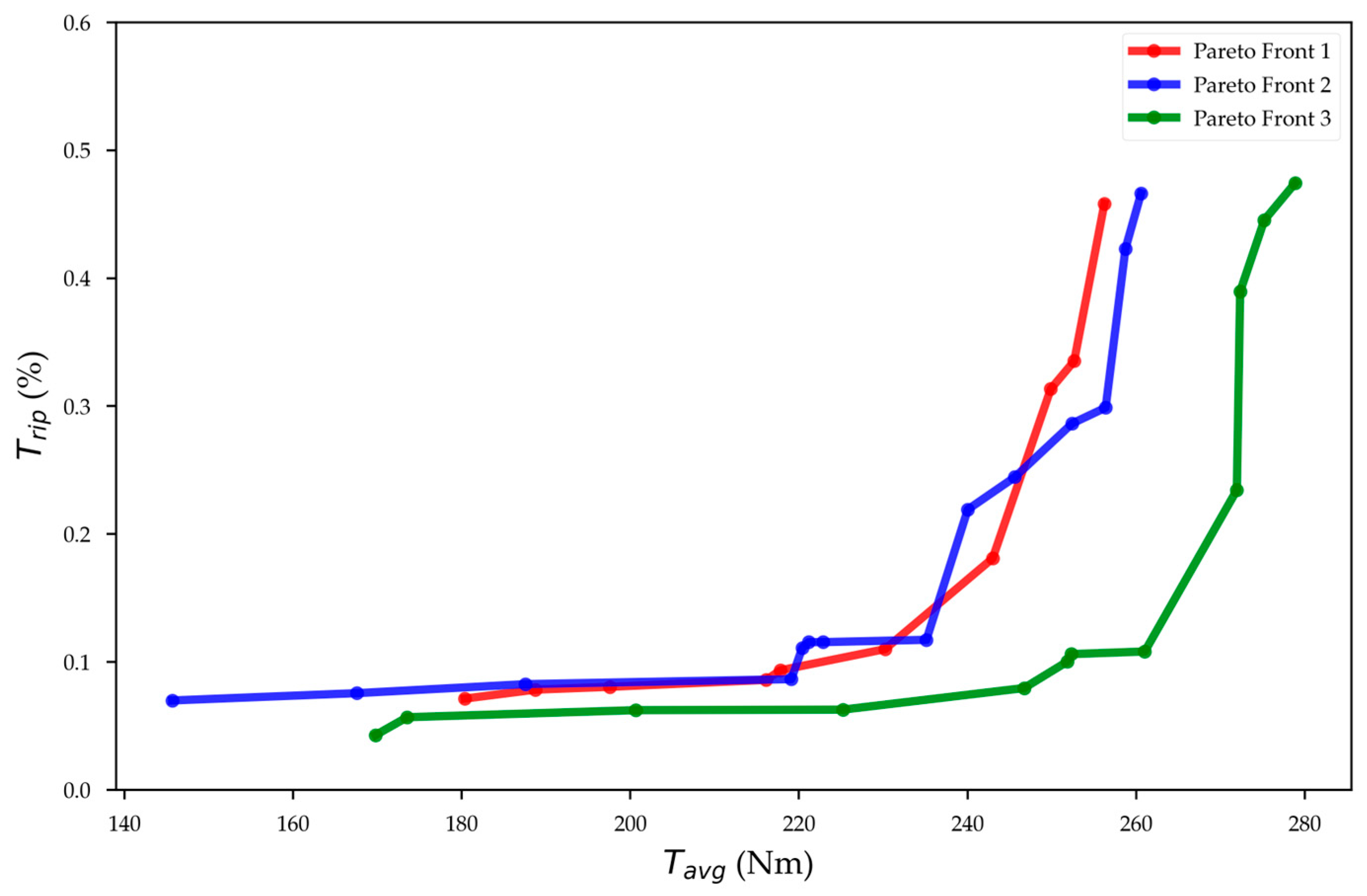
Three different schemes are compared: no filling, Halbach filling, and parallel filling. The conditions for these schemes differ only in whether permanent magnets of ferrite material are included and the magnetizing direction of those magnets. To compare the performance of the three structures and verify whether adding ferrite magnets is effective in improving motor performance, the three structures are modeled, parameterized, and meshed, and boundary conditions are set. The performance of the three different motor structures is obtained using parameter scanning. Specifically, the parameterized parameters are sampled using the Latin hypercube method, which ensures a uniform sampling across the parameter space and helps explore the design space efficiently. Motor performance is then calculated through FEM. The results are depicted in Figure 5. Only the data points on the Pareto front were retained. The Pareto front represents the trade-off curve in the optimization process, capturing the best trade-offs between conflicting objectives.
After conducting simulation tests based on three different magnetization methods, it was found that adding ferrite magnets and adopting parallel magnetization methods can significantly improve the performance of the motor. Simulation results of the three different configurations show that the presence or absence of ferrite magnets has a notable impact on motor performance. The addition of ferrite material contributes to an increase in the average torque of the motor. Specifically, employing the parallel magnetization method leads to a substantial enhancement in average torque compared to both the Halbach and no-ferrite methods, resulting in superior torque ripple performance as well. Notably, with a torque ripple of approximately 10%, the average torque achieved by the parallel magnetization scheme is about 10% higher than that of the other two schemes.

3. Methodology

3.1. Model Design Variables and Optimal Objectives

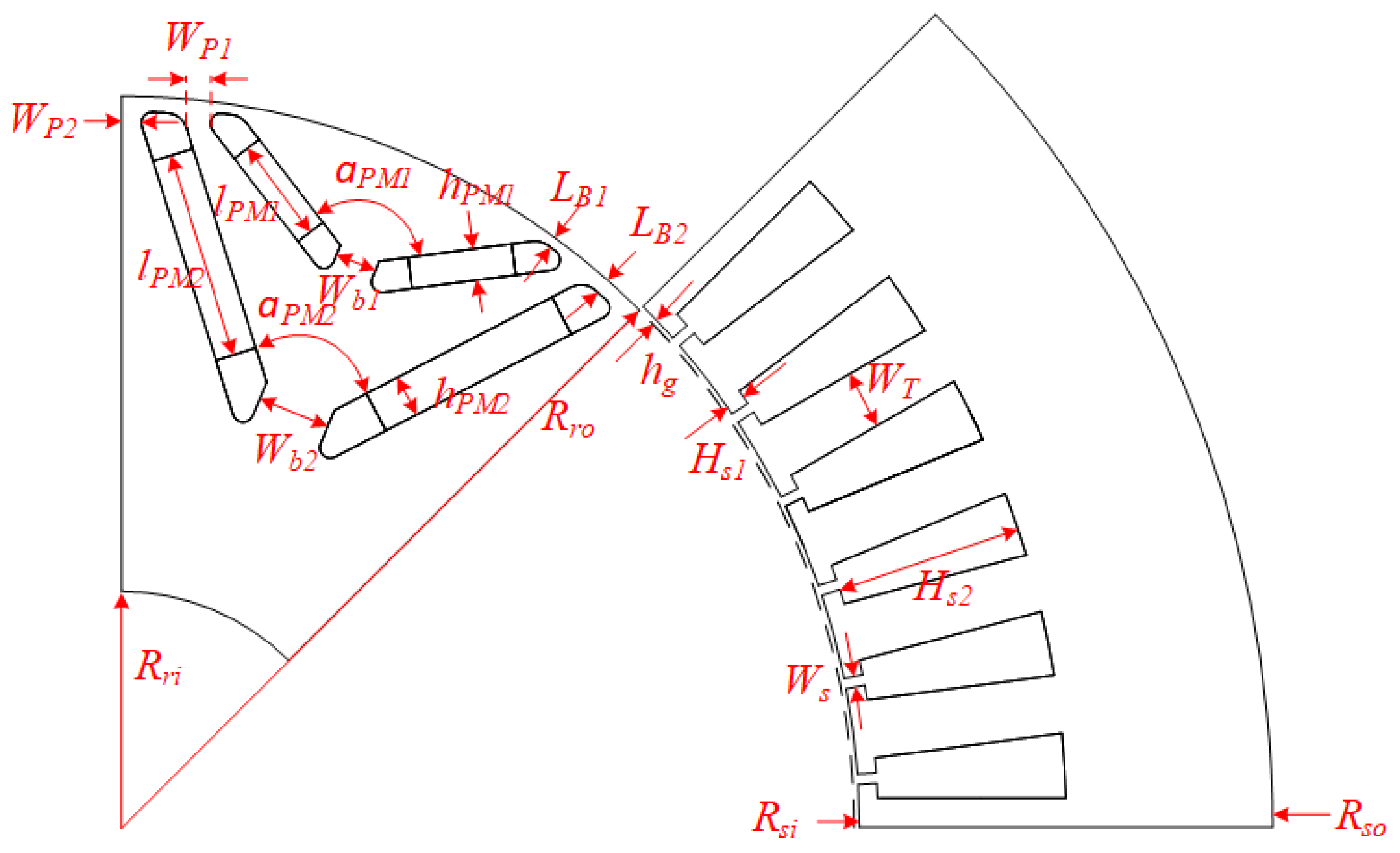
The finite element model of a forty-eight-slot, eight-pole IPMSM with a double-layer V-shaped structure, including NdFeB and ferrite magnets, has been set up in JAMG Designer 22.0.01. The motor model is parameterized, and the results are shown in Figure 6. The parameterization of the model includes both the rotor and stator parts. The motor model can be modified by simply changing the parameter values. Key parts of the motor have been parameterized, such as the stator slot width, slot depth, rotor permanent magnet dimensions, embedding position of the permanent magnets, the angle of the V-shaped permanent magnets, and the width of the magnetic bridge.
As shown in Figure 6 and Table 1, a total of 21 design parameters are included, covering key aspects of the motor’s geometry, materials, and operating conditions. These parameters have been carefully selected to capture the most significant factors affecting motor performance while ensuring computational efficiency. A rationalized parameter range is set to encompass realistic design variations and facilitate comprehensive optimization.
Several parameters are fixed to maintain consistency and practicality in the design process. These include the rotor inner diameter, rotor outer diameter, stator inner diameter, stator outer diameter, and air gap thickness, which are fundamental dimensions critical to motor functionality and manufacturing feasibility.
The multi-objective optimization problem (MOOP) can be described as the problem of finding the optimal solution in the feasible solution set, minimizing all objective functions under the constraints. Here, the goal-designed MOOP has N decision variables and M objective functions. Each decision variable has its upper bound (UB) and lower bound (LB), which can also be viewed as a constraint. If one wishes to maximize some objective function f m x , one can put a negative sign, i.e., f m x , which turns the maximization problem into a minimization problem. The MOOP is governed by (1) and (2).
x i L B x i x i U B , i = 1 , , N ;   x i x = x 1 , , x N
y m = f m x , m = 1 , , M ;   f m x f = f 1 , , f M
Cost serves as an important part of motor design [29]. For the optimization objectives, the optimization objectives set here are average torque, torque ripple, total cost of materials, and weight of the motor. For torque ripple and cost, it is hoped that the smaller, the better, and for the average torque, it is hoped that the larger, the better. It can be represented by the following Formula (3).
min f 1 x = T a v g f 2 x = T r i p f 3 x = C o s t f 4 x = W e i g h t
Since cost calculation is required, an intermediate calculation is required. Table 2 shows the data for the materials used.

3.2. Sampling Method

Sampling in the decision space and evaluating sample performance are crucial tasks in parametric analysis. The quality of sampling strongly influences analysis accuracy, predictive model nature, and final optimization outcomes. Achieving a representative model requires balancing uniformity and dispersion in the sample set. Samples should cover as much decision space as possible while maintaining proximity to each other, avoiding local sparsity or crowding.
Random sampling is a fundamental technique where each sample has an equal chance of selection. It ensures representative samples, making inferential statistics more reliable by reducing bias and facilitating the application of the central limit theorem for estimating probability distributions.
Full factorial sampling considers all combinations of factor levels, revealing interactions between different factors. However, as the number and levels of factors increase, the required number of experiments grows rapidly, rendering full factorial sampling impractical for large-scale problems.
Latin hypercube sampling generates samples in a multidimensional parameter space, aiming to fully explore the entire range of each parameter. Unlike simple random sampling, Latin hypercube sampling stratifies each dimension to ensure more even coverage. This method is particularly useful when computing resources are limited, approximating the effect of full factorial sampling with fewer sample points, especially when variables are relatively independent.
Given the numerous parameters in this model and the characteristics of different sampling methods, the Latin hypercube sampling method is adopted here for its ability to effectively explore parameter space while conserving computational resources.

3.3. Surrogate Model

3.3.1. Model Training Strategy

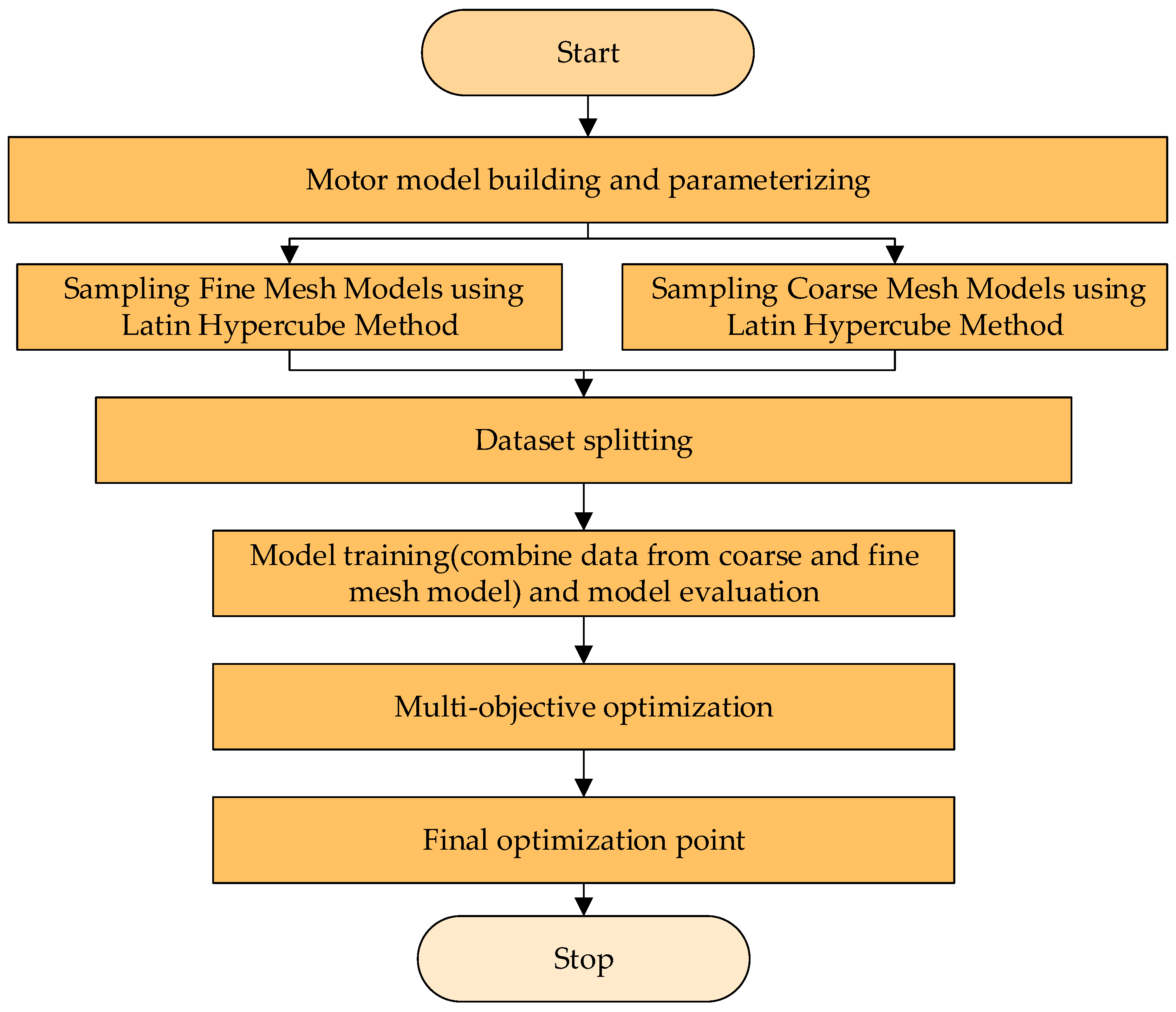
The flow chart of this strategy is shown in Figure 7. The entire strategy starts by creating a finite element model of the motor and parameterizing it. After selecting the parameter variable change space, the design experiment (Latin hypercube sampling) method is used to sample and perform FEA calculations to obtain the dataset. It is worth noting that this strategy simultaneously samples the coarse mesh model and the fine mesh model and uses the data from both to perform model training.

3.3.2. Discussion

There are many methods for constructing surrogate models. Response surface methodology (RSM) is one of the most common algorithms. The general form of a quadratic response surface model is similar to a quadratic linear regression model. By designing experiments, the response between inputs and outputs can be obtained. However, when using the response surface methodology, the number of parameters and objectives for the motor model is very limited. The Kriging model, also known as Gaussian process regression, can provide more accurate predictions. However, the accuracy of the Kriging model largely depends on the correlation between input and output variables, and the computational cost of statistical interpolation methods such as Kriging becomes very high as the amount of input data increases. Machine learning-based methods, such as SVR, can fit more data and more complex nonlinear relationships. Deep learning methods can model a large number of inputs, but obtaining a good model requires a large amount of data. Balancing model accuracy and data volume is a challenge [20].

3.3.3. Model Construction

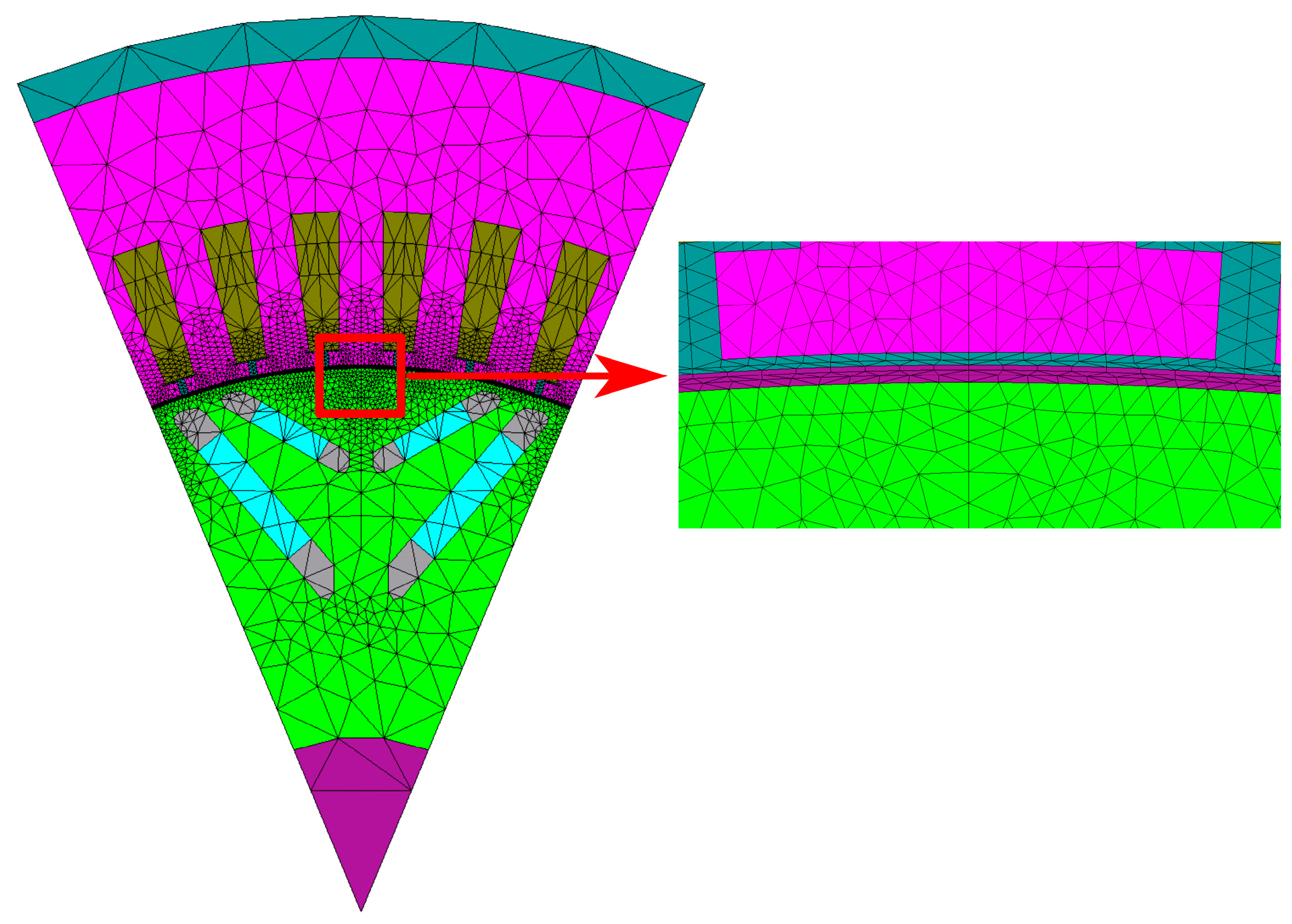
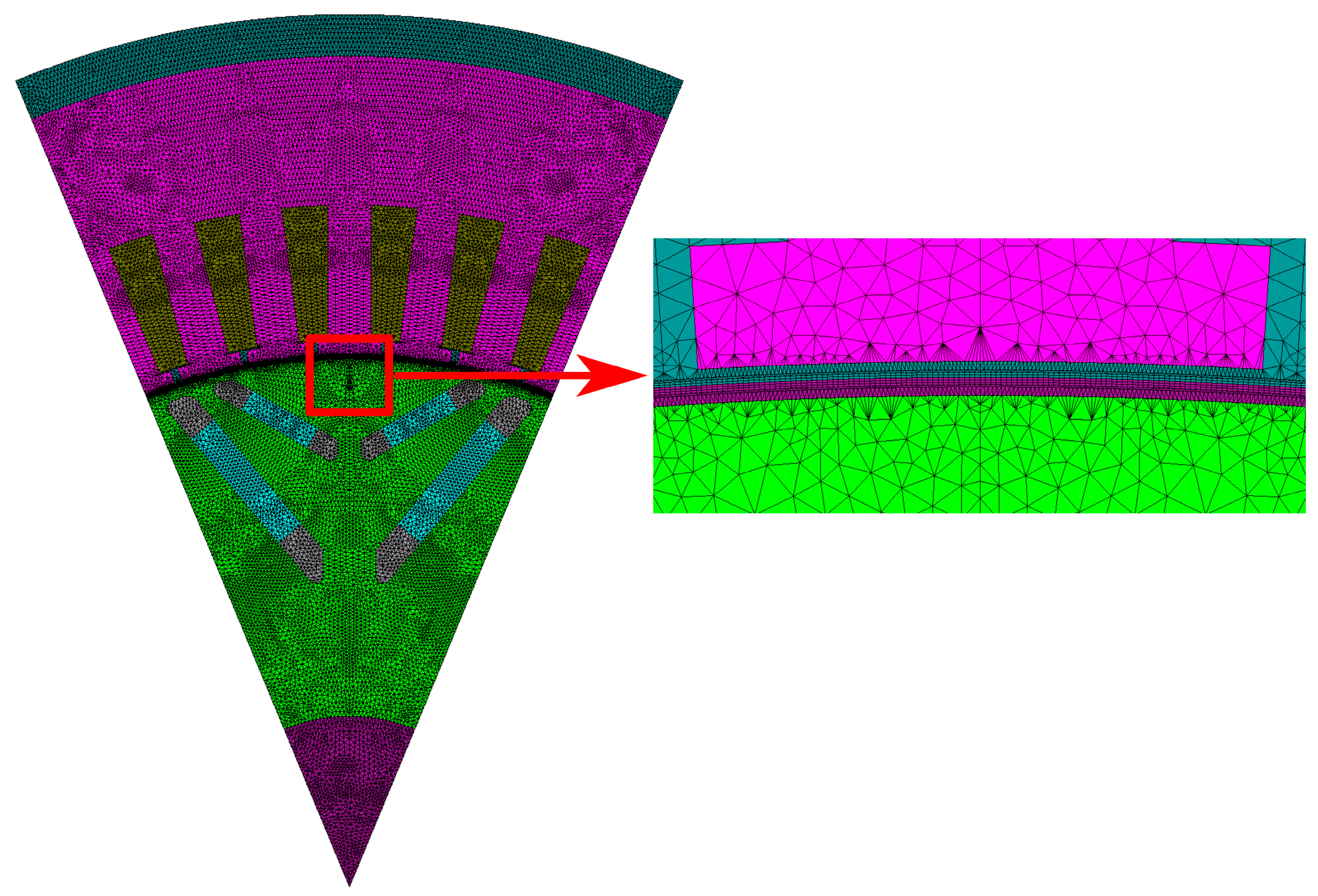
The method used here is to build the model by using a small amount of fine mesh FEA data and a large amount of coarser mesh FEA data, then, based on SVR, train the model by using these two datasets. Figure 8 shows the coarse mesh model; Figure 9 shows the fine mesh model.
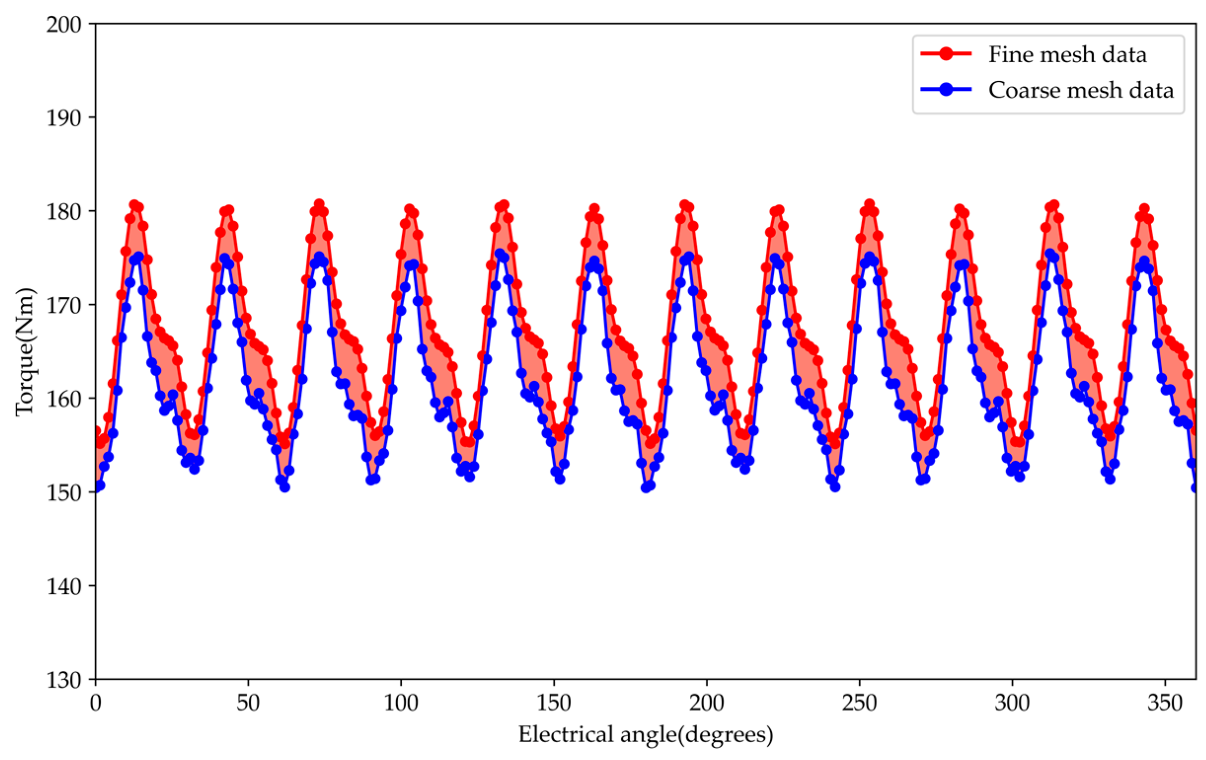
For finite element analysis, the accuracy of its calculation results is related to the precision of mesh division. The finer the mesh division, the more accurate the calculation results are, but at the same time, it also takes longer. Figure 10 shows the average torque data obtained through finite element simulation using the above coarse and fine mesh divisions. The horizontal axis represents the electrical angle, the vertical axis represents the average torque, the red curve represents the fine mesh data, and the blue curve represents the coarse mesh data. The error between the data obtained from the fine mesh and the data obtained from the coarse mesh calculation is shown in Figure 11.
The analysis of the obtained data shows that the torque results calculated using coarse mesh are smaller than those calculated using fine mesh. For the processing of the mesh, the overall refinement of the mesh is increased, especially at the air gap position, and the mesh is divided more finely in the circumferential direction.
For the SVR problem, it can be understood as training and learning a regression model f ( x ) = ω T φ ( x ) + b for a given dataset D = x 1 , y 1 , x 2 , y 2 , , x n , y n . To obtain this, the model needs to satisfy (4) and (5), where ξ i , ξ i * are the slack variables.
min ω , b , ξ , ξ * , E 1 2 ω 2 + C E + ξ i + ξ i *
y i ω T φ x i b E + ξ i ω T φ x i + b y i E + ξ i *
Since this strategy uses two different sets of data to train the same model, the above formulas are no longer used and should satisfy the following Formulas (6) and (7).
min ω t , ω s , b , ξ , ξ * , E 1 2 ω t 2 + ω s 2 + C E + ξ i + ξ i * + λ 2 ω t ω s 2 + b t b s 2
y i ω t T φ x i b E + ξ i ω t T φ x i + b y i E + ξ i * y i ω s T φ x i b E + ξ i ω s T φ x i + b y i E + ξ i *
For the evaluation of the model, two evaluation indicators are used. R-squared (R2) and Root Mean Square Error (RMSE) are two metrics used to assess regression models.
R2 measures how well the model explains the variation of the data. It ranges from 0 to 1, with 1 meaning perfect prediction. A higher R2 indicates a better fit. R2 can be defined as
R 2 = 1 S S r e s S S t o t = 1 i P y i y ^ i 2 i P y i y ¯ i 2
RMSE measures the average error magnitude between the model’s predictions and the actual data. It is given in the same units as the data, and a lower RMSE means a better fit. RMSE can be defined as
R M S E = i P y i y ^ i 2 P
In short, R2 shows the explanatory power of the model, while RMSE shows the error size. To provide a more comprehensive evaluation of the model’s performance, both metrics should be used simultaneously to ensure that the model performs well in terms of explaining data variability and prediction accuracy.
The quality of model training is closely related to the amount of training data. Too few training data can lead to poor model performance, while too many training data can improve the model performance, but they will also consume more time. Therefore, it is necessary to select a training set of appropriate size. The relationship between training data size and model metrics is shown in Figure 12, with the horizontal axis representing the size of the dataset and the vertical axis representing the model evaluation metrics. As the number of training sets increases, the model metrics first increase rapidly, and then even if the number of training sets increases, the model metrics only slowly increase. Considering the time factor, 1500 data points are a viable choice.
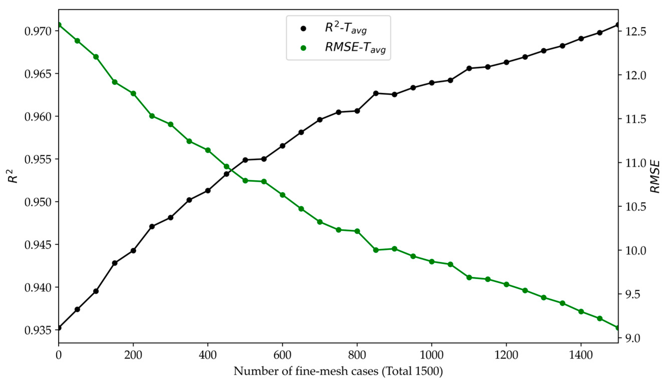
Due to the use of both coarse mesh data and fine mesh data to train the model simultaneously, the proportion of fine mesh data in the total dataset also needs to be considered, as too many fine mesh data will consume more time. As shown in Figure 13, the total amount of data is 1500, with a fine mesh on the horizontal axis. The black curve represents the R2 value, with a larger value being better. The green curve represents the RMSE, with a smaller value being better. Due to the random sampling used in each experiment, the experimental result curve may fluctuate. However, it can be seen from the overall trend that with the increase in fine mesh data, the performance of the model is getting better and better.
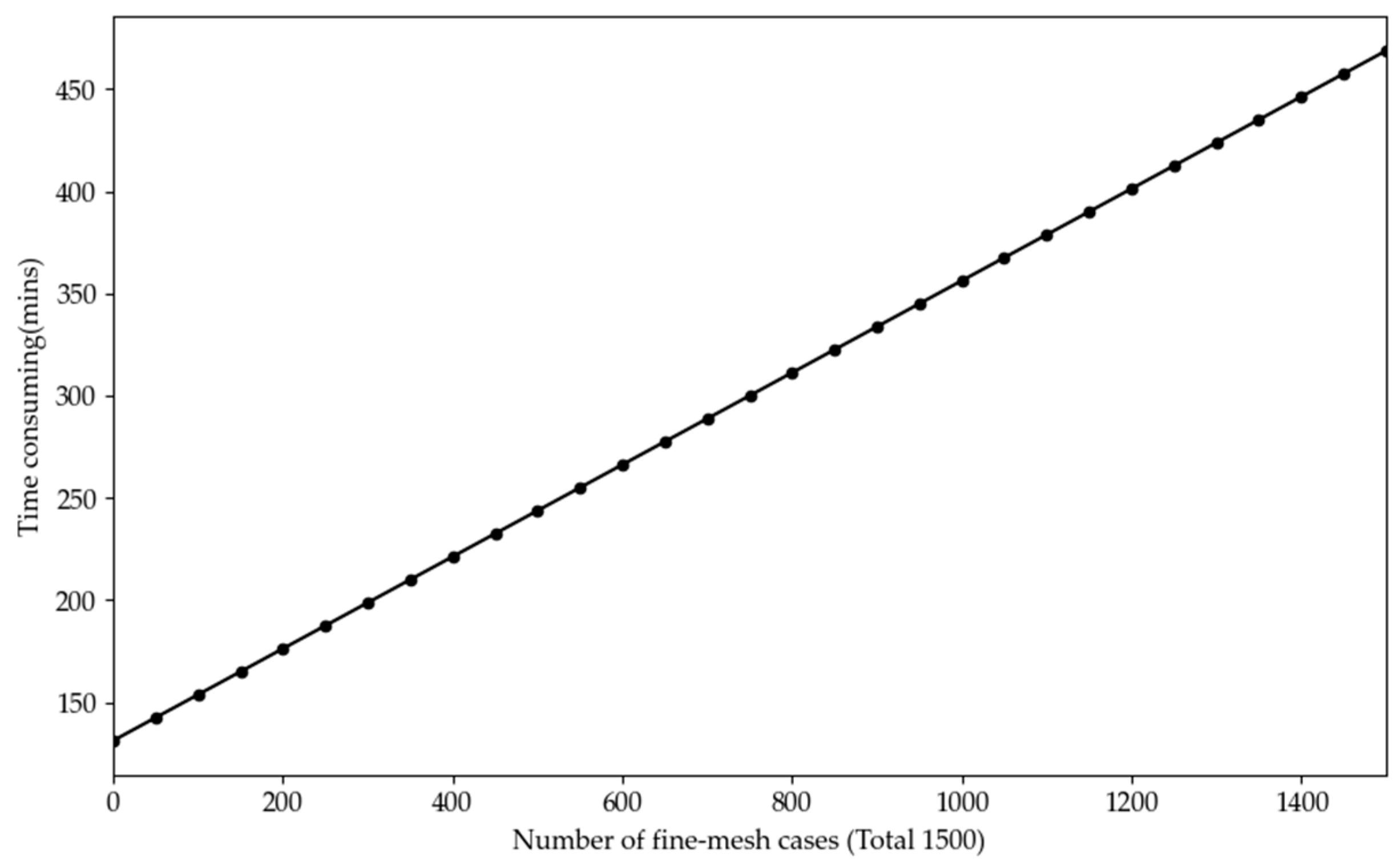
Figure 14 shows the time consumption of different numbers of fine mesh cases. As the number of fine mesh cases increases, the time spent increases linearly. Considering the metrics of the model and the balance of time consumption, 500 fine mesh cases were selected.
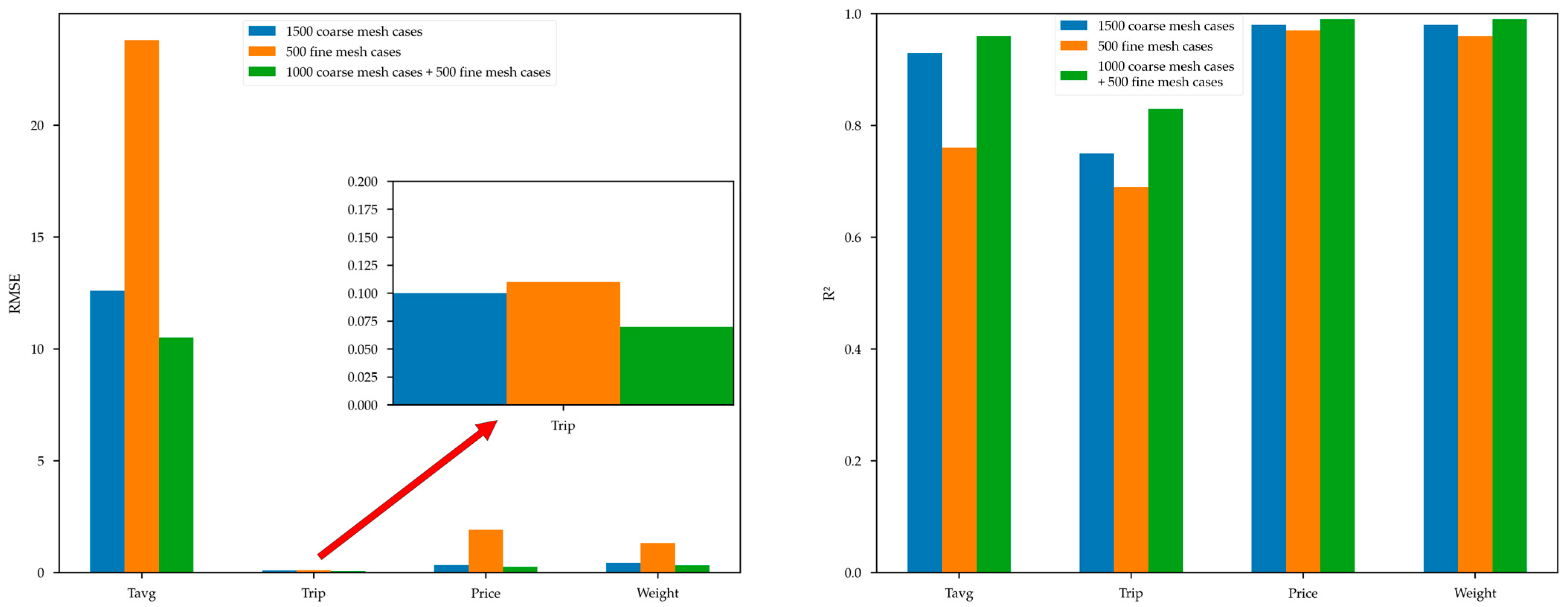
As shown in Figure 15, the evaluation metrics R2 and RMSE of the model trained on three different datasets, namely 1500 coarse mesh data, 500 fine mesh data, and 1000 coarse mesh data + 500 fine mesh data, are plotted. The specific values are shown in Table 3. Among them, the group of 1000 coarse mesh cases + 500 fine mesh cases have better indicators.
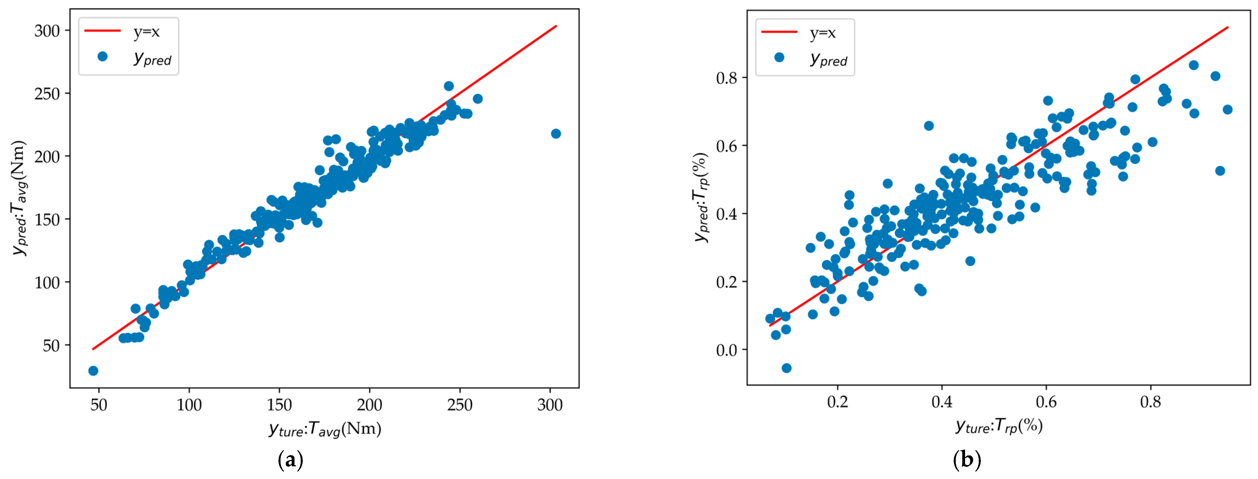
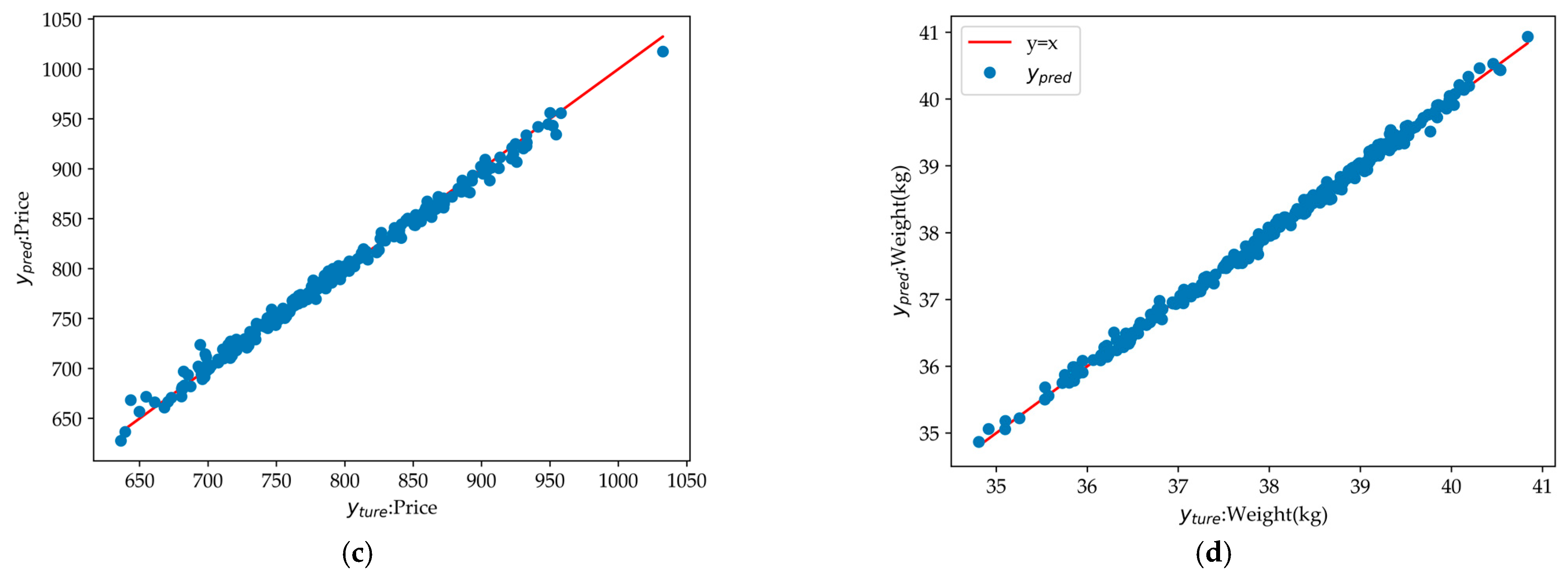
Figure 16 shows charts of the predicted values and actual values of the model trained using the group of 1000 coarse mesh cases + 500 fine mesh cases. In these charts, the information of R2 and RMSE are also shown.

3.3.4. Optimization

The Non-dominated Sorting Genetic Algorithm II (NSGA-II) is a popular multi-objective optimization algorithm used to solve complex optimization problems that have more than one objective to be optimized simultaneously.
NSGA-II addresses some of the main issues found in its predecessor, NSGA, by introducing a fast non-dominated sorting approach, a crowding distance assignment mechanism, and an elitist selection strategy. The fast non-dominated sorting approach categorizes the population into different levels or fronts based on the dominance relation, where the first front is completely non-dominated and subsequent fronts have increasing levels of dominance.
The crowding distance is a measure of how close an individual is to its neighbors. A larger crowding distance means a solution is better because it signifies a less crowded region in the objective space, which encourages diversity in the solutions.
The selection strategy in NSGA-II ensures that the best solutions are carried over to the next generation, promoting the retention of high-quality solutions.
NSGA-II is widely used in various fields, such as engineering design, where trade-offs between conflicting objectives are common. Its ability to find a set of diverse and high-quality Pareto-optimal solutions, which represent the best possible trade-offs, makes it a powerful tool for multi-objective optimization problems.

3.3.5. Results

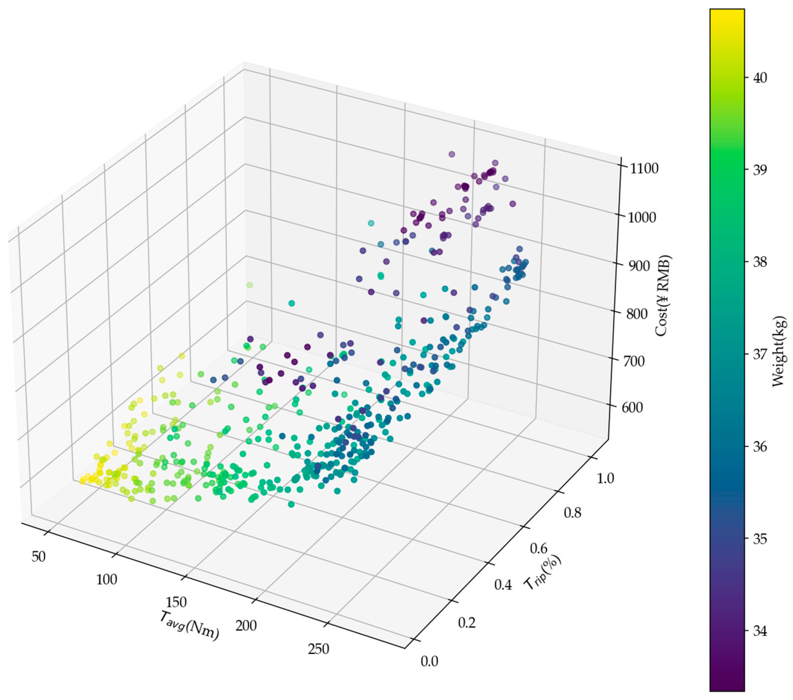
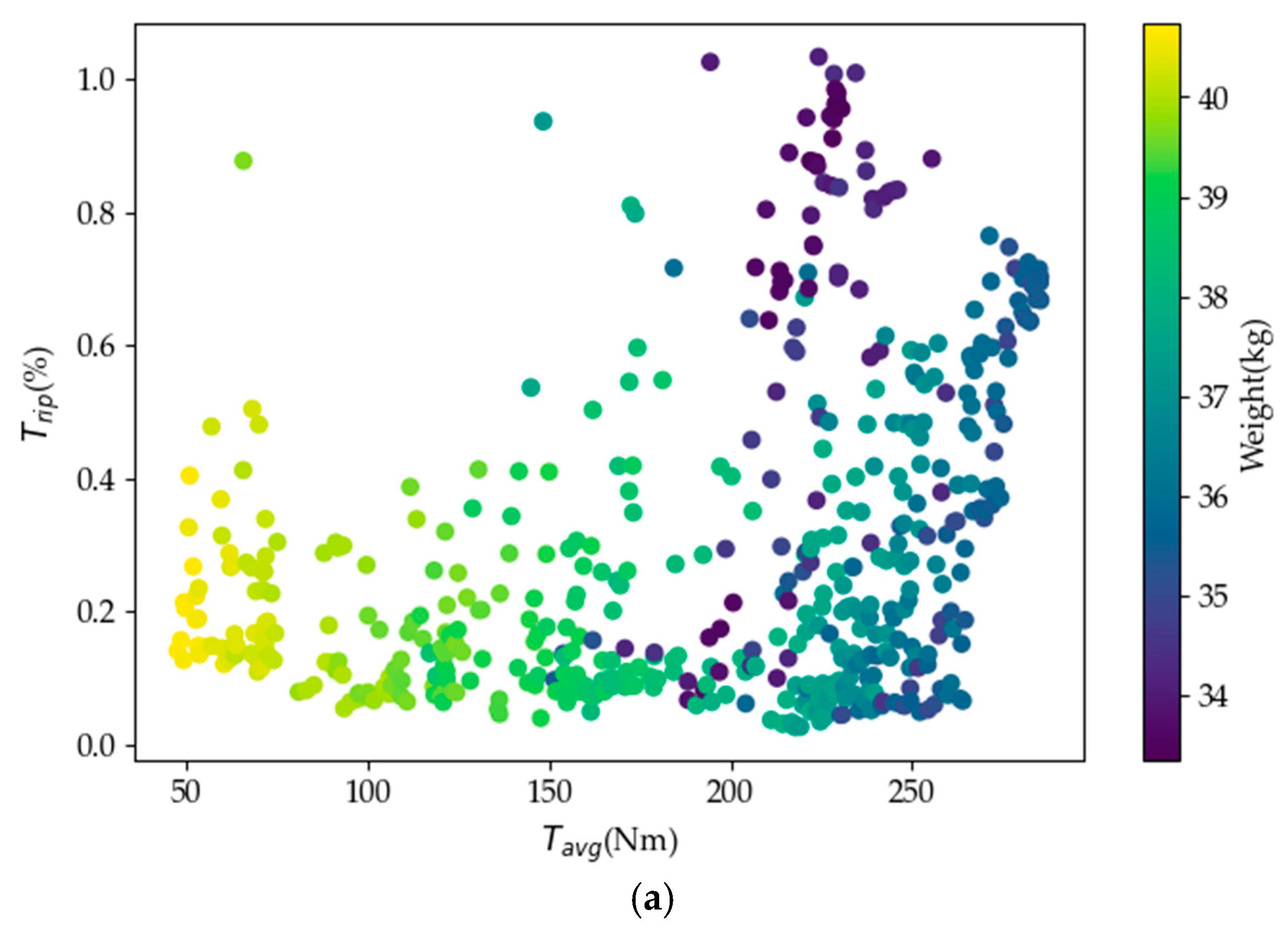
The optimized results are plotted, as shown in Figure 17. It shows the Pareto solution results. Figure 18 shows the pairwise relationship between each target value.
Table 4 gives the initial parameters and initial performance of the motor, as well as the optimal parameters and motor performance based on the finite element algorithm and this algorithm. Through comparison, it is found that both the finite element algorithm and this algorithm can significantly improve motor performance. At the same time, the motor performance obtained by the finite element algorithm and this algorithm is similar, which proves that this algorithm has good accuracy.
The reduced calculation burden by the proposed strategy is verified in this section. First, the specifications of the CPU for testing different strategies are given in Table 5. The unit has 32 processors for the parallel evaluation of cases and has a frequency of 2400 MHz. Model sampling and finite element calculations take a lot of time, but since the experiment is designed using sampling, parallel computing can be used to calculate several results at the same time. The model fitting and validation phase is fast, taking only about 10 min. In the subsequent optimization phase, the agent model can search for the optimal results for 10,000 cases in just 10 min. On the other hand, optimization based on direct FEA requires approximately 70 h to observe the Pareto front for more than 5000 cases. In summary, this strategy finds a more complete frontier more efficiently than the traditional counterparts.

4. Conclusions

This paper compares the performance of motors without adding ferrite magnets, adding ferrite magnets in a Halbach arrangement, and adding ferrite magnets in a parallel arrangement. It was found that adding ferrite magnets and arranging them in parallel significantly improved motor performance. Under the same torque pulsation condition, the parallel magnetization structure has a 10% improvement in torque compared with the other two structures.
And the method of combining coarse mesh finite element data and fine mesh finite element data is used to establish a surrogate model and perform multi-objective optimization of the motor, which can greatly reduce the calculation time while obtaining good accuracy, saving 94% the computational burden compared with high-fidelity FEA. The method of combining coarse mesh data and fine mesh data to train a surrogate model can improve the accuracy of the model compared to the method of using a single type of data. The R2 value of the torque model increased from 0.93 (1500 coarse mesh cases) and 0.76 (500 fine mesh cases) to 0.96, and the RMSE decreased from 12.6 (1500 coarse mesh cases) and 13.8 (500 fine mesh cases) to 10.5. At the same time, the optimal result predicted by the surrogate model is brought into the FEA software (JMAG-Designer 22.0.01) for verification. The final accuracy error between the predicted values and the FEA calculation results is less than 1%.
Future research may focus on the further development of surrogate models based on machine learning, particularly exploring the application of artificial neural networks (ANNs) in motor design and investigating the feasibility of methods such as convolutional neural networks (CNNs), generative adversarial networks (GANs), and Kolmogorov–Arnold networks (KANs), etc. Balancing data volume and model accuracy is also a critical issue. To standardize the evaluation of different models, there is an urgent need to establish a benchmark testing system. Additionally, developing more universal strategies to adapt to different motor structures will be a key area of focus.

Author Contributions

ConceptualizIation, S.G. and H.Z.; methodology, S.G.; software (JMAG-Designer 22.0.01), S.G.; validation, S.G. and X.S.; formal analysis, S.G.; investigation, S.G.; resources, S.G.; data curation, H.Z.; writing—original draft preparation, S.G.; writing—review and editing, X.S.; visualization, S.G.; supervision, H.Z.; project administration, H.Z.; funding acquisition, H.Z. All authors have read and agreed to the published version of the manuscript.

Funding

This work is supported by the Guangzhou-HKUST (GZ) Joint Funding Program (No. 2023A03J0102), the Guangdong Basic and Applied Basic Research Foundation (No. 2022A1515110361), and the Guangdong Basic and Applied Basic Research Foundation (No. 2024A1515010882).

Data Availability Statement

The data presented in this study are available on request from the corresponding author.

Conflicts of Interest

The authors declare no conflicts of interest.

References

  1. Kurian, A.G.; Thakur, S.K.; Kunde, S.; Sankpal, K.; Wagh, S. Challenges in Electric Vehicle NVH. In Proceedings of the 2021 IEEE Transportation Electrification Conference (ITEC-India), New Delhi, India, 16–19 December 2021. [Google Scholar]
  2. Hu, Y.; Wang, Z.; Li, X. Impact of policies on electric vehicle diffusion: An evolutionary game of small world network analysis. J. Clean. Prod. 2020, 265, 121703. [Google Scholar] [CrossRef]
  3. Kaarlela, T.; Villagrossi, E.; Rastegarpanah, A.; San-Miguel-Tello, A.; Pitkäaho, T. Robotised disassembly of electric vehicle batteries: A systematic literature review. J. Manuf. Syst. 2024, 74, 901–921. [Google Scholar] [CrossRef]
  4. Malozyomov, B.V.; Martyushev, N.V.; Kukartsev, V.A.; Kukartsev, V.V.; Tynchenko, S.V.; Klyuev, R.V.; Zagorodnii, N.A.; Tynchenko, Y.A. Study of Supercapacitors Built in the Start-Up System of the Main Diesel Locomotive. Energies 2023, 16, 3909. [Google Scholar] [CrossRef]
  5. Zhao, N.; Schofield, N. An Induction Machine Design With Parameter Optimization for a 120-kW Electric Vehicle. IEEE Trans. Transp. Electrif. 2020, 6, 592–601. [Google Scholar] [CrossRef]
  6. Dianati, B.; Kahourzade, S.; Mahmoudi, A. Optimization of Axial-Flux Induction Motors for the Application of Electric Vehicles Considering Driving Cycles. IEEE Trans. Energy Convers. 2020, 35, 1522–1533. [Google Scholar] [CrossRef]
  7. Guan, Y.; Zhu, Z.Q.; Afinowi, I.A.A.; Mipo, J.C.; Farah, P. Design of synchronous reluctance and permanent magnet synchronous reluctance machines for electric vehicle application. In Proceedings of the 2014 17th International Conference on Electrical Machines and Systems (ICEMS), Hangzhou, China, 22–25 October 2014; pp. 1853–1859. [Google Scholar]
  8. Credo, A.; Fabri, G.; Villani, M.; Popescu, M. Adopting the Topology Optimization in the Design of High-Speed Synchronous Reluctance Motors for Electric Vehicles. IEEE Trans. Ind. Appl. 2020, 56, 5429–5438. [Google Scholar] [CrossRef]
  9. Nardo, M.D.; Calzo, G.L.; Galea, M.; Gerada, C. Design Optimization of a High-Speed Synchronous Reluctance Machine. IEEE Trans. Ind. Appl. 2018, 54, 233–243. [Google Scholar] [CrossRef]
  10. Jeong, C.-L.; Kim, Y.-K.; Hur, J. Optimized Design of PMSM With Hybrid-Type Permanent Magnet for Improving Performance and Reliability. IEEE Trans. Ind. Appl. 2019, 55, 4692–4701. [Google Scholar] [CrossRef]
  11. Sun, X.; Shi, Z.; Lei, G.; Guo, Y.; Zhu, J. Multi-Objective Design Optimization of an IPMSM Based on Multilevel Strategy. IEEE Trans. Ind. Electron. 2021, 68, 139–148. [Google Scholar] [CrossRef]
  12. Cho, S.-K.; Jung, K.-H.; Choi, J.-Y. Design Optimization of Interior Permanent Magnet Synchronous Motor for Electric Compressors of Air-Conditioning Systems Mounted on EVs and HEVs. IEEE Trans. Magn. 2018, 54, 8204705. [Google Scholar] [CrossRef]
  13. Jung, J.-W.; Lee, S.-H.; Lee, G.-H.; Hong, J.-P.; Lee, D.-H.; Kim, K.-N. Reduction Design of Vibration and Noise in IPMSM Type Integrated Starter and Generator for HEV. IEEE Trans. Magn. 2010, 46, 2454–2457. [Google Scholar] [CrossRef]
  14. Zhao, H.; Liu, C.; Dong, Z.; Huang, R.; Li, X. Design and Optimization of a Magnetic-Geared Direct-Drive Machine With V-Shaped Permanent Magnets for Ship Propulsion. IEEE Trans. Transp. Electrif. 2022, 8, 1619–1633. [Google Scholar] [CrossRef]
  15. Li, X.; Wei, Z.; Zhao, Y.; Wang, X.; Hua, W. Design and Analysis of Surface-Mounted Permanent-Magnet Field-Modulation Machine for Achieving High Power Factor. IEEE Trans. Ind. Electron. 2024, 71, 4375–4386. [Google Scholar] [CrossRef]
  16. Zhu, X.; Wu, W.; Quan, L.; Xiang, Z.; Gu, W. Design and Multi-Objective Stratified Optimization of a Less-Rare-Earth Hybrid Permanent Magnets Motor With High Torque Density and Low Cost. IEEE Trans. Energy Convers. 2019, 34, 1178–1189. [Google Scholar] [CrossRef]
  17. Zhao, H.; Liu, C.; Song, Z.; Wang, W. Exact Modeling and Multiobjective Optimization of Vernier Machines. IEEE Trans. Ind. Electron. 2021, 68, 11740–11751. [Google Scholar] [CrossRef]
  18. Liu, C.; Chau, K.T.; Lee, C.H.T.; Song, Z. A Critical Review of Advanced Electric Machines and Control Strategies for Electric Vehicles. Proc. IEEE 2021, 109, 1004–1028. [Google Scholar] [CrossRef]
  19. Hwang, C.C.; Cho, Y.H. Effects of leakage flux on magnetic fields of interior permanent magnet synchronous motors. IEEE Trans. Magn. 2001, 37, 3021–3024. [Google Scholar] [CrossRef]
  20. Cheng, M.; Zhao, X.; Dhimish, M.; Qiu, W.; Niu, S. A Review of Data-driven Surrogate Models for Design Optimization of Electric Motors. IEEE Trans. Transp. Electrif. 2024. [Google Scholar] [CrossRef]
  21. Ren, Z.; Ma, J.; Qi, Y.; Zhang, D.; Koh, C.S. Managing Uncertainties of Permanent Magnet Synchronous Machine by Adaptive Kriging Assisted Weight Index Monte Carlo Simulation Method. IEEE Trans. Energy Convers. 2020, 35, 2162–2169. [Google Scholar] [CrossRef]
  22. Zhang, Z.; Rao, S.; Zhang, X. Performance Prediction of Switched Reluctance Motor Using Improved Generalized Regression Neural Networks for Design Optimization. CES Trans. Electr. Mach. Syst. 2018, 2, 371–376. [Google Scholar] [CrossRef]
  23. Dhulipati, H.; Ghosh, E.; Mukundan, S.; Korta, P.; Tjong, J.; Kar, N.C. Advanced Design Optimization Technique for Torque Profile Improvement in Six-Phase PMSM Using Supervised Machine Learning for Direct-Drive EV. IEEE Trans. Energy Convers. 2019, 34, 2041–2051. [Google Scholar] [CrossRef]
  24. Raia, M.R.; Ruba, M.; Nemes, R.O.; Martis, C. Artificial Neural Network and Data Dimensionality Reduction Based on Machine Learning Methods for PMSM Model Order Reduction. IEEE Access 2021, 9, 102345–102354. [Google Scholar] [CrossRef]
  25. Demir, U.; Akgun, G.; Akuner, M.C.; Pourkarimi, M.; Akgun, O.; Akinci, T.C. An Innovative Approach to Electrical Motor Geometry Generation Using Machine Learning and Image Processing Techniques. IEEE Access 2023, 11, 48651–48666. [Google Scholar] [CrossRef]
  26. Dlala, E. Hybrid Rotor Assembly. US20200412190A1, 31 December 2020. [Google Scholar]
  27. Liu, K.; Yin, M.; Hua, W.; Ma, Z.; Lin, M.; Kong, Y. Design and Analysis of Halbach Ironless Flywheel BLDC Motor/Generators. IEEE Trans. Magn. 2018, 54, 8109305. [Google Scholar] [CrossRef]
  28. Wang, X.; Wu, L.; Zhou, S.; Hu, C.; Zhao, M. Optimization Design of In-wheel Motor Based on Halbach (Ce,Nd)FeB Magnet. In Proceedings of the 2019 22nd International Conference on Electrical Machines and Systems (ICEMS), Harbin, China, 11–14 August 2019; pp. 1–4. [Google Scholar]
  29. Yu, J.; Liu, C.; Liu, S.; Zhao, H. Comparative Study of Double-Stator Interior-PM Vernier Machines Based on Electromagnetic-Structural Coupling Analysis. IEEE Trans. Ind. Electron. 2021, 68, 10510–10520. [Google Scholar] [CrossRef]
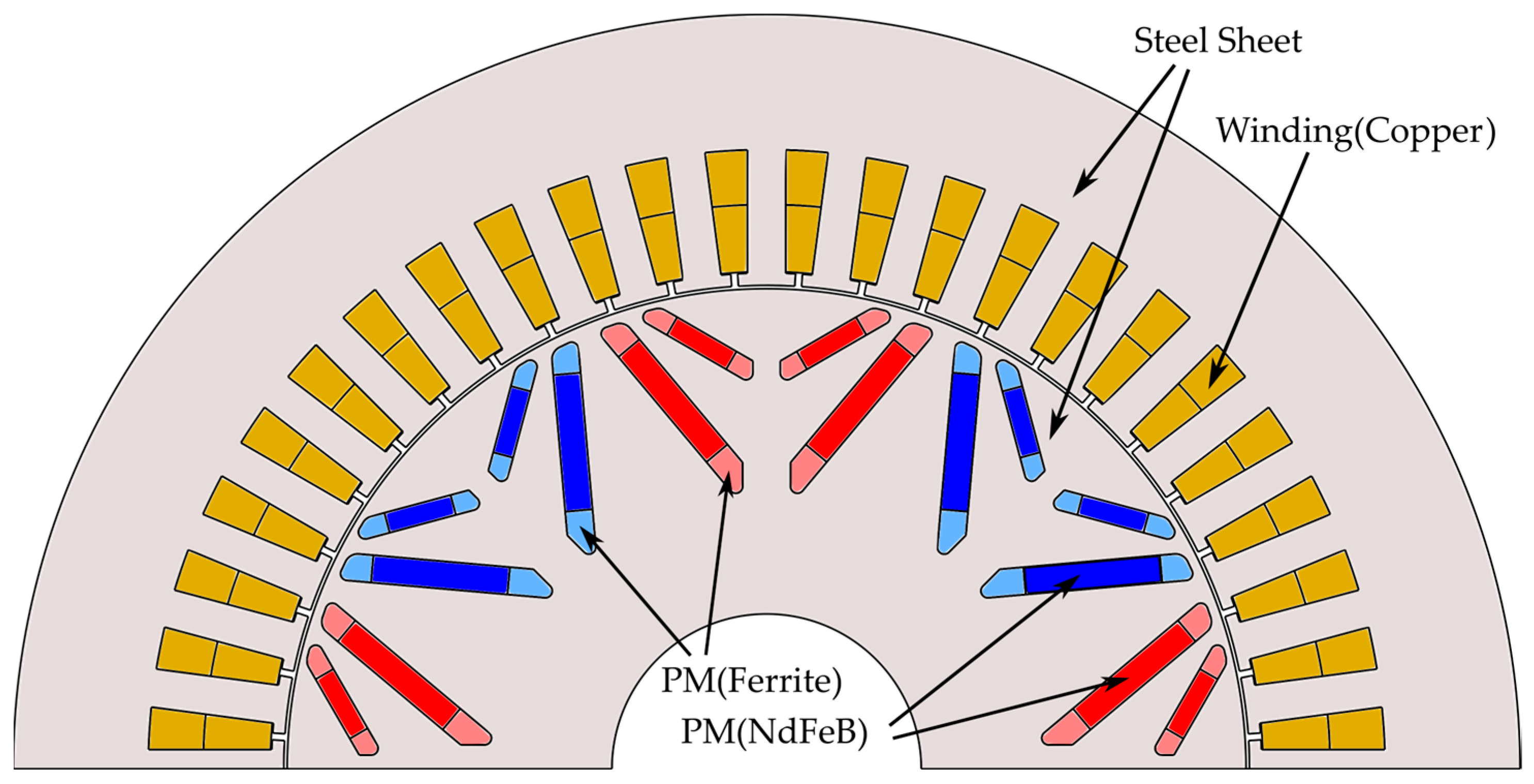
Figure 1. Target PMSM structure (sectional view).
Energies 17 03864 g001
Figure 2. Three different structures. Air (a): No ferrite magnets, only air in the slots. Halbach (b): Ferrite magnets with Halbach arrangement. Parallel (c): Ferrite magnets with parallel arrangement, aligned with NdFeB.
Energies 17 03864 g002
Figure 3. The magnetic flux density contour plots of the three structures. Air (a): No ferrite magnets, only air in the slots. Halbach (b): Ferrite magnets with Halbach arrangement. Parallel (c): Ferrite magnets with parallel arrangement, aligned with NdFeB.
Energies 17 03864 g003
Figure 4. The air gap magnetic flux density diagrams of the three structures.
Energies 17 03864 g004
Figure 5. Pareto front results on average torque and torque ripple after parameter scanning of three different structures. Pareto front 1: Result of structure with no ferrite magnets, only air in the slots. Pareto front 2: Result of structure with ferrite magnets in Halbach arrangement. Pareto front 3: Result of structure with ferrite magnets in parallel arrangement.
Energies 17 03864 g005
Figure 6. Parameterized model of the studied IPMSM.
Energies 17 03864 g006
Figure 7. Flowchart of the full process.
Energies 17 03864 g007
Figure 8. Coarse mesh model.
Energies 17 03864 g008
Figure 9. Fine mesh model.
Energies 17 03864 g009
Figure 10. Torque of fine mesh data and coarse mesh data.
Energies 17 03864 g010
Figure 11. Error of fine mesh data minus coarse mesh data.
Energies 17 03864 g011
Figure 12. Sample size and the validation metrics R2.
Energies 17 03864 g012
Figure 13. Validation metrics R2 and the number of fine mesh cases.
Energies 17 03864 g013
Figure 14. Time consumption of different numbers of fine mesh cases (total 1500 cases).
Energies 17 03864 g014
Figure 15. Validation metrics R2 and RMSE in three conditions.
Energies 17 03864 g015
Figure 16. R2 and RMSE charts. (a): Graph of predicted and actual average torque values; (b): Graph of predicted and actual torque ripple values; (c): Graph of predicted and actual cost values; (d): Graph of predicted and actual mass (weight) values.
Energies 17 03864 g016aEnergies 17 03864 g016b
Figure 17. The Pareto front chart obtained by using the surrogate model and optimization algorithm.
Energies 17 03864 g017
Figure 18. Pareto front of three objectives in the subspace view. (a): Trip–Tavg–Weight; (b): Cost–Tavg–Weight; (c): Cost–Trip–Weight.
Energies 17 03864 g018aEnergies 17 03864 g018b
Table 1. Design parameters, description, and range or value.
Design ParametersUnitDescriptionRange/Value
RrimmRotor inner radius23
RrommRotor outer radius70
RsimmStator inner radius70.5
RsommStator outer radius110
hgmmAir gap length0.5
WTmmTooth width2–8
WsmmSlot opening width1–4
Hs1mmSlot opening depth0–5
Hs2mmSlot depth15–25
lPM1mmPM1 length8–10
lPM2mmPM2 length15–18
hPM1mmPM1 height3–5
hPM2mmPM2 height3–5
LB1mmBridge length1–2
LB2mmBridge length1–2
WP1mmPM Web width1–2
WP2mmPM Web width1–2.5
Wb1mmMagnet post width2–3
Wb2mmMagnet post width3–7
αPM1degPM1 V shape angle110–135
αPM2degPM2 V shape angle70–110
Table 2. Material information.
MaterialDensity (kg/m3)Cost (RMB/kg)
N50-NdFeb7500229.460
Steel-50CS100078505.050
Copper896070.700
Ferrite50003.715
Table 3. Validation metrics R2 and RMSE.
Groupf(x)RMSER2
1500 coarse mesh casesTavg12.60.93
Trip0.100.75
Cost0.330.98
Weight0.430.98
500 fine mesh casesTavg23.80.76
Trip0.110.69
Cost1.920.97
Weight1.320.96
1000 coarse mesh cases + 500 fine mesh casesTavg10.50.96
Trip0.070.83
Cost0.260.99
Weight0.320.99
Table 4. Optimal results. FEA vs. surrogate model.
ParametersInitial DesignFinal Optimized by FEA MethodFinal Optimized by Surrogate MethodFinite Element Verification CalculationUnit
Design variablesWT5.63.693.063.06mm
Ws11.731.331.33mm
Hs11.81.843.393.39mm
Hs21824.9217.8417.84mm
lPM1109.929.949.94mm
lPM22015.3217.3617.36mm
hPM133.413.873.87mm
hPM244.114.264.26mm
LB111.351.131.13mm
LB21.51.671.821.82mm
WP11.51.081.661.66mm
WP21.51.241.731.73mm
Wb132.122.462.46mm
Wb275.623.663.66mm
αPM1120121.22129.41129.41deg
αPM28077.81101.47101.47deg
ObjectivesTage169.49271.25(1 60.03%)270.52(↑59.61%)271.13Nm
Trip17.1610.36(2 39.62%)9.23(↓46.21%)9.08%
Cost793.64772.12(↓2.71%)782.34(↓1.42%)782.50RMB
Weight39.1436.73(↓6.15%)35.99(↓7.99%)36.12kg
1 ↑ means that this indicator is improved compared with the initial design indicator. 2 ↓ means that this indicator is decreased compared with the initial design indicator.
Table 5. Time spent for calculations.
Optimization StrategyCPU TypeTime Spent for StepTotal Time Consumed
Proposed methodIntel core i9-13980hx (Intel, Santa Clara, CA, USA) @2400 MHz 24 Cores with 32 Processors1. Case evaluation by FEA 1000 + 500 = 1500 cases (4 h)
2. Model construction and fitting (10 min)
3. Using NSGA-II solve MOOP and find the Pareto frontier, 10,000 cases (10 min)
4.2 h
FEA-based optimizationDirect global optimization by NSGA-II, 5000 cases70 h
Disclaimer/Publisher’s Note: The statements, opinions and data contained in all publications are solely those of the individual author(s) and contributor(s) and not of MDPI and/or the editor(s). MDPI and/or the editor(s) disclaim responsibility for any injury to people or property resulting from any ideas, methods, instructions or products referred to in the content.