Estimation of Railway Line Impedance at Low Frequency Using Onboard Measurements Only

Abstract

Estimating line impedance is relevant in transmission and distribution networks, in particular for planning and control. The large number of deployed PMUs has fostered the use of passive indirect methods based on network model identification. Electrified railways are a particular example of a distribution network, with moving highly dynamic loads, that would benefit from line impedance information for energy efficiency and optimization purposes, but for which many of the methods used in industrial applications cannot be directly applied. The estimate is carried out onboard using a passive method in a single-point perspective, suitable for implementation with energy metering onboard equipment. A comparison of two methods is carried out based on the non-linear least mean squares (LMS) optimization of an over-determined system of equations and on the auto- and cross-spectra of the pantograph voltage and current. The methods are checked preliminarily with a simulated synthetic network, showing good accuracy, within 5%. They are then applied to measured data over a 20 min run over the Swiss $16.7$ Hz railway network. Both methods are suitable to track network impedance in real time during the train journey; but with suitable checks on the significance of the pantograph current and on the values of the coefficient of determination, the LMS method seems more reliable with predictable behavior.

1. Introduction

Power system analysis is extensively used for planning, protection, and control of power systems. Among the various components of a power system, transmission or distribution lines require accurate and correct estimates of parameters for a wide range of tasks: power flow calculations (including harmonic power flow), state estimation and fault identification, supporting grid analysis, dispatching, control, optimization, and energy efficiency improvement.

Focusing on the general panorama of electrified guideway transport, real-time information on the electrical parameters of traction lines is particularly useful: on the one hand, to further refine and improve the accuracy of energy optimization algorithms [1,2,3] and the prediction of system receptivity and efficiency (such as the influence of line voltage drops [4]), as well as, on the other hand, to support various types of protection methods [5,6]. It is briefly recalled that although the return circuit of electrified railways (the so-called “cold path”) has significant variability, caused by the electrical properties of the rails and their connection [7], the overall loop impedance we are focusing on is mainly determined by the geometry of the line conductors and the electrical characteristics of connected power supply items. For clarity, a graphical description is provided with two simplified schemes of the overall distribution of the traction power supply of a $16.7$ Hz single-phase system (see Figure 1a) and of hot and cold paths (see Figure 1b).

In general, transmission line circuits are considered constant for both per-unit-length parameters (quite obvious if minor changes due to, e.g., temperature, are neglected) and the resulting line section parameters. This allows the determination of parameters by offline methods, assuming they are unchanged for a long time.

Two approaches may be identified that interact quite differently with the infrastructure subject to investigation:

• First, analytical expressions [10,11] or numerical methods [12] using material and geometrical data; in this case, consolidated expressions are used (e.g., Carson’s equations [10]) starting from accurate and/or conservative estimates of conductors’ geometry and data; geometry changes are mainly due to the transition from open-air to tunnel sections, as considered in [11,13].
• Second, more accurately relying on measurement results, using for example volt-amperometric, reflectometry or bridge methods (the former being best suited for industrial environments and, in particular, railways); the measured data are then used to fit a predetermined model, for instance, of the type used in the first approach above. Examples are the RL model fitted in [14] by means of a recursive model identification algorithm based on a quadratic cost function; and [15], by means of a Kalman filter. Other methods are, for example, volt-amperometric and vector network analyzer (reflectometric) methods for grid impedance measurement, including power converters [16,17].

These methods are in general best applicable when the lines are out of service, although online measurements are possible by suitably coupled instruments at substations [18,19,20].

Assuming constant parameters, however, represents an approximation, not only for electrified transport but also for industrial transmission and distribution networks themselves. First of all, the temperature affects the resistance of both overhead and cable lines, and also the capacitance for the latter. Inductance is also affected to a minor extent due to the change in length of conductors and consequential sagging [21]. Aging of materials also exerts some influence and slowly affects their electrical properties [22,23]. In addition, smaller loads and devices attached in the middle of long line sections may be assimilated to an overall slight change in line properties. For industrial networks there is also the possibility of the switching on and off of loads and entire secondary branches, as well as reactive power compensation devices (such as capacitor banks). All these factors cause random fluctuations in parameters with different dynamics.

The most promising approaches to an online estimate of equivalent line parameters are based on supervisory control and data acquisition (SCADA) measurements, and then, improving in quality and accuracy, on the newer phasor measuring units (PMUs) [24,25], providing real-time high-quality voltage and current synchrophasors. These techniques, however, are expensive and in general not suitable for a dynamic scenario such as electrified railways, where the loads move along the network, thus being constantly reconfigured. PMUs would be in principle deployed on rolling stock and at TPSs, that should share a common protocol and synchronization; at the moment measuring units onboard rolling stock are targeted to energy consumption and fundamental quantities only [26,27], and have a low-pace synchronization, for example, by means of a GSM connection. Furthermore, loads feature a significant dynamic behavior (passing often from power absorption during traction to power delivery during regenerative braking) and a complex harmonic signature, depending on the loading level, on operating conditions, and on the instantaneous amount of auxiliaries onboard [28,29,30].

For railway applications there is no standardized approach to network monitoring. The normative requirements are limited to the installation onboard rolling stock of energy metering units, implementing the requirements of the EN 50463-2 [31] with single-point metering [32]. Other specific monitoring devices are installed for signaling protection, by monitoring some current harmonics for abnormally large intensity.

The focus is thus on the exploitation of data coming from passive listening at the pantograph interface, in order to determine the line impedance behavior at low frequency, to support power and energy forecasting and optimization [26,32]. The estimate of the traction line impedance at the pantograph interface in real time is by itself novel, and the use of passive listening using only local electrical quantities adds additional novelty.

The structure of the paper is as follows. The first section (Section 2) classifies and discusses the methods for line parameter estimation, identifying limitations and advantages, in the perspective of a later implementation onboard rolling stock for use in electrified railways with the aim of energy consumption optimization. Section 3 clarifies the proposed method as an improvement of existing models, considering the constraints of the onboard implementation and the exigency of a simple and robust method. Section 5.1 provides details of the implementation, specifying, for example, the model order, the number of samples considered for each estimate, and, in general, the equations that make up the proposed model. Section 4 shows simulation results for a preliminary verification and assessment of the behavior and accuracy of the two proposed algorithms under controlled conditions. Section 5, finally, provides results based on experimental data for a reference case of a $16.7$ Hz railway, for which extensive experimental data are available [33]. Conclusions are drawn in Section 6 together with a discussion of future improvements to the method to extend it to harmonic frequencies, to exploit specific information (e.g., when the grid voltage is accessible at ideally no-load conditions with zero current absorption), and to apply it to other cases, such as distribution grids, having chosen an electrified railway line as a challenging reference case with moving dynamic loads.

2. Existing Methods for Line Parameter Estimation

Methods for the estimation of line parameters may be divided into active and passive methods. In [14], a further distinction is made, introducing quasi-passive methods, without discussing them further, in addition to defining them as “combining the advantages of active and passive methods”.

• Active methods inject an excitation signal to probe network impedance by measuring voltage and current during the excitation and soon after that. Excitation signals have been extensively analyzed and optimized for frequency spectrum coverage and reconstruction performance, or, in other words, achievable frequency resolution and signal-to-noise ratio [34,35].
• Passive methods exploit existing measured quantities, passively listening to the network. Several signal characteristics have been considered to maximize detectability, such as using traveling waves generated by disturbances to obtain the line propagation constant [36]. In general, the focus is on numerical methods for reduction of indeterminacy and improvement of the signal-to-noise ratio by exploiting an increased number of measurements (e.g., using least mean squares, Lagrangian multipliers, Kalman filter, empirical weighting criteria [15,37,38,39]).

Active methods are not suitable for direct implementation onboard rolling stock (differently manufactured and owned), but deployment at substations would be possible, provided that the impact on safety and availability, in addition to cost and maintenance, is assessed and accepted. An example can be found in [35], where a butterfly-type converter (employing only two IGBTs and four diodes) generates the test signals with a chirp PWM (pulse-width modulation) method, scanning the frequency range up to about 5 kHz. A similar system was used in [40] for the determination in live conditions of the resonance frequency of a 25 kV railway line: the converter architecture in this case was based on stacked full IGBT H-bridges.

In general, passive methods are preferable, especially considering the possible integration of the estimation function in existing hardware, that is nowadays being installed onboard for power quality monitoring and energy metering purposes [31,32]. Differently from distribution and transmission networks, railways in general do not have PMUs installed, at least in a sufficiently large number.

A promising approach for passive methods is applying advanced techniques for model identification using models that are sufficiently accurate for the purpose. At low frequency, an R-L model is acceptable and simpler; such models have also been used for sophisticated methods, such as in [15], where they claim that system resonances occur at very high frequency, in reality limiting its applicability. While assuming resonances at high frequency may indeed be reasonable for small networks (e.g., smart and micro grids), it is not for railways, with resonances between tens of Hz and a few kHz at most.

• For DC railways the first line resonance is mainly determined by the interaction with the traction power station (TPS), and, in particular, with the output resonant filter [41]; resonances at higher frequency are related to the catenary distribution system and can be predicted by transmission line theory [41,42]. Other resonant circuits can be identified in the input filters onboard locomotives, showing a very low resonance frequency, on the order of 10 Hz to 20 Hz [43]; more complex oscillation patterns, also related to the position of the train along the line, may take place, as extensively investigated in [44].
• For AC railways substations generally do not contain filters and the main line resonance is located at higher frequency, on the order of about 1 or a few kHz for 25 kV systems [35,45,46], which have shorter supply sections than $16.7$ Hz systems [8,47].

The basic approach of passive methods exploits measurements taken with the same network topology and electrical characteristics, but in two different supply conditions. Ideally the flowing current is measured after an instantaneous change in the supply voltage. This method has found extensive application in smart grids [14,15,48], using known equations for a “reference state” and a “perturbed state”.

3. Proposed Methods for Line Impedance Estimation

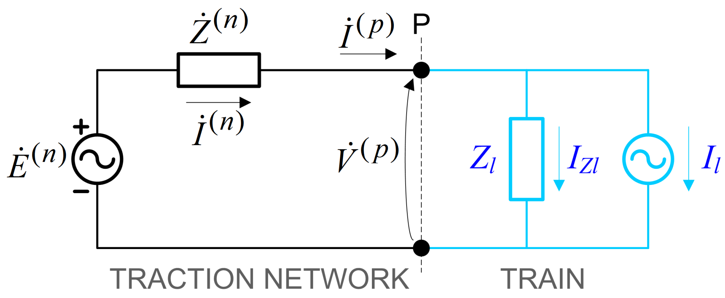
For railways the measurement point is the pantograph with current and voltage, $I_p$ and $V_p$, respectively. In contrast to a meshed distribution network, but similar to a transmission network, a railway traction line is locally one-dimensional, with a loose meshed architecture, with branching lines conveniently separated by several km. Conversely, quite peculiarly, loads distributed along the line that move and vary at a variable pace (depending on speed and operating profile) are characterized by significant dynamics and periodically become sources during regenerative braking. The network seen at the pantograph can be represented by the equivalent Thevenin circuit $V_n$ and $Z_n$. The train load may be represented by its equivalent Norton circuit, $Z_l$ and $I_l$, that for the present method is not relevant (and for this reason it is in light blue color in Figure 2, where the equivalent circuit is shown).

For power load flow and power consumption studies of electrified railways only the fundamental is relevant with good approximation, as is commonplace [27] and demonstrated in [49]. By neglecting harmonic components and focusing on the fundamental component the overall error in the active power estimate was shown to be less than 1% [49]. For this reason all quantities are assumed at the fundamental only.

The following is the Kirchhoff law equation for the black part of the circuit (left of pantograph), using subscripts “n” and “p” for network and pantograph, respectively. The representation is adjusted and simplified, so that $\angle I_p=0$ and it is used as a reference and all other phase angles are expressed with respect to it [3].

$$E_n\angle {\theta }_n=Z_n\angle {\xi }_n{I}_p\angle 0+V_p\angle {\varphi }_p$$

(1)

The same expression can be written repeatedly for a sequence of measurements $m=1,2,\dots M$ of the phasor quantities separated by a time step $\delta t$ (that to fix ideas may correspond to the fundamental period, i.e., $\delta t=T$), with the overall duration of the measurements being $T_m=M\delta t$. For compactness, the subscript is replaced with m, referring to the measurement number, and dropping the reference to the network and pantograph (that remain clear having selected different letters for the quantities). This formulation has been proposed in the past a few times, like in [50,51], both of which use a direct approach, with one based on differences between two states of the system; both are considered and discussed in the following.

By assuming that the instantaneous network frequency does not change significantly across adjacent measurements (spanning in total $T_m$ seconds) and, similarly, that the parameters of the network may be assumed constant in this time interval, the solution of the equations can be attempted by building an over-determined system of equations. The assumption of steady network parameters corresponds to assuming that in the time span $T_m$ the position of the train is unchanged, as it is for the other trains within the same supply section, as they also contribute, although only marginally at the fundamental and low-order harmonics, to the network impedance $Z_n$ values, as seen from the pantograph of the train under study.

3.1. Method Based on Least Mean Squares Solution of Over-Determined System

This method is implicitly based on the assumption that a perturbed state is available for the network, and this is ensured by the multitude of loads running on the supply section and by the disturbance originating from the upstream network. Equation (1) can be replicated for the M time steps as

$$\begin{array}{cc}\hfill E_1\angle {\theta }_1& =Z_1\angle {\xi }_1{I}_1\angle 0+V_1\angle {\varphi }_1\hfill \\ \hfill E_2\angle {\theta }_2& =Z_2\angle {\xi }_2{I}_2\angle 0+V_2\angle {\varphi }_2\hfill \\ \hfill & ⋮\hfill \\ \hfill E_M\angle {\theta }_M& =Z_M\angle {\xi }_M{I}_M\angle 0+V_M\angle {\varphi }_M\hfill \end{array}$$

(2)

This set of equations can be rearranged then in a more compact matrix notation that is used in the following. The solution exploits redundancy.

Phasors V and I are those available from measurements and lead to the estimates of the unknowns E and Z. The quantities in the equations below are complex vectors (with real and imaginary parts) made of M successive measurements and noted in bold. A system with $M>4$ is over-determined and in principle there is no exact solution. Practically speaking, variability and measurement errors require that the system of equations is written with a “nearly equal” sign, and then, the error $\epsilon$ between the measured and reconstructed values is isolated.

$$\mathbf{E}=\mathbf{Z}\mathbf{I}+\mathbf{V}\mathbf{E}-\mathbf{Z}\mathbf{I}-\mathbf{V}=\mathit{\epsilon }$$

(3)

The higher the value of M, the more accurate the solution, although the used number of fundamental periods is larger, thus introducing two sources of variability:

• The spanned position along the line over one solution interval is longer, causing a more evident change in $Z_n$, as the tapping point P moves; the equations of the ideal dependency on the train position are summarized in [8] for two configurations, accounting for supply from one or two TPSs;
• The electrical behavior of rolling stock along the line section becomes more variable and the assumption of a steady operating mode over the interval $T_m$ becomes more inconsistent, with more significant variations in the absorbed power and instantaneous input admittance.

This part is discussed later in Section 5 with the help of experimental data.

This method is similar to what was proposed in [52], where a three-point method and a multi-point method were discussed, with a solution that made use of closed-form expressions for the real and imaginary parts of the network impedance, rather than the more flexible least mean squares approach used here and discussed in Section 5.1. Also, in [52], the necessity of “constant” parameters for the grid was postulated, but the relationship between the sampling time instants was not made clear, nor was the behavior assessed with the increase in the number of sampling periods fed to the algorithm.

It is briefly noted that the system may be replicated for each frequency of interest, other than the fundamental. However, the phasor equations at different frequencies are in reality not independent, since the estimated $Z_n$ values for each frequency must be physically feasible, in agreement with the expected line impedance behavior [8,35,41,45]. This introduces an additional constraint, as the equations to solve for each frequency at each step are in reality coupled by the physical feasibility requisite. As anticipated, for electromechanical simulation purposes and for energy management and optimization, the information on the impedance values at the fundamental only is sufficient.

For the LMS method, the initially used algorithm is the non-linear least mean squares curve fit Matlab function lsqcurvefit(), feeding it with suitable lower and upper bounds, that are never approached by the algorithm, providing a first demonstration of the feasibility of the technique in the various operating conditions and scenarios considered in the examples in Section 5.

The observed deterioration in the quality of the $Z_n$ estimate for time intervals where the absorbed current is very small led to applying the exclusion of such intervals from the LMS estimate. The results are discussed in Section 5.

3.2. Method Based on Auto- and Cross-Spectra

An alternative method for the impedance estimate is that of exploiting the auto-spectrum and cross-spectrum of the pantograph electrical quantities $V_p$ and $I_p$, that we call in the following the auto- and cross-spectrum (ACS) method. This method has been proposed in the literature through the years for various applications, such as, for example, in [53] for general application to control systems, Ref. [54] for impedance spectroscopy of batteries, Ref. [16] for harmonic impedance in distribution grids, and Ref. [43] for estimating the high-frequency line impedance of DC railways.

This technique is normally used over an extended frequency range and not only at the fundamental, using robust techniques for the estimate of the auto- and cross-spectra such as the Welch method [55]. A similar approach may be applied to the present case, by taking the DFT of successive signal segments over the considered time length $T_m$ and limiting the analysis to a few frequency bins around the fundamental or to the fundamental only.

In general, the impedance of a dipole where the voltage V and current I are known may be calculated as

$$\widehat{Z}={\displaystyle \frac{S(I,V)}{S(I,I)}}$$

(4)

having noted with $S$ the generic spectrum, and in particular with $S(I,I)$ the auto-spectrum of I and with $S(I,V)$ the cross-spectrum between I and V.

With the considerations in [16] and observing Figure 2, it is clear that the sought network impedance $Z_n$ cannot result from the direct application of (4) to $V_p$ and $I_p$, as the quantity $E_n$ plays a role. Instead, we are looking at an excitation coming from the right-hand side (the rolling stock) that is able to excite the network impedance, neglecting the assumed-almost-constant $E_n$ contribution. With this aim it is sufficient to take the difference between successive complex phasors of $V_p$ and $I_p$ as resulting from the sliding DFTs; a k-window distance is indicated in [16] for generality, resulting in phasors’ difference vectors located at $kT$ time distance. The indication of “k” in the formulas below is kept for generality; in agreement with the comment in section 3.5 of [16], to limit the phase errors in the two $\Delta$ quantities the distance in time is kept to the minimum allowed by the calculation of the voltage and current FFTs $V_t\left(f\right)$ and $I_t\left(f\right)$. As in Section 3.1 above, the subscript “p” is removed for simplicity and the subscript now indicates the quantity time.

$$\Delta V_t=V_t-V_{t-kT}\Delta I_t=I_t-I_{t-kT}$$

(5)

resulting in two $\Delta$ quantities for voltage and current at time t, that remove constant terms (so largely $E_n$ for our assumption, which will be verified by means of the coherence function values) and focus on the short-term changes exciting the network. As explained later in Section 5, the k value is kept to the minimum number of the periods of the signals taken for one FFT $N_{per}$, which will be shown in the following to be equal to 3.

Based on this, the estimate of the network impedance over time, ${\widehat{Z}}_n\left(t\right)$, is achieved by the auto- and cross-spectra of the pantograph quantities under the assumptions that are discussed in more detail in the following.

$${\widehat{Z}}_n\left(t\right)={\displaystyle \frac{{\left[S(\Delta I_t,\Delta V_t)\right]}^2}{S(\Delta I_t,\Delta I_t)}}$$

(6)

Borkowski [16] provides an interesting discussion of the various cases where a change may occur on the network side or load (rolling stock) side, which can be summarized in the following cases:

• $\Delta E_t=0$, $\Delta I_{l,t}=0$: In this case, no perturbed state is available and the network impedance cannot be estimated;
• $\Delta E_t=0$, $\Delta I_{l,t}\ne 0$: This is the case of interest where the network is “quiet” and the excitation comes from the rolling stock side;
• $\Delta E_t\ne 0$, $\Delta I_{l,t}=0$: In this case, the network has voltage variations, but the rolling stock side does not; this is the case, for example, in standstill or coasting, where power absorption by the rolling stock is minimal, and this is discarded by setting a threshold of significance on the $I_p$ current amplitude;
• $\Delta E_t\ne 0$, $\Delta I_{l,t}\ne 0$: This case is similar to case 2, where changes to the network voltage cannot be excluded; this is the general case that cannot be excluded, but whose occurrence can be minimized by taking a sufficiently small time horizon, as already mentioned for the LMS algorithm and the value of M; in the end any change in E represents a disturbance.

Considering a wide range of external disturbances (noise) and violations of assumptions, we are interested in assessing the quality of the results by exploiting the available quantities. Following the four cases above it is observed that when the changes in the rolling stock current are correlated to those of the pantograph voltage it means that the network voltage changes $\Delta E$ are negligible, leading to isolate case 2. More considerations on this can be found in [16].

With this aim, the coherence function [16,53,54,56] plays an important role:

$$\widehat{C}\left(t\right)={\displaystyle \frac{{\left[S(\Delta I_t,\Delta V_t)\right]}^2}{S(\Delta I_t,\Delta I_t)S(\Delta V_t,\Delta V_t)}}$$

(7)

for which low values going to 0 indicate lack of coherence, and thus, a less reliable estimate of ${\widehat{Z}}_n$; conversely, large $\widehat{C}$ values close to unity confirm a reliable estimate of ${\widehat{Z}}_n$, based on the coherent spectrum components of $I_p\left(f\right)$ and $V_p\left(f\right)$.

The uncertainty in the method was evaluated in [57], as the variance of the local ${\widehat{Z}}_n$ estimate, providing the expression

$$u\left\{{\widehat{Z}}_n\right\}=\sqrt{|{\widehat{Z}}_n{|}^2{\displaystyle \frac{1-\widehat{C}{\left(t\right)}^2}{\widehat{C}{\left(t\right)}^2}}}$$

(8)

${\widehat{Z}}_n$ is a doubly non-central F distribution [53,57] that approximates a normal distribution as long as the number of observed samples is large (this, it is noted, is opposite to the requirement of keeping the rolling stock operating conditions stationary). To this aim, two values for the number of samples are considered in the Results section, corresponding to the number of collected squared FFTs of the two quantities, to apply the Welch algorithm.

The underlying assumptions are that the (i) input and output noise is independent of the input and output signals and that (ii) the correlation length of the noise is shorter than the observed period. Assumption (i) can be challenging if, from a harmonic impedance perspective, grid harmonic terms are considered that may be significantly correlated; whereas assumption (ii) is usually satisfied [57]. It is underlined, however, that in the present case (i) is also satisfied, focusing on the fundamental only and with any correlation with the grid voltage already being embedded in the model of the problem (3).

Also, for the ACS method a sliding approach is applied, calculating the estimate of both the auto- and cross-spectra $S(I_t,I_t)$, $S(V_t,V_t)$, and $S(I_t,V_t)$ by means of the original Bartlett method [53,58], rather than the Welch method [53,55], for the following reason: the calculation is performed on the already-transformed sequences, since on them the $\Delta$ quantities of (5) are calculated as phasor differences. So the moving average of a sequence of sliding squared Fourier transforms as in (6) is calculated iteratively.

As noted in [43], the use of the Bartlett or Welch methods, in case of a reduced number of samples and due to the averaging, reduces the frequency resolution of the estimate. In the present case, focusing on the low-frequency impedance behavior, this is not an issue. On the contrary, in [43] the method was used to estimate the line impedance in the tens of $\mathrm{kHz}$ range, as excited by pantograph electric arcs (excitation by transients), with issues of limited sampling frequency.

A certain number $N_W$ of contiguous Fourier transforms is collected to feed the Bartlett algorithm that simply calculates the auto- and cross-spectra as

$$\widehat{S}(X,X)={\displaystyle \frac{1}{N_W}}\sum _{n=1}^{N_W}|X_n{|}^2\widehat{S}(X,Y)={\displaystyle \frac{1}{N_W}}\sum _{n=1}^{N_W}|X_n||Y_n|$$

(9)

where with the notation “X” and “Y” the previous $\Delta$ quantities are generically indicated in any combination.

4. Preliminary Verification with Synthetic Data

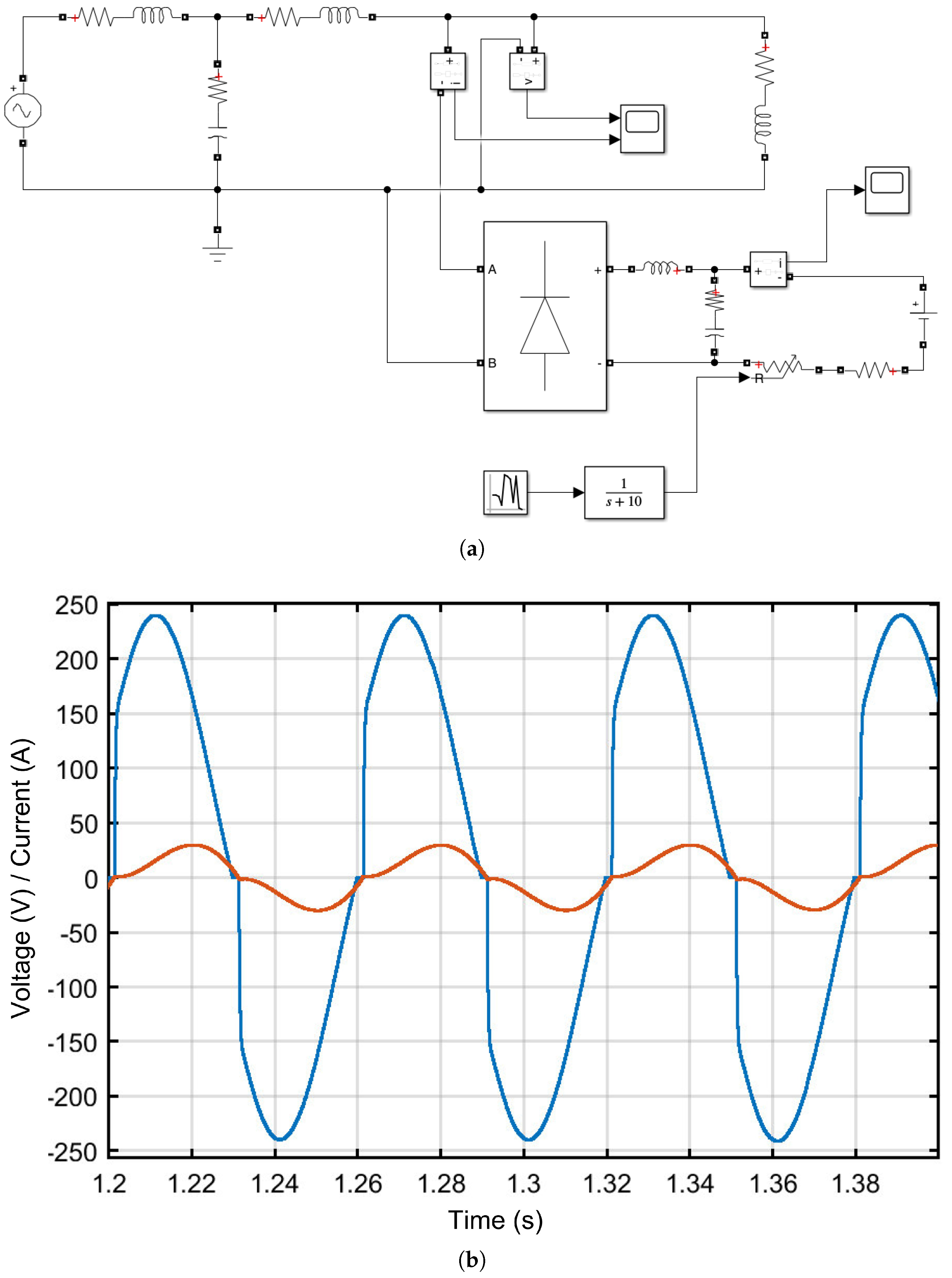
A simple network was created in Matlab Simulink, using the Simscape library, with the purpose of testing the two algorithms under controlled conditions. The network impedance was fixed, but the load was a distorting single-phase diode rectifier, whose power absorption was randomly varied by about $\pm 10\%$. The scheme and the waveforms at the connection point of the distorting load are shown in Figure 3. It is observed that the fundamental frequency was chosen as $16.7$ Hz, although the nominal voltage was then 230 V, but this did not affect the approach and results.

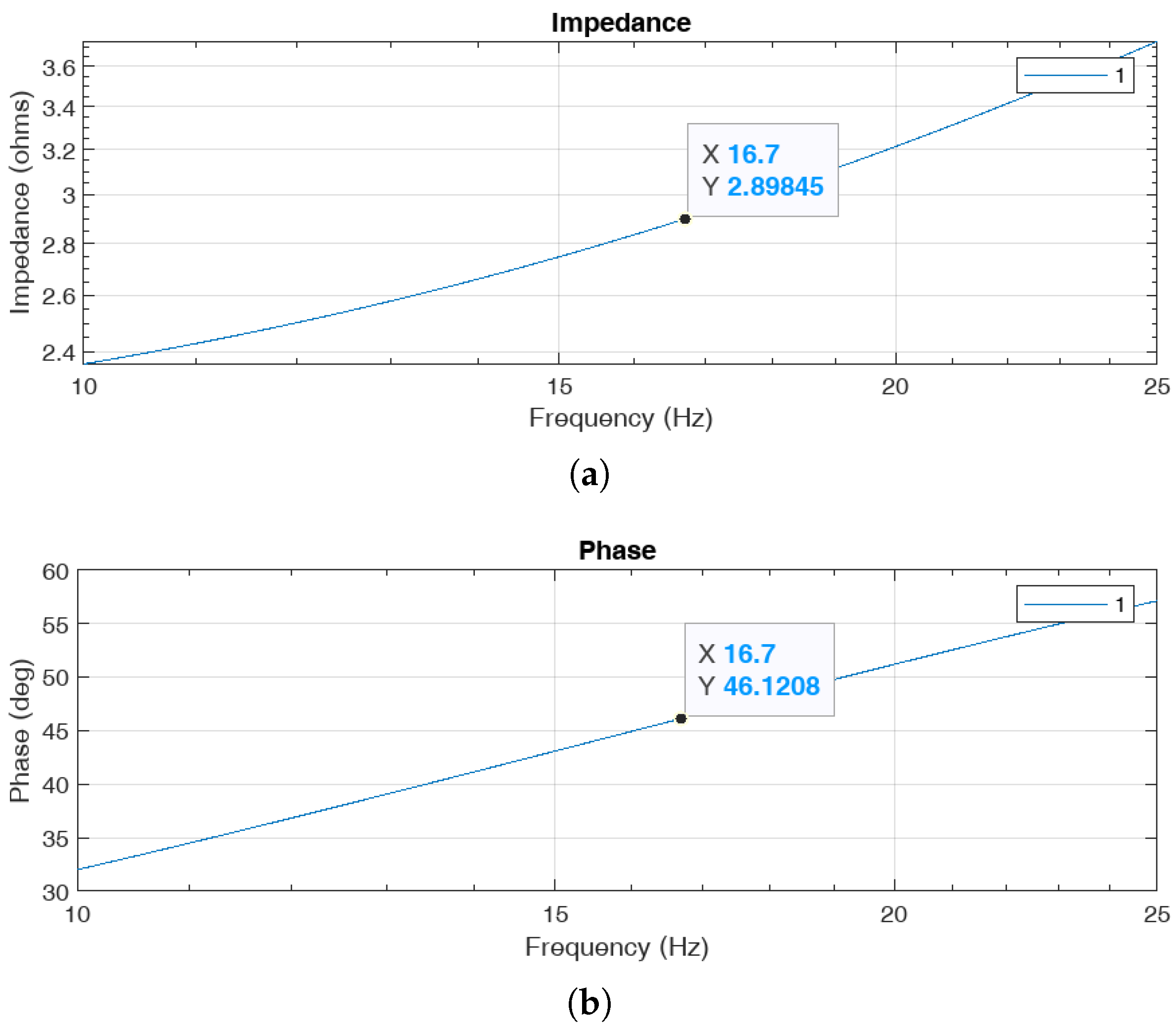
The network impedance was measured using the impedance tool of Matlab Simulink, which is insensitive to the distortion and power absorption variations. The result is shown in Figure 4. This value is used as reference ($Z_{n,1}^{\prime }$) when comparing the LMS and ACS algorithms.

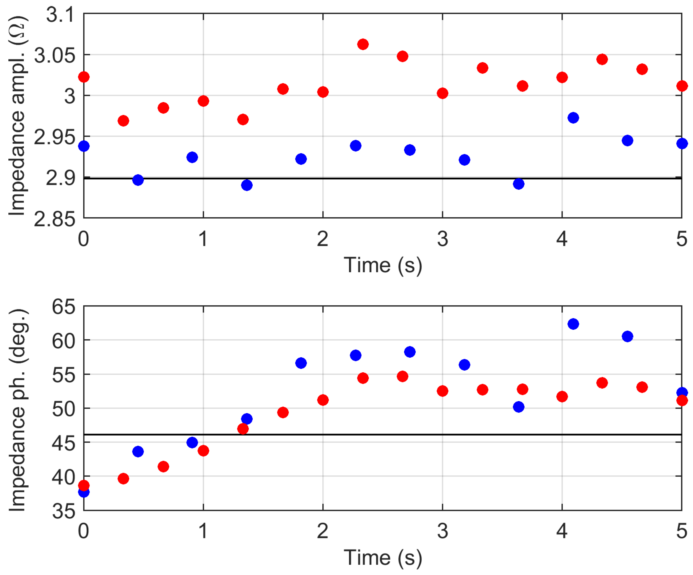
The LMS and ACS algorithms were run on the simulated waveforms after the extraction of the fundamental phasors over adjacent fundamental periods. The network frequency was fixed at $16.7$ Hz to avoid synchronization problems. The results are shown in Figure 5.

By observing the two sets of estimated ${\widehat{Z}}_{n,1}$ values in Figure 5 it is possible to conclude that both algorithms estimate the $Z_{n,1}^{\prime }$ reference impedance value correctly, with a better performance from the LMS algorithm, with less than 2% error on amplitude. The ACS algorithm in general slightly overestimates, with an error that may range up to about 5%. The behavior with respect to phase values is similar for both methods and, in general, the phase estimate is less accurate, although we know that amplitude accuracy is more relevant for the objectives of the present study.

After this positive preliminary check, the line impedance estimate was carried out with experimental data in the next section.

5. Results and Verification with Experimental Data

5.1. Description of the Measurement Setup and Collected Data

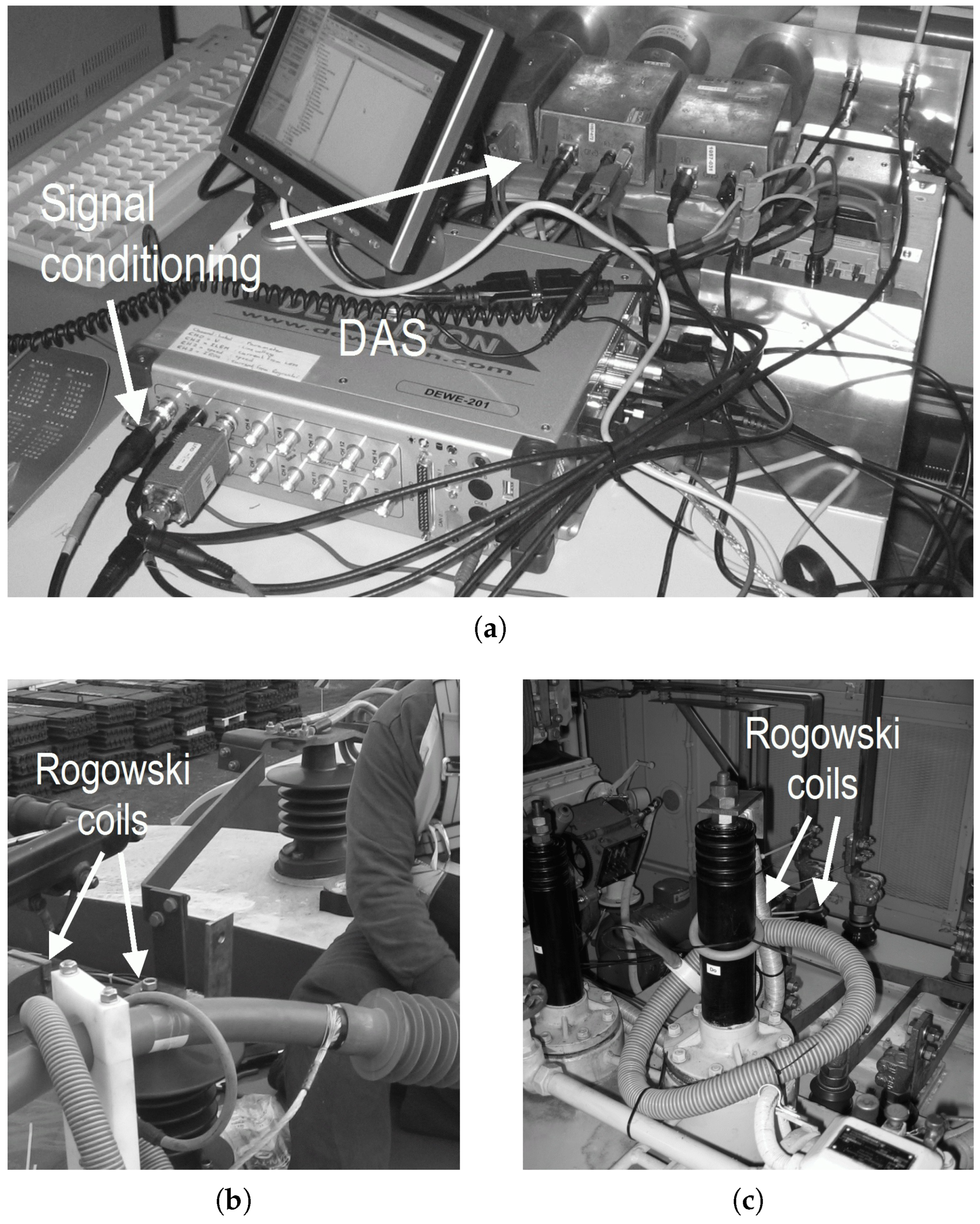
Data records measured along the Romanshorn–Zurich–Brig line of the 15 kV $16.7$ Hz Swiss network are used as the working example [33]. The characteristics of the measuring system were described in [59]: data acquisition (Dewetron, 16 bit), current probe (LEM Rogowski mod. 3010, gain 100 A/V), voltage probe (custom capacitive divider, gain 19,710 V/V calibrated for the Swiss installation). The measurement system is shown in Figure 6, using the material published in [59].

Sensitivity and uncertainty were estimated based on the internal noise sources and common error terms, such as eccentricity for the Rogowski coil and positioning error for the contactless capacitive sensor. The capacitive divider was calibrated on site after installation (ruling out major positioning errors) and the Rogowski was preliminarily calibrated at the laboratory (in addition to comparison with another Rogowski, also described in [59]). It was thus determined that the two measuring chains have a sensitivity of 1.2 mArms to 9 mArms for the 300 A to 3000 A scale setting and better than 4 Vrms, having a full scale in excess of 100 kV. The worst-case resulting uncertainty (at $k=1$) was determined as 3% and 1.5% for the current and voltage channels, respectively.

The uncertainty estimate was obtained including the following factors: positioning error, usually declared by manufacturers to be on the order of 1%; variability in response, as resulting from the standard deviation of collected repeated test results at different frequencies (type A uncertainty), taking care to cover the expected operating conditions in terms of dynamic range (e.g., changing fundamental current). The positioning error was then removed by on-site calibration after installation, keeping the sensors in a fixed position. For the Rogowski, slightly different frequency responses were observed depending on the amplitude of the bias current (i.e., $16.7$ Hz fundamental); excluding the results obtained in the laboratory at very low current intensity (less than 1 A), the residual dispersion for the entire excursion of the fundamental component was about 2.8%. The behavior of the voltage sensor, instead, was much more linear, resulting in an overall dispersion of about 1.1%.

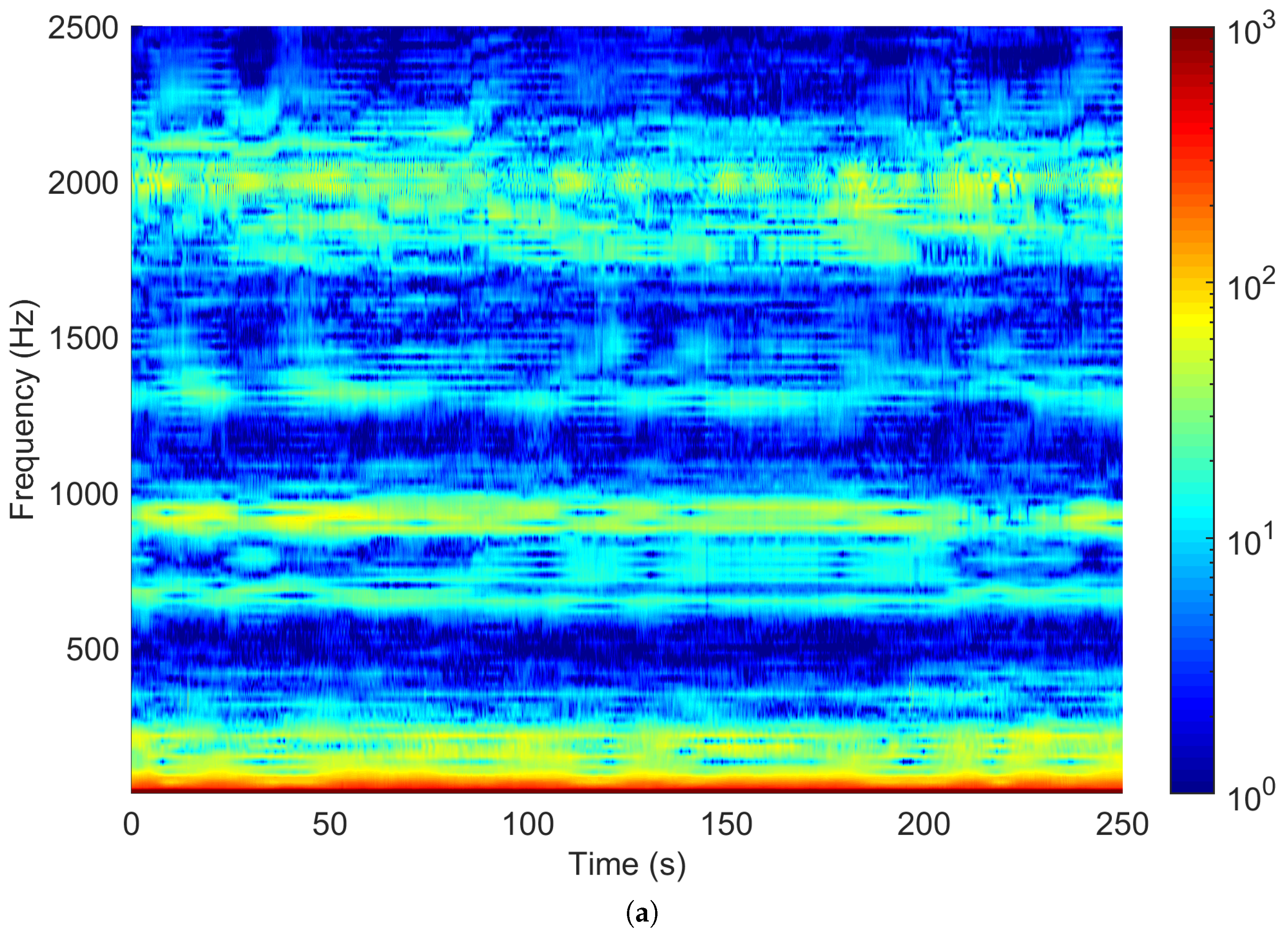
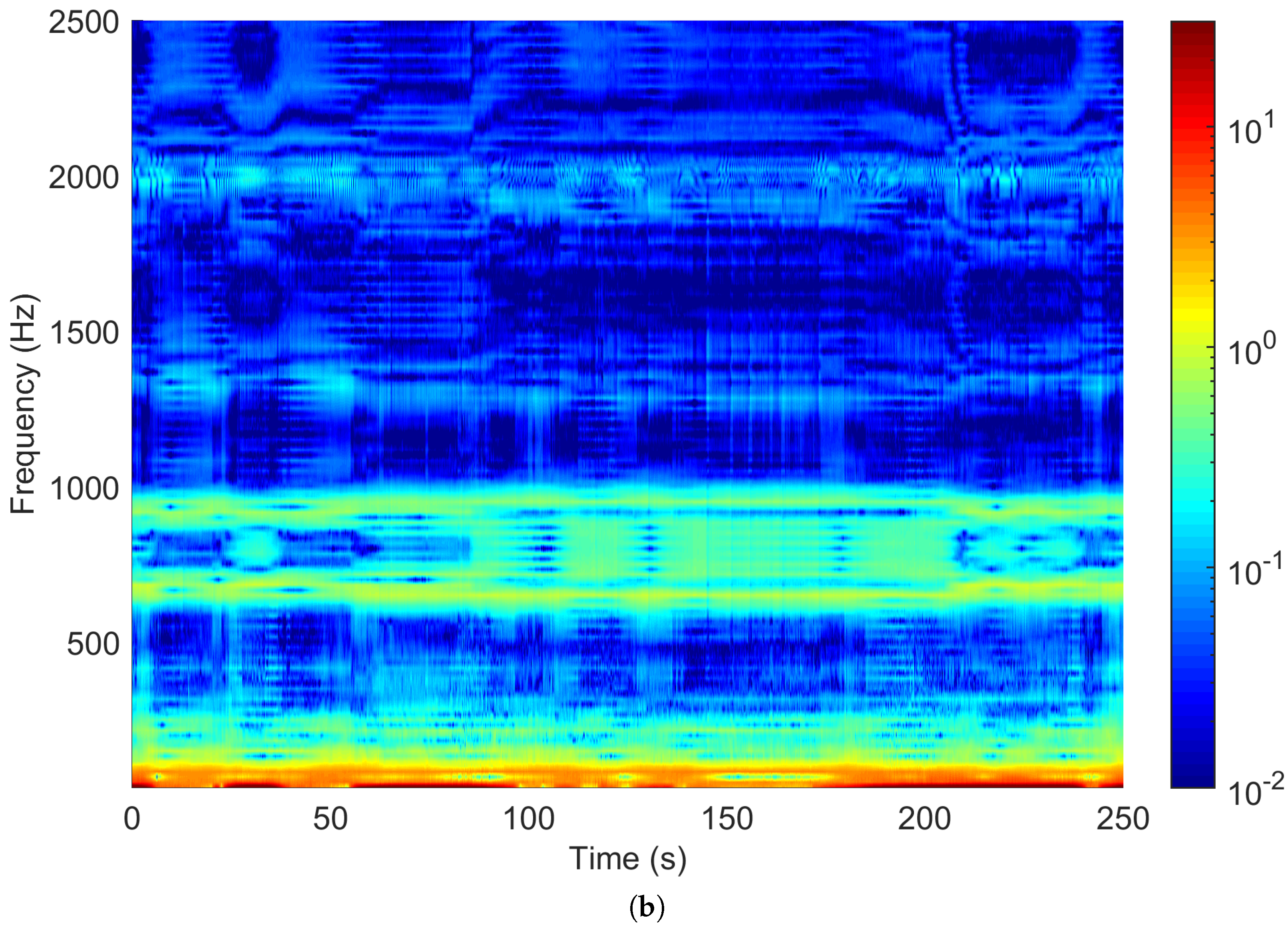
Since the analysis is limited to the fundamental, the harmonics represent a disturbance component: they are displayed in Figure 7 starting from the third harmonic for $V_p$ and $I_p$, over a short run of 250 s. The spectra $V_p\left(f\right)$ and $I_p\left(f\right)$ are shown in Figure 7 over the said run of 250 s having excluded the fundamental for a matter of dynamic range, to avoid compression of low-amplitude components. As for many railway lines, despite some regulatory constraints on current and voltage distortion, the distortion level in the recorded waveforms is quite high [28,30,60,61], thus representing a significant stress test for this type of algorithm.

Considering harmonics as disturbance, a method using phasor values calculated over a fundamental period T (or multiple), e.g., by means of Fourier analysis, is preferable to a method feeding instantaneous phasor values, such as a Kalman filter.

5.2. Details of Data Used for the Verification

Using the data introduced in Section 5.1, a long travel time of about 25 min is considered, where the train undergoes different supply conditions with different acceleration and deceleration profiles, in addition to stopping several times.

Such DFT phasors are thus calculated using a sliding window approach (short-time Fourier transform, STFT), and then, fed either to a quick static minimization method (the LMS), as per Section 3.1, or to the auto- and cross-spectrum calculation of Section 3.2. The two methods are applied iteratively over the train run to each $T_m$ interval with a sliding window approach.

The sliding window step is $s=p{T}_m$, with $0\le p\le 1$ being the overlap factor. With a fast execution of the LMS algorithm at each step s, real-time performance is achievable provided that acquisition and post-processing last for a shorter time than s (easily achievable with moderate calculation capability and s lying anywhere in the ms range).

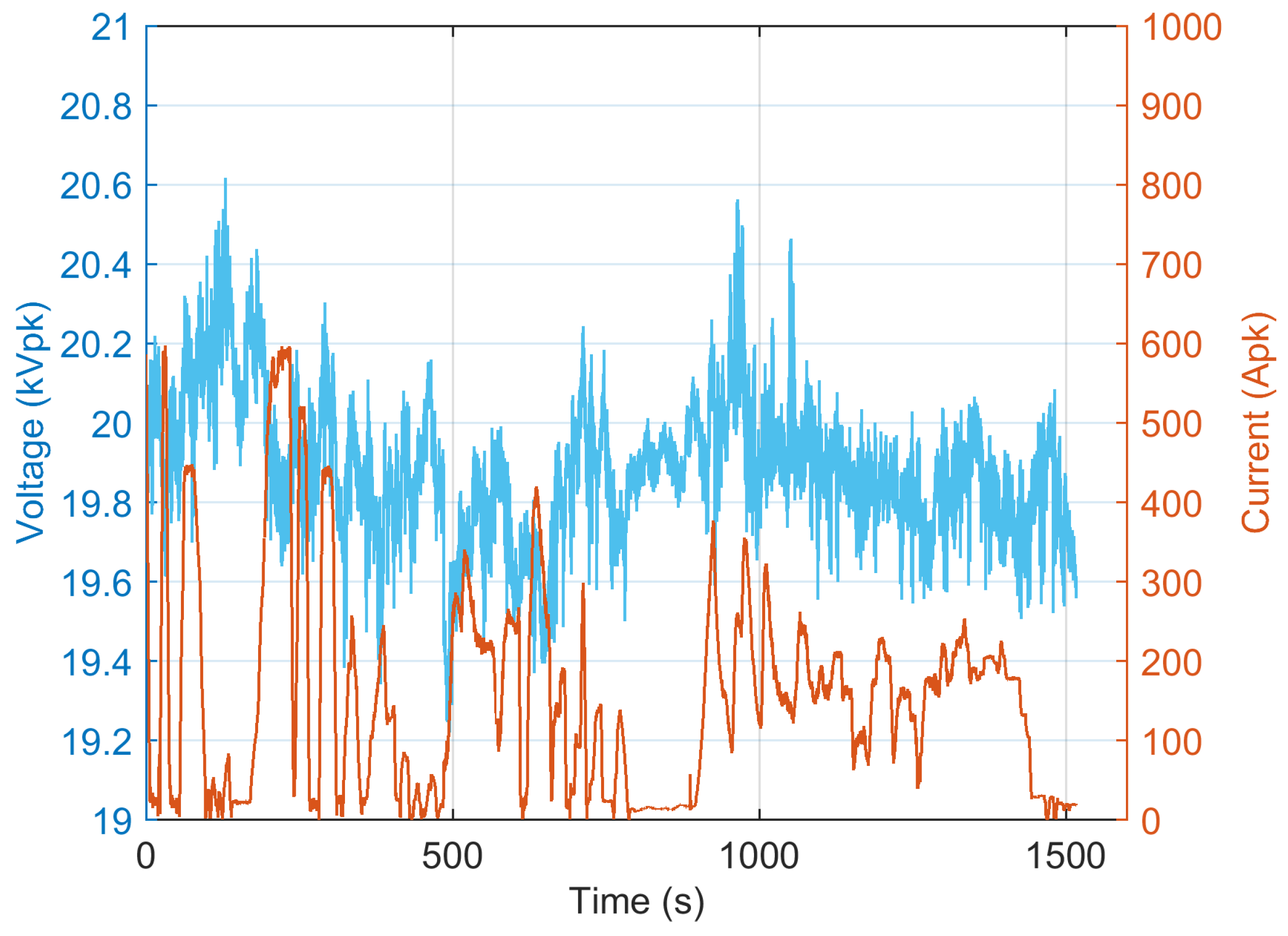
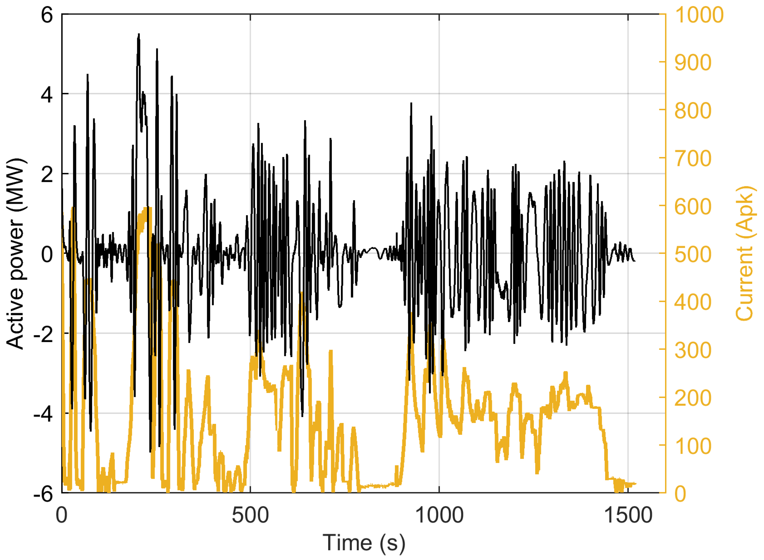
The overall peak values of the $V_p$ and $I_p$ fundamental components are shown in Figure 8, where the excursion of $V_p$ is 12% and the $I_p$ value (only the absolute value $|I_{p,1}|$ without a sign is shown in Figure 8) shows some intense and moderate acceleration and deceleration. The variability in the traction conditions can be observed better in Figure 9, where the active power at the fundamental $P_1$ is plotted with its sign, allowing for time intervals where the power flow reverses (regenerative braking) to be distinguished.

Whereas the intense accelerations are characterized by a unidirectional active power flow (e.g., between 4 and $5.5$ MW at about 250 s), at intermediate power levels the active power flow may be highly variable, alternating short intervals of traction to keep the speed to intervals of coasting or even slight braking to control the speed, for example, when approaching curves. As a consequence, the accuracy of the line impedance estimate is affected and such alternating behavior of the locomotive’s operating conditions represents a significant stress test.

Regarding the expected behavior of the line impedance at the fundamental, $Z_{n,1}$, being used as a benchmark, it must be underlined that the long line used for these measurements was not available for separate impedance measurements with a more traditional technique, such as an active method [62,63]. In addition, repeating the test for a sufficiently exhaustive number of locations to be representative over such a long line would be prohibitive in terms of time and cost.

The accuracy and reliability of the results is verified against known reference values for $16.7$ Hz systems, starting from the estimate of the TPS output impedance and of the per-unit-length line impedance.

AC railways operated at $16.7$ Hz have few isolating points (neutral sections) and in general TPSs may be connected in parallel (EN 50388-1 [64], Table 7), with an average separation distance of 30 km for non-high-speed lines ([64], Table H.1). Advisable values for the TPS power are on the order of 40 MVA to 60 MVA, from which at $V_n=15\mathrm{k}\mathrm{V}$ a base impedance is obtained in the range 3.75 $\Omega$ to 5.62 $\Omega$, and an assumption of a short-circuit ratio of about 5% leads to an equivalent TPS impedance $Z_{TPS}$ of 0.19 $\Omega$ to 0.28 $\Omega$ (purely inductive), to add then approximately 50 m$\Omega$ of transformer losses.

The impedance of the catenary system and return circuit may of course be accurately calculated once the arrangement of the line conductors is known, which is, however, variable between different locations. The advised value of $0.1+0.1i$$\Omega /\mathrm{km}$ of Table 9 in the EN 50641 [65] may be assumed as generally valid. The resistive part of the catenary system is prevalent compared to the resistive term of the TPS impedance due to transformer losses.

From this it is possible to determine a baseline for the estimated line impedance at a distance L in $\mathrm{km}$:

$${\widehat{Z}}_{n,1}=Z_{TPS}+L\times (0.1+j0.1)$$

(10)

The highest priority was given to testing the algorithm with experimental data that include realistic noise, small transients, variable operating conditions, and a complex set of power converters and loads onboard. The algorithm, in fact, relies on the solution for the equivalent circuit parameters $E_{n,1}$ and $Z_{n,1}$ of the network (left of “P” in the circuit of Figure 2) and the exclusion of the terms to the right of “P” of the circuit of Figure 2, and this is based on the assumption of what can be considered “steady” in the solution time interval $T_m$.

Other authors have instead provided more extensive results against simulated data, which are easier to collect and whose accuracy can be much better controlled, so that the accuracy of a new proposed method can be more thoroughly evaluated. Examples can be found in Arefifar et al. [52] and in Xia and Tang [66], with the latter proposing a very interesting technique based on Gaussian mixture regression applied to a range of harmonic frequencies. In this latter case, it is not clarified if the results comply with the expected physical behavior of a real network (as previously discussed at the end of Section 3), as the target harmonic impedance values were assigned somewhat arbitrarily; nevertheless, this technique is relevant and could be a natural extension of the present work.

5.3. Estimate of Line Impedance $Z_{n,1}$ at the Fundamental Using All Data

The first results are derived exploiting all the data and using an intermediate $T_m$ value with $M=12$, so a 720 ms interval, with a 300% sized sample vector compared to the minimum $M_{\min }=4$ previously identified. Interval times below 1 s, in fact, limit the uncertainty on the train position to less than its entire length even at high speed: at 250 km/h a train travels almost 70 m in 1 s, so that there is room enough for several seconds on conventional lines (limited usually to 160 km/h).

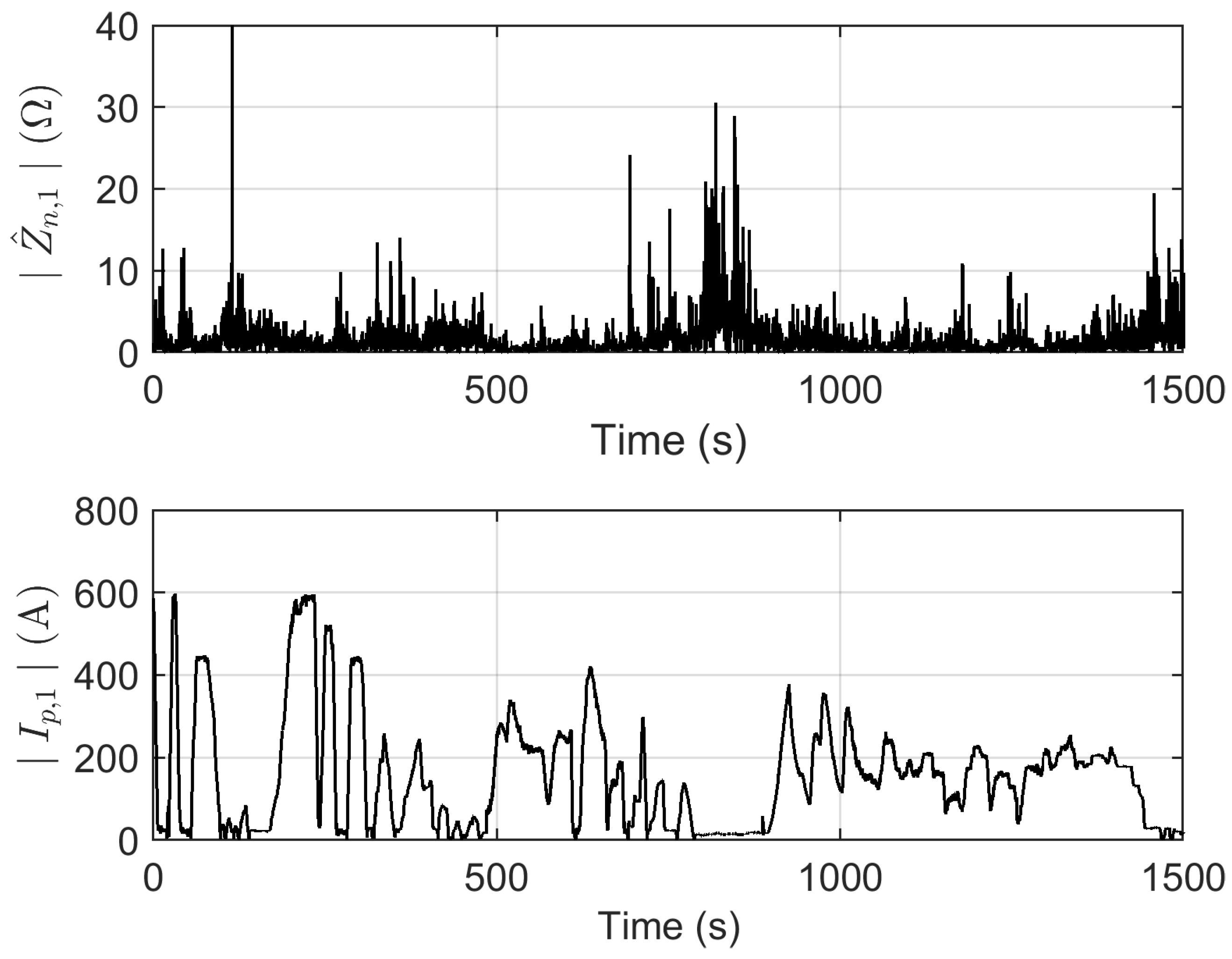
The results are shown in Figure 10, where the values of $Z_{n,1}$ are juxtaposed with those of the input current intensity $|I_{p,1}|$.

It is possible to see that the estimated $Z_{n,1}$ values are characterized by some bursts of points to quite large values; these are not due—as one may think—to resonances (we are at the fundamental frequency) or to a large distance from the TPS (such variation would be limited and always around values not causing an excessive voltage drop along the line itself, as one of the verified performance indexes for the power supply quality in railways). Such bursts are in reality caused by intervals where the current samples have a low value (as can be observed in Figure 10 by comparing the lower and upper insets). They correspond in general to the station stops when only the auxiliaries are operating rather than the traction converters, or to some coasting moments when no traction is applied.

The solution to this problem may be sought by feeding the algorithm with data vectors purged of low-amplitude current values, as discussed below in Section 5.4. It is briefly observed that this behavior is opposite to what is discussed in [14], where the grid voltage is instead estimated from the measurement of the voltage at the point of common coupling (the pantograph “P” in our case) in the time intervals at zero current. This feature is interesting and may be included in a more complex algorithm, which would, however, lose the simplicity and elegance of a pure LMS solution, as in the present case.

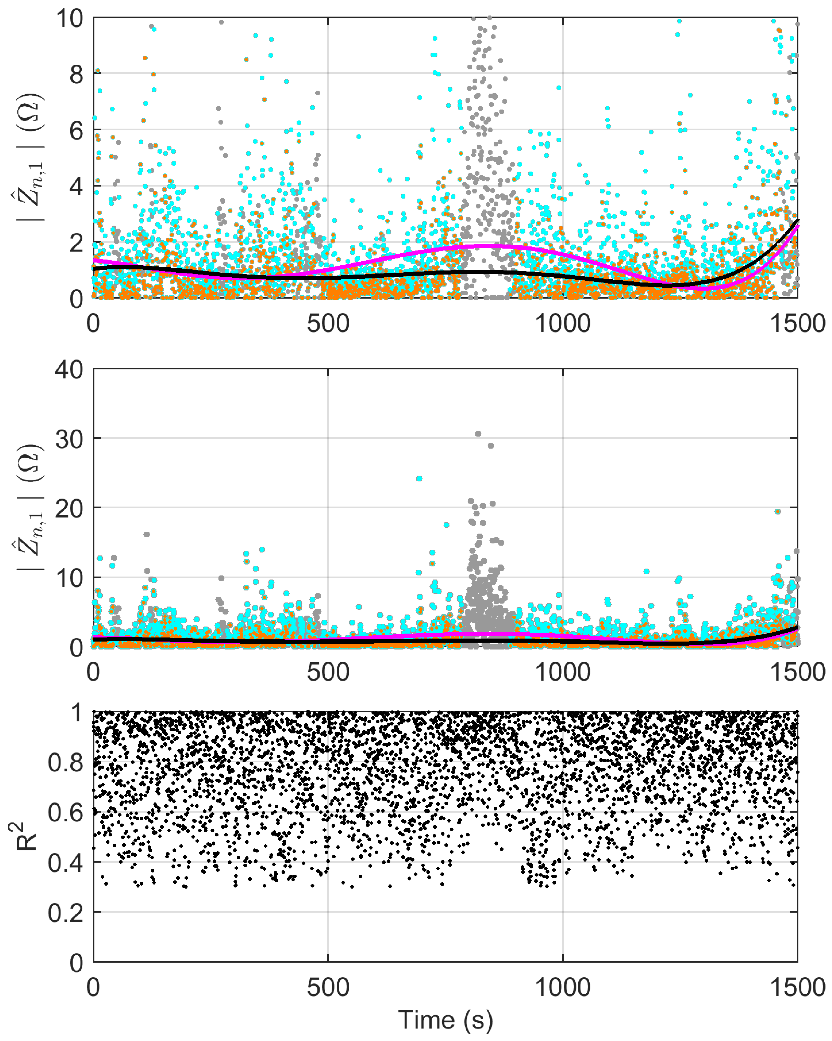
It is observed that large values of $R^2$ (one of the parameters for the goodness of fit) can be observed and they do not systematically correspond to low-current intervals, as is shown in the next section.

5.4. Line Impedance $Z_{n,1}$ Estimate Discarding Low-Current-Intensity Data

The simple rule of discarding samples featuring low intensity of the absorbed current is implemented with some different thresholds. If the long time intervals of station stops and of coasting are taken into account, this thresholding means dropping significant amounts of data: by selecting a threshold of 20 A (3.2% of the maximum absorbed current in Figure 8, 30% of data samples are discarded. This does not compromise the good and exhaustive estimate of $Z_{n,1}$ along the line, because most such data are related, as previously stated, to stops at stations; if the train does not change location, the equivalent line impedance $Z_{n,1}$ at its pantograph does not appreciably change (with a very minor contribution from the other running trains).

Goodness of fit is usually quantified by the mean squared error, MSE (the average of the squares of the residuals), or by the parameter $R^2$, that is the percentage of variance of $Z_{n,1}$ explained by the model-predicted ${\widehat{Z}}_{n,1}$. $R^2$ is selected in the following as representative of the error for its closer similarity to the magnitude squared coherence (MSC), that was introduced in Section 3.2 for the auto- and cross-spectrum (ACS) algorithm.

The result of using two criteria for the selection of the estimated points is shown in Figure 11, where three sets of ${\widehat{Z}}_{n,1}$ points are reported: gray points (set1) correspond to the original estimate using all points; light blue points (set2) are selected based on a current threshold (so discarding points with $Ip<I_{thr}$, with $I_{thr}=20 \mathrm{A}$); and orange points (set3) represent the further reduction of set2, adding the criterion that $R^2\ge R_{thr}^2$, with $R_{thr}^2=0.8$. Figure 11 also shows two interpolating lines obtained by fitting set2 and set3 points with an order five polynomial and drawn, respectively, in black and magenta. We can see that the two more or less correspond and that the improvement is mostly in the large burst of points in the middle of the run. A slight increase in the estimated impedance values may be seen at the end of the run.

5.5. Line Impedance $Z_{n,1}$ Estimate Using Auto- and Cross-Spectrum

In this section, the results of impedance estimation using the auto- and cross-spectra of $\Delta$ quantities, as discussed in Section 3.2, are reported. To support the discussion, the estimate obtained with the full quantities ($V_t$ and $I_t$) rather than the $\Delta$ quantities ($\Delta V_t$ and $\Delta I_t$) is also considered: it does not lead of course to the desired network impedance, but rather to an estimate of the input impedance of the rolling stock.

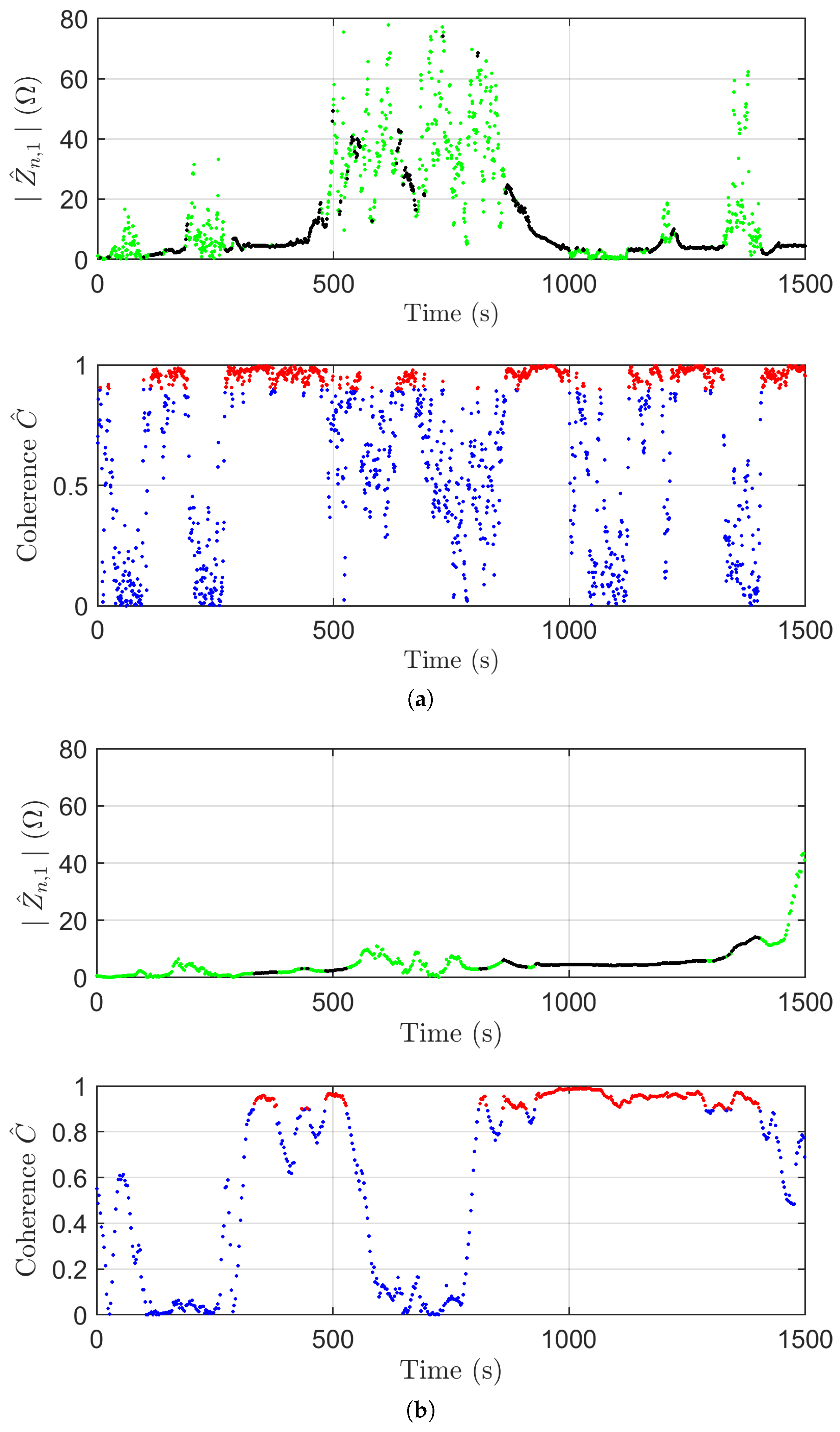
From Figure 12 it is possible to see that choosing $N_W=15$ marginally improves the quality of the Welch estimate of the spectrum (reducing the bursts of large-value points) and significantly reduces the clutter in both the estimate of $Z_{n,1}$ and related coherence values. At the same time, it is observed that the intervals with coherence above the chosen thresholds are reduced, because the larger the number of windows in the same Welch estimate, the higher the chance to find one or some of them significantly different from the adjacent ones.

There is also an apparent trend that biases the estimate, providing increasing values of impedance: although it must be underlined that both methods indicate a slight increase in the impedance towards the end of the run; the phenomenon is difficult to explain; it may be due to the fundamental frequency instability, that becomes more relevant the larger the interval of observation (that with the choice $N_W=15$ is three times larger). It must be noted that the estimate of coherence (that is the driving index to select the “good” intervals for the impedance estimate) is affected by any error in synchronization with a slightly varying system’s fundamental frequency: such errors would translate into a systematic error that is highly coherent.

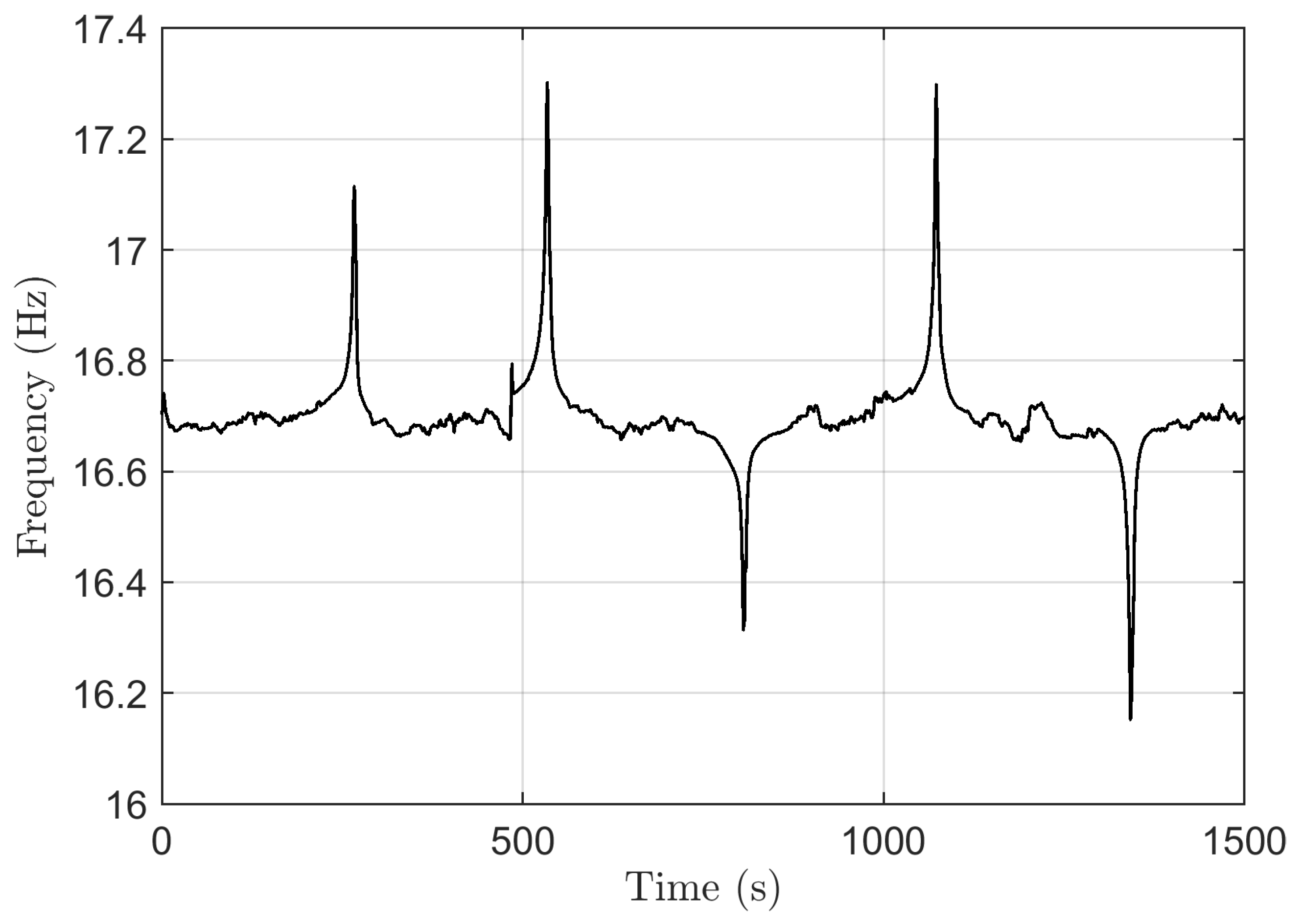
A snapshot of the instantaneous frequency estimated by FFT and parabolic interpolation is shown in Figure 13, where several impulse-like transients are visible (corresponding to the train stops): one at 500 s, where a step-like frequency change may be observed, caused by a change in power supply after a neutral section. This occurrence could have been identified in the previous Figure 10 by observing the small step-like instantaneous change in the $I_{p,1}$ current. The observed sudden frequency deviations are due to the worsening of the waveform quality at the train stops that causes larger errors in the estimate, not a real frequency deviation.

It may be concluded that the ACS algorithm is quite sensitive to frequency instability and the accuracy of the instantaneous frequency estimate; this is particularly evident in a railway system of the $16.7$ Hz type. On 50 Hz systems it has provided better results [51], as in Section 4 with synthetic data. An improvement would come from the wise selection and tuning of frequency estimate methods to the present case, as was discussed in [67]. Frequency instability and the difficulty of estimating it is surely a problem for islanded systems and distribution grids with highly distorted waveforms.

6. Conclusions

This work has briefly discussed the existing methods and applications of impedance estimation, considering first active and passive methods, and then, focusing on the latter from a single-point metering perspective. Presently, railway systems are not consistently and uniformly equipped with PMUs that allow exploitation of measurements at the two ends of a line section, including the moving points in the middle (i.e., the moving rolling stock).

The emerging need for energy accounting, however, makes the onboard metering equipment quite diffuse [31]. The proposed methods are based on the equations of the equivalent network impedance from a single-point perspective, i.e., seen from the rolling stock pantograph. Such equations are then solved by suitable techniques for over-determined systems, such as least mean squares (LMS), or exploiting auto- and cross-spectra of the difference voltage and current quantities (ACS method), in order to provide an estimate of the feeding line impedance.

The application to AC railway systems has been considered for load flow and power absorption optimization, focusing on the fundamental frequency and demonstrating the methods, with experimental results taken from the Swiss AC railway network [33].

The two LMS and ACS methods were first tested on a simulated synthetic network against a well-known reference impedance value and both provided an accurate estimate of the amplitude within 5%, with a slightly better behavior for the LMS method (the phase estimate is worse but for the present objective amplitude is more relevant).

With real data, the encountered problems are the stability of the fundamental frequency and its accurate estimate (considering the large distortion of the pantograph voltage and current waveforms), the presence of various types of transients, and, in general, noise and emissions from other trains and rolling stock items. Discarding data taken at low current intensity generally improves the estimate, avoiding the observed large spread of values especially at station stops when only onboard auxiliaries are operating with no traction. This, together with the selection of points with a large coefficient of determination $R^2$, makes the LMS estimate robust and preferable to that provided by the ACS method, that seems always too exposed to slight synchronization errors with respect to the instantaneous fundamental frequency.

The benefits of a sufficiently accurate estimate of the feeding line impedance seen by rolling stock leads to a better estimate of voltage drops and a better coordination of energy saving efforts, with better performance of the optimization algorithms.

Further potential developments and improvements could take three directions:

• A multi-frequency perspective, extending beyond the fundamental, including the most relevant harmonic components, considering the approach in [66];
• Exploiting calculations on adjacent frequency bins, which, by imposing the continuity and smooth behavior of the real system, improve the consistency of the estimate;
• Exploring alternative methods, such as the Gaussian mixture regression in [66], or improving the present methods, making the LMS and ACS part of a more complex estimation process that, for example, exploits intervals at low or zero current, as in [14], or improving the convergence using adaptive techniques, as in [68].

A method based on a Kalman filter [15] seems for the moment too exposed to the noise and variability in the system, having initially encountered difficulties in trimming its parameters for stability and accuracy when fed with real-world data. The objective is a flexible system that can be implemented in onboard energy meters with minimum complexity and computational effort.

The presentation and verification of these approaches were based on previous experimental results from railway measurements and were oriented to onboard implementation, mostly from the perspective of energy efficiency improvement, in particular with reference to the research carried out within the Project e-TRENY [69,70].

References

1. Boschetti, G.; Mariscotti, A. Integrated electromechanical simulation of traction systems: Relevant factors for the analysis and estimation of energy efficiency. In Proceedings of the 2012 Electrical Systems for Aircraft, Railway and Ship Propulsion, Bologna, Italy, 16–18 October 2012. [Google Scholar] [CrossRef]
2. Wang, K.; Hu, H.; Chen, J.; Zhu, J.; Zhong, X.; He, Z. System-Level Dynamic Energy Consumption Evaluation for High-Speed Railway. IEEE Trans. Transp. Electrif. 2019, 5, 745–757. [Google Scholar] [CrossRef]
3. Lin, J.; Song, J.; Lu, C. Synchrophasor Data Analytics: Transmission Line Parameters Online Estimation for Energy Management. IEEE Trans. Eng. Manag. 2022, 69, 671–681. [Google Scholar] [CrossRef]
4. Bhagat, S.; Bongiorno, J.; Mariscotti, A. Influence of Infrastructure and Operating Conditions on Energy Performance of DC Transit Systems. Energies 2023, 16, 3975. [Google Scholar] [CrossRef]
5. Huang, W.; Nengling, T.; Zheng, X.; Fan, C.; Yang, X.; Kirby, B.J. An Impedance Protection Scheme for Feeders of Active Distribution Networks. IEEE Trans. Power Deliv. 2014, 29, 1591–1602. [Google Scholar] [CrossRef]
6. Sivanagaraju, G.; Chakrabarti, S.; Srivastava, S.C. Uncertainty in Transmission Line Parameters: Estimation and Impact on Line Current Differential Protection. IEEE Trans. Instrum. Meas. 2014, 63, 1496–1504. [Google Scholar] [CrossRef]
7. Mariscotti, A. Impact of rail impedance intrinsic variability on railway system operation, EMC and safety. Int. J. Electr. Comput. Eng. (IJECE) 2021, 11, 17. [Google Scholar] [CrossRef]
8. Mariscotti, A.; Sandrolini, L. Detection of Harmonic Overvoltage and Resonance in AC Railways Using Measured Pantograph Electrical Quantities. Energies 2021, 14, 5645. [Google Scholar] [CrossRef]
9. Bhagat, S.; Mariscotti, A. Interference with Signaling Track Circuits Caused by Rolling Stock: Uncertainty and Variability on a Test Case. Electronics 2024, 13, 2875. [Google Scholar] [CrossRef]
10. Dommel, H.W. Overhead Line Parameters from Handbook Formulas and Computer Programs. IEEE Power Eng. Rev. 1985, PER-5, 38. [Google Scholar] [CrossRef]
11. Lucca, G. Per unit length parameters of a multiconductor line with earth return inside a tunnel. IEEE Trans. Electromagn. Compat. 2000, 42, 6–15. [Google Scholar] [CrossRef]
12. Deleanu, S.; Carpenter, D.C. A Study on Determination of Electrical Impedance and Frequency Characteristics of a Subway System Using Finite Element Analysis. In Proceedings of the 2013 Joint Rail Conference, Knoxville, TN, USA, 15–18 April 2013. JRC2013. [Google Scholar] [CrossRef]
13. Wu, M. Physical Interpretation of Impedance Formulas for Conductors Enclosed in a Cylindrical Tunnel. IEEE Trans. Power Deliv. 2011, 26, 1354–1360. [Google Scholar] [CrossRef]
14. Ciobotaru, M.; Agelidis, V.; Teodorescu, R. Line impedance estimation using model based identification technique. In Proceedings of the 2011 14th European Conference on Power Electronics and Applications, Birmingham, UK, 30 August–1 September 2011. [Google Scholar]
15. Hoffmann, N.; Fuchs, F.W. Minimal Invasive Equivalent Grid Impedance Estimation in Inductive—Resistive Power Networks Using Extended Kalman Filter. IEEE Trans. Power Electron. 2014, 29, 631–641. [Google Scholar] [CrossRef]
16. Borkowski, D. A new method for noninvasive measurement of grid harmonic impedance with data selection: Method for Noninvasive Measurement. Int. Trans. Electr. Energy Syst. 2015, 25, 3772–3791. [Google Scholar] [CrossRef]
17. Fernández, I.; Gallarreta, A.; González-Ramos, J.; Wright, P.; de la Vega, D.; Angulo, I.; Arrinda, A. Measurement System of the Mean and Sub-Cycle LV Grid Access Impedance From 20 kHz To 10 MHz. IEEE Trans. Power Deliv. 2023, 38, 2204–2212. [Google Scholar] [CrossRef]
18. Tang, J.; Xu, J.; Qian, J.; Chen, Z.; Yin, J.; Gao, Y.; Hu, Z. A precise measurement method for positive sequence parameters of EHV and UHV transmission lines and its application. In Proceedings of the 2011 IEEE Power Engineering and Automation Conference, Wuhan, China, 8–9 September 2011. [Google Scholar] [CrossRef]
19. Kurokawa, S.; Asti, G.A.; Costa, E.C.M.; Pissolato, J. Simplified procedure to estimate the resistance parameters of transmission lines. Electr. Eng. 2012, 95, 221–227. [Google Scholar] [CrossRef]
20. IEEE Std. 1870; IEEE Approved Draft Guide for the Parameter Measurement of AC Transmission Line. IEEE: Piscataway, NJ, USA, 2019.
21. Cecchi, V.; Leger, A.S.; Miu, K.; Nwankpa, C.O. Incorporating Temperature Variations Into Transmission-Line Models. IEEE Trans. Power Deliv. 2011, 26, 2189–2196. [Google Scholar] [CrossRef]
22. Naranpanawe, L.; Ma, H.; Saha, T. Overhead Conductor Condition Monitoring. 2018. Available online: https://www.energynetworks.com.au/news/conductor-condition-monitoring-milestone-1-report/ (accessed on 16 June 2024).
23. Afia, R.S.A.; Mustafa, E.; Tamus, Z.A. Aging Mechanisms and Non-Destructive Aging Indicators of XLPE/CSPE Unshielded LV Nuclear Power Cables Subjected to Simultaneous Radiation-Mechanical Aging. Polymers 2021, 13, 3033. [Google Scholar] [CrossRef]
24. Yang, J.; Li, W.; Chen, T.; Xu, W.; Wu, M. Online estimation and application of power grid impedance matrices based on synchronised phasor measurements. IET Gener. Transm. Distrib. 2010, 4, 1052. [Google Scholar] [CrossRef]
25. Asprou, M.; Kyriakides, E.; Albu, M.M. Uncertainty Bounds of Transmission Line Parameters Estimated From Synchronized Measurements. IEEE Trans. Instrum. Meas. 2019, 68, 2808–2818. [Google Scholar] [CrossRef]
26. Ćwil, M.; Bartnik, W.; Jarzębowski, S. Railway Vehicle Energy Efficiency as a Key Factor in Creating Sustainable Transportation Systems. Energies 2021, 14, 5211. [Google Scholar] [CrossRef]
27. Alonso, L.M.; Roux, L.D.; Taunay, L.; Watare, A.; Saudemont, C.; Robyns, B. Energy Metering Data Estimation and Validation in Railways. IEEE Trans. Power Deliv. 2022, 37, 4326–4334. [Google Scholar] [CrossRef]
28. Mariscotti, A. Results on the Power Quality of French and Italian 2 × 25 kV 50 Hz railways. In Proceedings of the 2012 IEEE International Instrumentation and Measurement Technology Conference Proceedings, Graz, Austria, 13–16 May 2012; IEEE: Piscataway, NJ, USA, 2012. [Google Scholar] [CrossRef]
29. Gao, S.; Li, X.; Ma, X.; Hu, H.; He, Z.; Yang, J. Measurement-Based Compartmental Modeling of Harmonic Sources in Traction Power-Supply System. IEEE Trans. Power Deliv. 2017, 32, 900–909. [Google Scholar] [CrossRef]
30. Kaleybar, H.J.; Brenna, M.; Foiadelli, F.; Fazel, S.S.; Zaninelli, D. Power Quality Phenomena in Electric Railway Power Supply Systems: An Exhaustive Framework and Classification. Energies 2020, 13, 6662. [Google Scholar] [CrossRef]
31. EN 50463-2; Railway Applications—Energy Measurement on Board Trains. CENELEC: Brussels, Belgium, 2017.
32. Giordano, D.; Clarkson, P.; Gamacho, F.; van den Brom, H.; Donadio, L.; Fernandez-Cardador, A.; Spalvieri, C.; Gallo, D.; Istrate, D.; De Santiago Laporte, A.; et al. Accurate Measurements of Energy, Efficiency and Power Quality in the Electric Railway System. In Proceedings of the 2018 Conference on Precision Electromagnetic Measurements (CPEM 2018), Paris, France, 8–13 July 2018. [Google Scholar] [CrossRef]
33. Mariscotti, A. Data sets of measured pantograph voltage and current of European AC railways. Data Brief 2020, 30, 105477. [Google Scholar] [CrossRef]
34. Monteiro, H.L.; Duque, C.A.; Silva, L.R.; Meyer, J.; Stiegler, R.; Testa, A.; Ribeiro, P.F. Harmonic impedance measurement based on short time current injections. Electr. Power Syst. Res. 2017, 148, 108–116. [Google Scholar] [CrossRef]
35. Hu, H.; Pan, P.; Song, Y.; He, Z. A Novel Controlled Frequency Band Impedance Measurement Approach for Single-Phase Railway Traction Power System. IEEE Trans. Ind. Electron. 2020, 67, 244–253. [Google Scholar] [CrossRef]
36. Ritzmann, D.; Wright, P.S.; Holderbaum, W.; Potter, B. A Method for Accurate Transmission Line Impedance Parameter Estimation. IEEE Trans. Instrum. Meas. 2016, 65, 2204–2213. [Google Scholar] [CrossRef]
37. Costa, E.C.M.; Kurokawa, S. Estimation of transmission line parameters using multiple methods. IET Gener. Transm. Distrib. 2015, 9, 2617–2624. [Google Scholar] [CrossRef]
38. Lin, Y.; Abur, A. A New Framework for Detection and Identification of Network Parameter Errors. IEEE Trans. Smart Grid 2018, 9, 1698–1706. [Google Scholar] [CrossRef]
39. Kodaira, D.; Park, J.; Kim, S.; Han, S.; Han, S. Impedance Estimation with an Enhanced Particle Swarm Optimization for Low-Voltage Distribution Networks. Energies 2019, 12, 1167. [Google Scholar] [CrossRef]
40. Song, K.; Mingli, W.; Yang, S.; Liu, Q.; Agelidis, V.G.; Konstantinou, G. High-Order Harmonic Resonances in Traction Power Supplies: A Review Based on Railway Operational Data, Measurements, and Experience. IEEE Trans. Power Electron. 2020, 35, 2501–2518. [Google Scholar] [CrossRef]
41. Ferrari, P.; Mariscotti, A.; Pozzobon, P. Reference curves of the pantograph impedance in DC railway systems. In Proceedings of the IEEE International Symposium on Circuits and Systems, Geneva, Switzerland, 28–31 May 2000. [Google Scholar] [CrossRef]
42. Holtz, J.; Kelin, H.J. The propagation of harmonic currents generated by inverter-fed locomotives in the distributed overhead supply system. IEEE Trans. Power Electron. 1989, 4, 168–174. [Google Scholar] [CrossRef]
43. Mariscotti, A.; Giordano, D.; Femine, A.D.; Signorino, D. Filter Transients onboard DC Rolling Stock and Exploitation for the Estimate of the Line Impedance. In Proceedings of the IEEE International Instrumentation and Measurement Technology Conference (I2MTC), Dubrovnik, Croatia, 25–28 May 2020. [Google Scholar] [CrossRef]
44. Seferi, Y.; Blair, S.M.; Mester, C.; Stewart, B.G. A Novel Arc Detection Method for DC Railway Systems. Energies 2021, 14, 444. [Google Scholar] [CrossRef]
45. Zhai, Y.; Liu, Q.; Wu, M.; Li, J. Influence of the Power Source on the Impedance-Frequency Estimation of the 2 × 25 kV Electrified Railway. IEEE Access 2020, 8, 71685–71693. [Google Scholar] [CrossRef]
46. He, F.G.; Li, C.Y.; Zhang, H.Y.; Ai, L.; Hu, H.T. Parallel Harmonic Resonance Probability Identification of Traction Power Supply System Based on Measured Data. Dianwang Jishu/Power Syst. Technol. 2024, 48, 2084–2094. [Google Scholar] [CrossRef]
47. Laury, J. Stability of Low-Frequency AC Railways—Models and Transient Stability. 2019. Available online: https://www.diva-portal.org/smash/get/diva2:1270596/FULLTEXT01.pdf (accessed on 16 June 2024).
48. Cobreces, S.; Bueno, E.; Pizarro, D.; Rodriguez, F.; Huerta, F. Grid Impedance Monitoring System for Distributed Power Generation Electronic Interfaces. IEEE Trans. Instrum. Meas. 2009, 58, 3112–3121. [Google Scholar] [CrossRef]
49. Mariscotti, A. Impact of Harmonic Power Terms on the Energy Measurement in AC Railways. IEEE Trans. Instrum. Meas. 2020, 69, 6731–6738. [Google Scholar] [CrossRef]
50. Langella, R.; Testa, A. A New Method for Statistical Assessment of the System Harmonic Impedance and of the Background Voltage Distortion. In Proceedings of the 2006 International Conference on Probabilistic Methods Applied to Power Systems, Stockholm, Sweden, 11–15 June 2006. [Google Scholar] [CrossRef]
51. Borkowski, D. Power system impedance tracking using sliding, finite memory complex recursive least squares. In Proceedings of the Signal Processing: Algorithms, Architectures, Arrangements, and Applications (SPA), Poznan, Poland, 26–28 September 2013. [Google Scholar]
52. Arefifar, S.A.; Xu, W. Online Tracking of Power System Impedance Parameters and Field Experiences. IEEE Trans. Power Deliv. 2009, 24, 1781–1788. [Google Scholar] [CrossRef]
53. Bendat, J.S.; Piersol, A.G. Random Data: Analysis and Measurement Procedures, 4th ed.; John Wiley & Sons: Hoboken, NJ, USA, 2010. [Google Scholar]
54. Piret, H.; Granjon, P.; Cattin, V.; Guillet, N. Online Estimation of Electrical Impedance. In Proceedings of the 7th International Workshop on Impedance Spectroscopy (IWIS 2014), Chemnitz, Germany, 24–26 September 2014. [Google Scholar]
55. Welch, P. The use of fast Fourier transform for the estimation of power spectra: A method based on time averaging over short, modified periodograms. IEEE Trans. Audio Electroacoust. 1967, 15, 70–73. [Google Scholar] [CrossRef]
56. Pintelon, R.; Schukens, J. System Identification: A Frequency Domain Approach; Wiley: Hoboken, NJ, USA, 2012. [Google Scholar]
57. Borkowski, D.; Wetula, A.; Kowalski, J. Uncertainty estimation in noninvasive measurement of harmonic impedance—Laboratory studies. In Proceedings of the 2015 International School on Nonsinusoidal Currents and Compensation (ISNCC), Lagow, Poland, 15–18 June 2015. [Google Scholar] [CrossRef]
58. Bartlett, M.S. Smoothing Periodograms from Time-Series with Continuous Spectra. Nature 1948, 161, 686–687. [Google Scholar] [CrossRef]
59. Mariscotti, A. Direct Measurement of Power Quality Over Railway Networks with Results of a 16.7-Hz Network. IEEE Trans. Instrum. Meas. 2011, 60, 1604–1612. [Google Scholar] [CrossRef]
60. Salles, R.S.; de Oliveira, R.A.; Ronnberg, S.K.; Mariscotti, A. Analytics of Waveform Distortion Variations in Railway Pantograph Measurements by Deep Learning. IEEE Trans. Instrum. Meas. 2022, 71, 2516211. [Google Scholar] [CrossRef]
61. Salles, R.S.; Rönnberg, S.K. Review of Waveform Distortion Interactions Assessment in Railway Power Systems. Energies 2023, 16, 5411. [Google Scholar] [CrossRef]
62. Bahrani, B.; Rufer, A.; Aeberhard, M. Railway catenary parameters identification based on harmonic current injection. In Proceedings of the 2011 14th European Conference on Power Electronics and Applications, Birmingham, UK, 30 August–1 September 2011. [Google Scholar]
63. Pan, P.; Hu, H.; Yang, X.; Blaabjerg, F.; Wang, X.; He, Z. Impedance Measurement of Traction Network and Electric Train for Stability Analysis in High-Speed Railways. IEEE Trans. Power Electron. 2018, 33, 10086–10100. [Google Scholar] [CrossRef]
64. EN 50388-1; Railway Applications—Fixed Installationsand Rolling Stock—Technical Criteria for the Coordination between Electric Traction Power Supply Systems and Rolling Stock to Achieve Interoperability. CENELEC: Brussels, Belgium, 2022.
65. EN 50641; Railway Applications—Fixed Installations—Requirements for the Validation of Simulation Tools Used for the Design of Electric Traction Power Supply Systems. CENELEC: Brussels, Belgium, 2020.
66. Xia, Y.; Tang, W. Study on Harmonic Impedance Estimation Based on Gaussian Mixture Regression Using Railway Power Supply Loads. Energies 2022, 15, 6952. [Google Scholar] [CrossRef]
67. Borkowski, J.; Kania, D.; Mroczka, J. Comparison of sine-wave frequency estimation methods in respect of speed and accuracy for a few observed cycles distorted by noise and harmonics. Metrol. Meas. Syst. 2018, 25. [Google Scholar] [CrossRef]
68. Li, M.; Zhang, Y.; Hu, Z.; Zhang, Y.; Zhang, J. A Battery SOC Estimation Method Based on AFFRLS-EKF. Sensors 2021, 21, 5698. [Google Scholar] [CrossRef]
69. e-TRENY. Metrology Support for Enhanced Energy Efficiency in DC Transportation Systems. Available online: https://e-treny.eu (accessed on 16 June 2024).
70. Giordano, D.; Fernandez, J.Q.; Gallo, D.; Hällström, J.; Istrate, D.; Jordache, M.; Mariscotti, A.; Rietveld, G.; Rovira, J.; Venugopal, P.; et al. Metrology Support for Enhanced Energy Efficiency in DC Transportation Systems. In Proceedings of the Conference on Precision Electromagnetic Measurements, Denver, CO, USA, 8–12 July 2024. [Google Scholar]
Figure 1. Simplified schematic of (a) a  16.7  Hz railway traction supply (from [8]) and (b) hot and cold paths (from [9], with slight modifications).
Energies 17 03739 g001
Figure 2. Equivalent circuit for the supply network (black, left of P) and rolling stock (light blue, right of P). The pantograph P is the tapping point at which the impedance estimate is carried out.
Energies 17 03739 g002
Figure 3. Simulated circuit including a generator and a feeding line connected to a single-phase rectifier with random power absorption level: (a) network schematic and (b) voltage (blue) and current (orange) waveforms.
Energies 17 03739 g003
Figure 4. Network impedance measured with the impedance tool of Matlab Simulink: (a) amplitude and (b) phase at the fundamental frequency of  16.7  Hz.
Energies 17 03739 g004
Figure 5. Comparison of the estimated network impedance at  16.7  Hz for the LMS (blue) and ACS (red) algorithms, together with the reference impedance value as in Figure 4 (amplitude and phase).
Energies 17 03739 g005
Figure 6. Measurement system showing (a) the data acquisition system together with filters (top right), and the Rogowski coils used during the tests positioned (b) on the locomotive roof and (c) on the onboard transformer’s primary terminal. (Reprinted with permission from IEEE Transactions on Instrumentation and Measurement [59]).
Energies 17 03739 g006
Figure 7. Overview of the pantograph spectra for (a) voltage  V p  and (b) current  I p  over a short run of 250 s (quantities at the fundamental are removed to increase the dynamic range of the vertical axis to improve the representation of the harmonic components).
Energies 17 03739 g007aEnergies 17 03739 g007b
Figure 8. Extracted fundamental component of  V p  and absolute value of  I p | I p , 1 | , vs. time.
Energies 17 03739 g008
Figure 9. Input active power compared to the absolute value of the  I p  fundamental  | I p , 1 |  vs. time.
Energies 17 03739 g009
Figure 10. ( Z ^ n , 1  vs. time by LMS algorithm including all samples (top), compared with the intensity of the input current at the fundamental  | I p , 1 |  (bottom).
Energies 17 03739 g010
Figure 11. Values of  Z ^ n , 1  vs. time showing a reduction in data dispersion and improvement in the estimate adopting two criteria on  I p , 1  amplitude and  R 2  amplitude: set1 with all data included (gray points), set2 with  I p < 20   A  (light blue points), and set3 with  R 2 0.8  (orange points). The two last sets lead to two interpolating curves of order 5, shown in black (set2) and magenta (set3).
Energies 17 03739 g011
Figure 12. Estimate of  Z n , 1  by the ACS algorithm for two different choices of the number of windows for the Welch spectra estimate: (a N W = 5 , (b N W = 15 . Intervals with coherence  C ^ ( t ) 0.8  are highlighted in red, and correspondingly, the estimate  Z ^ n , 1 ( t )  is plotted in black.
Energies 17 03739 g012
Figure 13. Estimate of the instantaneous fundamental frequency of the  16.7  Hz system using FFT followed by parabolic interpolation around the fundamental component.
Energies 17 03739 g013
Disclaimer/Publisher’s Note: The statements, opinions and data contained in all publications are solely those of the individual author(s) and contributor(s) and not of MDPI and/or the editor(s). MDPI and/or the editor(s) disclaim responsibility for any injury to people or property resulting from any ideas, methods, instructions or products referred to in the content.