Abstract
This study examined the price risk of the Belize–Mexico interconnection using ARMA-ARCH models to assess electricity pricing volatility and autoregression to determine the influence of conditional volatilities and import consumption. The findings revealed that the volatility of both markets, especially spot price, showed rare high-impact shocks and prolonged periods of volatile clusters. Volatile pricing tendencies, and forward pricing to a lesser extent, had positive effects on premiums. Premiums were largely dependent on pricing properties and system conditions of the supplier’s (Mexico) side, with negligible influence from the buyer’s (Belize) side. However, significant effects were found during certain hours with the buyer’s loading and transmission loss patterns. Practical implications revealed the possibility of occasional losses caused mostly by information delays and misalignment of risk factors and premiums, which could affect Belize’s power cost affordability and scheduling of local generation. Further research can broaden this current scope to enhance planning on local power supply by integrating current findings on the importation market behavior with the buyer’s local power expansion plan.
1. Introduction
Studies on energy security have emphasized implementation of strategies to achieve reliable and affordable quantities of energy supply under acceptable environmental consequences [1]. Strategies seek to diversify and weatherize the power supply mix, the collection of sources used to generate electricity [2], including locally installed power plants and supply chains of fuel imports. Less discussion was noted in the literature on cross-border trade, a centrally dispatched international electricity transmission system that directs energy from various stations to supply specific loads from a common power pool [3,4].
Oseni and Pollitt [5] found national electricity markets in advanced countries had evolved from (and for the purpose of supply to) local markets. Countries were reluctant to trade electricity across borders, but with limited resources and rising demand, jurisdictions like Bangladesh and India [6], Nepal [7], Switzerland [8], and regions across ASEAN [3] and North America [9] identified opportunities in cross-border trade as alternative sources of potentially cleaner and lower-priced electricity supply, alongside local generation. For example, Mexico reported a power capacity of 87,130 MW [10] and operated in the North American network with the United States and Canada, under the provision of the USMCA (United States–Mexico–Canada Trade Agreement) [11,12], and in Central America with interconnectivity to Belize.
Small developing nations face additional challenges, which threaten affordable self-sufficiency, given the scale of their power systems. The smaller nations are limited in their range of technological choices and opportunities for energy resource exploration. For example, Belize, with approximately 172 MW installed power capacity [13], has been supplementing its domestic power supply with electricity imports from Mexico since the early 1990s, via a physical interconnection as presented in Figure 1.
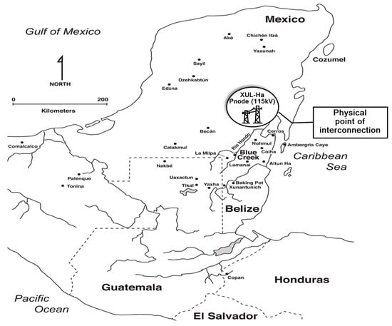
Figure 1.
This figure shows a regional map of northern Central America, including Mexico, adapted from Guderjan et al. [14], whereby the authors highlighted the 115 kV transmission line extending from point 1 (Xul-Ha, Yucatan Peninsula, Mexico) to point 2 (West Lake, Belize) that interconnects the power grids of both countries.
For Belize, like other small nations, cross-border electricity trade indirectly safeguarded the economy from external price shocks (unexpected shifts) on rising global energy commodity prices [15] but also exposed the local power market to price risks associated with procuring power from a foreign market. Belize’s local suppliers sold power on annualized fixed-cost pricing [16], but since Mexico liberalized its sector in 2013, electricity was sold under variable market-based pricing [17,18]. Belize imports averaged approximately 40% of the annual power supply, indicating significant price risks that could influence local supply investments and operational savings and spending due to deflationary and inflationary price volatility.
This Belize study expanded empirical research findings in the field of electricity contract pricing, including electricity forward and spot pricing, and market volatility [19,20]. This research also provided insights into the effects of cross-border electricity trade on small nations.
2. Background
2.1. Empirical Analysis of Electricity Forward and Spot Pricing
The efficient market hypothesis [21] in financial economics suggests that the commodity price incorporates all available market information and fosters trading at fair value in the absence of market inefficiency. However, empirical studies have identified information asymmetry in electricity prices [22], making some power markets less efficient. Consequently, it is important for small participants like Belize, who would be more exposed to asymmetric information, to understand the inefficiencies often embedded in pre-determined forward and spot pricing. Figure 2 presents a relationship of spot and forward pricing, highlighting how differences in expected pricing factors influence the level of basis risk.
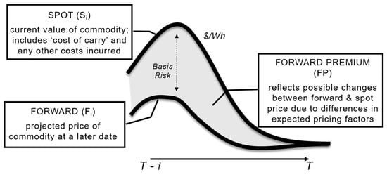
Figure 2.
This figure presents a representation of the time-dependent relationship between forward and spot pricing strategies and their influence on basis risk. Property of the authors.
Electricity is not directly storable (as electricity itself), so consumption and generation occur simultaneously [23]. Therefore, differences between forward and spot prices are strongly influenced by factors such as disruptions, congestion, demand surges, supply deficits, and with recent RE (renewable energy) integration, intermittent supply. Such characteristics result in the price of electricity exhibiting higher volatility and jumps than prices of conventional commodities [24].
Forward purchases allow buyers to mitigate adverse impacts of potential price increases. Forward premiums are the difference between spot and forward prices [19]. However, the effectiveness of this strategy for Belize depends on the country’s ability to anticipate precisely the amount of power required—because any excess is subject to real-time spot pricing, and shortfalls trigger penalties. Avoiding regular spot purchases is extremely challenging because of the number of factors stated earlier, which can result in differences between predetermined and real-time power supply and demand levels. Consequently, Belize’s deficit purchases also exhibit volatile tendencies and spikes over time. Similarly, forward contracts do not fully insulate Belize from risks associated with volatility and surges, which are inherent in forward pricing over time.
The discussed literature findings motivated this Belize study aiming to develop a methodological approach using time-series analyses. The current study investigated volatility and surges specific to electricity forward and spot pricing and assessed the effects on premiums favorable to Belize. Extant research has previously examined pricing time series of various markets in Mexico, where the National Electric System (SEN) comprises four subsystems. The largest subsystem, the National Interconnected System (SIN), covers 94% of federal entities. Seven control regions integrate SIN, with 101 load zones and 2356 nodes for electricity distribution [25], of which Belize’s power system interconnects at SIN’s ‘Xul-Ha’ node [16].
Rodriguez-Aguilar et al. [26] and De la Torre et al. [18] concentrated on developing modeling tools, including alpha-stable regressions and deep-learning models to generate price forecasts for Mexico’s wholesale power market. With a similar objective, Livas-García et al. [27] and Ramírez-García et al. [24] looked at the southeastern region of SIN and subsystems of SEN, respectively, but applied artificial intelligence (AI) approaches to generate price forecasts. These four past studies focused on obtaining highly accurate short-term predictions; however, this Belize study investigated the properties of the pricing series, including volatility and surges, to gain insight into the long-term behavior of the power market.
Quantitative analysis in this current study included two power systems, Belize and Mexico. However, using the Mexico system only, Rodriguez-Aguilar [26] identified qualitatively that congestion and loss were two components that determined the locational marginal price (LMP) of a SIN power node. Each component was based on the effect of increasing or reducing consumption on transmission line loadings, and the incidental line losses that accompanied the change. On the other hand, in this Belize study, patterns of consumption depended on electricity Belize imported, while the time-series analyses considered how technical conditions of the Xul-Ha Mexican node were influenced by Belize’s consumption and any statistically significant effect on the node’s LMPs.
2.2. Study Aim and Structure
The aim of this paper was to examine the dynamic exposure of Belize’s power system to the price risks associated with cross-border electricity trade. This study hypothesized that price risk exposure will be largely dependent on the pricing properties and system conditions of the supplier’s (Mexico) side with negligible influence from the buyer’s (Belize) side because of the huge difference in country size. This current research demonstrated the following relationships in the Xul-Ha node’s local marginal price: (i) an overall positive correlation with volatile tendencies of forward and spot pricing, (ii) the presence of premiums (if any) having a positive correlation with the volatile tendencies, and (iii) the presence of premiums (if any) having a statistically insignificant correlation with the loading and transmission loss patterns of the buyer’s (Belize) electricity import consumption.
Focusing on nodal data, analysis occurred for the trading node of the buyer, relying on information made public or accessible to foreign power purchasers. With derivative contracts increasing in popularity as financial risk management tools for electricity suppliers and as a potential discount medium for purchasers, this study incorporated forward premium, which received less attention in previous studies on Mexico’s power system. Furthermore, the analysis employed hourly measurements to improve our understanding of how pricing and nodal conditions varied during the day. Evaluating system conditions in the two nations simplified the assessment of the implications for Belize and Mexico’s intra-day trends on an hourly basis.
3. Materials and Methods
3.1. Study Design
The research design was composed of four stages, depicted in Figure 3, Figure 4, Figure 5 and Figure 6. Data were collected and summarized in Stage 1, using descriptive statistics that highlighted variability and distribution frequency in hourly electricity price per day, as shown in Figure 3.

Figure 3.
This figure depicts Stage 1 of the methodological approach consisting of data pre-processing and calculating summary statistics of hourly allocated forward and spot pricing.
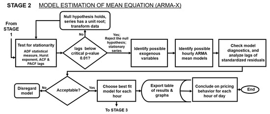
Figure 4.
This figure depicts Stage 2 of the methodological approach consisting of the development of ARMA-X models for changes in forward and spot pricing to construct mean models describing the autoregressive and moving-average trends of each pricing series per hour of the day.
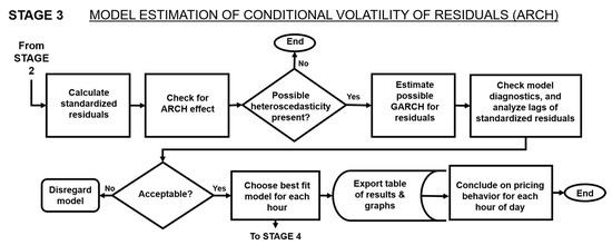
Figure 5.
This figure depicts Stage 3 of the methodological approach consisting of the development of ARCH models for the standardized residuals of ARMA-X models to construct conditional volatility series as risk measures describing the unexpected shifts of each pricing series per hour of the day.
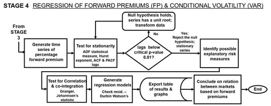
Figure 6.
This figure depicts Stage 4 of the methodological approach consisting of the development of VAR models to assess the influence on intra-day premiums by the risk measures of price, congestion, and generation represented by the unexpected shifts in each price series.
Model estimations (Stage 2), depicted in Figure 4, were used to draw generalized data-driven conclusions on each market’s characteristics and to develop a model for predicting electricity prices. This study applied a series of ARMAs (autoregressive moving averages) [28] for each hour of the day to construct an acceptable mean model of the historical price data, based on fundamental factors of electricity, with separate models for the forward and spot prices.
Price risks specific to the simulated ARMA-X electricity forward and spot pricing time series were captured in Stage 3 by modeling the conditional volatilities of the standardized residuals of each time series using ARCH (autoregressive conditional heteroscedastic) simulations [29], as depicted in Figure 5. A similar pairing of techniques was applied to analyze electricity price data in past work, including [30,31,32,33,34], and is detailed in Section 3.3.
Investigating the relationship between the forward premium and price risk factors associated with the Xul-Ha node using a series of hourly VAR (vector autoregression) models occurred in Stage 4 and is depicted in Figure 6. Assessment was performed on four risk factors, including the volatile tendencies and spikes specific to the forward and spot pricing, and variables reflecting potential effects on the nodal condition due to the buyer’s consumption activity.
3.2. The Data
The primary study data were hourly day-ahead forward and spot prices for electricity at the Xul-Ha node from 1 January 2018 to 31 December 2022. The dataset comprises the price for the day-ahead forward market where power delivery is made at the relevant hour the next day for each of the 43,824 intervals in the sample period. In each hourly period, the dataset included a spot price, allowing for real-time purchase. Also, the hourly electricity imported by Belize and Belize’s total electricity supplied to the grid were collected for the same study period. The price and power data were shared by Belize Electricity Limited (the buyer) after receiving a comprehensive description of the quantitative assessment for this research (data not publicly available).
Secondary research data were collected on daily weather conditions, natural gas price index, and electricity usage. Extant studies, such as [26], determined significant fluctuations in prices due to factors like seasonal demand, fuel availability, network congestion, and natural hazards. Similarly, another study [25] in Yucatan federal entity identified electricity generation (17.06%), fossil fuel costs (12.54% and 8.63%), load zone (11.17%), and day of the year (8.51%) as factors that affected locational marginal prices.
This Belize study retrieved daily average temperature data from the National Centers for Environmental Information [35] open-source portal for historical weather information from the Felipe Carrillo Puerto weather station and the Henry Hub Natural Gas Spot Index from the U.S. Energy Information Administration data portal [36]. Descriptive information, which served advisory purposes, on Mexico’s network structure was obtained from CENACE’s (the seller) market information system (SIM) public information on the wholesale electricity markets [37].
The collected data were analyzed for gaps and irregularities. The primary data, power pricing time series obtained directly from Belize’s electric utility, were deemed to be of good quality, with no gaps or abnormalities. A few gaps were discovered in the secondary data, specifically the web-based meteorological and natural gas index time series. Previous-day values were substituted into missing data fields to address the gaps.
3.3. Data Analysis
Data analyses for each stage of the methodological approach are undertaken as follows:
Stage 1:
This study generated the commonly applied measures, including mean, minimum, maximum, skew, and standard deviation. Rodriguez-Aguilar et al. [26] provided similar summary statistics for the wider SIN wholesale electricity market’s average LMP based on observations from January 2016 to 2017. Though the study period preceded this Belize study and was generated for the wholesale market, findings of both studies are comparable.
Stage 2:
The modeling estimations used daily changes in forward and spot price data, with an hour as the fundamental unit of analysis. This allowed for dampening extremities while maintaining data integrity.
An ARMA model [28] was used to fit an acceptable mean model that predicted average outcome value based on predictor variables, as defined in Equation (1).
where p is the autoregressive component, q is the moving average component, Xt and Xt−i are the values in the current period and previous i period, εt is the baseline constant, φi is the coefficient of the autoregressive (AR) component, θI is the coefficient of the moving average (MA) component, and εt−i is the error terms for the current period.
The data were divided into training and validation parts, 80% training and 20% validation. Before developing the model, changes in electricity prices were examined for stationarity using the Augmented Dickey–Fuller (ADF) test [38] to determine if there was a unit root, based on likelihood ratio statistics to reject the null hypothesis of non-stationarity in time series [39]. This study used autocorrelation and partial-autocorrelation functions (ACF and PACF) to assess the influence of lagged endogenous variables in the time series, using a correlogram to examine the ACF’s response to immediate impacts (the AR component) and PACF’s response to secondary impact (the MA component). The analysis incorporated exogenous factors of natural gas price index and average daily temperature, along with dummy variables for the month, day of the week, weekday, and weekend, as defined by the ARMA-X (with exogenous variable, X) [28] function in Equation (2).
where ηi is the coefficient of the exogenous input dt−i.
The time-series models, with and without exogenous factors, were optimized using the Auto Arima Python module [40], with values of p and q ranging from 1 to 10, based on minimization of the Akaike information criterion (AIC) using the Box–Jenkins approach [28]. The AR and MA components were deemed statistically significant with coefficients of p-values less than 0.05 and robust with total coefficients of less than one. The residuals’ ACF and PACF, and square of the residuals of the ARMA model residuals, were examined to confirm no autocorrelations, thereby suggesting the presence of the ARCH effect, deeming the mean model acceptable. In addition to the correlogram, the ARCH Lagrange Multiplier (LM) test [41] was applied to determine the presence of the heteroscedastic effect [29] of the residuals. The model estimation results were compared with real testing data using overall fit based on the lowest AIC.
Stage 3:
The ARMA estimates took into consideration autocorrelated aspects of power price, resulting in residuals associated with volatility. The volatility of these residuals was predicted using ARCH models, basic GARCH, and GJR-GARCH to account for possible asymmetry and leveraging, as specified in Equation (3).
where p is the order of GARCH term ϵt−i2; q is the order of ARCH term σt−i2; σ is unconditional variance; σt2 and σt−i2 are current and previous conditional variances, respectively; ϵt−i2 is the squared residual of the previous variance; αi is the coefficient for the previous squared residual; βi is the coefficient for the previous conditional variance; γi is the leverage parameter; and It−i is a dummy variable with the following stationary constraint:
Overall, four modeling combinations were used to determine volatility (GARCH and GJR-GARCH) and residual distribution (normal and skewed Student’s t, SST [42]). Model adequacy, overall fit, and accuracy were evaluated using information criteria (AIC), out-of-sample testing, and estimating the average and squared error, respectively. p-values were used to determine the importance of each model parameter. The coefficients of GARCH models were deemed statistically significant if they had p-values less than 0.05 and robust based on reviewing the ACF and PACF of their associated standardized residuals, which suggested that GARCH (1, 1) and GJR-GARCH (1, 1, 1) class models, where the order of p and q is 1, adequately captured the volatility in each hour.
Stage 4:
The final stage examined the relationship between electricity forward and spot prices, focusing on hourly time-varying forward premiums’ economic features and risk factors, estimating VARs using percentage forward premiums (FPit) as defined by Equation (4), where Fi,t−1 reflects the day-ahead forward price, and Sit reflects the day-of spot price for a daily interval, i, of a particular hour of day series.
The fundamental VAR assumption is that each variable, y, influences others within the hourly interval consisting of k time series, with the lagged values of all k time series serving as regressors [43]. As such, the VAR is defined in matrix form with a collection of endogenous variables, k, with p lags as follows:
where vector yt is the endogenous time series variables, c is the k-vector of constants, Φ is the time-invariant (k x k) matrix, and e is the k-vector of error terms.
The optimal lag, p, was determined by fitting increasing orders from 1 to 7, minimizing AIC, BIC, FPE, and HQIC [43]. In this stage, multiple information criteria were used due to the complexity of the multivariate VAR, reducing the likelihood of overfitting. The highest-performing lags were ranked and selected based on each criterion’s scoring. The VAR of the optimal order was fitted using Python’s StatsModels library, tsa (time-series analysis) module VAR [44]. The Durbin–Watson statistic [45] was calculated to detect residual patterns. These values ranged from 0 to 4, whereby a value close to 2 indicated no significant correlation, while values closer to 0 or 4 indicated positive or negative correlation, suggesting the need for model enhancements by altering the model’s order or predictor set, k.
The time series were tested for stationarity using the ADF test. The presence of causality and cointegration were assessed using Granger’s causality test [46] and Johansen’s statistic [47]. Granger’s causality test was used to examine the link between time series, with a p-value less than 0.05 indicating that a plausible correlation is present. Johansen’s test for cointegration was used to identify if the link between time series was statistically significant, determining if a linear combination of the series indicated a long-term significant link based on a 95% confidence interval.
In total, the study evaluated four risk variables. Following previous studies that performed similar empirical analyses on electricity prices, including [19,20,48] and past findings on Mexico’s SIN, our study determined that the pricing volatilities appropriately reflected real-time corrections of congestion, operating reserves, and transmission losses [26] by the supplier. Consequently, the time series of the simulated GARCH volatilities of the standardized residuals of spot and forward price changes, σ2S and σ2F, respectively, were chosen as the first two components to reflect the uncertainties associated with the supplier’s operations and system conditions at the Xul-Ha node.
Like any consumer, Belize’s consumption patterns affect the power flows and physical constraints at the delivery point interface. Further, the study considered that increasing and decreasing the output of local generation affects Belize’s transmission line loadings, incidentally varying the transmission line losses. Therefore, to determine the statistical significance of the buyer’s (Belize) relationship with the percentage forward premium, the analysis relied on two variables, namely (i) the hourly consumption of electricity imports, normalized between 0 and 1, delineated as IP, and (ii) the percentage difference between the normalized electricity imports and Belize’s total electricity supplied to the grid, D. The fundamental pricing elements of SIN’s LMPs suggest that both activities can affect congestion and incidental transmission loss components [26] at the Xul-Ha node, potentially impacting pricing. These variables represent variability in system conditions at the delivery node, which is fully concerned with the buyer’s activities.
4. Discussion of Results
4.1. Data Analysis of Forward and Spot Market Conditions
The time series plots for electricity imports forward and spot prices, allocated by hour of day, are presented in Figure 7. The data depicted alternating periods of volatility and calm, exhibiting a heteroskedastic effect, with rises in volatility particularly in late 2018, which coincided with the most recent reform revision restructuring of Mexico’s electricity sector [17].
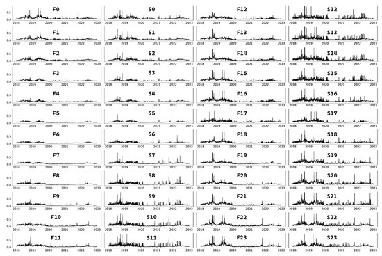
Figure 7.
This figure depicts the time series of day-ahead electricity forward prices (‘F’) and day-of electricity spot prices (‘S’) received by the buyer (Belize) from the Mexican export market at interconnection node, Xul-Ha, allocated by hour of day (‘0’ to ‘23’) for 2018 to 2022. Prices are expressed in US dollars per kilowatt hour.
Appendix A Table A1 reports the summary statistics for the electricity imports forward and spot prices. All prices are quoted in US dollars per kilowatt hour (USD/kWh). As shown, the average forward price fluctuated throughout the day, ranging from 0.057 USD/kWh in the 4th hour to 0.111 USD/kWh in the 21st hour. Overall, the lowest prices were observed in the early-morning hours, with average prices falling below the overall average of 0.083 USD/kWh from 0 to 9 h, gradually increasing throughout the remaining hours from the 10th to the 22nd hour, and then decreasing during the final hour of the day. Forward prices all returned positive skewness, indicating asymmetric tailing extending to more positive values for each hour’s distributions, with the most significant right-skewed tailing occurring during the afternoon-to-night-time hours, showing a high of 4.107 during the 18th hour. This finding was consistent with the right skewness reported in past studies of dynamic electricity pricing.
Based on standard deviations, forward prices, like other markets, displayed high intra-day variance. When the relative hourly ratios between the standard deviation and the mean value were compared, the highest variations occurred in the early afternoon from roughly the 12th to 15th hour and at night from the 20th to 22nd hour. For example, during the 15th hour, the standard deviation increased to almost 86% of its corresponding hourly mean value (0.096 USD/kWh) and was equal to the total mean for all hours of the forward prices (0.083 USD/kWh). The standard deviation exceeded this overall mean in the 20th and 21st hours. These results suggested that forward prices are particularly volatile during these hours.
Overall, forward price movements suggested an early-afternoon and night-time peak, consistent with extant findings [25] that linked the region’s climatic and geographical characteristics, as high temperatures prevail in the early afternoon, and demand for power increases once more during the last hours of the day for public, commercial, and residential lighting and air conditioning.
On an hourly basis, spot prices averaged around 0.015 USD/kWh higher than forward prices, resulting in a minimum of 0.07 USD/kWh in the 3rd and 4th hours, a maximum of 0.132 USD/kWh in the 21st hour, and an overall average of 0.098 USD/kWh. Overall, the average spot prices followed a similar hourly profile to average forward prices. Similarly to previously analyzed markets [19,34], spot prices showed higher overall right skewness than future prices; however, the maximum observed skewness of 4.088 in the 16th hour was less than the highest skew observed in forward prices.
The pattern of the magnitude of skewness also varied, occasionally appearing high in non-consecutive hours such as the 1st, 7th, and 13th hours, as opposed to future pricing, which showed larger skewness throughout successive afternoon and night-time hours. These findings demonstrated that contrary to the typical expectation, maximum forward prices may not be lower than maximum spot prices, particularly during odd hours such as the 14th, 15th, and 18th, with substantially right-skewed forward price distributions. This finding was not surprising as previous authors, including Ramírez-García et al. [24], emphasized that preconceptions on spot-to-forward relationships should be avoided by market participants, as electricity cannot be stored, and there is no specific formula for estimating the cost-of-carry difference between markets.
In contrast, the standard deviations of spot prices were uniformly greater than the equivalent standard deviations for forward prices, suggesting that spot prices are more volatile than forward prices and supporting the finding that, overall, spot prices are more right-skewed. However, analyzing the ratios of standard deviations and hourly means revealed that the variances fell more or less in line with those of the forward market, indicating that both markets are highly comparable in terms of volatility. The greatest variance was seen during the 21st hour, when the standard deviation (0.111 USD/kWh) matched the hourly mean while exceeding the overall mean by around 13%.
4.2. Time-Series Analysis for Determining Conditional Mean Equations for Pricing Series
In Appendix A, Table A2a,b contains the estimation results for the conditional mean equations on the change in electricity prices for day t to t − 1 using a system of autoregressive moving averages (ARMAs) based on information provided to the buyer for the forward and spot pricing, respectively.
For each hourly model, the sum of the autoregressive (AR) and moving average (MA) coefficients was less than one, suggesting that the ARMA process was stationary. Furthermore, the ACF and PACF of their standardized residuals revealed that no autocorrelated or partial autocorrelated lags (up to 30) exceeded the critical 5% level of significance. Additionally, all ARMA coefficients were statistically significant at the 1% level in each model. Notably, in addition to showing the validity of each equation for the conditional mean, these characteristics were also necessary for the subsequent volatility estimation of the residuals.
The study found that exogenous variables, average daily temperature, and the natural gas price index did not improve the mean models. The coefficient for average temperature was positive but statistically insignificant. Likewise, the natural gas energy index did not carry statistical significance on changes in forward pricing. For example, simulations showed the average daily temperature and gas price index had a directly proportional impact on the changes in forward prices, 1.17 × 10⁻⁵ and 5.77 × 10⁻⁵, respectively. However, both factors were insignificant (p-value = 0.56 and 0.88, respectively), and the base ARMA model resulted in a better overall fit in both cases (AICARMA = −7645.10 versus AICARMA-X = −7579.08). Therefore, estimating the electricity price change without the exogenous factors, when considering a full day’s profile, resulted in a better fit under the model selection criteria.
The insignificance of natural gas prices was in contradiction to Livas-García et al. [27] and Cruz May et al. [25], who previously determined that natural gas had the second-largest impact of 35.1% and 12.5%, respectively, on the value of the LMP using artificial intelligence and sensitivity analysis. This disparity may be due to the data analysis of this current study being conducted at the nodal level, unlike earlier studies that used regional estimates. The time difference between the reporting of the daily NG index and intra-day electricity pricing series must also be considered. With respect to the temperature indicator, average daily temperature might not have been as effective an indicator for the hour-by-hour analyses; however, due to data constraints, the study was limited to daily values.
Working versus non-workday variables were highly significant for a number of hours in both forward and spot markets. The weekend variable coefficient revealed both direct and inverse relationships in the forward and spot markets. Though highly statistical, these impacts were low in absolute terms, yet higher than the estimated impact of the workday dummy variable in the hourly models for which these variables were found to be significant.
Interestingly, the weekend variable’s coefficient did not consistently show a negative trend, contradicting the assumption that weekend prices are lower than weekday prices due to reduced congestion and reserves. Instead, individual hourly spot regressions showed a significant negative relation for 6 h and positive for 7 h, with the most significant negative relation occurring during the 0th hour, and the most significant positive relation occurring during the 21st hour.
Changes in forward prices reflected the information provided to the buyer on day t−1, hence, at the start of the buyer’s decision making process. The AR component suggested a directly proportional average impact of 0.40 on the price difference by its day-ago (lag 1) observation. Although highly statistically significant, this revealed a relatively low first-order correlation for a financial time series, but is consistent with extant findings and speaks to the volatile properties of the electricity commodity [30]. In turn, based on the MA component, the regressed residual of the day-ago observation revealed a significant inversely proportional average impact of 0.93 on changes in electricity price.
Spot prices reflected the information provided to the buyer on day t, hence, at a secondary stage of the buyer’s decision-making process. Its AR component suggested a considerably higher autocorrelation average impact of 0.79 compared to the changes in forward prices and for a financial time series for an electricity commodity when compared to previous market findings [22,30]. Similar to the changes in forward prices, the MA component of the day-ago observation revealed a significant inversely proportional average impact of 0.94 on the changes in spot prices.
4.3. Modeling the Volatility of Residuals as a Risk Measure for Pricing Series
In Appendix B, Table A3 presents the estimation results for conditional volatility models on the residuals of the change in forward and spot prices using an hourly system of generalized autoregressive conditional heteroskedastic (GARCH) models.
Reviewing the ACF and PACF of their associated standardized residuals suggested that GARCH (1, 1) and GJR-GARCH (1, 1, 1) class models adequately captured the volatility, and in all but one hourly model of forward residuals, the model fit and accuracy were improved by an assumed SST distribution of the residuals, as compared to a normal distribution.
The alpha and beta parameters were positive and highly statistically significant, suggesting that an increase in the lagged squared residuals (α) and lagged conditional variance (β) leads to an increase in the volatility. Moreover, the estimations observed that the beta effect was greater than that of the alpha for all hours of both the forward and spot changes in price residuals, suggesting that generally, there should be greater concern for the persistence of volatile periods versus the magnitudes of this volatility.
Figure 8 and Figure 9 provide depictions of sample hours of identical periods and comparative years for these simulations relative to the actual calculated volatility and stationary volatility. Stationary historical volatilities based on the value of standard deviation were estimated to measure the dispersion of daily fluctuations from 2018 to 2022 (a useful indicator for assessing risk over time and comparing it to dynamic volatilities generated by the estimated models).
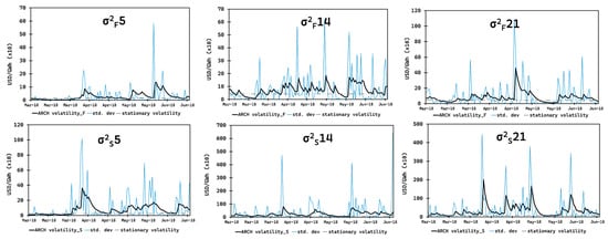
Figure 8.
This figure plots the simulated GARCH conditional volatility and standard deviations of daily changes in prices during certain hours from March to June of 2018 (corresponding to Belize’s dry season). The dashed line is the stationary volatility of the full dataset (from 2018 to 2022) for the given hour. From left to right, the first panel shows forward and spot prices for 5 a.m., the middle panel for forward and spot prices for 2 p.m., and the final panel for forward and spot prices for 9 p.m. Results are expressed in US dollars per kilowatt hour scaled by 104.

Figure 9.
This figure plots the simulated GARCH conditional volatility and standard deviations of daily changes in spot prices during the 2 p.m. hour from July to October (coinciding with Belize’s wet season) for different years. The dashed line is the stationary volatility of the full dataset (from 2018 to 2022) for the given hour. The top panel shows 2018, the middle panel is for 2020, and the bottom panel for 2022. Results are expressed in US dollars per kilowatt hour scaled by 104.
Visualizations of the ARCH-simulated volatilities showed presence of the clustering effect of price volatility. For example, following the simulated volatility line with the actual standard deviations, Figure 8 showed the simulated volatility increased across periods of high volatility and leveled-off during periods of low volatility. This contrast was observed more clearly during less volatile hours such as the 5 a.m. hour, and as shown in Figure 9, which reflects the same hour and period, but for differing years. Further, the visualizations demonstrated that reconstructed ARCH volatilities effectively captured the clustering effect, surpassing the use of information gathering based on stationary volatilities.
In cases where the GJR-GARCH outperformed the GARCH class, the gamma coefficients were all statistically significant and all negative for the forward price models but varied between positive and negative for the spot price models, suggesting a varied asymmetric response to positive and negative shocks across these hours. The negative relation of gamma in the forward price change models implied that positive changes in price (a daily electricity price increase) consistently caused larger variance, while the spot prices would experience the inverse effect for 11 of the 16 h where the asymmetrical effect proved significant.
The volatility of spot price changes was significantly higher than forward price changes, indicating greater long-term risk in the spot market. For hours from 7 to 16, and 20 to 21, spot volatilities were over 90% higher. Notably, an overlap was observed between these 12 h and the hours of gradual mean price increases in both markets, as per Appendix A, Table A1. Overall, the historical data revealed variations between the volatilities of forward and spot prices, in addition to their individual series’ intra-day variations, suggesting evidence of forward pricing compensating market participants for assuming risk. In this regard, risk premiums were present and primarily concentrated in the late-morning and late-night hours, averaging 12 h per day.
4.4. VAR Analysis for Determining the Presence of and Factors Influencing Premiums
The final set of results assessed the behavior of the relationship between electricity forward and spot prices, investigated by way of the percentage forward premiums (FPs). As depicted in Figure 10 and indicated in Appendix C, Table A4, similar to the average forward and spot prices, the average FP fluctuated throughout the day, ranging from a maximum of 51.3% during the 20th hour to a minimum of 7.3% during the midnight hour. The average FP and hourly skewness were all positive, large, and experienced significant variation across hours, as supported also by the changes in standard deviation. For example, on average, 19 of the 24 h showed an FP greater than 20%.
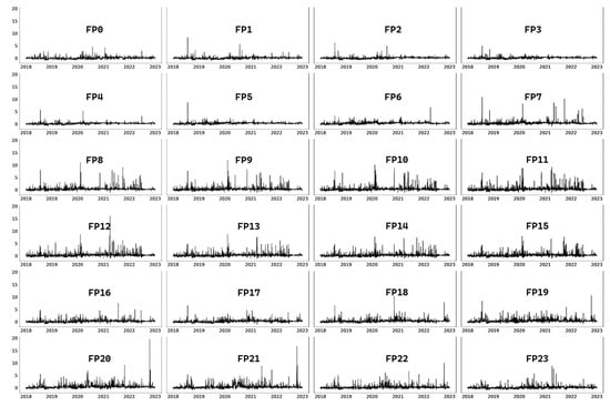
Figure 10.
This figure depicts the time series of the percentage forward premiums (‘FPs’) received by the buyer (Belize) from the Mexican export market at the interconnection node ‘Xul-Ha’ allocated by hour of day (‘0’ to ‘23’) from 2018 to 2022.
The magnitudes of the percentage premiums in this study may be most comparable to those seen in the German market [23,49] and the PJM market [22], while differences in datasets should be emphasized. Nonetheless, in this Belize study, positive risk premiums for certain hours were significantly larger than in other studies, suggesting that electricity markets are not yet fully settled into the restructured operating patterns following liberalization, especially for markets with short time frames like forward and spot, where pricing is observed within a day.
Additionally, unlike the other studies, this Belize study found negative premiums were not observed, even during off-peak hours, suggesting a persistent presence of risk factors like fuel availability and congestion at this particular node, and in turn, participants were highly risk-averse and rationally willing to pay significant premiums having understood these locational risk conditions. Premiums were not a focus of earlier research on the Mexican electricity market, making this element of the nodal findings difficult to relate to other nodes, or the regional or SIN level.
There were some peculiarities primarily concerned with a lack of the FP’s coincidence with unexpected shifts in the forward and spot markets. For example, the FP exhibited its first peak around the 8th hour and once more at the 20th hour, preceding the peak areas of the average forward and spot prices by approximately 2 to 3 h. Additionally, the skewness was found to be erratic, depicting sharp increases and decreases from hour to hour, unlike the heavy right-skewed tailing concentrated in the late-afternoon and night-time hours of the forward and spot electricity prices.
Seeing as the FP originated from a percentage of observations where the realized spot price is higher than the forward price, it was expected that the positive skewness of the forward and spot electricity data would drive the periods when the FPs were significantly impacted, as underlined by the models of [23,49]. However, the observed inefficiencies suggested timing concerns between the actual changes in the nodal system’s conditions and when their effects were reflected in the pricing series.
Further, these information time lags showed significant increases with volatility. Such findings implied that forward pricing does not move in steady correlation with the spot pricing. From Belize’s perspective, concerns can be raised over the adequacy of the hedging instrument that is applied in the forward market, whereby adequacy is indicative of the appropriateness of hedge timing and magnitudes, seeking to perfectly offset the forward-trade losses associated with its delivery node.
Our interpretations revealed that contrary to previous studies that investigated regional price averages, the highly locational aspect of the trade of electricity impacts the appropriateness of the applied hedging methodology and becomes more apparent in the analysis at the nodal level.
As the Xul-Ha node interfaces two independent power systems, its technical conditions are dependent on the patterns of generation, loading, and physical limitations of transmission as characterized by the operation and rated specifications of the two systems, but its hedging instrument may be largely reliant on the supplier’s side, as originally hypothesized.
For example, Belize’s power consumption data revealed high electricity import consumption between the hours of one and four, particularly during the dryer months of the year, in order to conserve water availability of the local hydropower plants during these very early morning, low-demand hours. In effect, the technical conditions of SIN’s Xul-Ha node may vastly vary compared to other local nodes that display standard intra-day patterns of loading.
With that key difference in mind, if Mexico’s regional operator applies a strategy in which localized hedging is relative to its larger geographic zone, such as the generation patterns and physical limitations of the node’s wider peninsula region, the disparity created by Xul-Ha’s unique loading pattern as a result of Belize’s consumption behavior creates the potential for a hedging practice that is, at times, excessive or too moderate.
As imperfect offsets (in magnitudes and timing) between forward and spot pricing at the node are observed, a plausible concern is the compatibility of the hedging methodology with the loading pattern’s physical limitations of a node that facilitates cross-border exchange and, in turn, identifies the factors on either sides of the interface that play the most influential roles in Xul-Ha’s local marginal pricing.
The VAR analyses explored this theory by modeling two sets of variables: pricing factor (conditional forward and spot volatilities) and nodal conditions (percentage power import, IP, and domestic generation factor, DF). The optimal FP VAR function for each hour is provided in Table 1, and matrices summarizing all variables are found in Appendix C, Figure A3. The analysis revealed significant links across variables, with premiums causally linked to forward and spot volatilities for all hours. Cointegration analysis revealed long-term, statistically significant relationships with both price factors. Full correlation and cointegration matrices are also available in Appendix C, Figure A1 and Figure A2.

Table 1.
1 This table provides a summary of the VAR analysis coefficients for the four factors (forward pricing volatility σ2F, spot pricing volatility σ2S, electricity import percentage IP, and percentage variation in local generation support D) assessed in relation to the percentage forward premium (FP) as presented in the function: .
The study found a direct relationship between premiums and unexpected shifts in spot pricing, but inversely linked to volatile forward pricing tendencies. The highest influence on the forward price (FP) was observed in hour 7 with 63%, suggesting that market participants may benefit most at this hour from forward purchases.
Further, based on the main cost components of spot pricing described by Rodriguez-Aguilar [26], this relationship can be linked to unexpected shifts in real-time system conditions, including deficiencies in operating reserves, congestion effects from increasing or decreasing supply resources or consumption, and the incidental effect on transmission losses. These corrections can be characterized by activities on both the supplier and buyer’s side, depending on the variables involved.
Consequently, we assessed nodal conditions from the perspective of the buyer’s load specifications and considered incremental energy transactions from the cross-border exchange (IP), as well as a variable measure of complementary generation from the buyer’s side (D). In turn, these relationships can lead to unexpected shifts in nodal conditions, influenced by congestion associated with consumption. These changes, unlike price factors, were primarily influenced by buyer activities, rather than price factors.
Our underlying theory suggested that price factors and supplier nodal conditions often overshadow buyer activity variation, leading to the assumption that Belize’s loading patterns, which were a variable of the Xul-Ha node’s power flows, will not significantly influence FP due to the significant size disparity between SIN and Belize’s power system.
However, the study found that Xul-Ha’s premiums decreased with higher electricity import consumption during certain hours, with the IP factor inversely correlated with FP. This effect was most significant during daytime hours 7–16 and night-time hours 19–20, with a maximum effect of 14% occurring during hours 12 and 16. Conversely, the nature of the relation between FP and D varied. For example, during the hours from 8 to 12, whereby D revealed plausible causality and long-term correlated significance, its impact on FP varied between positive and negative, suggesting that as Belize adds more local generation to complement power imports, premiums may reveal increases or decreases depending on the time of day. This activity, from the buyer’s side, is likely reflected in pricing through the varied nodal conditions of congestion and, incidentally, transmission losses. Still, both the impacts of IP and D, the resultant of the buyer’s activities, were significantly lower than the supplier’s, particularly the supplier’s activity as represented through the spot price factor.
An interesting aspect of the observed relationships were the high premium hours of 7 to 10 that were characterized by low demand on the supplier’s system, which coincided with highly volatile tendencies of spot pricing but low impact as a result of varying nodal conditions from the buyer’s side. Generally, the intra-day profiles assume higher system corrections during periods when the system is highly stressed [48]. However, this period neither aligned with the peak hours of SIN nor peak electricity imports from Belize’s system.
The volatile tendencies and high premiums during low-demand hours were likely due to supply resource and operating reserve corrections, which are entirely associated with the supplier’s system. According to Livas-García et al. [27] and Rodriguez-Aguilar et al. [26], SIN’s price volatility increases are generally caused by peak demand resulting from meteorological conditions, which causes high congestion [26], and to a lesser extent, increased power generation from renewable sources, which results in higher intermittent supply, particularly during peak conditions. In contrast to earlier studies, such as [22,49], more recent studies on FP have emphasized the uncertainties associated with capacity, particularly variable renewable energy (VRE) [34,48]. Viehmann [48] found that VRE, like wind power, shifts intra-day variations by supplying high production during low-demand hours, thereby linking economic risk to potential supply surplus and variability. Cruz May et al. [25] found that VRE has considerably influenced Mexico’s LMP price over time, and this behavior is linked to the recent start-up of wind power facilities in a number of load zones. As such, this VRE phenomenon presented a plausible source of the unexpected real-time shifts that resulted in relatively high FP during low-demand hours in this Belize study.
5. Conclusions and Practical Implications
This study proposed a methodological approach for understanding the associative effect of the cross-border supply on Belize’s price risk exposure. This methodology can be used by small market participants to conduct price analyses in liberalized electricity markets worldwide. Most crucially, the research design was based on the quality and timing of information received during the two major decision-making stages, allowing our findings to be readily integrated into the greater body of evidence on decision making and the costs associated with risk exposure of electricity imports compared to alternative power sources. This approach is reproducible for other participants and bidding zones, taking into account the differences in each zone (e.g., other nodes) and time intervals.
Data analysis highlighted that forward and spot pricing were lowest in early-morning hours, increasing gradually from the 10th to the 22nd hour and decreasing in the final hour. Price changes showed positive skewness, with the most significant right-skewed tailing occurring during afternoon-to-night-time hours. These behaviors proved consistent across both forward and spot pricing series; as such, from the perspective of an intra-day profile, we can first conclude that price risk exposure shows an overall positive association with expected price trend, which varies in magnitude across a given day.
Initially, we predicted a positive link between price risk exposure and the unexpected fluctuations in forward and spot pricing. Time-series analysis adequately captured autoregressive and moving-average trends, revealing unexpected shifts that may be analyzed using volatility models. Having established the latter, it was justifiable to proceed with the development of ARCH models to forecast and depict the conditional volatilities of the residuals of forward and spot price trends.
The market’s volatility revealed rare high-impact electricity price shocks, along with prolonged periods of volatile clusters, indicating that Belize’s reliance on this market mostly generated favorable economic returns, but occasional losses could potentially impact the affordability of local power costs, and the predicted association with price risk exposure was affirmed. Moreover, comparing the alpha and beta parameters, respectively, suggested that the duration of volatile clustering tends to be of greater concern than the size of the impact.
Evidence of hedging was determined. Estimates highlighted that Belize is compensated 7% to 51%, on average, via forward premiums for bearing intra-day risks, whereas trading in the spot market showed increased risk and procuring at higher price margins, which would likely magnify its economic losses. However, findings revealed the unexpected behavior observed across the changes in spot and forward prices does not transmit efficiently to the percentage forward premiums; thus, there are delays in the impact on these variables. Hence, in many instances, the Belize buyer could trade at a loss or not benefit economically because of mistiming when purchasing a substantial volume of electricity supply or, inversely, when purchasing a small quantity or not at all.
The study found that unexpected price shocks during morning hours had a greater impact on prices than the variation in nodal conditions due to electricity import consumption and local generation activities by the buyer. This suggested that real-time corrections on the supplier’s side have significantly greater influence on nodal conditions reflected in pricing than the buyer. The VARs noted periods with high FPs during low system demand and low import consumption that could be linked to uncertainties due to VRE’s introduced supply surplus and variability risks, thereby potentially impacting prior notions of premiums that primarily coincided with system peaks and high congestion. Still, contrary to the initial hypothesis, the buyer’s activities revealed a statistically significant effect associated with premiums during certain hours.
The practical implications of these findings revealed that both forward and spot prices can change rapidly and dramatically based on surprise news events, changes in supply and demand, and a host of other factors. However, the evidence identified that these risks were associated more highly with spot pricing. Purchasing electricity imports via the forward market provides the opportunity to profit from or hedge against price movements, particularly during hours where the percentage forward premiums are highest. Perfect foresight into markets is hindered by information lags, which were shown to misalign with heightened periods of risk factors and heightened periods of premiums. However, hedging does not necessarily imply buying electricity forward (like the case for power purchase agreements) but can be instituted as a purely financial instrument through contracts for difference or futures. These implications can influence future research that could further enhance planning and decision making on local power supply, for example, integrating the findings on the importation market behavior with the buyer’s local power expansion plan. Notably, the findings of this analysis are dependent on the provisions defined by the power purchase agreement of the Belize–Mexico interconnection during the period of this study (2018 to 2022). As a result, possible changes in the local or bi-lateral market situations can cause the results to differ. In turn, future work can address this limitation by conducting model-based studies in contrast to econometric analyses, whereby various market conditions can be defined and simulated through multiple scenarios.
Author Contributions
K.S.U.: conceptualization, methodology, formal analysis, data curation, writing—original draft preparation; B.C.M.: writing—review and editing, supervision. All authors have read and agreed to the published version of the manuscript.
Funding
This research received no external funding.
Data Availability Statement
The raw data are unavailable due to institutional privacy restrictions.
Acknowledgments
The authors gratefully acknowledge the local stakeholders of Belize, including Belize Electricity Limited, the Public Utilities Commission, and the Ministerial Energy Unit.
Conflicts of Interest
The authors declare no conflicts of interest.
Appendix A. Forward and Spot Pricing

Table A1.
This table provides summary statistics for the hourly forward and spot electricity prices received by the buyer (Belize) from the Mexican export market at the interconnection node ‘Xul-Ha’. The sample includes daily observations for each of the 24 h from 2018 to 2022. Prices are expressed in US dollars per kilowatt hour.
| Hour | Mean | Min. | Max. | Skew | Std. Deviation | |||||
|---|---|---|---|---|---|---|---|---|---|---|
| Forward | Spot | Forward | Spot | Forward | Spot | Forward | Spot | Forward | Spot | |
| 0 | 0.076 | 0.091 | 0.017 | 0.028 | 0.372 | 0.619 | 1.598 | 2.423 | 0.047 | 0.056 |
| 1 | 0.068 | 0.082 | 0.016 | 0.019 | 0.343 | 0.784 | 1.796 | 3.798 | 0.042 | 0.052 |
| 2 | 0.062 | 0.075 | 0.015 | 0.016 | 0.296 | 0.579 | 1.602 | 3.271 | 0.035 | 0.043 |
| 3 | 0.058 | 0.070 | 0.013 | 0.015 | 0.288 | 0.579 | 1.549 | 3.192 | 0.031 | 0.037 |
| 4 | 0.057 | 0.070 | 0.015 | 0.014 | 0.188 | 0.410 | 1.193 | 2.224 | 0.030 | 0.035 |
| 5 | 0.060 | 0.073 | 0.015 | 0.014 | 0.200 | 0.593 | 1.146 | 2.670 | 0.032 | 0.037 |
| 6 | 0.064 | 0.077 | 0.012 | 0.016 | 0.290 | 0.587 | 1.090 | 2.289 | 0.035 | 0.040 |
| 7 | 0.070 | 0.083 | 0.014 | 0.017 | 0.409 | 0.801 | 1.563 | 4.002 | 0.041 | 0.053 |
| 8 | 0.076 | 0.091 | 0.006 | 0.008 | 0.439 | 0.777 | 1.537 | 3.159 | 0.048 | 0.062 |
| 9 | 0.081 | 0.097 | 0.013 | 0.017 | 0.302 | 0.927 | 1.114 | 3.237 | 0.052 | 0.069 |
| 10 | 0.086 | 0.102 | 0.012 | 0.015 | 0.744 | 0.927 | 1.986 | 3.464 | 0.059 | 0.077 |
| 11 | 0.089 | 0.105 | 0.012 | 0.021 | 0.535 | 0.927 | 1.907 | 3.249 | 0.063 | 0.081 |
| 12 | 0.091 | 0.107 | 0.012 | 0.021 | 0.801 | 0.927 | 3.338 | 3.384 | 0.071 | 0.082 |
| 13 | 0.093 | 0.107 | 0.012 | 0.022 | 0.800 | 0.927 | 3.820 | 3.823 | 0.078 | 0.086 |
| 14 | 0.094 | 0.108 | 0.012 | 0.008 | 0.801 | 0.927 | 3.578 | 3.558 | 0.079 | 0.087 |
| 15 | 0.096 | 0.110 | 0.012 | 0.021 | 0.801 | 0.925 | 3.552 | 3.186 | 0.083 | 0.087 |
| 16 | 0.090 | 0.103 | 0.012 | 0.016 | 0.781 | 0.927 | 3.194 | 4.088 | 0.067 | 0.076 |
| 17 | 0.085 | 0.099 | 0.013 | 0.027 | 0.512 | 0.864 | 1.682 | 2.896 | 0.054 | 0.061 |
| 18 | 0.092 | 0.107 | 0.020 | 0.027 | 0.802 | 0.926 | 4.107 | 3.279 | 0.069 | 0.071 |
| 19 | 0.101 | 0.118 | 0.021 | 0.030 | 0.802 | 0.926 | 3.289 | 3.346 | 0.074 | 0.084 |
| 20 | 0.108 | 0.127 | 0.021 | 0.031 | 0.802 | 0.934 | 3.486 | 3.769 | 0.084 | 0.098 |
| 21 | 0.111 | 0.132 | 0.023 | 0.031 | 0.802 | 0.934 | 3.365 | 3.762 | 0.091 | 0.111 |
| 22 | 0.103 | 0.120 | 0.022 | 0.030 | 0.802 | 0.926 | 3.760 | 3.691 | 0.081 | 0.089 |
| 23 | 0.089 | 0.106 | 0.021 | 0.031 | 0.641 | 0.926 | 2.097 | 3.081 | 0.060 | 0.074 |

Table A2.
These tables contain the parameter values for the conditional mean equations of the change in electricity forward (a) and spot (b) prices using an hourly system of ARMA models with selection criteria based on prediction error and quality of fit (Akaike information criterion, ‘AIC’), out-of-sample testing (mean square error, ‘MSE’), and parameter significance using the critical p-value (1% ‘very significant’, as indicated by (**) and 5% ‘significant’, as indicated by (*)). (~) Coefficient result provided ‘if applicable’ to the selected model.
| (a) Forward Pricing | |||||||
|---|---|---|---|---|---|---|---|
| Hour | AR | MA | Dummy Variables | ||||
| Lag 1 | Lag 2 | Lag 3 | Lag 1 | Lag 2 | D_weekend | D_weekday | |
| 0 | 0.229 ** | −0.825 ** | −0.005 ** | 0.002 ** | |||
| 1 | 0.342 ** | −0.867 ** | −0.005 ** | 0.002 ** | |||
| 2 | 0.386 ** | −0.895 ** | |||||
| 3 | 0.372 ** | −0.869 ** | −0.003 ** | 0.001 | |||
| 4 | 0.372 ** | −0.869 ** | −0.003 ** | 0.001 | |||
| 5 | 0.287 ** | −0.829 ** | −0.004 ** | 0.002 | |||
| 6 | 0.363 ** | −0.862 ** | −0.003 ** | 0.001 | |||
| 7 | 0.405 ** | −0.895 ** | −0.002 ** | 7 × 10⁻⁴ * | |||
| 8 | 0.362 ** | −0.920 ** | |||||
| 9 | 0.586 ** | −1.171 ** | 0.216 ** | ||||
| 10 | 0.259 ** | −0.883 ** | −0.003 ** | 0.001 * | |||
| 11 | 0.348 ** | 0.099 ** | −0.937 ** | ||||
| 12 | 0.696 ** | −1.307 ** | 0.342 ** | −0.004 ** | 0.001 ** | ||
| 13 | 0.428 ** | 0.137 ** | 0.093 ** | −0.969 ** | |||
| 14 | 0.499 ** | 0.147 ** | −0.962 ** | ||||
| 15 | 0.477 ** | 0.111 ** | −0.957 ** | ||||
| 16 | 0.702 ** | −1.267 ** | 0.298 ** | ||||
| 17 | 0.230 ** | −0.892 ** | |||||
| 18 | 0.203 ** | 0.164 ** | −0.085 ** | −0.917 ** | |||
| 19 | 0.506 ** | 0.161 ** | −0.958 ** | ||||
| 20 | 0.529 ** | 0.103 ** | −0.947 ** | ||||
| 21 | 0.342 ** | −0.805 ** | |||||
| 22 | 0.205 ** | −0.756 ** | |||||
| 23 | 0.527 ** | −0.932 ** | |||||
| (b) Spot Pricing | |||||||
| Hour | AR | MA | Dummy Variables | ||||
| Lag 1 | Lag 2 | Lag 3 | Lag 1 | Lag 2 | D_weekend | D_weekday | |
| 0 | 0.345 ** | −0.931 ** | −0.010 * | 0.004 * | |||
| 1 | 0.279 ** | −0.923 ** | −0.009 * | 0.004 * | |||
| 2 | 0.302 ** | −0.910 ** | −0.009 * | 0.004 * | |||
| 3 | 0.331 ** | −0.912 ** | −0.009 * | 0.004 * | |||
| 4 | 0.436 ** | −0.913 ** | −0.007 * | 0.003 * | |||
| 5 | 0.444 ** | −0.917 ** | −0.004 * | 0.002 * | |||
| 6 | 0.378 ** | −0.923 ** | |||||
| 7 | 0.257 ** | −0.937 ** | 2 × 10⁻⁴ | −4 × 10⁻⁵ | |||
| 8 | 0.241 ** | −0.951 ** | |||||
| 9 | 0.121 ** | −0.944 ** | |||||
| 10 | 0.236 ** | −0.956 ** | |||||
| 11 | 0.148 ** | −0.951 ** | |||||
| 12 | 0.135 ** | −0.948 ** | |||||
| 13 | 0.232 ** | −0.958 ** | 0.006 * | −0.002 * | |||
| 14 | 0.257 ** | −0.952 ** | 0.009 * | −0.004 * | |||
| 15 | 0.347 ** | −0.125 ** | 0.077 ** | −0.953 ** | |||
| 16 | 0.274 ** | −0.953 ** | 0.009 ** | −0.004 ** | |||
| 17 | 0.271 ** | 0.108 ** | −0.957 ** | ||||
| 18 | 0.637 ** | −1.241 ** | 0.272 ** | ||||
| 19 | 0.460 ** | −0.950 ** | |||||
| 20 | 0.326 ** | −0.753 ** | −0.178 ** | 0.008 ** | −0.003 ** | ||
| 21 | 0.467 ** | −0.946 ** | 0.010 ** | −0.004 * | |||
| 22 | 0.278 ** | −0.729 ** | −0.207 ** | 0.008 ** | −0.003 ** | ||
| 23 | 0.607 ** | −1.212 ** | 0.249 ** | ||||
Appendix B. Volatility Modeling

Table A3.
This table contains the parameter values for the conditional volatility models on the residuals of the change in forward (a) and spot (b) prices using an hourly system of GARCH models with selection criteria based on prediction error and quality of fit (based on AIC), out-of-sample testing (based on MSE), and parameter significance using the critical p-value (1%‘very significant’, as indicated by (**) and 5% ‘significant’, as indicated by (*)). Volatility model types included ‘GARCH’—basic GARCH and ‘GJR’— GJR-GARCH; assumed distribution of residuals included ‘Normal’ and ‘SST’—skewed Student’s T.
| (a) Forward Pricing | |||||
|---|---|---|---|---|---|
| Hour | Model | ω | α | β | γ |
| 0 | GJR_SST | 1.9 × 10⁻¹ ** | 0.287 ** | 0.750 ** | −0.075 * |
| 1 | GJR_SST | 1.0 × 10⁻¹ ** | 0.277 ** | 0.764 ** | −0.082 ** |
| 2 | GARCH_Normal | 9.3 × 10⁻² * | 0.106 ** | 0.876 ** | |
| 3 | GARCH_SST | 2.0 × 10⁻² ** | 0.248 ** | 0.752 ** | |
| 4 | GJR_SST | 1.9 × 10⁻² ** | 0.290 ** | 0.759 ** | −0.096 ** |
| 5 | GJR_SST | 9.4 × 10⁻³ ** | 0.261 ** | 0.795 ** | −0.113 ** |
| 6 | GJR_SST | 1.0 × 10⁻² ** | 0.252 ** | 0.796 ** | −0.095 ** |
| 7 | GJR_SST | 7.7 × 10⁻³ ** | 0.229 ** | 0.816 ** | −0.090 ** |
| 8 | GARCH_SST | 1.3 × 10⁻² ** | 0.185 ** | 0.815 ** | |
| 9 | GARCH_SST | 3.6 × 10⁻² ** | 0.210 ** | 0.790 ** | |
| 10 | GARCH_SST | 4.6 × 10⁻² ** | 0.223 ** | 0.778 ** | |
| 11 | GARCH_SST | 4.0 × 10⁻² ** | 0.188 ** | 0.813 ** | |
| 12 | GARCH_SST | 1.2 × 10⁻¹ ** | 0.251 ** | 0.750 ** | |
| 13 | GJR_SST | 1.3 × 10⁻¹ ** | 0.318 ** | 0.739 ** | −0.114 ** |
| 14 | GJR_SST | 1.4 × 10⁻¹ ** | 0.338 ** | 0.730 ** | −0.136 ** |
| 15 | GJR_SST | 1.0 × 10⁻¹ ** | 0.276 ** | 0.760 ** | −0.073 ** |
| 16 | GARCH_SST | 6.0 × 10⁻² ** | 0.198 ** | 0.802 ** | |
| 17 | GARCH_SST | 4.0 × 10⁻² ** | 0.188 ** | 0.813 ** | |
| 18 | GARCH_SST | 3.3 × 10⁻² ** | 0.172 ** | 0.83 ** | |
| 19 | GJR_SST | 4.2 × 10⁻² ** | 0.267 ** | 0.787 ** | −0.108 ** |
| 20 | GJR_SST | 6.4 × 10⁻² ** | 0.315 ** | 0.755 ** | −0.140 ** |
| 21 | GJR_SST | 1.2 × 10⁻¹ ** | 0.330 ** | 0.760 ** | −0.180 ** |
| 22 | GJR_SST | 2.8 × 10⁻¹ ** | 0.351 ** | 0.734 ** | −0.169 ** |
| 23 | GJR_SST | 4.3 × 10⁻¹ ** | 0.345 ** | 0.724 ** | −0.139 ** |
| (b) Spot Pricing | |||||
| Hour | Model | ω | α | β | γ |
| 0 | GARCH_SST | 0.166 | 0.288 * | 0.712 ** | |
| 1 | GJR_SST | 0.097 * | 0.251 ** | 0.694 ** | 0.109 ** |
| 2 | GARCH_Normal | 0.065 * | 0.289 ** | 0.711 ** | |
| 3 | GARCH_SST | 0.046 ** | 0.272 ** | 0.728 ** | |
| 4 | GARCH_SST | 0.040 ** | 0.225 ** | 0.775 ** | |
| 5 | GJR_SST | 0.030 ** | 0.231 ** | 0.799 ** | −0.060 ** |
| 6 | GARCH_SST | 0.029 ** | 0.188 ** | 0.812 ** | |
| 7 | GJR_SST | 0.131 * | 0.170 ** | 0.767 ** | 0.126 ** |
| 8 | GJR_SST | 0.166 ** | 0.152 ** | 0.791 ** | 0.113 ** |
| 9 | GARCH_SST | 0.220 ** | 0.178 ** | 0.822 ** | |
| 10 | GJR_SST | 0.329 ** | 0.156 ** | 0.777 ** | 0.134 ** |
| 11 | GJR_SST | 0.309 ** | 0.101 ** | 0.807 ** | 0.185 ** |
| 12 | GJR_SST | 0.260 ** | 0.010 ** | 0.814 ** | 0.174 ** |
| 13 | GJR_SST | 0.268 ** | 0.148 ** | 0.772 ** | 0.159 ** |
| 14 | GJR_SST | 0.207 * | 0.175 ** | 0.762 ** | 0.127 ** |
| 15 | GJR_SST | 0.167 ** | 0.187 ** | 0.778 ** | 0.070 ** |
| 16 | GJR_SST | 0.115 ** | 0.156 ** | 0.791 ** | 0.105 ** |
| 17 | GJR_SST | 0.063 * | 0.155 ** | 0.823 ** | 0.045 * |
| 18 | GARCH_SST | 0.116 * | 0.234 ** | 0.766 ** | |
| 19 | GARCH_SST | 0.498 ** | 0.318 ** | 0.682 ** | |
| 20 | GJR_SST | 1.510 ** | 0.442 ** | 0.621 ** | −0.126 ** |
| 21 | GJR_SST | 1.450 ** | 0.453 ** | 0.627 ** | −0.159 ** |
| 22 | GJR_SST | 1.930 ** | 0.561 ** | 0.525 ** | −0.172 ** |
| 23 | GJR_SST | 1.040 ** | 0.509 ** | 0.557 ** | −0.131 ** |
Note: * signifies 5% statistical significance level; ** 1% statistical significance level.
Appendix C. Vector Autoregression Modeling

Table A4.
This table contains summary statistics for the hourly FP. from the Mexican export market at the interconnection node ‘Xul-Ha’. The sample includes daily observations for each of the 24 h from 2018 to 2022.
Table A4.
This table contains summary statistics for the hourly FP. from the Mexican export market at the interconnection node ‘Xul-Ha’. The sample includes daily observations for each of the 24 h from 2018 to 2022.
| Hour | Average | Skew | Std. Deviation |
|---|---|---|---|
| 0 | 0.07 | 2.17 | 0.47 |
| 1 | 0.10 | 4.80 | 0.47 |
| 2 | 0.14 | 3.46 | 0.41 |
| 3 | 0.18 | 2.04 | 0.37 |
| 4 | 0.25 | 3.59 | 0.38 |
| 5 | 0.34 | 5.52 | 0.41 |
| 6 | 0.39 | 2.68 | 0.46 |
| 7 | 0.42 | 6.86 | 0.71 |
| 8 | 0.44 | 5.85 | 0.79 |
| 9 | 0.43 | 5.13 | 0.82 |
| 10 | 0.41 | 5.01 | 0.87 |
| 11 | 0.40 | 4.66 | 0.88 |
| 12 | 0.37 | 6.37 | 0.85 |
| 13 | 0.34 | 4.07 | 0.74 |
| 14 | 0.32 | 3.88 | 0.73 |
| 15 | 0.34 | 3.89 | 0.73 |
| 16 | 0.28 | 3.12 | 0.61 |
| 17 | 0.27 | 2.71 | 0.57 |
| 18 | 0.38 | 4.45 | 0.67 |
| 19 | 0.48 | 3.76 | 0.75 |
| 20 | 0.51 | 6.85 | 0.93 |
| 21 | 0.45 | 5.52 | 0.92 |
| 22 | 0.28 | 3.86 | 0.73 |
| 23 | 0.15 | 4.40 | 0.63 |
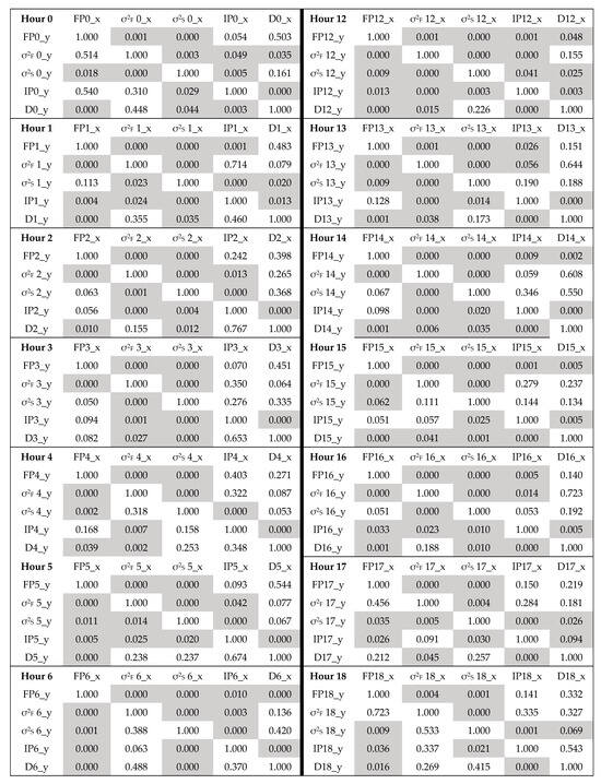
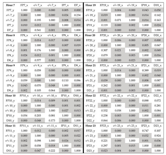
Figure A1.
This figure shows the Granger causality test results, which indicate a likely relationship between time series, with a p-value less than 0.05 indicating a confident rejection of the null hypothesis and that a possible link exists (highlighted cells).

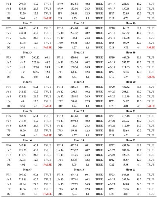
Figure A2.
This figure shows the results of the cointegration test, which identifies a significant link between two or more time series, marked as ‘TRUE’, and non-significant as ‘FALSE’.
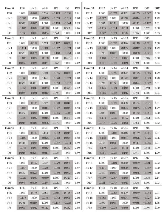
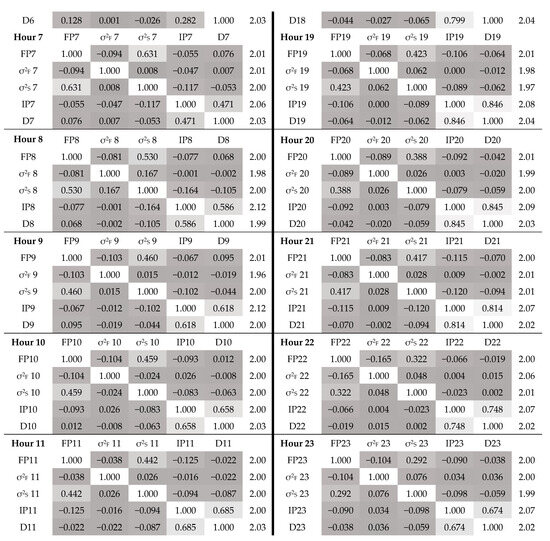
Figure A3.
This figure displays the correlation matrices of the VAR analyses, where stronger correlation is indicated by lighter highlights (and vice versa), and the calculated Durbin–Watson (DW) statistic of each variable, which measures the residual pattern in each time series per cluster, used to test for residual autocorrelations unaccounted for by the VAR model. The DW statistic ranges from 0 to 4, with values closer to 2 indicating no significant correlation.
References
- De Rosa, M.; Gainsford, K.; Pallonetto, F.; Finn, D.P. Diversification, concentration and renewability of the energy supply in the European Union. Energy 2022, 253, 124097. [Google Scholar] [CrossRef]
- Burke, P.J. Income, resources, and electricity mix. Energy Econ. 2010, 32, 616–626. [Google Scholar] [CrossRef]
- Do, T.N.; Burke, P.J. Is ASEAN ready to move to multilateral cross-border electricity trade? Asia Pac. Viewp. 2023, 64, 110–125. [Google Scholar] [CrossRef]
- Chen, F.; Huang, K.; Hou, Y.; Ding, T. Long-term cross-border electricity trading model under the background of Global Energy Interconnection. Glob. Energy Interconnect. 2019, 2, 122–129. [Google Scholar] [CrossRef]
- Oseni, M.O.; Pollitt, M.G. The promotion of regional integration of electricity markets: Lessons for developing countries. Energy Policy 2016, 88, 628–638. [Google Scholar] [CrossRef]
- Haque, H.M.E.; Dhakal, S.; Mostafa, S.M.G. An assessment of opportunities and challenges for cross-border electricity trade for Bangladesh using SWOT-AHP approach. Energy Policy 2020, 137, 111118. [Google Scholar] [CrossRef]
- Dhakal, S.; Karki, P.; Shrestha, S. Cross-border electricity trade for Nepal: A SWOT-AHP analysis of barriers and opportunities based on stakeholders’ perception. Int. J. Water Resour. Dev. 2021, 37, 559–580. [Google Scholar] [CrossRef]
- Thaler, P.; Hofmann, B. The impossible energy trinity: Energy security, sustainability, and sovereignty in cross-border electricity systems. Polit. Geogr. 2022, 94, 102579. [Google Scholar] [CrossRef]
- Yuan, M.; Tapia-Ahumada, K.; Reilly, J. The role of cross-border electricity trade in transition to a low-carbon economy in the Northeastern U.S. Energy Policy 2021, 154, 112261. [Google Scholar] [CrossRef]
- IEA. Mexico—Countries & Regions—IEA. 2024. Available online: https://www.iea.org/countries/mexico/electricity (accessed on 20 February 2024).
- Office of the United States Trade Representative. The United States of America, the United Mexican States, and Canada Trade Agreement 7/1/20 Text|United States Trade Representative. 2023. Available online: https://ustr.gov/trade-agreements/free-trade-agreements/united-states-mexico-canada-agreement/agreement-between (accessed on 20 February 2024).
- Sarmiento, L.; Molar-Cruz, A.; Avraam, C.; Brown, M.; Rosellón, J.; Siddiqui, S.; Rodríguez, B.S. Mexico and U.S. power systems under variations in natural gas prices. Energy Policy 2021, 156, 112378. [Google Scholar] [CrossRef]
- Belize Electricity Limited. Belize Electricity Limited Annual Report 2022. Belize, 2022. Available online: https://indd.adobe.com/view/8fd0b2f4-532b-4a25-b5e8-478794c11a0b (accessed on 26 September 2023).
- Guderjan, T.; Beach, T.; Luzzadder-Beach, S.; Bozarth, S. Understanding the Causes of Abandonment in the Maya Lowlands. Archaeol. Rev. Camb. 2009, 24, 99–121. Available online: https://www.researchgate.net/publication/281572917_Understanding_the_causes_of_abandonment_in_the_Maya_Lowlands (accessed on 6 September 2023).
- IEA. Electricity—Energy System—IEA. 2023. Available online: https://www.iea.org/energy-system/electricity (accessed on 6 September 2023).
- Tillett, A.; Locke, J.; Mencias, J. Belize National Energy Policy Framework. Natl. Energy Policy 2011. Available online: https://www.publicservice.gov.bz/index.php/medias/news-and-events/download/11/56/15 (accessed on 6 September 2023).
- Percino-Picazo, J.C.; Llamas-Terres, A.R.; Viramontes-Brown, F.A. Analysis of Restructuring the Mexican Electricity Sector to Operate in a Wholesale Energy Market. Energies 2021, 14, 3331. [Google Scholar] [CrossRef]
- De la Torre, J.; Rodriguez, L.R.; Monteagudo, F.E.L.; Arredondo, L.R.; Enriquez, J.B. Electricity price forecast in wholesale markets using conformal prediction: Case study in Mexico. Energy Sci. Eng. 2024, 12, 524–540. [Google Scholar] [CrossRef]
- Algieri, B.; Leccadito, A.; Tunaru, D. Risk premia in electricity derivatives markets. Energy Econ. 2021, 100, 105300. [Google Scholar] [CrossRef]
- Wei, W.; Lunde, A. Identifying Risk Factors and Their Premia: A Study on Electricity Prices. J. Financ. Econom. 2022, 21, 1647–1679. [Google Scholar] [CrossRef]
- Fama, E.F. Efficient Capital Markets: A Review of Theory and Empirical Work. J. Financ. 1970, 25, 383. [Google Scholar] [CrossRef]
- Longstaff, F.A.; Wang, A.W. Electricity Forward Prices: A High-Frequency Empirical Analysis. J. Financ. 2004, 59, 1877–1900. [Google Scholar] [CrossRef]
- Koten, S. Van Forward premia in electricity markets: A replication study. Energy Econ. 2020, 89, 104812. [Google Scholar] [CrossRef]
- Ramírez-García, A.; Saucedo, E.; Ramírez-García, A.; Saucedo, E. Hedging Electricity Price Volatility Applying Seasonal and Trend Decomposition. Análisis Económico 2022, 37, 143–166. [Google Scholar] [CrossRef]
- Cruz May, E.; Bassam, A.; Ricalde, L.J.; Escalante Soberanis, M.A.; Oubram, O.; May Tzuc, O.; Alanis, A.Y.; Livas-García, A. Global sensitivity analysis for a real-time electricity market forecast by a machine learning approach: A case study of Mexico. Int. J. Electr. Power Energy Syst. 2022, 135, 107505. [Google Scholar] [CrossRef]
- Rodriguez-Aguilar, R.; Marmolejo-Saucedo, J.A.; Retana-Blanco, B. Prices of Mexican Wholesale Electricity Market: An Application of Alpha-Stable Regression. Sustainability 2019, 11, 3185. [Google Scholar] [CrossRef]
- Livas-García, A.; May Tzuc, O.; Cruz May, E.; Tariq, R.; Jimenez Torres, M.; Bassam, A. Forecasting of locational marginal price components with artificial intelligence and sensitivity analysis: A study under tropical weather and renewable power for the Mexican Southeast. Electr. Power Syst. Res. 2022, 206, 107793. [Google Scholar] [CrossRef]
- Box, G.E.; Jenkins, G.M.; Reinsel, G.C.; Ljung, G.M. Time Series Analysis: Forecasting and Control; John Wiley & Sons: Hoboken, NJ, USA, 2015. [Google Scholar]
- Bollerslev, T. Generalized autoregressive conditional heteroskedasticity. J. Econom. 1986, 31, 307–327. [Google Scholar] [CrossRef]
- Wang, D.; Gryshova, I.; Kyzym, M.; Salashenko, T.; Khaustova, V.; Shcherbata, M. Electricity Price Instability over Time: Time Series Analysis and Forecasting. Sustainability 2022, 14, 9081. [Google Scholar] [CrossRef]
- Ioannidis, F.; Kosmidou, K.; Savva, C.; Theodossiou, P. Electricity pricing using a periodic GARCH model with conditional skewness and kurtosis components. Energy Econ. 2021, 95, 105110. [Google Scholar] [CrossRef]
- Janczura, J.; Puć, A. ARX-GARCH Probabilistic Price Forecasts for Diversification of Trade in Electricity Markets—Variance Stabilizing Transformation and Financial Risk-Minimizing Portfolio Allocation. Energies 2023, 16, 807. [Google Scholar] [CrossRef]
- Ahmad, T.I.; Kiran, K.; Alamgir, A. Households’ Clean Cooking Fuel Poverty: Testing the Energy-Ladder Hypothesis in the Case of Bangladesh. iRASD J. Energy Environ. 2023, 4, 42–55. [Google Scholar] [CrossRef]
- Viehmann, J. Risk premiums in the German day-ahead Electricity Market. Energy Policy 2011, 39, 386–394. [Google Scholar] [CrossRef]
- National Centers for Environmental Information. Past Weather | National Centers for Environmental Information (NCEI). 2024. Available online: https://www.ncei.noaa.gov/access/past-weather/22.16799201091221,-94.84984515217047,16.93260562480587,-84.65998763121615 (accessed on 5 January 2024).
- EIA. Henry Hub Natural Gas Spot Price (Dollars per Million Btu). 2024. Available online: https://www.eia.gov/dnav/ng/hist/rngwhhdD.htm (accessed on 10 January 2024).
- CENACE. Estimation of Actual Demand—Wholesale Electricity Market (MEM). 2024. Available online: https://www.cenace.gob.mx/Paginas/SIM/Reportes/EstimacionDemandaReal.aspx (accessed on 23 February 2024).
- Perktold, J.; Skipper, S.; Taylor, J. Augmented Dickey-Fuller Unit Root-Test, statsmodels.tsa.stattools.adfuller—statsmodels 0.15.0 (+213); 2024. Available online: https://www.statsmodels.org/dev/generated/statsmodels.tsa.stattools.adfuller.html (accessed on 28 February 2024).
- Dickey, D.A.; Fuller, W.A. Likelihood Ratio Statistics for Autoregressive Time Series with a Unit Root. Econometrica 1981, 49, 1057. [Google Scholar] [CrossRef]
- Smith, T.G. pmdarima 2.0.4 API Reference, pmdarima.arima.auto_arima—pmdarima 2.0.4 documentation; 2023. Available online: https://alkaline-ml.com/pmdarima/modules/generated/pmdarima.arima.auto_arima.html (accessed on 28 February 2024).
- Breusch, T.S.; Pagan, A.R. The Lagrange Multiplier Test and its Applications to Model Specification in Econometrics. Rev. Econ. Stud. 1980, 47, 239. [Google Scholar] [CrossRef]
- Nugroho, D.B.; Priyono, A.; Susanto, B. Skew normal and skew student-t distributions on GARCH(1,1) model. Media Stat. 2021, 14, 21–32. [Google Scholar] [CrossRef]
- Hacker, R.S.; Hatemi-J, A. Optimal lag-length choice in stable and unstable VAR models under situations of homoscedasticity and ARCH. J. Appl. Stat. 2008, 35, 601–615. [Google Scholar] [CrossRef]
- statsmodels 0.14.1. Time Series Analysis Tsa—statsmodels 0.14.1. 2024. Available online: https://www.statsmodels.org/stable/tsa.html (accessed on 19 April 2024).
- Durbin, J.; Watson, G.S. Testing for serial correlation in least squares regression. I. Biometrika 1950, 37, 409–428. [Google Scholar] [CrossRef] [PubMed]
- Granger, C.W.J. Investigating Causal Relations by Econometric Models and Cross-spectral Methods. Econometrica 1969, 37, 424. [Google Scholar] [CrossRef]
- Johansen, S. Estimation and Hypothesis Testing of Cointegration Vectors in Gaussian Vector Autoregressive Models. Econometrica 1991, 59, 1551. [Google Scholar] [CrossRef]
- Valitov, N. Risk premia in the German day-ahead electricity market revisited: The impact of negative prices. Energy Econ. 2019, 82, 70–77. [Google Scholar] [CrossRef]
- Bessembinder, H.; Lemmon, M.L. Equilibrium Pricing and Optimal Hedging in Electricity Forward Markets. J. Finance 2002, 57, 1347–1382. [Google Scholar] [CrossRef]
Disclaimer/Publisher’s Note: The statements, opinions and data contained in all publications are solely those of the individual author(s) and contributor(s) and not of MDPI and/or the editor(s). MDPI and/or the editor(s) disclaim responsibility for any injury to people or property resulting from any ideas, methods, instructions or products referred to in the content. |
© 2024 by the authors. Licensee MDPI, Basel, Switzerland. This article is an open access article distributed under the terms and conditions of the Creative Commons Attribution (CC BY) license (https://creativecommons.org/licenses/by/4.0/).