Enhancing Oil Recovery Predictions by Leveraging Polymer Flooding Simulations and Machine Learning Models on a Large-Scale Synthetic Dataset

Abstract

Polymer flooding is a prominent enhanced oil recovery process that is widely recognized for its cost-effectiveness and substantial success in increasing oil production. In this study, the Buckley–Leverett mathematical model for polymer flooding was used to generate more than 163,000 samples that reflect different reservoir conditions using seven input parameters. We introduced artificial noise into the dataset to simulate real-world conditions and mitigate overfitting. Seven classic machine learning models and two neural networks were trained on this dataset to predict the oil recovery factor based on the input parameters. Among these, polynomial regression performed best with a coefficient of determination ($R^2$) of 0.909, and the dense neural network and cascade-forward neural network achieved $R^2$ scores of 0.908 and 0.906, respectively. Our analysis included permutation feature importance and metrics analysis, where key features across all models were identified, and the model’s performance was evaluated on a range of metrics. Compared with similar studies, this research uses a significantly larger and more realistic synthetic dataset that explores a broader spectrum of machine learning models. Thus, when applied to a real dataset, our methodology can aid in decision-making by identifying key parameters that enhance oil production and predicting the oil recovery factor given specific parameter values.

1. Introduction

Enhancing oil recovery, especially as the effectiveness of conventional waterflooding wanes, is becoming increasingly critical in sustaining global energy supplies. Our research directly addresses the urgent need for more accurate predictions of oil recovery rates through the use of polymer flooding, a preferred tertiary recovery strategy when other methods plateau in effectiveness [1,2]. By leveraging a large-scale synthetic dataset generated with the Buckley–Leverett model for polymer flooding, supplemented with introduced noise, this study aimed to answer the following questions: (a) can machine learning models effectively learn patterns within these complex data, and (b) what are the most suitable types of machine learning models—be it parametric, non-parametric, ensemble methods, or neural networks—for this dataset? The outcomes could significantly influence both the technical and economic aspects of enhanced oil recovery.

To emphasize the potential impact of advancements in polymer floodings, a review of previous studies offers valuable insights. The analysis of 55 polymer flooding projects in China’s Daqing Oil Field, conducted between 1991 and 2014, revealed incremental oil recovery rates ranging from 1.9% to 19.5% of original oil in place. This comprehensive study utilized advanced statistical and graphical techniques to assess the effectiveness of polymer flooding as an enhanced oil recovery (EOR) method. Insights into crucial factors such as polymer properties, well configurations, and other operational variables were gathered, highlighting the potential for optimizing EOR strategies. This significant research was conducted by Zhang et al. [3]. Within the field of EOR, the complexity and high dimensionality of reservoir simulations necessitate extensive computational resources and time due to the need to handle numerous input parameters like porosity, permeability, and multi-phase flow functions.

The adoption of data-driven proxy models, leveraging simplified inputs and machine learning algorithms like artificial neural networks (ANN), is increasing in enhanced oil recovery (EOR) operations. These models enable the swift evaluation of operational scenarios to optimize production and develop fields efficiently, managing uncertainties related to reservoir heterogeneities and operational constraints. This approach reduces computational demands and enhances decision-making efficiency. Studies demonstrate ANN’s effectiveness in analyzing reservoir characteristics, forecasting well performance, and predicting oil production [4,5,6,7,8,9,10]. Moreover, further research has shown the effectiveness of machine learning in analyzing chemical flooding. Karambeigi et al. [11] developed a multilayer perceptron (MLP) model for predicting recovery factor (RF) and net present value (NPV) in chemical flooding using surfactants and polymers, with data from Prasanphanich’s thesis [12] on Benoist sand reservoir simulations. This MLP utilized the following seven input parameters: surfactant slug size, polymer drive size, surfactant concentration, the salinity of polymer drive, the Kv/Kh ratio, and polymer concentration in polymer drive and surfactant slug. Furthermore, it demonstrated a high accuracy, with prediction errors below 5%. Additionally, Al-Dousari et al. [13] created an ANN model using data from 624 simulations with 18 input parameters, achieving an average absolute error of about 3% in predicting oil recovery for 125 test cases.

The study by Alkhatib et al. [14] employed the least squares Monte Carlo (LSM) method in surfactant flooding scenarios to address uncertainties in both technical and economic parameters using both 3D homogeneous and 2D heterogeneous reservoir models. The findings revealed that implementing the Monte Carlo LSM with surfactants offers flexibility in handling uncertainty and mitigating associated challenges. Ahmadi et al. [15] applied a genetically enhanced least squares support vector machine (LSSVM) to chemical flooding, achieving a high correlation coefficient of 0.993 using the same dataset as Karambeigi et al. [11]. Jahani-Keleshteri [16] and Le Van et al. [17] utilized LSSVM and ANN techniques, respectively, for different aspects of oil production, with Le Van et al.‘s ANN showing a mean squared error of 1.63% in ASP flooding in China’s Gudong oil field [1]. Larestani et al. [18] explored various intelligent models like cascade-forward neural network (CFNN) and radial basis function (RBF) for surfactant–polymer flooding on Prasanphanich’s [12] experimental dataset consisting of 202 data points, finding the CFNN-LM (Levenberg–Marquardt) model to be highly accurate, with a 0.66% error in predicting recovery factor. Mohammadi et al. [19] further demonstrated the effectiveness of cascade-forward neural networks in optimizing thermal-enhanced oil recovery processes.

Regarding polymer flooding, Ebaga-Ololo and Chon [20] utilized a dataset from their previous study [21] comprising reservoir data and polymer concentrations to train an ANN, achieving high accuracy, with a maximum root mean squared error of about 0.36%. Alghazal [22] explored ANN models for water and polymer flooding in naturally fractured reservoirs, focusing on both forward and inverse problems. Norouzi et al. developed a workflow utilizing static proxy models for optimizing Disproportionate Permeability Reduction (DPR) polymer gel treatments to reduce water production and improve economic outcomes [23]. Amirian et al. used backpropagation and Levenberg–Marquardt neural networks for polymer flooding forecasting in heavy oil reservoirs, finding the latter particularly effective [24]. Finally, Sun and Ertekin introduced a novel approach for optimizing polymer flooding projects using both forward-looking and inverse-looking ANN models. These models utilize synthetic production histories generated from high-fidelity numerical simulations to predict time-based project responses and optimal project design schemes, respectively. Extensive testing confirmed the reliability of these models in real-world applications [25].

After reviewing various approaches for modeling polymer flooding, it becomes apparent there is still a need for more comprehensive datasets that capture a broader range of reservoir conditions and variables. This study addresses the gap by employing the Buckley–Leverett model for the polymer flooding problem to generate an extensive dataset of over 163,000 samples. This dataset reflects diverse reservoir conditions with detailed parametric information, such as oil and water viscosity, absolute permeability, porosity, pressure, polymer concentration, and oil and water saturation. To enhance predictive capabilities and operational insights for polymer flooding, this study applied nine machine learning methods—linear regression, polynomial regression, decision trees, random forest, gradient boosting, extreme gradient boosting, light gradient boosting, dense neural networks, and cascade-forward neural networks—to the dataset generated using the Buckley–Leverett model. By employing these machine learning algorithms, this study seeks to determine the most effective machine learning strategies for predicting recovery factors under different reservoir conditions and parameters.

2. Materials and Methods

2.1. Dataset

The dataset in our study was produced by simulating the Buckley–Leverett mathematical model for polymer flooding [26,27] across a range of oil reservoir parameter values. The mathematical model was solved implicitly and iteratively to generate a dataset comprising 163,726 data points. The features of the dataset are absolute permeability, pressure, porosity, oil saturation, water saturation, oil viscosity and polymer concentration. The target variable is the oil recovery factor. The mathematical model outputs for oil and water saturation, pressure, and polymer concentration were vectors, as they described different points of the reservoir. To adapt these data for tabular representation, the average values of these vectors were calculated.

The statistical summary of the dataset is shown in

Table 1. Statistical summary of the generated dataset.

Variables	Variable Type	Mean	Std	Min	Max
Absolute permeability (k)	Feature	0.004	0.002	0.001	0.008
Pressure (P)	Feature	0.305	0.004	0.301	0.335
Porosity (m)	Feature	0.454	0.147	0.2	0.705
Oil saturation (So)	Feature	0.934	0.075	0.0003	0.993
Water saturation (Sw)	Feature	0.066	0.075	0.007	0.999
Oil viscosity (μ)	Feature	0.453	0.089	0.3	0.605
Polymer concentration (Cp)	Feature	0.045	0.029	0.006	0.172
Oil recovery factor (RF)	Target	0.066	0.075	0.007	0.999

.

There existed a significant correlation between the variables in the dataset. The oil recovery factor exhibited significant correlations with several variables, as seen in the correlation matrix in Figure 1. Notably, it was perfectly negatively correlated (−1.00) with oil saturation, suggesting an inverse relationship: as one increased, the other decreased. Moreover, there was a perfect positive correlation (1.00) with the water saturation, indicating that they could increase or decrease together in a linear fashion. The moderate positive correlation of the other variables indicates that these variables influence the oil recovery factor to some extent. The existence of strong correlations between the features and the target variable is beneficial for training models with high accuracy.

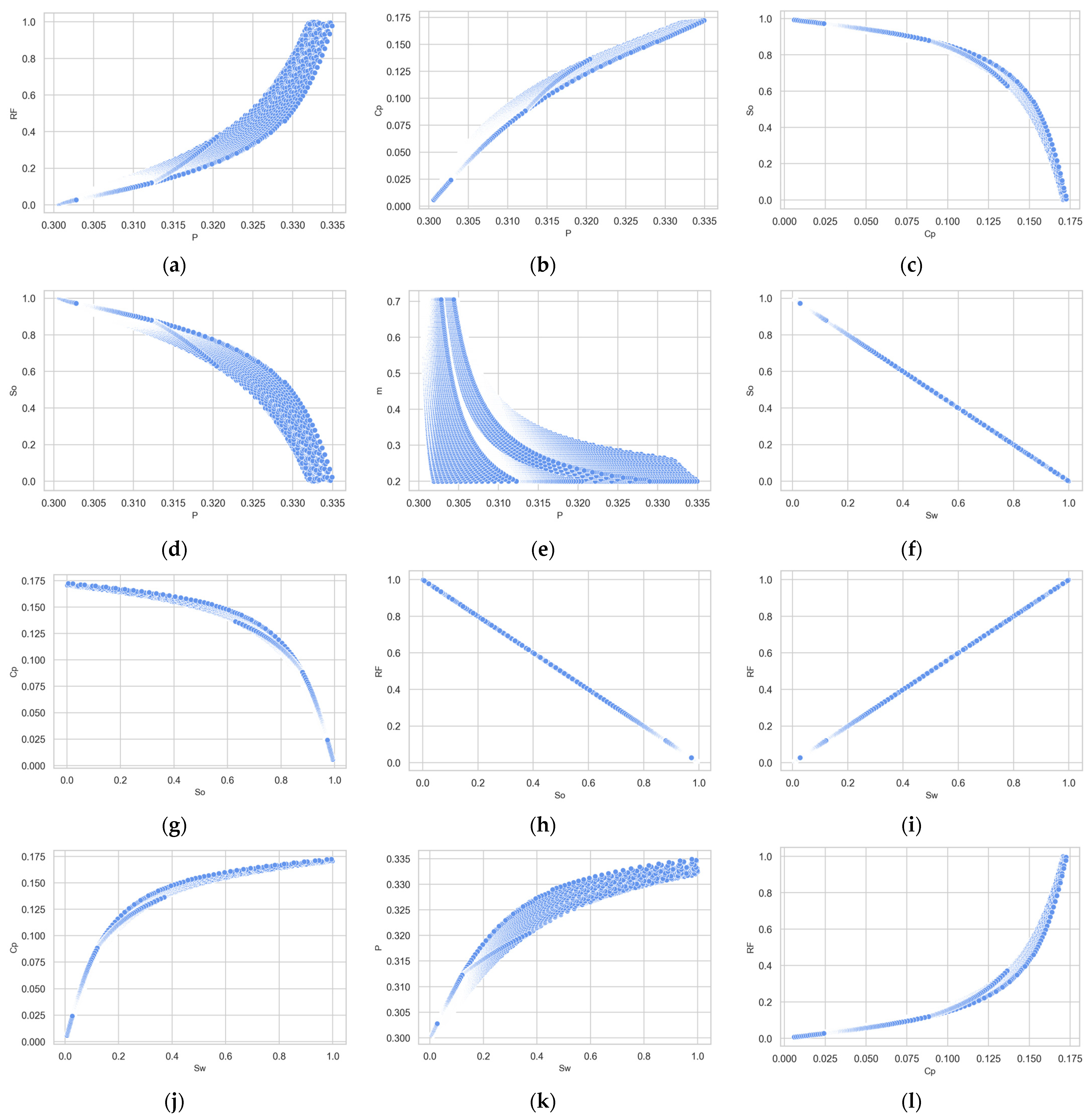
Moreover, there are diverse interactions among key variables in the dataset. This can be seen in the pairwise scatter plot between key variables in Figure 2. Some pairs of variables do not exhibit a discernible relationship, which indicates a lack of direct correlation or a more complex underlying interaction that cannot be captured through simple two-dimensional scatter plots. These pairs were not included in the pair plot. Noteworthy are the positive non-linear relationships observed between pressure and recovery factor, polymer concentration and recovery factor, polymer concentration and water saturation, and pressure and polymer concentration. These non-linear trends suggest that as one variable increases, the effect on the other variable accelerates, which is indicative of threshold effects or synergistic interactions.

In contrast, negative non-linear relationships existed between oil saturation and pressure and polymer concentration and oil saturation, where increases in one variable corresponded to disproportionate decreases in the other. This reflects diminishing effects under certain conditions.

Linear relationships were also present; water saturation and recovery factor had a positive linear relationship, suggesting a direct proportionality between these variables—increases in water saturation consistently corresponded to increases in recovery factor. Conversely, water saturation and oil saturation, along with oil saturation and recovery factor, showed negative linear relationships, indicating an inverse proportionality.

2.2. Adding Artificial Noise

The synthetic dataset that was generated is ideal, containing no noise or distortions, unlike real data. Previous studies have shown that machine learning models trained on synthetic datasets often fail to capture appropriate relationships present in real data and, therefore, perform poorly on real-world data [28,29]. These models show deceptively high performance on both training and testing with synthetic data. In our initial experiments, our models exhibited significant overfitting when training on the noise-free dataset, achieving near-perfect scores across various regression metrics. To mitigate this, artificial noise was introduced to the dataset to better simulate real-world scenarios and increase the complexity of the learning challenge. This approach encourages the model to capture more complex relationships and avoid overfitting.

In this study, Gaussian noise was utilized. Gaussian noise is statistical noise having a probability density function (PDF) equal to that of the normal distribution. In other words, it is noise that follows a bell-shaped curve in its amplitude distribution. Mathematically, it is characterized by two parameters: the mean ($\mu$) and the standard deviation ($\sigma$). The formula for the PDF of a Gaussian distribution is given by the following:

$$f\left(x\right|\mu ,\sigma )=\frac{1}{\sigma \sqrt{2\pi }}\exp \left(-\frac{{\left(x-\mu \right)}^2}{2{\sigma }^2}\right),$$

where $x$ is the variable, $\mu$ is the mean (or expectation of the distribution), $\sigma$ is the standard deviation, and ${\sigma }^2$ is the variance.

When adding noise to data, the mean and the standard deviation are prominent parameters. The mean ($\mu$) of the Gaussian noise is usually set to zero, meaning that the noise, on average, does not lean toward positive or negative values and, therefore, does not bias the data. The standard deviation ($\sigma$) controls the variability or spread of the noise. A larger value of σ means that the noise can cause larger perturbations in the data. This is a very important parameter for our problem.

In our study, the noise was drawn from a normal distribution with a mean of zero, and the standard deviation was set to 30% of the standard deviation values of each column (variable). After adding this noise to the original dataset, a modified version that retained the underlying relationships but included controlled distortions was obtained. As seen in Figure 3, the correlation between the variables was not significantly affected by the noise, although there are noticeable differences. There still existed a strong negative correlation with oil saturation and a strong positive correlation with water saturation. Despite the introduction of noise, key predictive relationships in the data were robust.

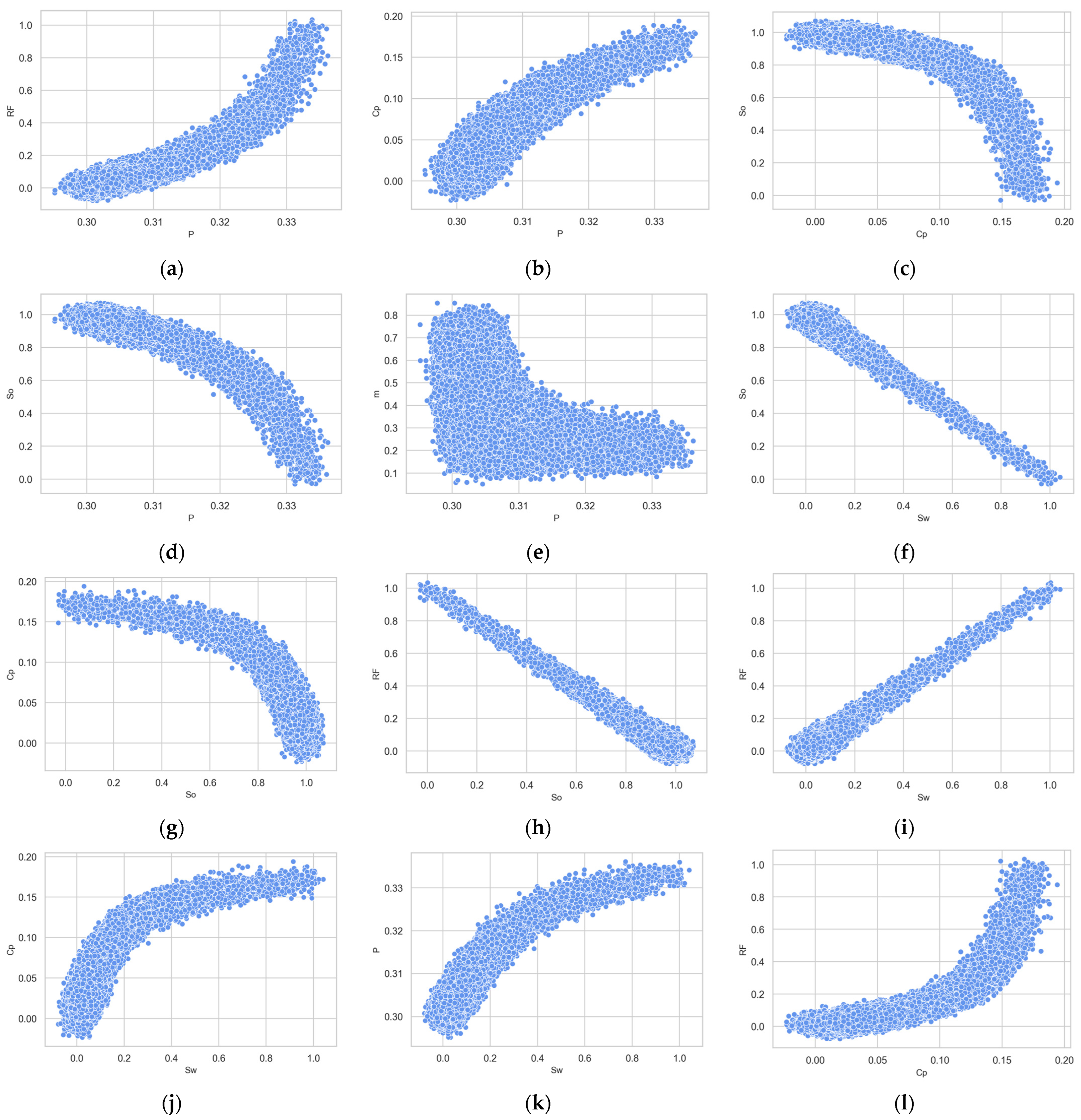
In addition, it can be observed that the relationship between these variables was maintained after introducing artificial noise, although with some distortion, as illustrated in Figure 4. This added complexity increases the challenge of model training but also fosters the development of more capable models. Such models demonstrate their capability to manage real-world scenarios, affirming that machine learning models are able to learn on real-world, noisy datasets to predict RF, thereby enhancing their practical applicability and reliability in the oil and gas industry.

2.3. Machine Learning Algorithms

After introducing artificial noise, the dataset was partitioned into features and targets, as seen in Table 1. In this study, nine different machine learning models were explored. Seven are classic algorithms: linear regression, polynomial regression, decision tree, random forest, gradient boosting, extreme gradient boosting, and light gradient boosting. The remaining two are neural network architectures: dense neural network and cascade-forward neural network.

For model training, the dataset was split into 70% training and 30% testing for the classic algorithms. For the neural networks, 70% was used for training, with 30% of that reserved for validation and the remaining 30% for testing. The scikit-learn library was used for the classic models, TensorFlow for the dense neural network, and MATLAB 9.4 (R2018a) for the cascade-forward neural network.

The train and test set were split randomly. This ensured that the training and testing sets were independent of each other, and given the relatively large size of our dataset, this method provided an adequate representation of the overall data distribution in both sets. Moreover, this led to an unbiased evaluation of the model’s performance.

2.3.1. Linear Regression (LR)

The scikit-learn implementation of LR uses the ordinary least squares method, which employs the normal equation to find the coefficients that minimize the loss function. The formula of LR is given as follows:

$$y={\beta }_0+{\beta }_1{x}_1+\dots +{\beta }_n{x}_n$$

Each $x_i$ represents a different independent variable (the seven features), and each ${\beta }_i$ is the coefficient for the corresponding $x_i$. ${\beta }_0$ is the intercept term, otherwise known as the bias. These coefficients provide information on the model’s decision-making and about the feature importance [30].

2.3.2. Polynomial Regression (PR)

PR is another form of LR in which the relationship between the independent variables $x$ (features) and the dependent variable $y$ (RF) are modeled as an $n$th degree polynomial. Polynomial regression fits a non-linear relationship between the value of $x$and the expected value of $y.$The general form of a polynomial regression of degree $n$ is the following:

$$y={\beta }_0+{\beta }_{11}{x}_1+{\beta }_{12}{x}_1^2+{\beta }_{1m}{x}_1^m+{\beta }_{2n}{x}_2^n+\dots +{\beta }_{kp}{x}_k^p,$$

where $y$ is the target variable, $x_1,\dots ,x_k$ are the features, ${\beta }_0$ is the bias term, and ${\beta }_{ij}$ is the coefficient for the $j\mathrm{t}\mathrm{h}$ power of the $i\mathrm{t}\mathrm{h}$ feature. $m,n,\dots ,p$ are the highest polynomial degree for the respective features.

Each ${\beta }_{ij}{x}_i^j$ represents the contribution of the $j$th power of the $i$th feature to the predicted variable $y.$ The main advantage of PR is that it gives the model flexibility to capture non-linear relationships that might exist between the features. In this study, Sci-kit Learn’s PolynomialFeatures and GridSearchCV were used to determine the optimal polynomial degree [30].

2.3.3. Decision Tree (DT)

The DT algorithm is a non-parametric machine learning method, meaning that it does not make assumptions about the underlying data or the linear relationship of the features, unlike parametric methods such as LR [31].

A DT consists of decision nodes and leaf nodes (decision outcomes). The core algorithm for building decision trees is called CART (Classification and Regression Tree). To build a tree, a DT splits each node on the feature and threshold, which results in the largest reduction variance.

The variance ${\sigma }^2$ of a node $D$ in a decision tree is calculated using the following:

$${\sigma }^2\left(D\right)=\frac{1}{\left|D\right|}{\sum }_{i=1}\left|D\right|+\left(y_i-{\overline{y}}_i\right),$$

where $\left|D\right|$ is the number of samples at node $D$, $y_i$ are the target values of the samples in $D$, and $\overline{y}$ is the mean of the target values in $D$.

To calculate the reduction in variance, the formula below is used:

$$ReductioninVariance={\sigma }^2\left(D\right)-\left(\frac{\left|D_{left}\right|}{\left|D\right|}{\sigma }^2\left(D_{left}\right)+\frac{\left|D_{right}\right|}{\left|D\right|}{\sigma }^2\left(D_{right}\right)\right)$$

here, ${\sigma }^2(D)$ is the variance of the parent node before the split, and ${\sigma }^2\left(D_{left}\right)$ and ${\sigma }^2\left(D_{right}\right)$ are the variances of the left and right nodes, respectively. $\left|D_{left}\right|\mathrm{a}\mathrm{n}\mathrm{d}\left|D_{right}\right|$ are the number of samples in the left and right nodes. $\left|D\right|$ is the total number of samples in the parent node.

The goal is to choose a split that maximizes the reduction in variance. This criterion assumes that a greater decrease in variance yields more homogenous subsets, which is desirable as it implies that the predictions within each subset are more accurate and less spread out.

The algorithm starts at the root node of the tree and then recursively splits the node into child nodes. However, this often leads to overfitting; therefore, several stopping criteria (hyperparameters) are used. These include the maximum depth of the tree, the minimum number samples required to split an internal node, and the minimum number of samples required to be at a leaf node, among others. In this study, GridSearch CV was utilized to find the optimal values of these hyperparameters.

2.3.4. Random Forest Regressor (RFR)

RFR is an ensemble learning method that constructs multiple DTs during training. Each tree in an RFR is built from a sample drawn with replacement, known as the bootstrap sample, from the training set. When growing each tree, RFR introduces additional randomness; when splitting a node, it selects a random subset of features to consider. The overall prediction by the RFR is made by averaging the predictions of the individual trees. RFR helps mitigate the problem of overfitting often faced by DTs and leads to better predictive accuracy [32].

For regression tasks, the prediction of an RFR model can be summarized by the average of the predictions from all the individual trees in the forest:

$$y=\frac{1}{T}{\sum }_{t=1}{h}_t\left(x\right),$$

where $y$is the predicted output, $T$ is the total number of trees in the forest, $h_t\left(x\right)$ is the prediction from the tth tree, and $x$ is the input feature vector.

2.3.5. Gradient Boosting (GB)

GB is another ensemble learning method that can be used for regression tasks. It builds on the concept of boosting, where multiple weak learners (in our study, DTs) are combined to create a strong predictive model. GB models are trained iteratively, with each new model built to correct errors made by the previous models in the ensemble. Unlike traditional gradient descent, which updates the model parameters directly, GB updates the model by successfully adding new models that correct the residuals or errors of the previous models [33].

The general update formula for GB can be summarized as follows:

$$F_t\left(x\right)=F_{t-1}\left(x\right)+v\cdot {\gamma }_t\cdot h_t\left(x\right),$$

where $F_t\left(x\right)$ is the model at iteration t, $F_{t-1}\left(x\right)$is the model from the previous iteration, $v$is the learning rate that scales the contribution of each tree, and ${\gamma }_t$ is the optimal multiplier for the $t$th tree found by multiplying the loss when this tree is added to the ensemble, and $h_t\left(x\right)$ is the output of the $t\mathrm{t}\mathrm{h}$tree, which is fitted on the residuals of the model at $t-1$.

2.3.6. Extreme Gradient Boosting (XGBoost)

XGBoost is a highly efficient implementation of GB due to its performance and speed. It enhances GB by incorporating regularization, which helps with overfitting and improves model generalization. It is initialized with a simple model and is improved incrementally. The trees are built using a gradient descent algorithm that minimizes a loss function defined to include a regularization term. In each iteration, XGBoost computes the gradients of the loss function with respect to predictions made by the current model [34].

One of the main differentials of XGBoost is its objective function, defined below:

$$Obj\left(\theta \right)=L\left(\theta \right)+\mathsf{\Omega }(\theta ),$$

where $L\left(\theta \right)$ represents the traditional loss function, which measures how predictive the model is with respect to the actual data, and $\mathsf{\Omega }\left(\theta \right)$ represents the regularization term, which could be the sum of weights squared (L2 norm) or the sum of absolute weights (L1 norm), plus the complexity of the trees, such as the number of leaves.

2.3.7. Light Gradient Boosting (LightGBM)

LightGBM is a very efficient GB variation that uses tree-based learning algorithms with a leaf-wise growth strategy. The algorithm reduces training time and improves model accuracy. Specifically, it uses histogram-based algorithms for optimal splits, which reduces memory consumption. For our regression analysis, LightGBM’s gradient-based one-side sampling (GOSS) and exclusive feature bundling (EFB) were particularly beneficial [35].

2.3.8. Dense Neural Networks (DNNs)

DNNs are machine learning methods loosely inspired by the information-processing patterns found in the human brain. DNNs have interconnected neurons, where each neuron in a layer is connected to every neuron in the subsequent layer. DNNs process information by responding to external inputs and passing their output to subsequent layers of neurons [36]. A typical architecture of a DNN consists of three main layers: the input layer, one or more hidden layers, and the output layer. The strength of the connection of each neuron in these layers to all neurons in the next layer is represented by weights $\left(w_i\right)$ that are adjusted during training.

In a DNN, each neuron computes a linear combination of its inputs, represented by the following:

$$f\left(x\right)={\sum }_{i=1}^n{w}_i{x}_i+b,$$

where $w_i$ are the weights, $x_i$are the inputs, and $b$ is a bias. This sum $f(x)$ is then fed into a non-linear activation function, in our case, the Rectified Linear Unit (ReLU) activation function, which is calculated as $ReLU\left(x\right)=\mathrm{m}\mathrm{a}\mathrm{x}(0,f(x))$ [37]. The output of the ReLU function is what is passed on to the next layer or used to calculate the output of the network.

The training of DNNs involves adjusting the weights of the connections to minimize the error between the predicted and actual outputs. This is done using backpropagation and gradient descent. Backpropagation calculates the gradient of the loss function with respect to each weight in the network, and gradient descent uses this information to update the weights in a direction that reduces the error.

In our study, a model with three hidden layers containing 256, 128, and 64 neurons, respectively, was constructed. The ReLU activation function was utilized across the hidden layers, and a linear activation function ($f\left(x\right)=x)$ was used for the output layer. The network underwent training for 200 epochs with a batch size of 512. The selection of these parameters was guided by heuristics and iterative trial-and-error. The architecture of DNN is depicted in Figure 5.

2.3.9. Cascade-Forward Neural Networks (CFNN)

A CFNN is a type of ANN that closely resembles feedforward networks, but it includes connections from the input and all preceding layers to subsequent layers. In a network with three layers, the output layer is directly connected not only to the hidden layer but also to the input layer. The advantage of this approach is that it accounts for the non-linear relationship between input and output while preserving their linear relationship [38].

In this research, a model constructed with two hidden layers consisting of 15 hidden neurons for the first layer and five neurons for the second layer gave optimal results. The activation functions used were the Tansig (tanh) for the hidden layers and Purelin (linear) for the output layer. The Levenberg–Marquardt method, known for its superior performance in non-linear optimization, was employed to train the model. The selection of these parameters was guided by heuristics and iterative trial-and-error. The architecture of the developed CFNN model is illustrated in Figure 6. In the diagram, ‘W’ and ‘b’ represent the weights and biases of the neural network. The numbers (7, 15, 5, 1) indicate the number of neurons in the input, first hidden, second hidden, and output layers, respectively.

2.4. Metrics

To evaluate our regression models, four metrics were chosen, namely mean absolute error, root mean squared error, R-squared, and mean absolute percentage error.

2.4.1. Root Mean Squared Error (RMSE)

RMSE is the square root of the mean of the squared errors. The RMSE measures the average magnitude of the error. It is especially useful when large errors are particularly undesirable. The square root in RMSE provides it the same units as the target variable, making interpretation straightforward [39]. Lower RMSE values indicate a better fit. The formula of RMSE is the following:

$$RMSE=\sqrt{\frac{1}{n}\sum _{i=1}^n{\left(y_i-{\widehat{y}}_i\right)}^2}$$

2.4.2. Mean Absolute Error (MAE)

MAE is a statistical measure to evaluate the performance of regression models. It represents the average magnitude of errors between predicted and actual values without considering their direction (signs). MAE provides a linear score, meaning that all individual differences are weighted equally in the average. This makes it resistant to outliers. The formula for MAE is the following:

$$MAE=\frac{1}{n}\sum _{i=1}^n\left|y_i-{\widehat{y}}_i\right|$$

2.4.3. Coefficient of Determination $({\mathrm{R}}^2)$

$R^2$, also known as the coefficient of determination, measures the proportion of variance in the dependent variable that is predictable from the independent variable. It is a statistical measure of how well the regression predictions approximate the real data points. An $R^2$ of 1 indicates that the regression predictions perfectly fit the data. The formula for $R^2$ is the following:

$$R^2=1-\frac{\sum _{i=1}^n{\left(y_i-\widehat{y_i}\right)}^2}{\sum _{i=1}^n{\left(y_i-\overline{y}\right)}^2},$$

where $\overline{y}$ is the mean of y values.

2.4.4. Mean Absolute Percentage Error (MAPE)

MAPE expresses the error as a percentage and measures the average magnitude of the errors in a set of predictions without considering their direction (signs). It is particularly useful when it is imperative to explain the accuracy of the model in percentage terms. Lower values of MAPE indicate better predictive accuracy. The formula of MAPE is the following:

$$MAPE=100\frac{1}{n}\sum _{t=1}^n\left|\frac{y_i-{\widehat{y}}_i}{y_i}\right|$$

3. Results and Discussion

In this study, we evaluated the performance of nine different machine learning models trained to predict the oil recovery factor based on the following parameters: absolute permeability, pressure, porosity, oil saturation, water saturation, oil viscosity, and polymer concentration. Of these models, seven were classic algorithms: LR, PR, DT, RFR, GB, XGBoost, and LightGBM. The remaining two were neural networks: DNN and CFNN. The classic models were assessed using four key metrics: RMSE, MAE, $R^2$, and MAPE. In contrast, the ANNs were assessed using three metrics: RMSE, MAE, and $R^2$. Moreover, permutation feature importance analysis was conducted to identify the key features that influence the decision-making process of the models.

3.1. Model Evaluation Results

As detailed in

Table 2. Multi-metric evaluation results of classic trained models.

	Metrics	LR	PR	DT	RFR	GB	XGBoost	LightGBM
Train Set	RMSE	0.027	0.024	0.024	0.013	0.027	0.024	0.023
	MAE	0.021	0.019	0.019	0.011	0.021	0.019	0.018
	$R^2$	0.885	0.91	0.907	0.971	0.883	0.907	0.914
	MAPE	2.948	3.075	3.014	1.943	3.872	3.082	2.98
Test set	RMSE	0.026	0.024	0.025	0.024	0.027	0.024	0.025
	MAE	0.021	0.019	0.02	0.019	0.021	0.019	0.019
	$R^2$	0.886	0.909	0.9	0.905	0.882	0.902	0.901
	MAPE	2.614	2.508	2.639	2.511	3.331	2.565	2.494

and

Table 3. Multi-metric evaluation results of trained ANNs.

	Metrics	DNN	CFNN
Train Set	RMSE	0.024	0.024
	MAE	0.019	0.019
	$R^2$	0.909	0.911
Test set	RMSE	0.024	0.024
	MAE	0.019	0.019
	$R^2$	0.908	0.906

, our results indicate that the PR and the RFR models outperformed the others across most metrics. Notably, these models achieved the highest $R^2$values on the test set, suggesting a strong ability to generalize beyond the training data. Table 2 provides a detailed evaluation of the classic machine learning models used in our study, presenting the results across the four metrics chosen for both the training and testing set.

Similarly, Table 3 presents the performance outcomes for DNN and CFNN.

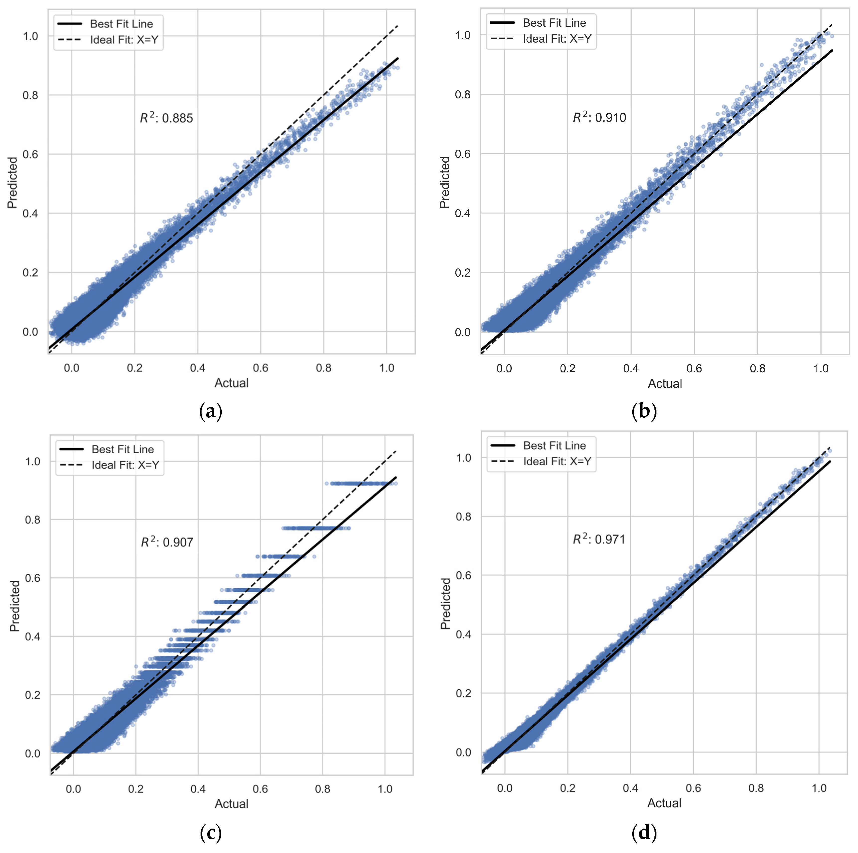
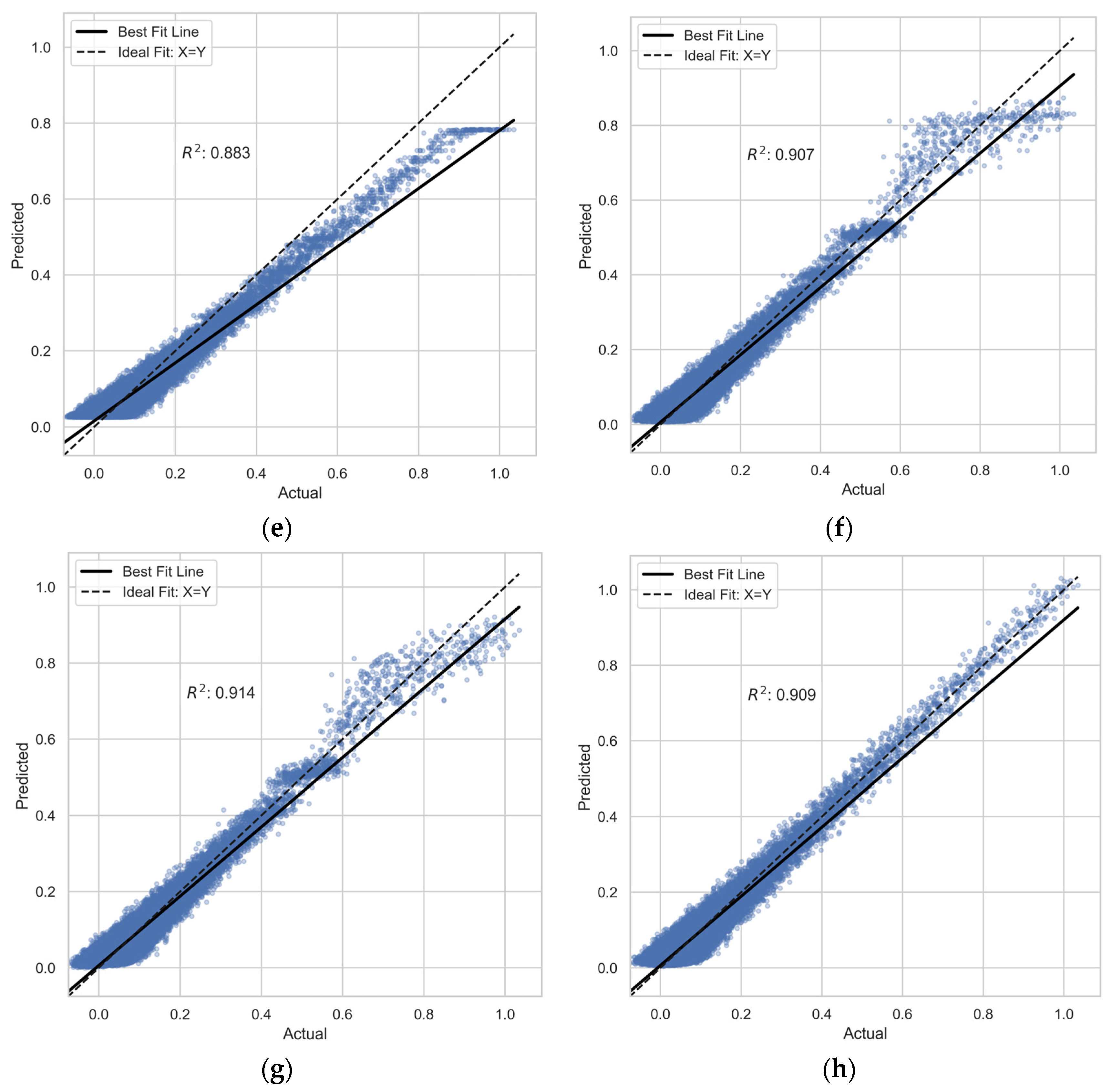
To visually compare the training and testing performance of the models, plots of actual versus predicted values were used, with $R^2$ as the evaluation metric. Figure 7 illustrates the performance of the regression models on training data; the predictive accuracy and trend of predictions can be visually assessed by the proximity of data points to the identity line (Y = X), which represents perfect prediction. The blue dots represent actual training data values against the predicted values as a scatter plot. Additionally, the best-fit line in the plot illustrates the empirical relationship derived from the model. This line helps to evaluate the model’s prediction trend; the closer this line is to the identity line, the better the model’s predictive performance and the lower the bias.

The RFR model performed best on the training set with $R^2$ of 0.971. Similarly, LightGBM, PR, and XGBoost exhibited strong fits, with $R^2$values of 0.914, 0.910, and 0.907, respectively. The GB and LR models are slightly less accurate, showing $R^2$ values of 0.883 and 0.885, respectively.

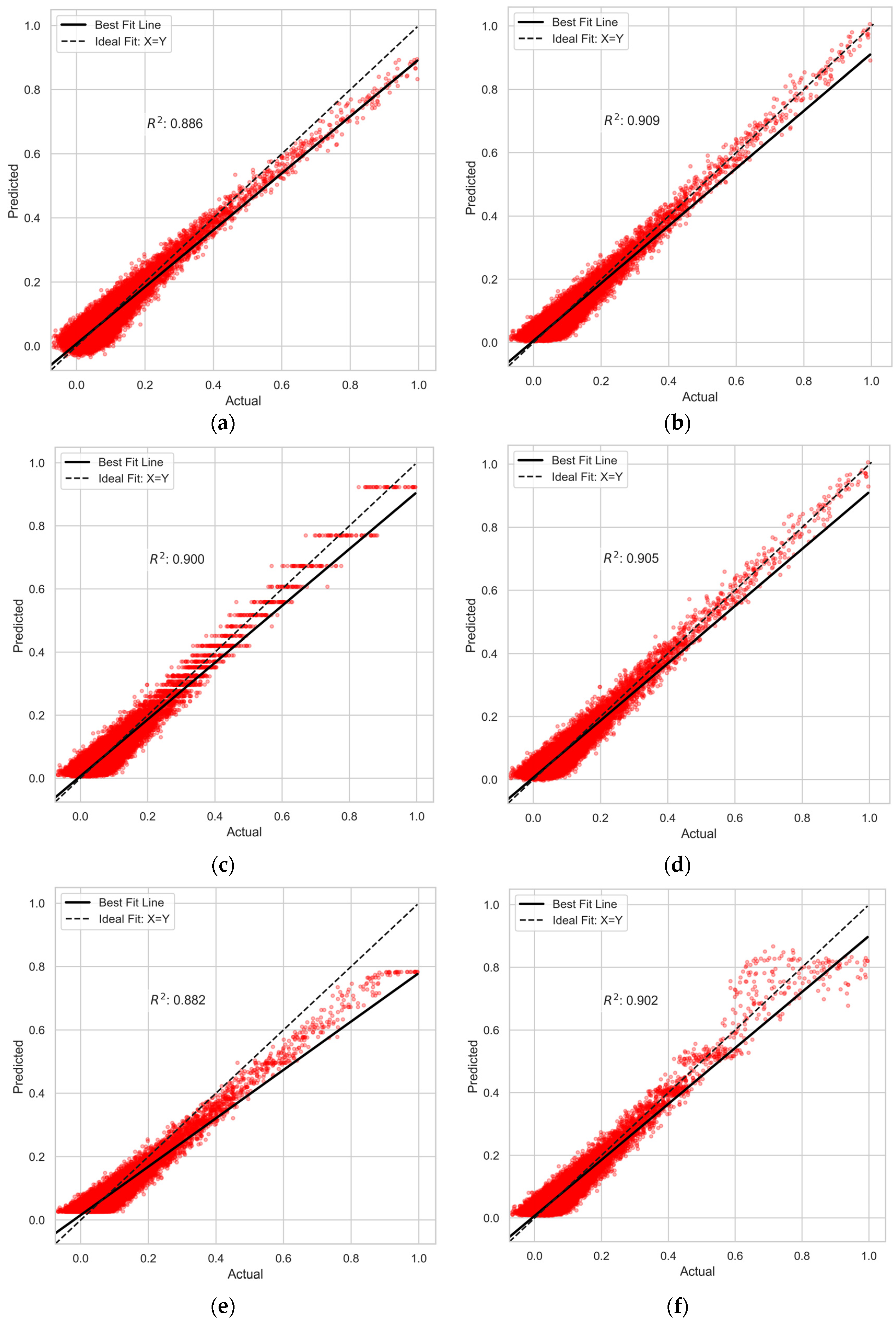
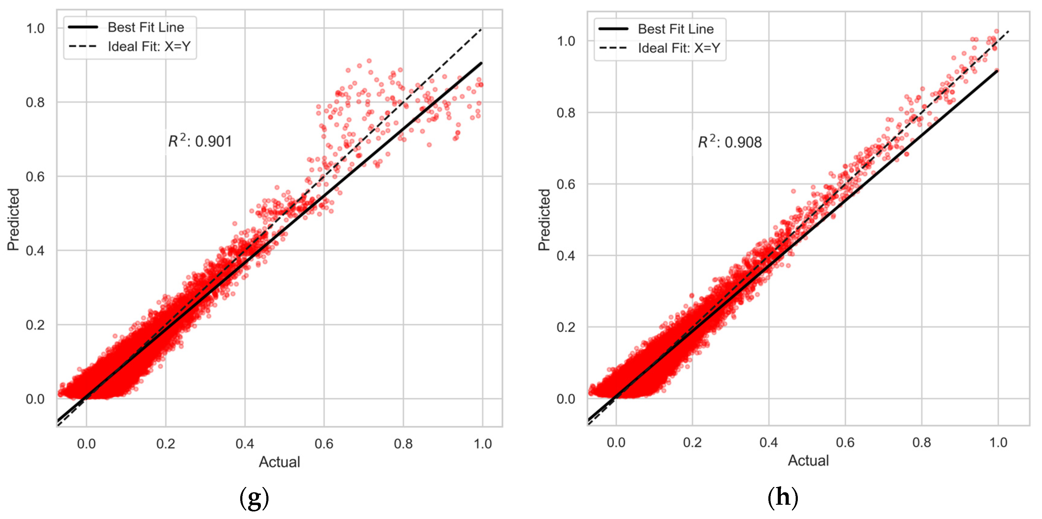
Figure 8 shows the actual versus predicted results for the regression models using testing data. The red dots represent the actual test data values against predicted values as a scatter plot. This plot effectively highlights the models’ generalization abilities outside the training set. The models exhibit similar $R^2$ scores, which suggests that all models effectively captured the underlying data patterns even when exposed to new, unseen data. Notably, the PR model achieved a high $R^2$ score of 0.909, which effectively captures the non-linear relationships between the variables. Similarly, the DNN and RFR models demonstrated excellent fit and predictive precision, with $R^2$ values of 0.906 and 0.905, respectively. Even models with slightly lower but still commendable $R^2$ values, such as LightGBM (0.901) and XGBoost (0.902), demonstrated strong predictive abilities. On the other hand, GB and LR achieved lower $R^2$ scores of 0.882 and 0.886, respectively. Nonetheless, these results validate the capability of both traditional algorithms and advanced machine learning techniques like neural networks to achieve high predictive accuracy and maintain consistency across different data splits.

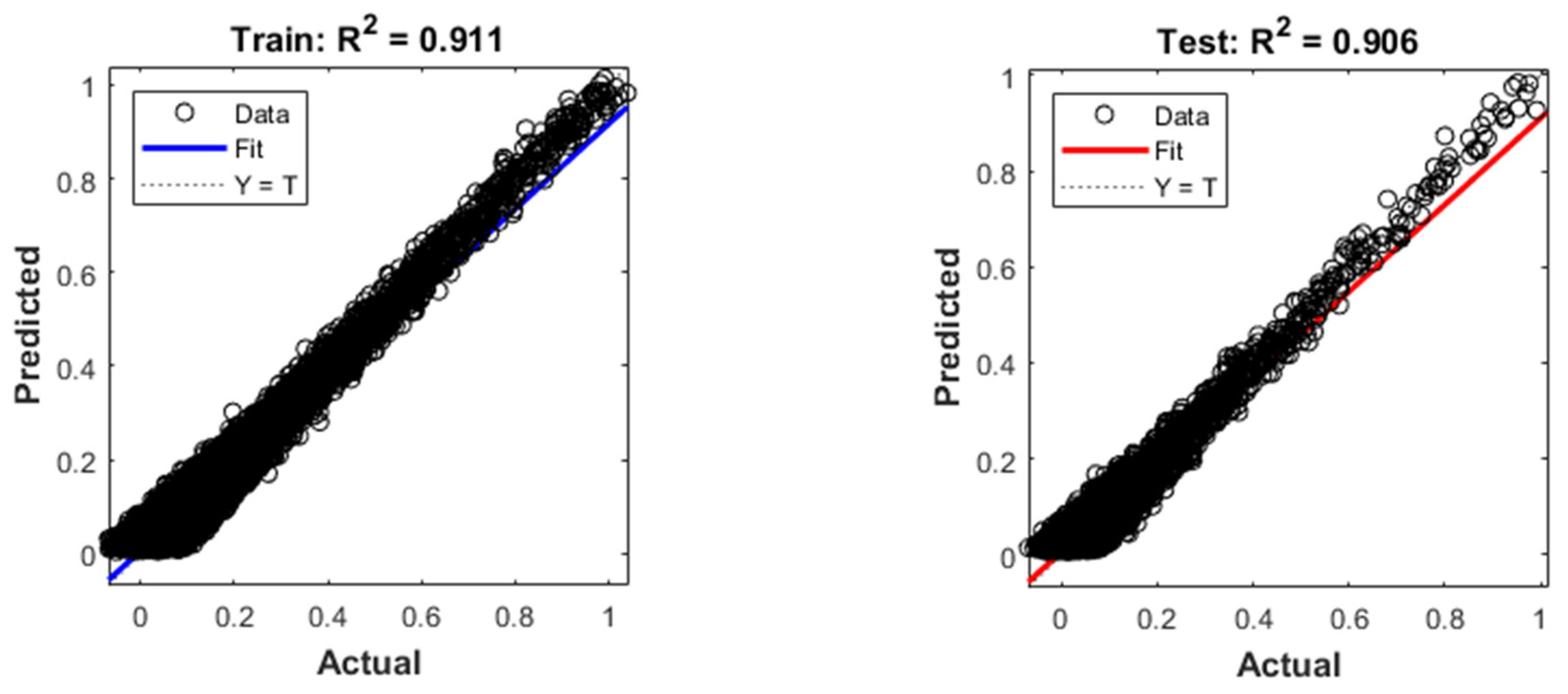
Furthermore, the CFNN model trained using the MATLAB platform captured a high degree of the variability within the training data, with an $R^2$ score of 0.911, whereas it achieved a slightly lower score on the test set, with an $R^2$ of 0.906. The predictive performance of the CFNN across the training and testing set is shown in Figure 9. The closeness of the testing data points to the identity line, and the alignment with the best-fit line demonstrates the model’s effective prediction capability on unseen data.

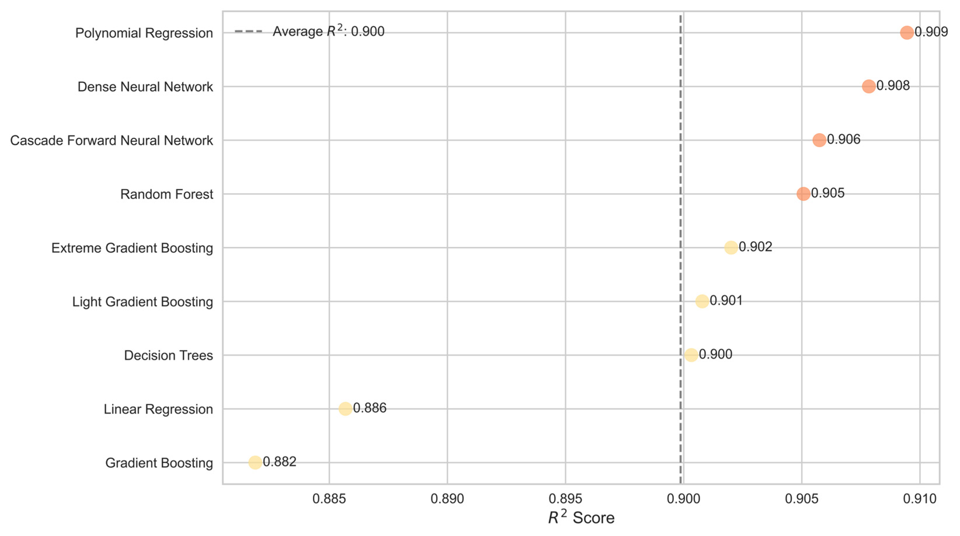
As seen in the dot plot in Figure 10, the performance of all trained models was visually analyzed, with the $R^2$ score on the test set serving as the evaluation metric. The trained models had an average $R^2$ score of 0.9. This means that the models explained 90% of the variance in the test set and demonstrated a strong predictive ability.

Furthermore, in Figure 11, we continue our visual analysis by assessing the performance of the classic machine learning models based on the four metrics used, namely MAE, RMSE, $R^2$, and MAPE.

To ensure accurate representation on the radar chart, it is necessary to normalize the values of the various metrics. Here, 0 signifies the lowest value, while 1 signifies the highest. Typically, a model is deemed effective if it yields low MAE, RMSE, and MAPE scores while achieving high $R^2$ scores on the test data.

The third-degree PR model effectively explained the variance of the data, evidenced by the highest $R^2$ score and the lowest loss errors in the MSE, RMSE, and MAPE metrics. Similarly, RFR maintained a high $R^2$ score while showing minimal losses in MAE, RMSE, and MAPE metrics.

In contrast, DT, XGB, and LGB showed moderate performance, with respectable $R^2$ scores, signifying a decent fit to the data. However, these models struggled with higher error rates in MSE, RMSE, and MAPE metrics, suggesting less consistency in predictions.

On the other hand, GB and LR underperformed relative to other models. Both recorded the lowest $R^2$ scores and also exhibited higher error rates in the MAE, RMSE, and MAPE metrics, further reflecting their limited predictive accuracy and robustness.

Comparing all the models, the superior performance of PR, DNN, and CFNN can be attributed to their ability to capture the non-linear relationships exhibited by many of the features, as illustrated in the pairwise scatter plots in Figure 3 and Figure 4. All three models are well-suited for complex, non-linear interactions, as evidenced by their ability to explain the variability of the data effectively and maintain low error rates. The poor performance of LR can be attributed to its inability to capture non-linear relationships between some of the features.

Therefore, it is necessary to select appropriate machine learning models depending on the existing relationships among the oil reservoir parameters and between these parameters and the oil recovery factor. Comprehensive understanding of the dataset—including its distribution, underlying trends, and potential biases—is critical for training robust machine learning models.

3.2. Permutation Feature Importance Analysis

One of the key advantages of machine learning models is their ability to identify and quantify the importance of different features in making accurate predictions. Permutation importance is one such way of identifying the important features in a model. It works by measuring the change in a model’s performance after permuting (shuffling) the values of a particular feature. The rationale behind the method is that if a feature is important, then shuffling its values should lead to a significant decrease in the model’s performance. The raw permutation values can be normalized to facilitate comparison across different features and models.

Figure 12 illustrates the permutation feature importance across all models. It can be observed that oil and water saturation are the most critical features, with the highest importance across all models, although varying in degree. Polymer concentration holds the third-largest normalized importance score with a relatively consistent impact across all models. In contrast, pressure has moderate relevance, while absolute permeability, porosity, and viscosity show the least importance, meaning that they have a minor impact on model performance overall.

Comprehending the influence of features on decision-making contributes to the explainability of these models, offering insights and transparency into how predictions are made. As a result, it increases trust and confidence in the models’ outputs. Beyond aiding in understanding the models and providing information on how to enhance their performance, knowing the different feature importance helps in prioritizing efforts and resources toward the most impactful factors, resulting in more effective procedures and decision-making. Decision-makers can then optimize oil recovery by adjusting key operational factors, such as injection rates or polymer concentrations, based on these insights.

Additionally, this study demonstrated the robust predictive capabilities of machine learning models on a dataset that is substantially larger and noisier than typically encountered in this research field. The exploration of an extensive dataset and a diverse array of machine learning models provide enhanced predictive capabilities and operational insights that could lead to more effective and economically viable EOR strategies. Further research could explore novel EOR strategies or improve currently used ones. For instance, research can be directed toward finding more economical or efficient ways to leverage important factors, potentially leading to more economical and efficient recovery methods.

4. Conclusions

The results indicate that PR, DNN, and CFNN showed superior performance, with $R^2$ scores of 0.909, 0.908, and 0.906. Moreover, the tree-based models, namely DT, RFR, XGBoost, and LightGB, showed $R^2$ scores between 0.900 and 0.905, indicating good generalization abilities. In contrast, GB and LR performed relatively poor, with $R^2$ scores of 0.882 and 0.886, respectively.

The analysis of the most important features across all models revealed that oil and water saturation were the most significant features to influence the models’ decision-making, whereas viscosity was found to be the least significant feature.

This research demonstrated that machine learning models are capable of effectively capturing patterns from the large-scale synthetic dataset generated using the Buckley–Leverett mathematical model for polymer flooding, even with the introduction of noise. Furthermore, the most effective types of machine learning models for this dataset proved to be a non-linear parametric model (PR) and neural networks (DNN and CFNN).

Despite the results of this research, the use of a synthetic dataset is a limiting factor. Moreover, while this study considered seven key features, numerous other relevant features that could impact model outcomes exist. Future work will involve employing a real-world dataset, incorporating more reservoir parameters, and validating the effectiveness of machine learning models on these more complex and real datasets.

References

1. Wang, C.; Wang, B.; Cao, X.; Li, H. Application and Design of Alkaline-Surfactant-Polymer System to Close Well Spacing Pilot Gudong Oilfield. In Proceedings of the SPE Western Regional Meeting, Long Beach, CA, USA, 25 June 1997. [Google Scholar] [CrossRef]
2. Sheng, J.J.; Leonhardt, B.; Azri, N. Status of Polymer-Flooding Technology. J. Can. Pet. Technol. 2015, 54, 116–126. [Google Scholar] [CrossRef]
3. Zhang, Y.; Wei, M.; Bai, B.; Yang, H.; Kang, W. Survey and Data Analysis of the Pilot and Field Polymer Flooding Projects in China. In Proceedings of the All Days, Tulsa, OK, USA, 11 April 2016; p. SPE-179616-MS. [Google Scholar] [CrossRef]
4. Kamari, A.; Gharagheizi, F.; Shokrollahi, A.; Arabloo, M.; Mohammadi, A.H. Integrating a Robust Model for Predicting Surfactant–Polymer Flooding Performance. J. Pet. Sci. Eng. 2016, 137, 87–96. [Google Scholar] [CrossRef]
5. Sun, Q.; Ertekin, T. The Development of Artificial-Neural-Network-Based Universal Proxies to Study Steam Assisted Gravity Drainage (SAGD) and Cyclic Steam Stimulation (CSS) Processes. In Proceedings of the SPE Western Regional Meeting, Garden Grove, CA, USA, 27–30 April 2015. [Google Scholar] [CrossRef]
6. Amirian, E.; John Chen, Z. Cognitive Data-Driven Proxy Modeling for Performance Forecasting of Waterflooding Process. Glob. J. Technol. Optim. 2017, 8, 1–8. [Google Scholar] [CrossRef]
7. Alade, O.; Al Shehri, D.; Mahmoud, M.; Sasaki, K. Viscosity–Temperature–Pressure Relationship of Extra-Heavy Oil (Bitumen): Empirical Modelling versus Artificial Neural Network (ANN). Energies 2019, 12, 2390. [Google Scholar] [CrossRef]
8. Daribayev, B.; Mukhanbet, A.; Nurakhov, Y.; Imankulov, T. Implementation of The Solution to the Oil Displacement Problem Using Machine Learning Classifiers and Neural Networks. East.-Eur. J. Enterp. Technol. 2021, 5, 55–63. [Google Scholar] [CrossRef]
9. Bansal, Y.; Ertekin, T.; Karpyn, Z.; Ayala, L.; Nejad, A.; Suleen, F.; Balogun, O.; Liebmann, D.; Sun, Q. Forecasting Well Performance in a Discontinuous Tight Oil Reservoir Using Artificial Neural Networks. In Proceedings of the SPE Unconventional Resources Conference/Gas Technology Symposium, The Woodlands, TX, USA, 10 April 2013. [Google Scholar] [CrossRef]
10. Ertekin, T.; Sun, Q. Artificial Neural Network Applications in Reservoir Engineering. In Artificial Neural Networks in Chemical Engineering; NOVA: Hauppauge, NY, USA, 2017; pp. 123–204. [Google Scholar]
11. Karambeigi, M.S.; Zabihi, R.; Hekmat, Z. Neuro-Simulation Modeling of Chemical Flooding. J. Pet. Sci. Eng. 2011, 78, 208–219. [Google Scholar] [CrossRef]
12. Prasanphanich, J. Gas Reserves Estimation by Monte Carlo Simulation and Chemical Flooding Optimization Using Experimental Design and Response Surface Methodology. Ph.D. Thesis, The University of TEXAS at Austin, Austin, TX, USA, 2009. [Google Scholar] [CrossRef]
13. Al-Dousari, M.M.; Garrouch, A.A. An Artificial Neural Network Model for Predicting the Recovery Performance of Surfactant Polymer Floods. J. Pet. Sci. Eng. 2013, 109, 51–62. [Google Scholar] [CrossRef]
14. Alkhatib, A.; Babaei, M.; King, P.R.R. Decision Making Under Uncertainty: Applying the Least-Squares Monte Carlo Method in Surfactant-Flooding Implementation. SPE J. 2013, 18, 721–735. [Google Scholar] [CrossRef]
15. Ahmadi, M.A.; Pournik, M. A Predictive Model of Chemical Flooding for Enhanced Oil Recovery Purposes: Application of Least Square Support Vector Machine. Petroleum 2016, 2, 177–182. [Google Scholar] [CrossRef]
16. Jahani-Keleshteri, Z. A Robust Approach to Predict Distillate Rate through Steam Distillation Process for Oil Recovery. Pet. Sci. Technol. 2017, 35, 419–425. [Google Scholar] [CrossRef]
17. Le Van, S.; Chon, B. Artificial Neural Network Model for Alkali-Surfactant-Polymer Flooding in Viscous Oil Reservoirs: Generation and Application. Energies 2016, 9, 1081. [Google Scholar] [CrossRef]
18. Larestani, A.; Mousavi, S.P.; Hadavimoghaddam, F.; Ostadhassan, M.; Hemmati-Sarapardeh, A. Predicting the Surfactant-Polymer Flooding Performance in Chemical Enhanced Oil Recovery: Cascade Neural Network and Gradient Boosting Decision Tree. Alex. Eng. J. 2022, 61, 7715–7731. [Google Scholar] [CrossRef]
19. Mohammadi, M.-R.; Hemmati-Sarapardeh, A.; Schaffie, M.; Husein, M.M.; Ranjbar, M. Application of Cascade Forward Neural Network and Group Method of Data Handling to Modeling Crude Oil Pyrolysis during Thermal Enhanced Oil Recovery. J. Pet. Sci. Eng. 2021, 205, 108836. [Google Scholar] [CrossRef]
20. Ebaga-Ololo, J.; Chon, B. Prediction of Polymer Flooding Performance with an Artificial Neural Network: A Two-Polymer-Slug Case. Energies 2017, 10, 844. [Google Scholar] [CrossRef]
21. Saboorian-Jooybari, H.; Dejam, M.; Chen, Z. Heavy Oil Polymer Flooding from Laboratory Core Floods to Pilot Tests and Field Applications: Half-Century Studies. J. Pet. Sci. Eng. 2016, 142, 85–100. [Google Scholar] [CrossRef]
22. Alghazal, M. Development and Testing of Artificial Neural Network Based Models for Water Flooding and Polymer Gel Flooding in Naturally Fractured Reservoirs. Master’s Thesis, The Pennsylvania State University, Camp Hill, PA, USA, 2015. [Google Scholar]
23. Norouzi, M.; Panjalizadeh, H.; Rashidi, F.; Mahdiani, M.R. DPR Polymer Gel Treatment in Oil Reservoirs: A Workflow for Treatment Optimization Using Static Proxy Models. J. Pet. Sci. Eng. 2017, 153, 97–110. [Google Scholar] [CrossRef]
24. Amirian, E.; Dejam, M.; Chen, Z. Performance Forecasting for Polymer Flooding in Heavy Oil Reservoirs. Fuel 2018, 216, 83–100. [Google Scholar] [CrossRef]
25. Sun, Q.; Ertekin, T. Screening and Optimization of Polymer Flooding Projects Using Artificial-Neural-Network (ANN) Based Proxies. J. Pet. Sci. Eng. 2020, 185, 106617. [Google Scholar] [CrossRef]
26. Imankulov, T.; Kenzhebek, Y.; Makhmut, E.; Akhmed-Zaki, D. Using Machine Learning Algorithms to Solve Polymer Flooding Problem. In Proceedings of the ECMOR 2022, Hague, The Netherlands, 5–7 September 2022; Volume 2022, pp. 1–9. [Google Scholar] [CrossRef]
27. Makhmut, E.; Imankulov, T.; Daribayev, B.; Akhmed-Zaki, D. Development of Hybrid Parallel Computing Models to Solve Polymer Flooding Problem. In Proceedings of the ECMOR 2022, Hague, The Netherlands, 5–7 September 2022; Volume 2022, pp. 1–14. [Google Scholar] [CrossRef]
28. Saseendran, A.; Setia, L.; Chhabria, V.; Chakraborty, D.; Barman Roy, A. Impact of Noise in Dataset on Machine Learning Algorithms. Mach. Learn. Res. 2019. [Google Scholar] [CrossRef]
29. Kalapanidas, E.; Avouris, N.; Craciun, M.; Neagu, D. Machine Learning Algorithms: A Study on Noise Sensitivity. 2003. Available online: http://delab.csd.auth.gr/bci1/Balkan/356kalapanidas.pdf (accessed on 28 March 2024).
30. James, G.; Witten, D.; Hastie, T.; Tibshirani, R.; Taylor, J. Linear Regression. In An Introduction to Statistical Learning: With Applications in Python; James, G., Witten, D., Hastie, T., Tibshirani, R., Taylor, J., Eds.; Springer International Publishing: Cham, Swizterlands, 2023; pp. 69–134. [Google Scholar] [CrossRef]
31. Lewis, R. An Introduction to Classification and Regression Tree (CART) Analysis. In Proceedings of the Annual Meeting of the Society for Academic Emergency Medicine, San Francisco, CA, USA, 22–25 May 2000. [Google Scholar]
32. Breiman, L. Random Forests. Mach. Learn. 2001, 45, 5–32. [Google Scholar] [CrossRef]
33. Friedman, J.H. Greedy Function Approximation: A Gradient Boosting Machine. Ann. Stat. 2001, 29, 1189–1232. [Google Scholar] [CrossRef]
34. Chen, T.; Guestrin, C. XGBoost: A Scalable Tree Boosting System. In Proceedings of the 22nd ACM SIGKDD International Conference on Knowledge Discovery and Data Mining, San Francisco, CA, USA, 13–17 August 2016; pp. 785–794. [Google Scholar]
35. Ke, G.; Meng, Q.; Finley, T.; Wang, T.; Chen, W.; Ma, W.; Ye, Q.; Liu, T.-Y. LightGBM: A Highly Efficient Gradient Boosting Decision Tree. In Proceedings of the 31st International Conference on Neural Information Processing Systems, Long Beach, NY, USA, 4–9 December 2017; pp. 3149–3157. [Google Scholar]
36. Goodfellow, I.; Bengio, Y.; Courville, A. Deep Learning; The MIT Press: Cambridge, MA, USA, 2016; pp. 164–223. [Google Scholar]
37. Nair, V.; Hinton, G.E. Rectified Linear Units Improve Restricted Boltzmann Machines. In Proceedings of the 27th International Conference on International Conference on Machine Learning, Haifa, Israel, 21–24 June 2010; pp. 807–814. [Google Scholar]
38. Warsito, B.; Santoso, R.; Suparti; Yasin, H. Cascade Forward Neural Network for Time Series Prediction. J. Phys. Conf. Ser. 2018, 1025, 012097. [Google Scholar] [CrossRef]
39. Hodson, T.O. Root-Mean-Square Error (RMSE) or Mean Absolute Error (MAE): When to Use Them or Not. Geosci. Model Dev. 2022, 15, 5481–5487. [Google Scholar] [CrossRef]
Figure 1. Correlation matrix of the reservoir parameters and oil recovery factor.
Energies 17 03397 g001
Figure 2. Pairwise scatter plots of the following selected variables: (a) Pressure vs. recovery factor. (b) Pressure vs. polymer concentration. (c) Polymer concentration vs. oil saturation. (d) Pressure vs. oil saturation. (e) Pressure vs. porosity. (f) Water saturation vs. oil saturation. (g) Oil saturation vs. polymer concentration. (h) Oil saturation vs. recovery factor. (i) Water saturation vs. recovery factory. (j) Water saturation vs. polymer concentration. (k) Water saturation vs. pressure. (l) Polymer concentration vs. recovery factor.
Energies 17 03397 g002
Figure 3. Correlation matrix of the reservoir parameters and oil recovery factor after adding Gaussian noise.
Energies 17 03397 g003
Figure 4. Pairwise scatter plots of the following variables after adding Gaussian noise: (a) Pressure vs. recovery factor. (b) Pressure vs. polymer concentration. (c) Polymer concentration vs. oil saturation. (d) Pressure vs. oil saturation. (e) Pressure vs. porosity. (f) Water saturation vs. oil saturation. (g) Oil saturation vs. polymer concentration. (h) Oil saturation vs. recovery factor. (i) Water saturation vs. recovery factory. (j) Water saturation vs. polymer concentration. (k) Water saturation vs. pressure. (l) Polymer concentration vs. recovery factor.
Energies 17 03397 g004
Figure 5. DNN architecture for predicting recovery factors from the reservoir parameters.
Energies 17 03397 g005
Figure 6. CFNN architecture for predicting recovery factor from the reservoir parameters.
Energies 17 03397 g006
Figure 7. Comparison of predicted versus actual values on the training set for (a) linear regression, (b) polynomial regression, (c) decision tree, (d) random forest, (e) gradient boosting, (f) extreme gradient boosting, (g) light gradient boosting, and (h) dense neural networks.
Energies 17 03397 g007aEnergies 17 03397 g007b
Figure 8. Comparison of predicted versus actual values on the test set for (a) linear regression, (b) polynomial regression, (c) decision tree, (d) random forest, (e) gradient boosting, (f) extreme gradient boosting, (g) light gradient boosting, and (h) dense neural networks.
Energies 17 03397 g008aEnergies 17 03397 g008b
Figure 9. Comparison of predicted versus actual values on the testing set for the CFNN model.
Energies 17 03397 g009
Figure 10. Comparison of R 2 scores across all trained models.
Energies 17 03397 g010
Figure 11. Multi-metric performance evaluation of classic machine learning models.
Energies 17 03397 g011
Figure 12. Permutation importance of features across all machine learning models trained.
Energies 17 03397 g012