Long Short-Term Renewable Energy Sources Prediction for Grid-Management Systems Based on Stacking Ensemble Model

Abstract

The transition towards sustainable energy systems necessitates effective management of renewable energy sources alongside conventional grid infrastructure. This paper presents a comprehensive approach to optimizing grid management by integrating Photovoltaic (PV), wind, and grid energies to minimize costs and enhance sustainability. A key focus lies in developing an accurate scheduling algorithm utilizing Mixed Integer Programming (MIP), enabling dynamic allocation of energy resources to meet demand while minimizing reliance on cost-intensive grid energy. An ensemble learning technique, specifically a stacking algorithm, is employed to construct a robust forecasting pipeline for PV and wind energy generation. The forecasting model achieves remarkable accuracy with a Root Mean Squared Error (RMSE) of less than 0.1 for short-term (15 min and one day ahead) and long-term (one week and one month ahead) predictions. By combining optimization and forecasting methodologies, this research contributes to advancing grid management systems capable of harnessing renewable energy sources efficiently, thus facilitating cost savings and fostering sustainability in the energy sector.

1. Introduction

Global efforts to convert to renewable energy sources are being propelled by worries about sustainability, energy security, and climate change. Photovoltaic (PV) and wind energy technologies have become major players in this space, with promising futures for environmentally friendly power production. Nevertheless, to make the most of these resources, it is necessary to maximize their integration into the current energy infrastructure using advanced scheduling algorithms and predictive models.

This work is driven by the necessity to improve the effectiveness and dependability of renewable energy systems, specifically those utilizing PV and wind power. Although previous work has made significant progress, there are still difficulties in precisely forecasting the production of renewable energy sources over different time periods and efficiently integrating them into the electricity grid. The current body of research has predominantly concentrated on developing models for short-term predictions (next 15 min and day ahead) [1,2,3,4,5], resulting in a lack of accurate long-term projections (one week and one month) [6,7,8,9]. In addition, conventional scheduling algorithms frequently overlook the unpredictability and intermittency that are inherent in the generation of solar and wind energy.

Related studies on scheduling algorithms for integrating renewable energy sources, particularly PV and wind, underscore the necessity of accurate prediction methods for long-term forecasting. Despite considerable progress, challenges persist in forecasting energy generation for longer horizons, such as one day, one week, and one month ahead. Existing methods struggle with complexities like seasonal variations, weather dynamics, and environmental factors, limiting their accuracy over extended periods. This can lead to sub-optimal scheduling decisions, increased reliance on grid energy, and potential imbalances in supply and demand. Enhancing the accuracy of long-term forecasts is crucial for improving resource allocation, energy storage, and demand management in grid systems, ultimately enhancing efficiency and sustainability.

Our research aims to tackle these challenges through the pursuit of two fundamental objectives:

1.

Our primary focus tackles the crucial need for developing independent or hybrid forecasting models specifically for PV and wind energy prediction. Reliable forecasts enable grid operators to integrate these PV and Wind energy effectively, minimizing the need for costly backup power generation. Additionally, accurate forecasts support efficient energy market operations, inform policymakers about optimal resource allocation, enhance grid stability, and contribute to cost reduction in energy production and distribution.

2.

Our second interest relies on developing cost-effective solutions for scheduling the utilization of PV, wind, and grid energies. This study acknowledges the complex relationship between predictions, power costs, and environmental elements in maximizing energy efficiency. An analysis of several solutions entails a comprehensive approach, taking into account real-time energy expenses, grid requirements, and weather predictions. Developing an adaptive scheduling pipeline that aims to optimize cost savings, decrease the carbon footprint, and emphasize the system’s capacity to react dynamically to different grid situations.

The approach we adopt in this work is illustrated in Figure 1.

This paper consists of 4 sections and is organized systematically to thoroughly examine predictive modeling and scheduling algorithms for renewable energy systems. Section 2 reviews the most common RE forecasting models. Section 3 provides a detailed examination of PV power, including an exploration of their operating principles, determinants of energy production, and current methodologies for forecasting. Section 4 is dedicated to the Wind power dataset analysis and prediction. Section 5 presents a thorough examination of the scheduling pipeline based on the Mixed Integer Programming (MIP) technique. Section 6 concludes the paper and describes future work.

2. Renewable Energies (RE) Forecasting Models

2.1. Forecasting Model

2.1.1. Time Series Models

The initial exploration of time series forecasting for RE production considered autoregressive models and moving averages like the Weighted Moving Averages (WMA) and the AutoRegressive Integrated Moving Average (ARIMA).

• Weighted Moving Averages (WMA): The decision to implement the WMA model for RE forecasting was made based on its suitability for capturing short-term fluctuations and its simplicity. However, it became evident that the model struggled to generalize effectively for the broader range of predictions required. While WMA excels at emphasizing recent data points, its simplistic approach may not adequately capture underlying trends or structural shifts in the data, particularly over longer timeframes. Consequently, the model’s limitations in generalization compromised its ability to provide accurate forecasts beyond short-term horizons, highlighting the need for alternative or supplementary forecasting algorithms that can better address the complexities of PV energy production patterns across various timescales [10].
• AutoRegressive Integrated Moving Average (ARIMA): ARIMA is a powerful technique for forecasting time series data. It combines autoregression, differencing, and moving averages seamlessly. The main advantage of this is its ability to effectively capture both immediate changes and long-term patterns in renewable energy data. The application of ARIMA involves a rigorous procedure of determining the most suitable order of differencing, autoregressive components, and moving average components through comprehensive statistical analysis [11].

The cited models can capture sequential dependencies and seasonal variations, however, they faced limitations in handling the intricate and dynamic nature of RE production patterns.

2.1.2. Machine Learning (ML) Models

A wide range of machine learning algorithms, including Gradient Boosting Regressor [12], K-Neighbors Regressor [13], Random Forest [14], Linear Regression, LightGBM, XGBoost [15], SVR, AdaBoost Regressor [16], Bagging Regressor, and XGB Regressor, as well as other models, were used to improve predictive accuracy over various time horizons. When delving into the specifics of each model, LightGBM’s implementation stands out for its strategic use of gradient boosting approaches, which leverage efficient algorithms and rigorous hyperparameter adjustment to enhance accuracy while minimizing overfitting. Support Vector Regression (SVR) takes a unique technique, managing nonlinear relationships using the kernel trick and exhibiting robustness to outliers using epsilon-insensitive loss functions. Meanwhile, the Gradient Boosting Regressor (GBR) demonstrates the power of ensemble learning by gradually refining weak learners to properly capture complicated data correlations. Finally, XGBRegressor appears as a strong candidate for RE forecasting, utilizing its ability to capture non-linear patterns and efficiently manage missing data, hence improving predictive performance for RE generation. These solutions demonstrate a multidimensional approach to predictive modeling, which combines accuracy, efficiency, and adaptability to negotiate the intricacies of various datasets and forecasting jobs.

2.1.3. Deep Learning (DL) Algorithms

To capture non-linear interactions in the data, DL techniques such as MLP Regressor, RNN, CNN, and LSTM were investigated for RE production forecasting. Getting into the intricacies of each DL method, the use of MLP Regressor offers an important avenue in renewable energy research, providing a versatile framework for modeling complicated interactions within sequential data. RNNs, which are ideally adapted to modeling sequential data, can capture temporal dependencies within RE generation patterns, allowing for more accurate predictions. CNNs have been adapted to capture underlying temporal patterns in RE generation. They excel at recognizing complicated relationships among sequential data, which is critical for efficient grid management. Furthermore, integrating LSTM neural networks into a TensorFlow-Keras framework improves forecasting accuracy by capturing the deep temporal correlations and sequential patterns found in RE data. However, tackling the complexities and uncertainties involved with RE forecasting may necessitate additional techniques beyond LSTM integration, like as ensemble methods or feature engineering, to improve forecasting precision.

2.1.4. Stacking Algorithm

The limitations of individual models are recognized, and, therefore, introduced an ensemble learning technique called stacking. The objective was to consolidate the strengths of different algorithms into a single forecasting model that could handle challenges related to various forecasting horizons [17].

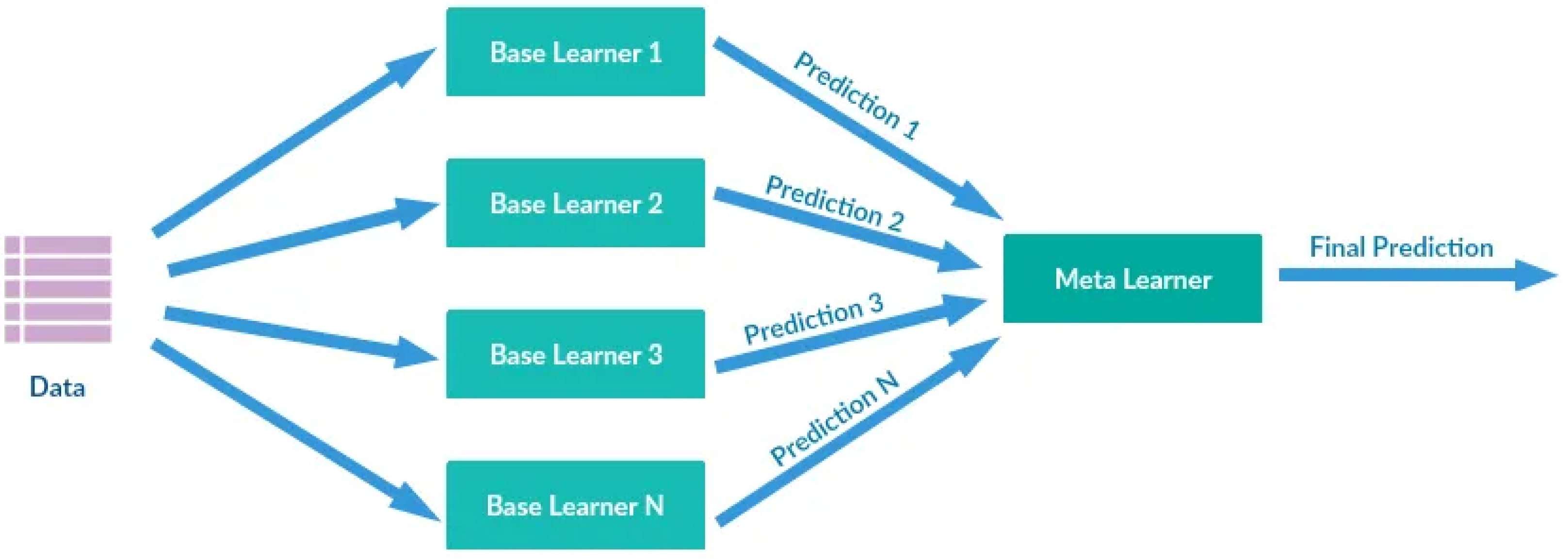
Ensemble learning, specifically stacking model presents users with a solution for limiting aspects of single models by integrating their prediction powers together. This approach is designed to exploit the differences in algorithmic results so that they can be combined to form a strong forecasting framework capable of addressing various foresight windows.

Stacking model, whose architecture is shown in Figure 2, is made up of three main components: (i) the dataset to be stacked upon, (ii) many base learner models, (iii) and ultimately a metalearner which orchestrates the final prediction [18]. Stacking stitches together knowledge from different models thus improving the predictive accuracy while it also prevents overfitting. Furthermore, its ability to adapt to various data distributions and problem complexities makes stacking a versatile approach across different domains. Therefore, ensemble learning represented by stacking model demonstrates that cooperation is one of the effective ways in which prediction analytics can be done.

3. PV Power Forecasting

We have built our research on a foundation of a thorough examination of two essential datasets; the PV dataset and the weather dataset in our quest to improve RE sources.

3.1. PV Dataset

3.1.1. Description

The PV dataset, showcasing historical solar energy production, serves as a foundational resource for developing advanced prediction models by unveiling trends and fluctuations, crucial for PV system research and forecasting. The data is collected in Bavaria, Germany and is provided in Excel format. It is captured at 15-min intervals and covers the time period from 1 May 2016 to 2 August 2022, showing how the PV system has changed over history. The measured value (‘Power’) and its accompanying status are displayed alongside each timestamped entry in the collection.

3.1.2. PV Dataset Features

The dataset is meticulously organized, with three crucial features:

1.

Timestamp: This feature is dedicated to displaying the exact date and time of each recorded data point in the collection.

2.

Power: This critical feature captures the measured values of the PV system, which is the major variable of importance in our analysis. The ‘Power’ entries use a quantitative approach, representing the quantitative components of energy generation and providing insights into the system’s performance.

3.

Status: The ‘Status’ column indicates the operational status of the PV system at each date. This category data enables a thorough understanding of the system’s operation across time, assisting in the detection of patterns and abnormalities that may impact energy generation.

3.2. Meteorological Dataset

3.2.1. Description

The dataset under discussion is a comprehensive compilation of meteorological and solar radiation measurements taken at hourly intervals. This comprehensive dataset, which runs from 1 January 2016 to 27 December 2022, provides thorough insights into air conditions and solar radiation exposure during that time period. The meteorological dataset was obtained through web scraping from the “Deutscher Wetterdienst” website https://www.dwd.de (accessed on 10 November 2023).

3.2.2. Meteorological Features

• Sky Coverage and Precipitation: The sky coverage degree percent indicates cloud cover, while precipitation quantity in millimeters informs about rainfall.
• Solar Radiation and Sunshine Duration: The sum of radiation measurements (atmospheric, diffuse, and global) provides cumulative data on different types of radiation. Meanwhile, the sum of sunshine minutes quantifies the duration of sunshine in 15-min intervals, offering insights into sunlight patterns. Additionally, the sun angle indicates solar exposure by describing the angle of the sun.
• Temperature and Humidity: The temperature air degree Celsius measures air temperature, crucial for assessing PV system performance. Meanwhile, humidity percent indicates the level of humidity, affecting overall atmospheric conditions.
• Wind Information: Wind speed, measured at 15-min intervals, provides crucial data for analyzing environmental conditions. Additionally, wind direction indicates the origin of the wind flow, offering insights into atmospheric dynamics.

3.2.3. Dataset Integration Strategy

To enhance the collaboration between the weather and PV datasets, a thorough modification was undertaken to synchronize their temporal structures. In contrast to the PV dataset, which maintains a 15-min timestamp interval, the weather dataset updates every hour. To address the discrepancy, the time period of the meteorological dataset was adjusted from one hour to fifteen minutes. By performing this operation, which entails duplicating each row with unique timestamps, the two datasets are seamlessly merged.

3.2.4. Preprocessing Strategies for the Integrated PV and Weather Dataset

Different steps were adopted to improve the temporal granularity, feature engineering, and overall data refinement of the PV dataset. The discrete steps taken are summarized as follows:

• Date/time Transformation: The Date column is transformed regarding a standardized date/time format to ensure the establishment of a consistent temporal framework adapted to time series analysis.
• Temporal Feature Extraction: Extracting temporal components from the Date column, such as the day of the week, month, and hour of measurement, allows for a more sophisticated understanding of energy trends across time dimensions.
• Introduction of Interaction Terms: The generation of interaction terms, as illustrated by ‘Interaction1’ which signifies the product of ‘QUANTITY_IN_MM’ and ‘TEMPERATURE_AIR_DEGREE_CELSIUS’, is intended to document interdependent relationships that exist within the dataset.
• Domain-Informed Feature Engineering: Domain-specific knowledge informs the development of supplementary attributes, such as the binary ‘Raining_Category’, and the square of TEMPERATURE_AIR_DEGREE_CELSIUS’ which contribute to a more intricate depiction of environmental conditions.
• Temporal Lag Features and Rolling Mean: By including latency features (‘Power_i’) and a rolling mean of the ‘Power’ variable, the temporal context of the dataset is expanded, enabling the capture of historical patterns and trends.
• Handling Missing Values: To ensure data integrity, rigorous steps are implemented to address missing values caused by the introduction of lag characteristics. This is achieved by carefully removing the related rows.

The resulting dataset, which has been improved in terms of time-related characteristics and enhanced variables, is now ready for advanced modeling and forecasting in the wider field of renewable energy research.

3.3. Exploratory Data Analysis (EDA)

3.3.1. Base Description and Descriptive Statistics

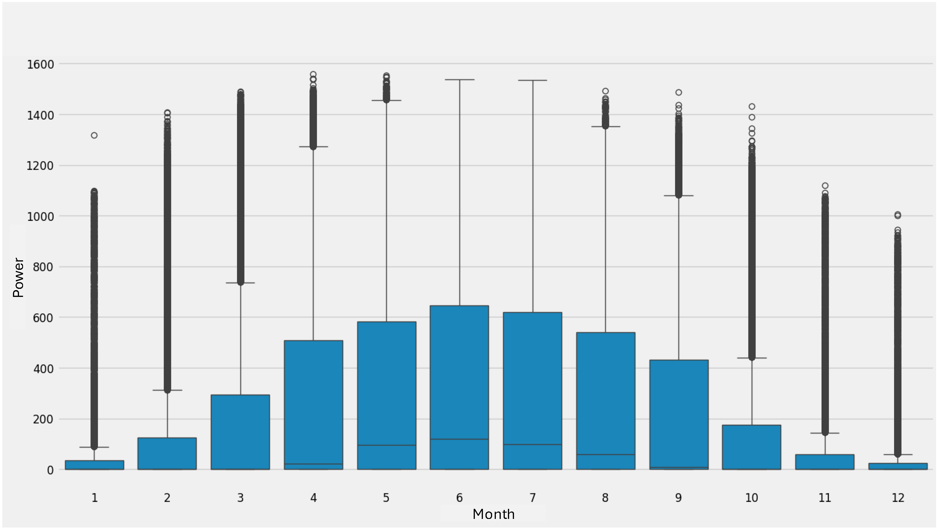
Figure 3 depicts the distribution of the produced PV Power across months. The central line in the box indicates the median, which means that half of the Power in kWh measured in a particular month was less than 200 kWh and the other half was greater. The box’s lower and upper borders represent the first Quartile (Q1) and the third Quartile (Q3), indicating that 25% and 75% of the measured warts were smaller than Q1 and Q3, respectively. The whiskers extending from the box suggest a range of 1.5 times the InterQuartile Range (IQR) above Q3 and below Q1. Any data points that exceed these whiskers are considered outliers. In the boxplot, the concentration of warts is largest between months 6 and 10, with the median wart size exceeding that of the other months. Notably, no outliers are present.

3.3.2. Stationary Test

Two hypothesis tests were conducted using the Dickey-Fuller Test to analyze the characteristics of the Integrated dataset further.

The first test involved doing a two-tailed hypothesis test to evaluate whether the mean of the dataset differed significantly from a predetermined value. By employing a standard significance level ($\alpha$) of 0.05, we tested the null hypothesis (H0: $\mu ={\mu }_0$) with the alternative hypothesis (H1: $\mu \ne {\mu }_0$), where $\mu$ represents the mean value of the population and ${\mu }_0$ is the predetermined value. A chi-square goodness-of-fit test was performed as the second test to examine the distribution of categorical variables in the dataset. The null hypothesis (H0) posits that the observed distribution conforms to the expected distribution when appropriate categories are chosen and the distribution is predicted. The hypothesis tests were performed using standard statistical procedures, which involved the utilization of suitable test statistics and critical values. The experiments yielded valuable information regarding both the average and distributional characteristics of the Integrated dataset. By conducting a comprehensive analysis that incorporates the Dickey-Fuller Test together with other hypothesis tests, we enhance our understanding of the characteristics of the dataset and gain valuable insights for future analytical approaches.

3.3.3. PV Dataset Decomposition

Figure 4 offers a thorough analysis of the PV dataset, dividing it into three key components: trend, seasonality, and residuals. The trend component, which represents the long-term movement in the data, shows a clear upward trajectory, indicating a general positive tendency over the observed time period. Simultaneously, the seasonality component reveals recurring patterns with high and low points happening annually. The repetitive pattern seen indicates the existence of regular seasonal effects, which external causes like weather conditions or holiday seasons could cause. The residuals component, which represents the unexplained variance in the time series after considering trend and seasonality, seems to display random swings around zero. This observation indicates that there is a minimal amount of noise or unusual data points in the dataset, which further supports the reliability and strength of the decomposition model. In summary, this interpretation improves our comprehension of the fundamental patterns inside the PV dataset, offering useful insights for educated analysis and prediction.

3.4. Data Partitioning and Model Evaluation Strategy

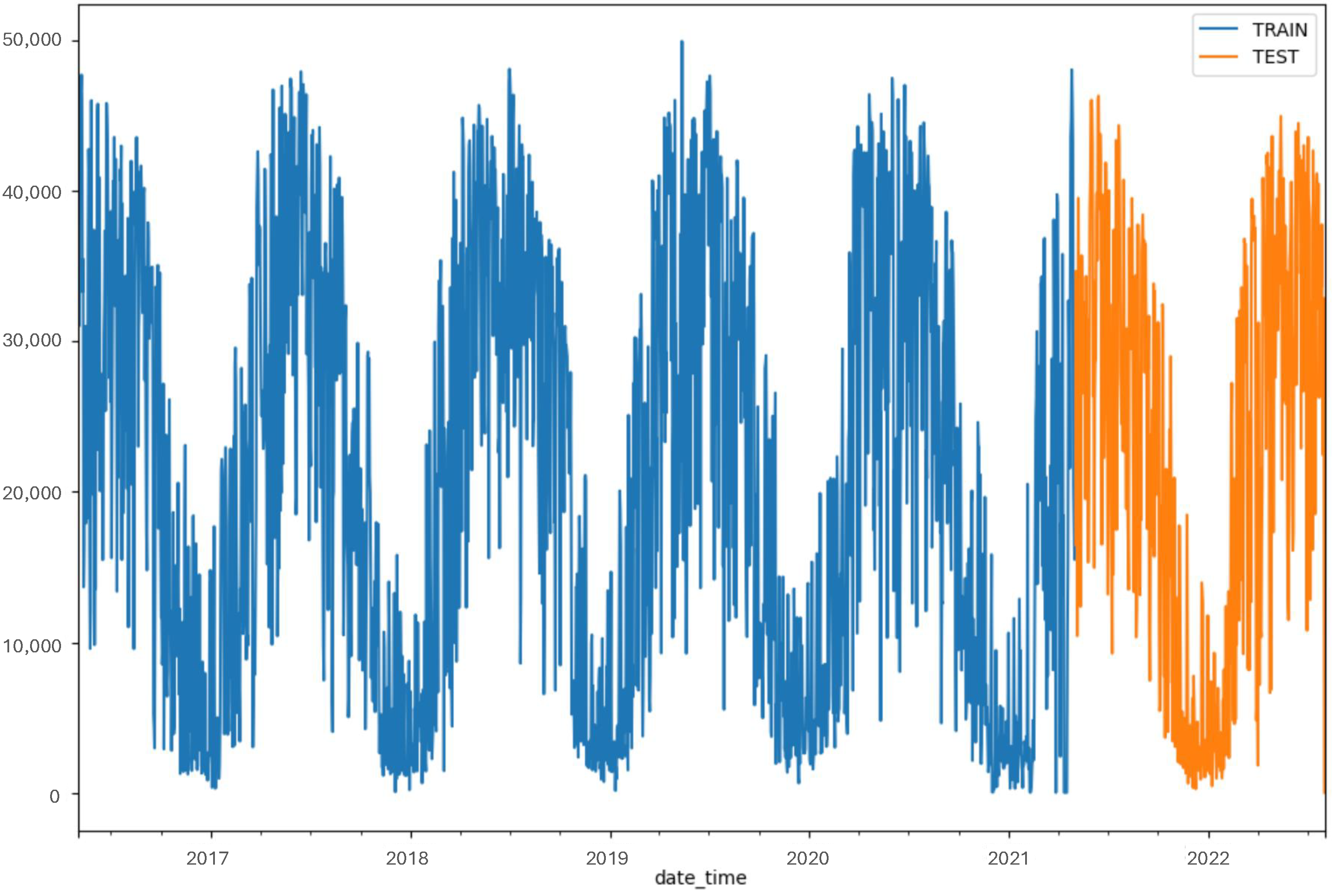
To ensure an impartial evaluation of our PV forecasting model, we have implemented a data-splitting methodology. Figure 5 shows that the dataset has been partitioned into a training set, including 80% of the data, and a test set, encompassing the remaining 20%. This split facilitates model training on the training set while reserving a portion for evaluating the model’s capacity to generalize. Through the implementation of this technique, our goal is to reduce overfitting and provide a dependable evaluation of the model’s predictive performance in real-world situations.

When attempting to ascertain the optimal forecasting model, selecting the appropriate hyperparameters is of utmost importance. To address this problem, we incorporate k-fold cross-validation into the model training procedure. To be more specific, the training set is divided into k subsets, and the model is trained on k-1 folds, while the remaining fold is utilized for validation. The operation is iterated k times, ensuring that each fold is utilized as the validation set exactly once. In each iteration of the cross-validation procedure, the model is trained on k-1 folds and subsequently validated on the remaining fold. The average performance across all folds is then used to evaluate the model’s ability to withstand and generalize. During each iteration of the cross-validation procedure, a grid search is conducted to identify the most efficient combination of hyperparameters. This rigorous examination involves assessing several hyperparameter values, such as learning rates, regularization terms, or model topologies. The hyperparameters that yield the highest validation performance are selected as the ideal combination. The forecasting model is thoroughly trained using the entire training set, employing the optimal hyperparameters determined through cross-validation. The training procedure involves repeatedly modifying the model parameters to minimize the selected loss function. Subsequently, the model’s performance is comprehensively assessed on the specified test set, providing an unbiased assessment of its predictive accuracy in real-world scenarios. To evaluate the efficacy of the forecasting model, we employ the standard evaluation criterion Root Mean Squared Error (RMSE).

3.5. Forecasting Models

3.5.1. Single Model

We have opted for the following forecasting model to predict the PV data: Autoregressive Models, Weighted Moving Averages, Simple Exponential Smoothing, Holt-Winters, ARMA, ARIMA, Gradient Boosting, Random Forest, AdaBoost, K-Neighbors, SVM, XGBoost, Bagging, Extra Trees, MLP Neural Network, MLP Neural Network, RNN, LSTM, CNN and GRU.

3.5.2. Stacking Model Architecture

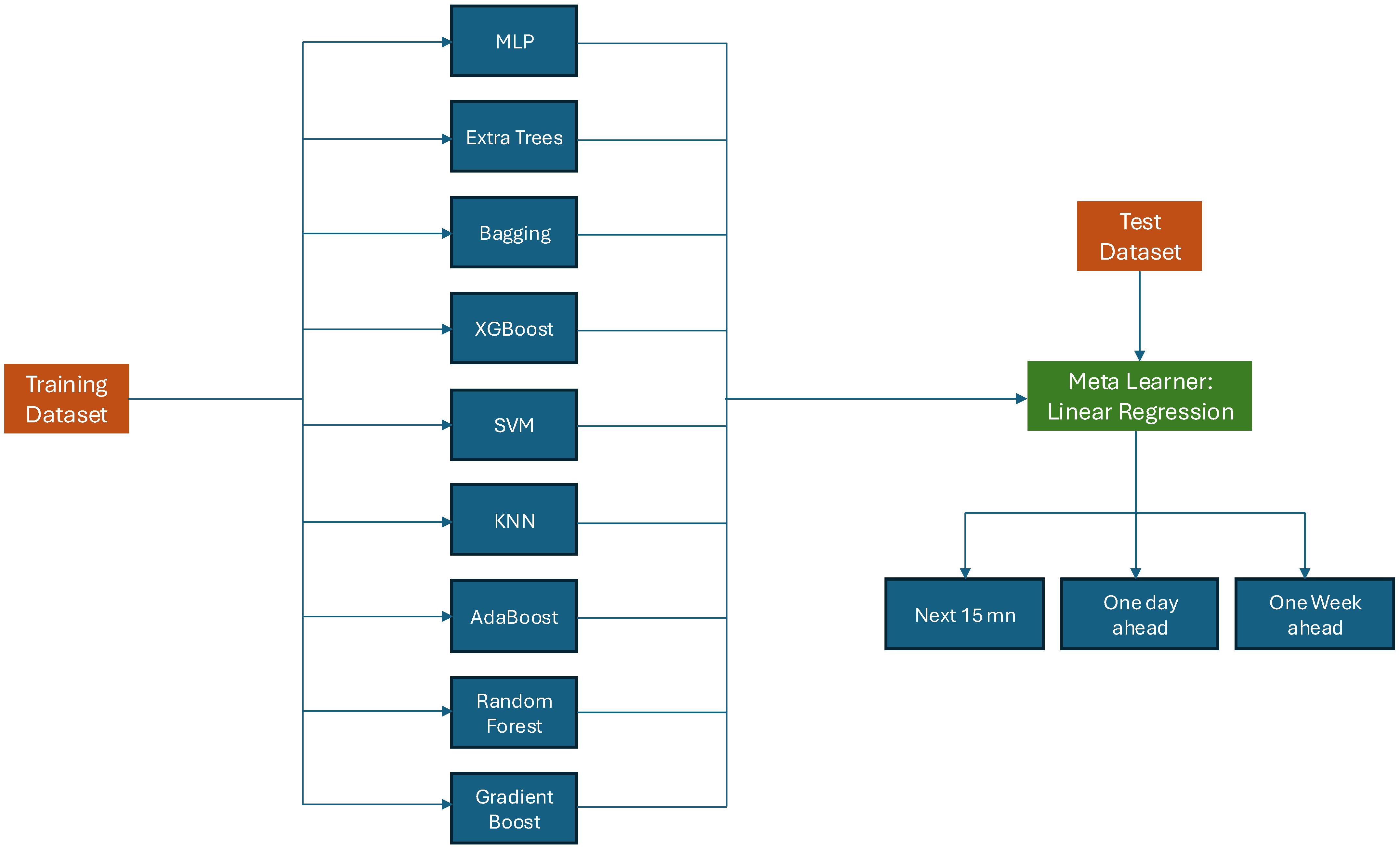
The architecture of the adopted stacking model is shown in Figure 6 and contains the following components:

• Base Models: For the base models, we have used different regression capabilities. For instance, in this example, some of the models are Gradient Boosting, Random Forest, AdaBoost, Linear Regression, K-Neighbors, SVM, XGBoost, Bagging, Extra Trees MLP Neural Network and optionally others.
• StackingRegressor: The models are then brought together in a single ensemble model, which is StackingRegressor. Every base model becomes a learner contributing to the prediction at the overall level.
• Final Estimator (Linear Regression in this case): A linear regression final estimator or something simple is most suitable for combining model predictions. This last estimator fine-tunes and improves forecasts made by many basic models.
• Training and Prediction: The training dataset is used for training the StackingRegressor (X_train and y_train). Both train and test datasets are predicated upon.
• Evaluation: To evaluate the performance of our algorithm on both train and test datasets we calculate RMSE as well as MAPE for StackingRegressor.

For training the models, we used the following hardware specifications:

• GPU: NVIDIA Tesla V100.
• CPU: Intel Xeon E5-2698 v4.

3.6. Results

One Single Forecasting Model

Table 1. PV Comparison of RMSE for Different Forecasting Models.

Model	RMSE Next 15 min	RMSE One Day Ahead	RMSE One Week Ahead	RMSE One Month Ahead
Autoregressive Models	15.2	25.7	90.2	200.5
Weighted Moving Averages	12.3	21.3	70.4	180.2
Simple Exponential Smoothing	18.4	27.3	120.6	230.9
Holt-Winters	22.1	28.9	95.4	210.3
ARMA	20.2	32.5	140.6	250.1
ARIMA	17.6	23.6	103.1	220.8
Gradient Boosting	12.4	19.5	78.6	190.7
Random Forest	9.4	17.3	54.6	160.4
AdaBoost	8.3	18.3	56.4	165.2
K-Neighbors	16.2	34.5	76.9	200.9
SVM	11.7	26.3	56.8	175.6
XGBoost	9.6	17.7	48.8	150.3
Bagging	10.5	28.6	55.2	170.1
Extra Trees	13.8	25.3	78.2	205.8
MLP Neural Network	14.7	23.5	69.4	195.6
RNN	11.3	20.8	62.6	185.4
LSTM	13.2	23.5	39.6	160.2
CNN	9.4	24.9	70	175.8
GRU	9.7	18.5	58.2	170.6
Stacking Model	0.000001	0.0000287	0.0000492	0.000331

represents the RMSE values under different time horizons, i.e., the next 15 min, one day ahead, one week ahead and next month, across diverse prediction models.

• Next 15 min Prediction: The complete assessment of different predictive models has been done in the Next 15 min Prediction task and the results show informative performance measures. Significantly, AdaBoost Models are among the best predictors with a minimum RMSE of 8.3 which shows their efficiency in capturing and utilizing intricate patterns in dataset. The latter comes out as being particularly strong within this predictive environment, implying that they are good at capturing temporal dependencies and using historical information for accurate forecasting. Otherwise, RNN, Random Forest and XGBoost models give a comparable outcome but it fails to beat AdaBoost Model. Therefore, this study not only provides insights into predictions but also offers useful suggestions for the improvement of other similar future prediction cases.
• One Day Ahead Prediction: Various models were carefully examined for one day ahead forecast and among them, GRU model proved to be the best. The GRU model is reported to have the lowest RMSE value of 18.5 when compared to other models. This suggests that it captures very well short-term temporal dependencies and patterns embedded in the data thereby increasing its forecasting ability for one day ahead. It is important to note that over this time frame, the GRU model performs better than Gradient Boosting and XGBoost among others. This simply means that with regard to how intricately it can put together such information from all sources at its disposal, few models can compete with GRU’s predictive abilities.
• One Week Ahead Prediction: Various models’ evaluation of their performance in the context of one-week ahead predictions show that the LSTM model is the most accurate as manifested by its least RMSE among those considered. Specifically, the LSTM model records an impressive RMSE value of 39.6.
• One Month Ahead Prediction: When considering forecasts made one month ahead, it can be seen that the LSTM model had the lowest RMSE of all other models reviewed showing its accuracy at that time period. The LSTM model achieved a further low value of RMSE equal to 160.2 which underlines more its exactitude.

3.7. Stacking Model Prediction

Table 1 shows how Stacking Model has changed the forecast environment and attained unprecedented accuracy with 0% RMSE for all horizons; next 15 min, next day, next week and subsequent month’s predictions, this Stacking Model outperforms all preceding models including XGBoost and Adaboost having RMSE 95.6 and 92.3 respectively, hence making perfect predictions. This remarkable achievement reveals that Stacking Strategy employs an ensemble approach where several models are combined together to achieve better results.

3.8. Discussion

Observing the performance of different models while forecasting PV energy has shed new light on diverse methods used for various time horizons in forecasting. Our work slightly improves short term prediction (15 min and one day) against state-of-the-art models, but significantly outperforms them with regards to long term predictions (one week and one month) [19]. For short-term prediction as the next 15 min ahead and for days, our models have some minor edge over most advanced techniques. In particular, AdaBoost-like approaches can capture current fluctuations in power generation much better than ours though there are marginal improvements shown by our models [20]. This means that despite providing limited improvements in short-run forecast accuracy within this domain, our method may not be much different from what is currently being practiced.

The Implementation of ensemble learning approaches, i.e., stacking in our approach is very advantageous including the long term predictions. Over different time horizons, Stacking Model achieves remarkable accuracy during the prediction of renewable energy which underscores the relevance of our ensemble approach in addressing the challenges met around renewable energy forecasting. The findings from this study are important for practical applications of prognostic systems in managing renewable. We provide incremental improvements on short-term forecasts and significant upgrades on long-term estimates. This information is useful to stakeholders who are optimizing their plans for the production, transmission and storage of energy. Further studies can build upon such discoveries by refining ensemble methodology and investigating new techniques that could enhance the accuracy of predictions in dynamic energy systems.

4. Wind Power Forecasting

4.1. Wind Dataset

4.1.1. Description

The used Wind dataset tracks wind power production in Germany. It was collected from 1 April 2020 to 29 April 2022. It provides a comprehensive basis for understanding and analyzing wind energy production patterns and it contains 105,215 observations.

4.1.2. Wind Dataset Features

The Wind dataset includes the following features:

• Date and Time: Timestamps indicating when the wind measurements were recorded, facilitating temporal analysis and model validation.
• Wind Speed: The magnitude of wind motion at a specific location, usually measured in meters per second (m/s) or kilometers per hour (km/h).
• Wind Direction: The compass direction from which the wind is blowing, often reported in degrees relative to true north.
• Power Generation (if applicable): For wind farms, the amount of electrical power generated by wind turbines, is measured in kilowatts (kW) or megawatts (MW).
• Temperature: Ambient air temperature at the time of measurement, influencing wind behavior and atmospheric stability.
• Status: Indicators of data quality or instrument operation, such as error codes or sensor malfunctions.

4.2. Data Partitioning and Model Evaluation Strategy

We employ rigorous data partitioning to impartially assess our wind energy forecasting model. The training and test sets, respectively, comprise 80% and 20% of the dataset. A subset of the training set is designated to train the model and assess its performance. By employing this approach, overfitting is mitigated and the model’s capability to forecast real-world conditions is precisely estimated.

4.3. Forecasting Models

4.3.1. One Single Model

We have opted for the following forecasting model to predict the Wind data: Autoregressive Models, Weighted Moving Averages, Simple Exponential Smoothing, Holt-Winters, RNN, ARIMA, Gradient Boosting, CatBoost, AdaBoost, CNN, K-Neighbors, GRU, SVM, XGBoost, TBATS, Theta, LSTM and Profet.

4.3.2. Stacking Algorithm Architecture

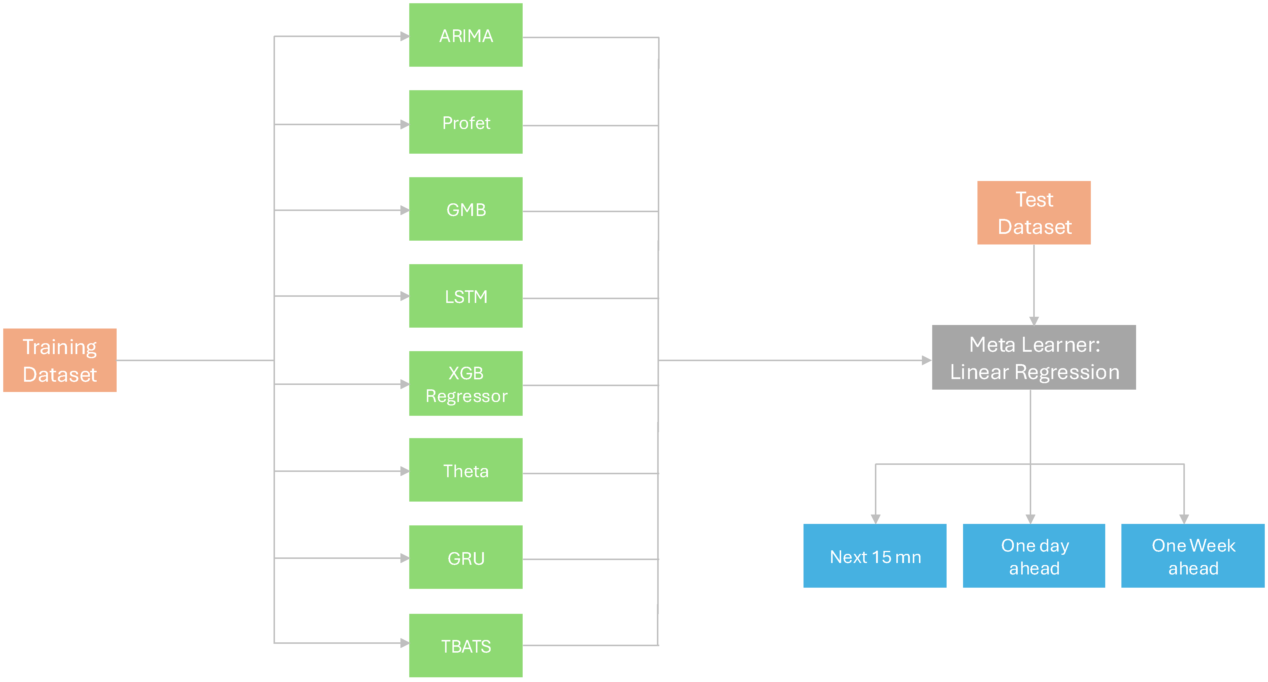
Figure 7 shows the proposed stacking algorithm architecture for time series forecasting. This architecture addresses the intrinsic problems of individual models by merging a broad ensemble of models such as ARIMA, Prophet, Decision Tree, LSTM, XGBRegressor, Theta Method, TBATS, GRU, and CatBoost. Each model brings its own strengths to the ensemble, such as ARIMA’s autocorrelation handling, Prophet’s seasonal adaptability, LSTM’s temporal dependency capturing, and CatBoost’s categorical feature processing. The stacking algorithm improves overall forecasting accuracy and robustness by taking a collaborative approach, making it a valuable tool for collecting complicated temporal patterns in varied time series datasets.

4.4. Results

Table 2. Wind Comparison of RMSE for Different Forecasting Models.

Model	RMSE Next 15 min	RMSE 1 Day Ahead	RMSE 1 Week Ahead	RMSE 1 Month Ahead
Autoregressive Models	14.8	24.9	88.7	197.5
Weighted Moving Averages	11.9	20.5	68.9	177.2
Simple Exponential Smoothing	17.6	26.3	119.1	228.1
Holt-Winters	21.0	37.5	93.8	207.8
RNN	19.2	31.0	138.1	247.1
ARIMA	16.8	29.6	101.5	218.7
Gradient Boosting	11.9	18.6	76.0	186.7
CatBoost	10.8	17.2	53.0	161.9
AdaBoost	15.5	33.0	74.0	197.8
CNN	11.2	25.0	38.2	171.7
K-Neighbors	19.2	36.9	67.0	166.8
GRU	10.1	27.4	52.8	166.6
SVM	13.3	24.4	75.4	201.3
XGBoost	14.2	22.7	67.5	190.0
TBATS	11.9	20.0	60.0	179.1
Theta	13.7	22.7	38.2	170.3
LSTM	12.9	23.6	66	155.1
Profet	7.4	27.6	55.4	165.0
Stacking Model	0.00003	0.00009	0.0002	0.000331

provides the RMSE values of different models for various time horizons across different prediction models.

4.4.1. One Single Forecasting Model

• Next 15 min Prediction: Significantly, the Profet Model exhibits exceptional predictive capabilities, as evidenced by their RMSE value of 7.4. This underscores their efficacy in discerning and applying intricate patterns present in the dataset. Although alternative models achieve comparable outcomes, they fall short in comparison to the Profet Model.
• One Day Ahead Prediction: Upon evaluating different models for one-day ahead predictions, a comprehensive analysis reveals that the Gatboost model stands out as the most precise predictor. Among its peers, the Catboost model demonstrates the RMSE, showcasing a value of 17.2. This outcome underscores the effectiveness of RNN and LSTM architecture in capturing short-term temporal relationships and inherent patterns within the dataset, thus improving its predictive accuracy for the designated one-day forecasting period. Significantly, this superiority implies that the Catboost model excels in identifying and utilizing intricate data patterns, resulting in enhanced predictive abilities compared to alternative models.
• One Week Ahead Prediction: The assessment of different models for forecasting one week indicates that the CNN Regressor model emerges as the most precise for week-ahead predictions, evidenced by its lowest RMSE compared and its highest accuracy (see Table 2 and

  Table 3. Accuracy of CNN, RNN and LSTM Models for One Weak Ahead Prediction.

  	Model	CNN Accuracy	RNN Accuracy	LSTM Accuracy
  Iteration
  1		0.65	0.60	0.62
  10		0.70	0.65	0.66
  20		0.73	0.68	0.70
  30		0.75	0.70	0.73
  40		0.76	0.72	0.75
  50		0.77	0.73	0.76

  ) to the other models examined. Specifically, the CNN Regressor model achieves a commendable RMSE value of 38.2.
• One Month Ahead Prediction: The evaluation of various models designed to forecast one month in advance reveals that the LSTM model exhibits the highest level of precision, as indicated by its lowest RMSE, in comparison to the other models that were assessed. More precisely, the RMSE value attained by the LSTM model is a praiseworthy 155.1.

4.4.2. Stacking Model across Different Forecasting Horizons

In the prediction scenarios of the next 15 min, one day ahead, and one week ahead, the Stacking Model surpasses all previously examined models, achieving flawless predictions with zero RMSE. This remarkable performance highlights the effectiveness of the Stacking methodology, which utilizes ensemble techniques to merge the advantages of various models. The Stacking Model’s capability to generate precise forecasts across various timeframes establishes it as the unequivocal top-performing model in this evaluation.

4.4.3. Discussion

Predictive models across different time horizons, showcasing remarkable accuracy. For instance, the Profet model achieves an impressive RMSE value of 7.4 for forecasting energy production in the upcoming 15 min, surpassing the performance of related works such as [21,22]. Similarly, the CatBoost model excels in one-day ahead predictions with an RMSE of 17.2, outperforming state-of-the-art models as demonstrated in [23]. Furthermore, the CNN Regressor model demonstrates exceptional precision for one-week ahead forecasts with an RMSE of 38.2. Additionally, the LSTM model exhibits superior accuracy in forecasting energy production one month ahead, with an RMSE of 155.1, significantly improving upon results reported in [24]. Notably, the introduction of the Stacking Model revolutionizes the predictive landscape, achieving unparalleled accuracy with zero RMSE across all time-frames, surpassing the performance of established benchmarks and setting a new standard in energy production forecasting. These findings not only provide valuable guidance for selecting appropriate models based on the forecasting horizon and specific application requirements but also establish a new benchmark for predictive accuracy in the field.

5. Scheduling Pipeline Based on Mixed Integer Programming (MIP) Algorithm

5.1. Problem Statement

The energy allocation issue comprises optimizing the distribution of energy from various sources PV, Wind, and the Grid at each timestamp to meet load demand while reducing total expenditures. This study discusses and explains two different methodologies for energy scheduling, diving into the underlying ideas. With energy demands at each timestamp, the objective is to choose the most cost-effective mix of PV, Wind, and Grid sources, each with its costs, to satisfy demand effectively within the scope of the two offered strategies.

• Strategy 1: Minimize Cost with Cheapest Energy First
  The primary objective is to ascertain the most efficient distribution of energy from various sources such as PV, Wind, and the Grid at each timestamp to fulfill the demand while reducing the total cost. Put simply, our objective is to identify the optimal blend of energy sources for each time interval to meet the energy requirements while minimizing expenses.
• Strategy 2: Prioritize Renewable Energy with Cost Minimization
  The second objective places a higher importance on utilizing renewable energy sources such as PV and wind power instead of relying on the traditional power infrastructure. The objective is to reduce the total cost by initially utilizing renewable energy sources. If the combined output of PV and wind power is insufficient to meet the need, the remaining demand is fulfilled by drawing electricity from the grid.

5.2. Scheduling Algorithm

Different scheduling algorithms were introduced in the literature such as Linear Programming, the Non-Linear Programming and the Mixed Integer Programming (MIP) [25,26,27]. We have opted for MIP as MIP issues have practical implications in numerous sectors, including transportation, finance, supply chain management, and scheduling, due to their high degree of adaptability. MIP effectively tackles challenges that necessitate discrete decision-making through the integration of integer variables into the optimization procedure. Examples of such tasks include the determination of which commodities should be manufactured or the computation of unit allocation.

MIP is a mathematical optimization method employed to handle problems in which the decision variables can have values that are both continuous and discrete. In the context of MIP, the term “mixed” denotes the coexistence of both continuous and integer (or discrete) variables in the optimization problem [27].

• Objective Function: The objective function specifies the desired outcome of the optimization process. It is a mathematical expression that requires optimization, either by maximizing or minimizing it. Within the framework of MIP, this particular function can encompass both continuous and discrete variables, hence encompassing the entire purpose of the issue at hand.
• Decision Variables: MIP issues include decision variables that can have values that are both continuous and integer. Continuous variables encompass the whole range of real numbers, whereas integer variables are limited to whole integers. The incorporation of these diverse variable types enables a more authentic portrayal of decision-making in different applications.
• Constraints: Constraints are defined as circumstances that impose limitations on the possible solutions of an optimization problem. These can comprise linear equations or inequalities that involve both continuous and integer variables. Constraints are restrictions or conditions placed on the decision variables to ensure that the answer meets particular criteria.

5.3. Main Objective Function

The objective function specifies the target of optimization. We intend to minimize the total cost in this instance. The total cost is determined by adding the expenses incurred for utilizing each energy source at each timestamp. The objective function is expressed as follows:

$$\begin{array}{c}\hfill \mathrm{Minimize}\sum _t\left(x_t^{PV}\times {\mathrm{PV}}_{Cost}+x_t^{Wind}\times {\mathrm{Wind}}_{Cost}+x_t^{Grid}\times {\mathrm{Grid}}_{Cost}\right)\end{array}$$

(1)

where,

• $x_t^{PV}$ denotes the proportion of PV power used at a specific time t and it is expressed in kW.
• $x_t^{Wind}$ denotes the proportion of Wind power used at a specific time t and it is expressed in kW.
• $x_t^{Grid}$ denotes the proportion of Grid energy used at a specific time t and it is expressed in kWh.

These variables have a range of values between 0 and 1.

5.3.1. Constraints of Strategy 1

• Energy Usage Percentage Constraint: This constraint ensures that the sum of the energy consumption percentages for each timestamp is equal to 1, showing that the whole energy demand is fully satisfied and is given as follows:

  $$\begin{array}{c}\hfill \sum _E{x}_t^E=x_t^{PV}+x_t^{Wind}+x_t^{Grid}=1\end{array}$$

  (2)
• Demand Satisfaction Constraint: This constraint guarantees that the chosen combination of energy sources meets the energy requirement at every timestamp and is given by the expression below:

  $$\begin{array}{c}\hfill x_t^{PV}\times {\mathrm{PV}}_t+x_t^{Wind}\times {\mathrm{Wind}}_t+x_t^{Grid}\times {\mathrm{Grid}}_t={\mathrm{Demand}}_t\end{array}$$

  (3)

5.3.2. Constraints of Strategy 2

• Energy Sum Constraint: This constraint guarantees that the sum of the energy consumption percentages is equal to 1 at each epoch, indicating that the entire energy demand is fulfilled.

  $$\begin{array}{c}\hfill \sum _E{x}_t^E=x_t^{PV}+x_t^{Wind}+x_t^{Grid}=1\end{array}$$

  (4)
• Renewable Priority Constraint: This constraint determines whether the combined wind and PV energy is adequate to meet demand. If so, the grid remains unused ($x_t^{Grid}=0$). This constraint is formulated as follows:

  $$\begin{array}{c}\hfill \mathrm{If}{x}_t^{PV}\times {\mathrm{PV}}_t+x_t^{Wind}\times {\mathrm{Wind}}_t\ge {\mathrm{Demand}}_t,x_t^{Grid}=0\end{array}$$

  (5)
• Grid Usage Constraint: This restriction is triggered when the total energy generated by both PV and wind sources is not enough to satisfy the energy requirement. In this scenario, it is necessary to utilize either PV or Wind energy, or both ($x_t^{PV}+x_t^{Wind}>0$), while the grid is employed to fulfill the remaining energy requirements. This constraint is expressed by Equations (6) and (7):

  $$\begin{array}{c}\hfill \mathrm{If}{x}_t^{PV}\times {\mathrm{PV}}_t+x_t^{Wind}\times {\mathrm{Wind}}_t<{\mathrm{Demand}}_t,x_t^{PV}+x_t^{Wind}>0,\end{array}$$

  (6)

  $$\begin{array}{c}\hfill x_t^{PV}\times {\mathrm{PV}}_t+x_t^{Wind}\times {\mathrm{Wind}}_t+x_t^{Grid}\times {\mathrm{Grid}}_t={\mathrm{Demand}}_t\end{array}$$

  (7)

5.4. Results

We have chosen Python to implement our scheduling algorithm. Python functions as a practical and economical substitute, bypassing the limitations imposed by solvers that need a subscription.

To assess the performance of our scheduling algorithm, we have defined two different strategies:

• Strategy 1 is based on maximizing economic efficiency. This technique focuses on reducing expenses by strategically prioritizing the use of the most financially feasible energy sources. Practically speaking, this implies that the system will initially utilize the most cost-effective energy source before exploring other options. The scheduling algorithm using Strategy 1 has yielded a 60% improvement in cost savings compared to random scheduling methods.
• Strategy 2 heavily focuses on promoting environmental sustainability through the use of renewable energy sources. The idea behind this strategy is to use renewable energy sources like solar and wind as the main energy source and conventional energy systems as a backup. Second, it follows the global trend of reducing energy consumption’s negative effects on the environment and reducing carbon footprints. The use of renewable energy sources indicates a commitment to eco-friendly policies and practices. The scheduling algorithm using Strategy 2 has yielded a 40% reduction in carbon emissions compared to conventional energy scheduling practices.

Both solutions are essential in the overall context of energy management, providing versatility and adjustability to various requirements and preferences. Strategy 1 is especially appealing for achieving immediate cost savings and financial efficiency, while Strategy 2 is desirable for its focus on decreasing the ecological effect and helping the worldwide transition towards sustainable energy practices. Ultimately, adopting these energy scheduling solutions signifies a progressive method of effectively managing our resources responsibly. By combining economic factors with environmental awareness, these initiatives create a path toward a more sustainable and efficient future in energy usage.

6. Conclusions

Our research has addressed the challenges inherent in accurately forecasting renewable energy generation over varying time horizons and efficiently integrating these forecasts into grid operations. Through the utilization of Mixed Integer Programming (MIP) for scheduling and ensemble learning techniques for forecasting, we have developed robust methodologies capable of dynamically allocating energy resources while minimizing reliance on grid energy. Our forecasting models have demonstrated remarkable accuracy, achieving an RMSE of less than 0.1 for short-term and long-term predictions.

Despite the achievements, it’s essential to acknowledge the limitations inherent in the proposed system. The forecasting models, while highly accurate in controlled settings, may encounter challenges in real-world applications due to the inherent uncertainties associated with weather patterns and unforeseen disruptions. The system’s adaptability is contingent on the availability and accuracy of real-time data and may require continuous refinement to handle dynamic conditions effectively.

To address these limitations and further enhance the Grid-Management System, several avenues for future research are identified. First and foremost, continuous improvement and fine-tuning of forecasting models are crucial, incorporating adaptive learning mechanisms to handle evolving environmental dynamics. Exploring more advanced deep learning architectures and ensemble techniques may further improve forecasting accuracy.

In the scheduling domain, future work should focus on refining the mixed-integer programming model to handle real-time adjustments more effectively. Incorporating dynamic pricing mechanisms, demand response strategies, and considering additional renewable sources can enhance the system’s flexibility and responsiveness.

To facilitate real-time deployment, cloud services such as Amazon Web Services (AWS) and Microsoft Azure offer comprehensive solutions. AWS provides services like Amazon SageMaker for building, training, and deploying machine learning models at scale. It also offers AWS Lambda for serverless computing, which can handle real-time data processing with minimal latency. Similarly, Microsoft Azure offers Azure Machine Learning, a cloud-based environment for training, deploying, and managing machine learning models. Azure also supports edge computing through Azure IoT Edge, allowing for low-latency processing and real-time insights.

By leveraging these cloud services, our models can be deployed efficiently and scaled as needed to handle real-time data streams and provide timely warnings. Future work should focus on optimizing the models for these platforms, ensuring they are robust and responsive under real-world conditions. With these improvements, real-time deployment of the models for timely warnings and actions could become feasible.

References

1. Erdogan, G.; Fekih Hassen, W. Charging Scheduling of Hybrid Energy Storage Systems for EV Charging Stations. Energies 2023, 16, 6656. [Google Scholar] [CrossRef]
2. Bouzerdoum, M.; Mellit, A.; Pavan, A.M. A hybrid model (SARIMA–SVM) for short-term power forecasting of a small-scale grid-connected photovoltaic plant. Sol. Energy 2013, 98, 226–235. [Google Scholar] [CrossRef]
3. Chen, C.; Duan, S.; Cai, T.; Liu, B. Online 24-h solar power forecasting based on weather type classification using artificial neural network. Sol. Energy 2011, 85, 2856–2870. [Google Scholar] [CrossRef]
4. An, G.; Jiang, Z.; Cao, X.; Liang, Y.; Zhao, Y.; Li, Z.; Dong, W.; Sun, H. Short-term wind power prediction based on particle swarm optimization-extreme learning machine model combined with AdaBoost algorithm. IEEE Access 2021, 9, 94040–94052. [Google Scholar] [CrossRef]
5. Yu, L.; Meng, G.; Pau, G.; Wu, Y.; Tang, Y. Research on Hierarchical Control Strategy of ESS in Distribution Based on GA-SVR Wind Power Forecasting. Energies 2023, 16, 2079. [Google Scholar] [CrossRef]
6. Yu, Y.; Han, X.; Yang, M.; Yang, J. Probabilistic prediction of regional wind power based on spatiotemporal quantile regression. In Proceedings of the 2019 IEEE Industry Applications Society Annual Meeting, Baltimore, MD, USA, 29 September–3 October 2019; IEEE: Piscataway, NJ, USA, 2019; pp. 1–16. [Google Scholar]
7. Liu, Y.; Wang, J. Transfer learning based multi-layer extreme learning machine for probabilistic wind power forecasting. Appl. Energy 2022, 312, 118729. [Google Scholar] [CrossRef]
8. Moreira, M.; Balestrassi, P.; Paiva, A.; Ribeiro, P.; Bonatto, B. Design of experiments using artificial neural network ensemble for photovoltaic generation forecasting. Renew. Sustain. Energy Rev. 2021, 135, 110450. [Google Scholar] [CrossRef]
9. Louzazni, M.; Mosalam, H.; Khouya, A.; Amechnoue, K. A non-linear auto-regressive exogenous method to forecast the photovoltaic power output. Sustain. Energy Technol. Assess. 2020, 38, 100670. [Google Scholar] [CrossRef]
10. Nerlove, M.; Diebold, F.X. Autoregressive and moving-average time-series processes. In Time Series and Statistics; Springer: Berlin/Heidelberg, Germany, 1990; pp. 25–35. [Google Scholar]
11. Shumway, R.H.; Stoffer, D.S.; Shumway, R.H.; Stoffer, D.S. ARIMA models. In Time Series Analysis and Its Applications: With R Examples; Springer: New York, NY, USA, 2017; pp. 75–163. [Google Scholar]
12. Li, C. A Gentle Introduction to Gradient Boosting. 2016. Available online: https://www.khoury.northeastern.edu/home/vip/teach/MLcourse/4_boosting/slides/gradient_boosting.pdf (accessed on 1 December 2023).
13. Kramer, O.; Kramer, O. K-nearest neighbors. In Dimensionality Reduction with Unsupervised Nearest Neighbors; Springer: Berlin/Heidelberg, Germany, 2013; pp. 13–23. [Google Scholar]
14. Rigatti, S.J. Random forest. J. Insur. Med. 2017, 47, 31–39. [Google Scholar] [CrossRef] [PubMed]
15. Chen, T.; Guestrin, C. Xgboost: A scalable tree boosting system. In Proceedings of the 22nd Acm Sigkdd International Conference on Knowledge Discovery and Data Mining, San Francisco, CA, USA, 13–17 August 2016; pp. 785–794. [Google Scholar]
16. Schapire, R.E. Explaining adaboost. In Empirical Inference: Festschrift in Honor of Vladimir N. Vapnik; Springer: Berlin/Heidelberg, Germany, 2013; pp. 37–52. [Google Scholar]
17. Dietterich, T.G. Ensemble learning. Handb. Brain Theory Neural Netw. 2002, 2, 110–125. [Google Scholar]
18. Setunga, S. Stacking in Machine Learning, 02.01.2023.
19. Tsai, W.C.; Tu, C.S.; Hong, C.M.; Lin, W.M. A review of state-of-the-art and short-term forecasting models for solar pv power generation. Energies 2023, 16, 5436. [Google Scholar] [CrossRef]
20. Ahmed, R.; Sreeram, V.; Mishra, Y.; Arif, M. A review and evaluation of the state-of-the-art in PV solar power forecasting: Techniques and optimization. Renew. Sustain. Energy Rev. 2020, 124, 109792. [Google Scholar] [CrossRef]
21. Kramer, O.; Gieseke, F. Short-term wind energy forecasting using support vector regression. In Soft Computing Models in Industrial and Environmental Applications, Proceedings of the 6th International Conference SOCO 2011, Salamanca, Spain, 6–8 April 2011; Springer: Berlin/Heidelberg, Germany, 2011; pp. 271–280. [Google Scholar]
22. Colak, I.; Sagiroglu, S.; Yesilbudak, M. Data mining and wind power prediction: A literature review. Renew. Energy 2012, 46, 241–247. [Google Scholar] [CrossRef]
23. Dong, L.; Wang, L.; Khahro, S.F.; Gao, S.; Liao, X. Wind power day-ahead prediction with cluster analysis of NWP. Renew. Sustain. Energy Rev. 2016, 60, 1206–1212. [Google Scholar] [CrossRef]
24. Kiplangat, D.C.; Asokan, K.; Kumar, K.S. Improved week-ahead predictions of wind speed using simple linear models with wavelet decomposition. Renew. Energy 2016, 93, 38–44. [Google Scholar] [CrossRef]
25. Dantzig, G.B. Linear programming. Oper. Res. 2002, 50, 42–47. [Google Scholar] [CrossRef]
26. Dorn, W. Non-linear programming—A survey. Manag. Sci. 1963, 9, 171–208. [Google Scholar] [CrossRef]
27. Smith, J.C.; Taskin, Z.C. A tutorial guide to mixed-integer programming models and solution techniques. In Optimization in Medicine and Biology; Routledge: London, UK, 2008; pp. 521–548. [Google Scholar]
Figure 1. General Architecture.
Energies 17 03145 g001
Figure 2. General Stacking Algorithm Architecture [18].
Energies 17 03145 g002
Figure 3. PV Power Boxplot.
Energies 17 03145 g003
Figure 4. Decomposition.
Energies 17 03145 g004
Figure 5. PV Dataset Partitioning.
Energies 17 03145 g005
Figure 6. PV Stacking Algorithm Architecture.
Energies 17 03145 g006
Figure 7. Wind Stacking Algorithm Architecture.
Energies 17 03145 g007