An Artificial Neural Network Model for a Comprehensive Assessment of the Production Performance of Multiple Fractured Unconventional Tight Gas Wells

Abstract

The potential of unconventional hydrocarbon resources has been unlocked since the hydraulic fracturing technique in combination with long horizontal wells was applied to develop this type of reservoir economically. The design and optimization of the fracturing treatment and the stimulated reservoir volume and the forecasting of production performance are crucial for the development and management of such resources. However, the production performance of tight gas reservoirs is a complicated nonlinear problem, described by many parameters loaded with uncertainty. The complexity of the problem influences and inspires the sophistication of the solution to be used. This paper proposed an artificial network model that allows for fast, extended, and accurate analyses of the production performance of multiple fractured unconventional tight gas wells. In the comprehensive approach developed, the reservoir rock parameters, the drainage area, and the hydraulic fracture parameters are treated as a variable input to the model. The analysis is no longer constrained by fixed “shoes box” geometry, and the values of the parameters defining the reservoir and stimulated volume are not limited to a few discrete values. The numerical experiment used to construct a database for model development was designed using a genetically optimized Latin hypercube sampling technique. A special approach was used in the preparation of “blind data”, which are crucial for truly reliable model verification. In the result, a developed tool offers an extended rock-fluid description, flexible model, and stimulated reservoir volume dimensioning and parameterization, as well as a high degree of applicability in sensitivity analysis and/or optimization.

1. Introduction

During the ongoing energy transition towards a net-zero economy, a continuous increase in demand for natural gas is observed. Global natural gas and LNG storage capacity in import markets is expected to expand by 10% (or 45 bcm) during the 2023–2028 period, largely supported by projects in China; Europe and Eurasia [1] also seem to confirm that the importance of natural gas will remain for at least several more decades. However, a decline in conventional resources resulted in interest in low-quality resources, classified as unconventional. The potential of unconventional hydrocarbon resources has been unlocked with the hydraulic fracturing technique in combination with horizontal wells, making production from shales and tight sandstones economical. Holditch’s forecast on the increasingly important role of unconventional resources [2] has been fulfilled, at least in the United States and Canada. The leaders are being chased by China with its huge potential and an intensive increase in the production of unconventional tight gas [3]. Long, multiple fractured horizontal wells (MFHW) are the basis for the success of unconventional hydrocarbon reservoirs. However, horizontal drilling and massive multistage fracturing are cost-intensive techniques. Therefore, design and optimization of the fracturing treatment and the stimulated reservoir volume parameters and the forecasting of production performance are crucial for the development and management of unconventional hydrocarbon resources. However, the production performance of tight gas reservoirs is a complicated non-linear problem, described by many parameters loaded with uncertainty.

The typical approach used in sensitivity analysis regarding the effects of hydraulic fracture parameters on unconventional gas production is to use the so-called “shoes box” numerical model with fixed dimensions and fixed-length horizontal well. Then, the number of fractures (or fracture spacing), fracture half-length, and permeability are varied throughout the analysis. If the effects of the drainage area are to be investigated, the number of cases is limited as this requires preparation of new models, and the number of simulation runs increases. Frequently, performance evaluations were carried out for a single value of the main reservoir parameters such as depth, thickness, porosity, initial water saturation, initial reservoir pressure, and reservoir temperature. The usefulness and generalizability of the results obtained appear to be significantly reduced. Moreover, according to Byrnes [4], the fundamental requirement for effective gas production from low-permeability sandstones is understanding their in situ petrophysical properties, the most important of which are porosity, brine saturation, and effective gas permeability at reservoir brine saturation. The false assumption regarding the values for these petrophysical properties can result in improper development and, thus, significant costs.

Bagherian et al. [5] used three box-shaped models differentiated with respect to the drainage area and four horizontal section lengths with a number of fractures ranging from one to ten; the horizontal permeability varied with three values with a rather limited extent ($k_h=[2.000,2.924,3.684]\mathsf{\mu }\mathrm{D}$. However, the same reservoir thickness, hydraulic fracture spacing, and length, as well as initial reservoir pressure, porosity, and relative permeability curves, were used in all models of the analysis performed.

Owolabi et al. [6] proposed a fairly extensive simulation-based sensitivity analysis study for unconventional reservoirs with four models with 5, 10, 20, and 40 hydraulic fractures, respectively, that were run with different permeabilities (10 values from 1 nD to 1 mD), fracture half-lengths (305 m and 1220 m), drainage areas (7 values from 80 to 1275 acres), and fracture conductivities (7 values from 0.305 to 3050 mD · m). It should be noted that with the applied permeability range, this study covers reservoirs better than typical tight sandstones on one side and reaches values typical for gas shales on the other side. However, reservoir depth, thickness, porosity, and water saturation, as well as reservoir temperature and initial reservoir pressure, were fixed for all models in the study. The relative permeability curves are not discussed; therefore, it should be assumed that one set of curves was used.

MoradiDowlatabad et al. [7] used statistical algorithms coupled with numerical reservoir simulations to evaluate the simultaneous impacts of important pertinent parameters on the performance of different MFHW designs at various production periods. They applied Latin hypercube sampling and Eclipse 100 black oil simulator, nevertheless fixed external dimensions of the model, along with fixed porosity, reservoir depth, temperature, and initial reservoir pressure, were used in all simulated cases.

Such a simplified approach to sensitivity analysis/performance assessment is obviously valuable as general conclusions can be drawn; however, it seems undeniable that the sound framework for the design of SRV should be case-dedicated and must incorporate the given reservoir characteristics, original gas in place, rock–fluid characteristic, etc. These are related to the petrophysical characteristic of the reservoir rock, initial reservoir conditions, and reservoir volume to be produced. In the case of nanodarcy shale gas reservoirs, it could be argued that the performance of MFHW is based mainly on the inflow from the stimulated reservoir volume (SRV), and the out-of-SRV zone does not contribute significantly to production performance (if at all). However, with respect to gas accumulations in tight sandstones with microdarcy permeability, this assumption may not be acceptable, as gas inflow from outside of the SRV is very likely to occur on a scale that cannot be neglected. Therefore, the solid performance assessment and/or sensitivity analysis should incorporate not only the SRV parameters but also the interaction of the SRV with the reservoir volume outside the SRV. In other words, different acreages (drainage areas) and SRV configurations should be analyzed for a given reservoir.

The assessment of production performance in unconventional resources has also been addressed with artificial intelligence (AI) tools. Kalantari-Dahaghi et al. [8] presented an artificial-neural-network-based proxy model that had the ability to reproduce well-based numerical simulation responses for shale gas with high accuracy, but for a relatively short period of production equal to 1 year.

Recently, Wang et al. [9] used AI tools to predict the production performance of MFHW in unconventional oil reservoirs. In their approach, the authors used numerical simulation to generate a database that was used to develop a deep belief network model. The input parameters of the model varied within predefined variability ranges; however, the variability of each parameter was limited to a few discrete values. Such an approach results in repeating the same value of the given parameter between cases within the designed sample, and hence, the representation of the problem space is limited. Moreover, such an unrestricted sampling produces unreasonable and improbable combinations of parameter values that must be removed manually before being presented to the network. The authors used Monte Carlo to populate the database with 1000 cases, and after cleaning, it consisted of 946 cases.

Since tight gas production in China plays an increasingly greater role, increased interest in applying AI tools for fractured horizontal tight gas well productivity predictions is observed there, for example, by combining field data with traditional decline curve analysis and machine learning, as presented in [10,11].

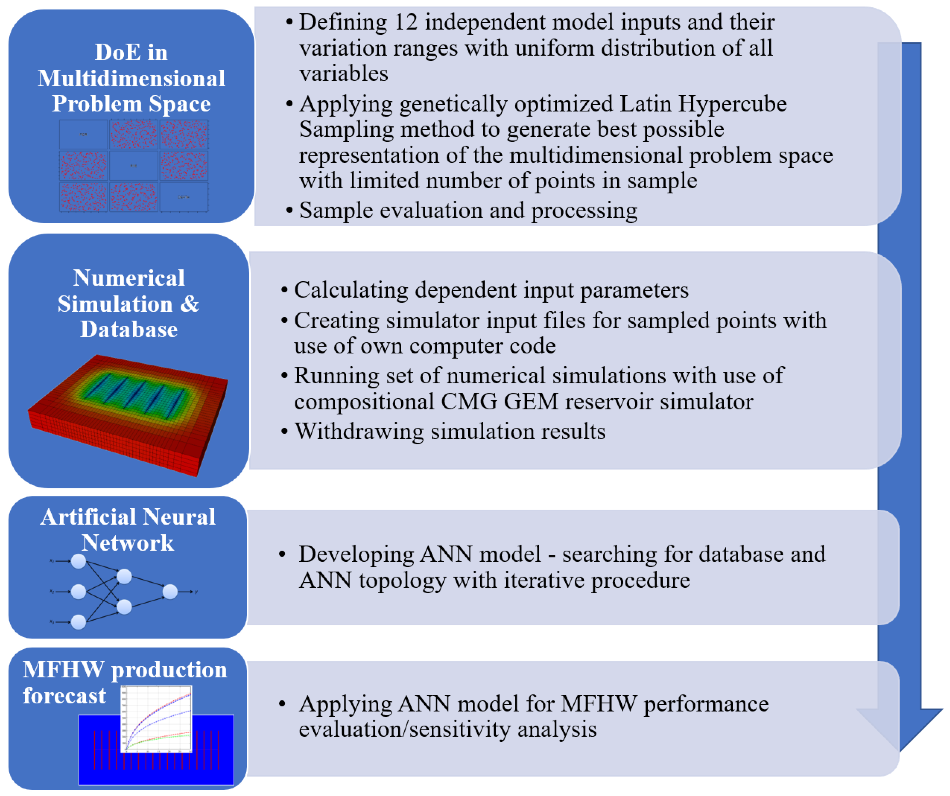
The purpose of this study was to develop a comprehensive methodology and a useful tool to go beyond the limitations described above and allow for the evaluation of the performance of multiple fractured horizontal wells in tight gas reservoirs dynamically and comprehensively by integrating AI tools with the sound reservoir engineering. It was decided to use an artificial neural network and “feed” it with data generated with the use of a numerical simulator. At each stage of the process of developing the ANN model, emphasis was placed on including as many elements as possible that have not been included in a coherent methodology so far. Furthermore, the condition of limiting the sample size, i.e., the number of numerical simulations and, thus, the computational cost of database, was assumed. The consequence of this approach is the need to maximize the quality of the sample. This issue is also addressed in this study and implemented.

In this study, the reservoir rock parameters, the external dimensions of the investigated reservoir volume (drainage area), and the hydraulic fracture parameters (i.e., the parameters defining SRV) are assumed to be the variable input of the model. The reservoir rock is characterized with the use of dedicated correlations to ensure a realistic representation of the reservoir conditions and flow of the reservoir fluids under specific conditions of hydraulically fractured tight sandstones. Each of the numerical models used in the development of the ANN model has been prepared based on the set of independent input parameters (those sampled within the design of experiment procedure) and dependent input parameters (i.e., those calculated based on the independent ones). Within the proposed approach, the “shoes box” was not fixed but was created individually, with the use of a developed dedicated computer code for each point (simulation run) sampled from the problem space.

The problem space was defined to allow for a range of variability wide enough to make the developed tool practical, on the one hand, and not to lose accuracy, on the other. Much attention was paid to designing a numerical experiment, which is crucial to ensuring the quality of the sample that represents the multidimensional problem space with a limited number of points. For this purpose, Latin hypercube sampling optimized using genetic algorithms was applied.

The general workflow of the proposed new approach is shown in Figure 1.

2. Methods

This work uses the unconventional and compositional GEM reservoir simulator to simulate the production of multiple fractured horizontal gas wells from a tight gas reservoir. GEM is the industry-standard reservoir simulator developed by the Computer Modelling Group (CMG). The problem space is defined with 12 parameters that vary within predefined ranges of variability. The numerical experiment, i.e., the set of points sampled from within the problem space, is sampled with the use of the Latin hypercube sampling method (LHS) optimized with a genetic algorithm. Cumulative gas curves are generated using the numerical simulator and act as target data for an artificial neural network trained for input data from a numerical experiment.

2.1. Problem Space and Numerical Simulation Models

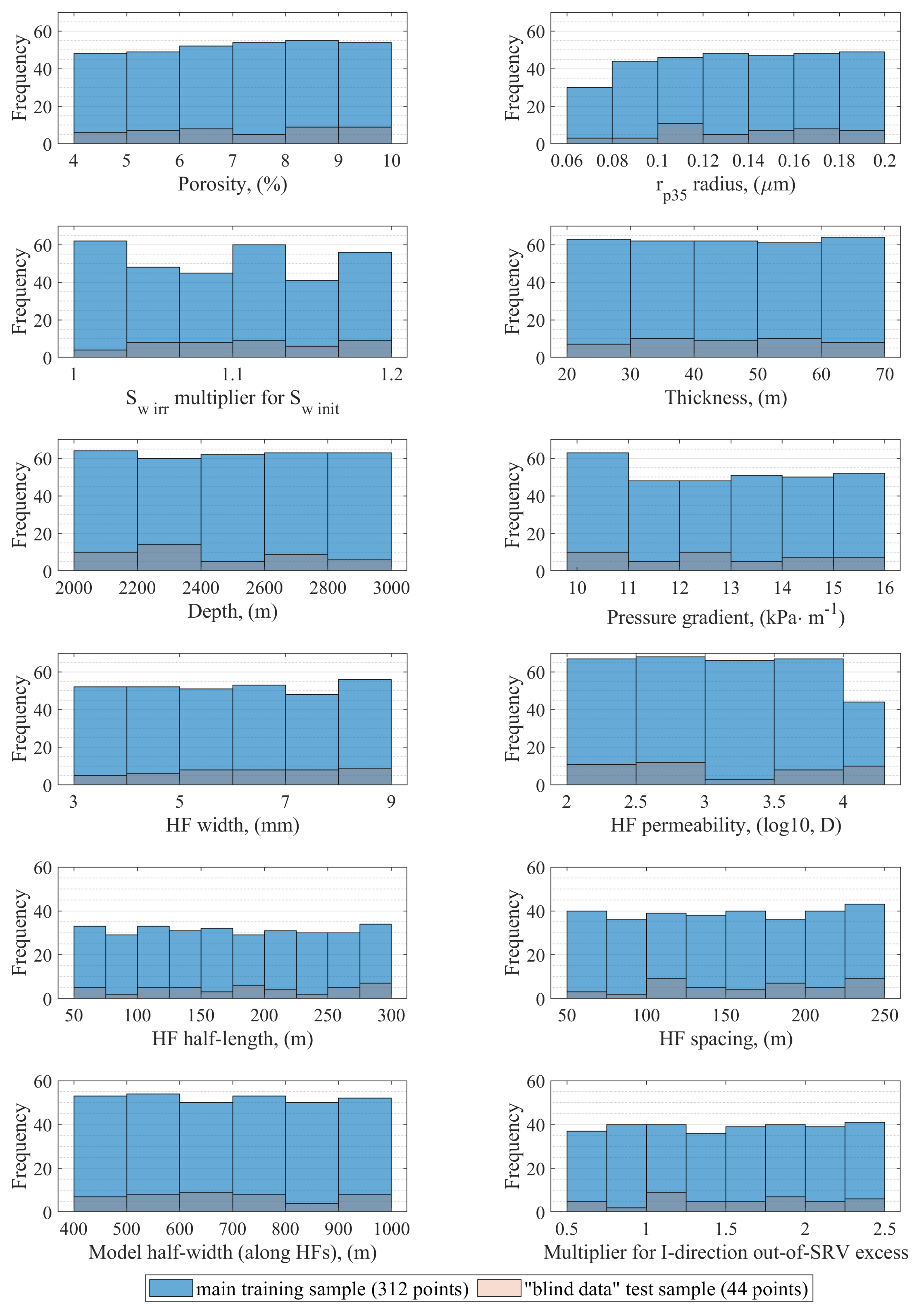
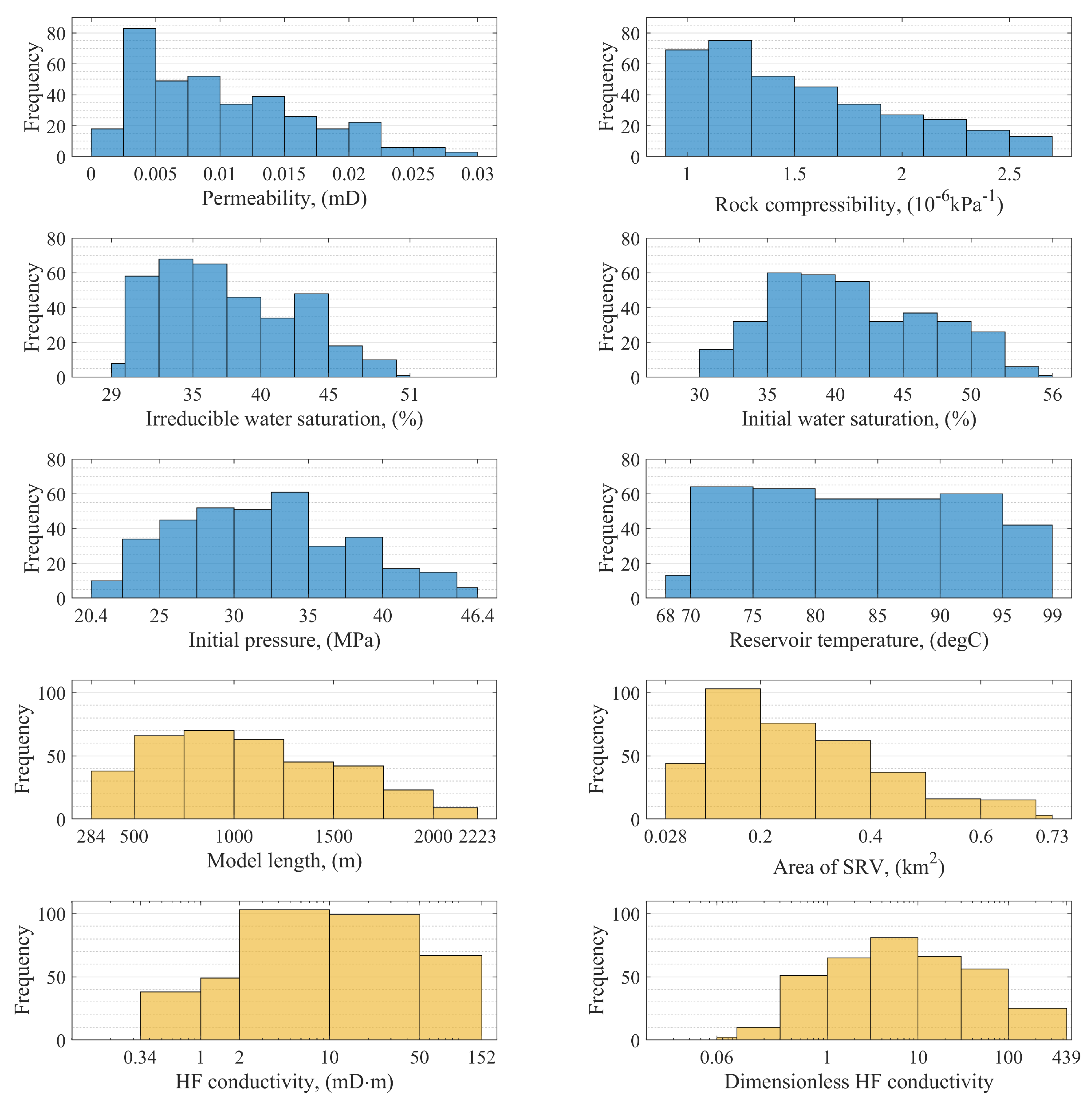
The database used to train and test the artificial neural network model was generated with the use of the industry standard CMG-GEM reservoir simulator. For internal purposes of this study, the input parameters were divided into two groups herein called independent input variables, which are sampled within the design of experiment (DoE) procedure, and dependent input variables, which are calculated based on the independent ones. The independent inputs were varied within their ranges of variability, and uniform distributions were assumed to obtain as much information on the defined problem space as possible. All input variables were divided into three groups with respect to (1) reservoir rock, (2) hydraulic fractures and stimulated reservoir volume, and (3) lateral dimensions of the investigated area (external model dimensions) or acreage, and are listed with their variation ranges in

Table 1. The selected parameters of the reservoir and the stimulated reservoir volume—independent input variables sampled from within the problem space.

Parameter	Unit	Range
Reservoir
Porosity	%	4.0–10.0
Pore throat radius, $r_{p35}$	$\mathsf{\mu }$m	0.06–0.20
Initial water saturation (as $S_{wirr}$ multiple)	-	1.00–1.20
Thickness	m	20–70
Pressure gradient	kPa·m−1	9.8–16.0
Depth to the top	m	2000–3000
Stimulate reservoir volume
Hydraulic fracture spacing	m	50–250
Hydraulic fracture half-length	m	50–300
Hydraulic fracture aperture	mm	3.0–9.0
Hydraulic fracture permeability	D	0.1–20.0
Areal model dimensions (acreage)
Width	m	400–1000
Length from left and right boundary to first and last HF, respectively (as HF spacing multiple)	-	0.5–2.5

. It is worth highlighting that variability is not limited to a few discrete values within the predefined range, but values are sampled from the whole predefined range with a reasonable number of decimal places.

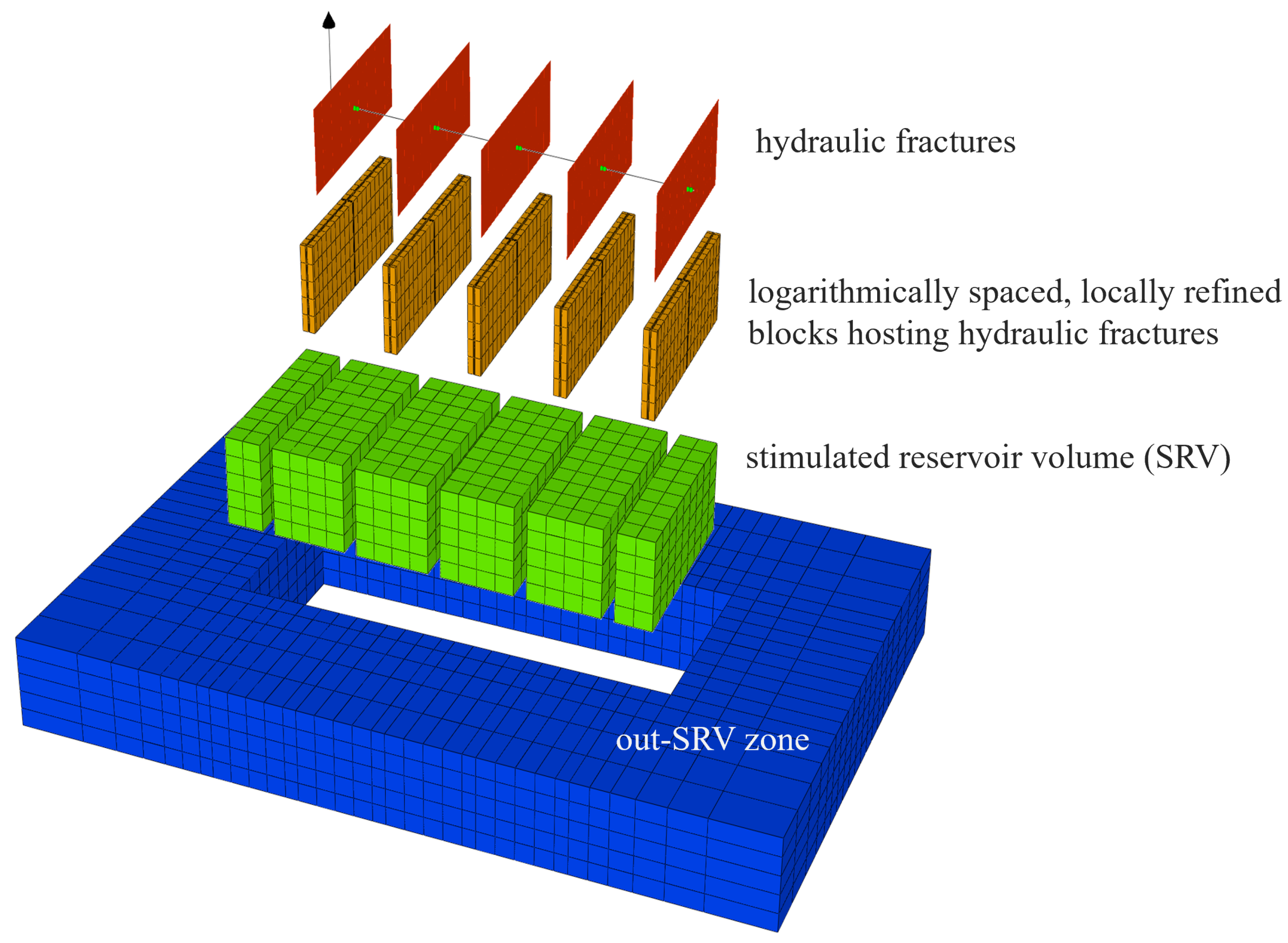
The numerical simulation model for single multiple fractured horizontal well production from the tight gas reservoir comprises:

(1)

stimulated reservoir volume with areal extent defined by the product of hydraulic fracture spacing multiplied by the number of fractures and total fracture length;

(2)

locally refined, logarithmically spaced grid blocks hosting hydraulic fractures [12];

(3)

hydraulic fractures (original blocks divided into five subblocks with the central ones representing hydraulic fractures);

(4)

out-of-SRV zone, where the excess length in the direction parallel to the well (on both sides of the model) has been dimensioned in relation to the fracture spacing.

The hydraulic fractures are modeled using locally refined, logarithmically spaced grid blocks according to the method presented extensively in [12] and adopted in CMG’s GEM simulator. In this approach, grid refinement is limited to blocks hosting hydraulic fractures and does not extend outside the SRV, limiting the number of computational blocks in the model. Non-Darcy flow within these highly conductive channels is incorporated as well.

The well is perforated only in the blocks that house the fracture, and the loss of pressure along the lateral is neglected. Elements of the model in 3D decomposition are shown in Figure 2.

The simplest approach with respect to hydraulic fracture conductivity in sensitivity/performance analysis is to assume a fixed average aperture for hydraulic fractures across all models within the analysis and to compensate by varying fracture permeability to obtain desirable conductivity. As fracture conductivity is the product of fracture permeability and fracture width (aperture), the same conductivity can be obtained for different aperture–permeability combinations. Although this approach seems to be justified in terms of conductivity, it is not when it comes to the water (fracturing fluid) that remains in the fractures after fracturing. To properly account for the amount of fracturing fluid in hydraulic fractures and the duration of backflow periods, in this study, both fracture permeability and width were treated as variables and not only fracture conductivity.

The average width of the fracture was assumed to take values from 3 to 9 mm together with a constant porosity of the propped fracture of 40%. To ensure that the effects of hydraulic fracture permeability are captured, in this study, it changes from 100 mD to 20,000 mD. Because permeability changes over a very wide range, sampling on a logarithmic scale was adopted. This allowed me to avoid the trap of a seemingly even distribution and efficiently test the entire range of variability.

In ultralow-permeability gas reservoirs in shales, the contrast between hydraulic fracture permeability and reservoir permeability is usually high enough to effectively transport fluid flowing from the reservoir through fractures to the well [13]. Fractures with the same permeability (or conductivity) behave completely differently in nanodarcy shales and microdarcy tight sandstones. The performance of tight gas models is more sensitive to the ability of fractures to transport reservoir fluids [14]. Thus, dimensionless conductivity was introduced to quantitatively describe the relation between the matrix and the capacity of the fracture to transmit fluids. Fracture conductivity is the product of the proppant permeability that fills the fracture (fracture permeability), $k_f$, and the width of the fracture (aperture), $w_f$. Dimensionless conductivity, $C_{fD}$, is defined as the ratio of fracture conductivity to the product of formation (matrix) permeability, $k_m$, and fracture half-length, $x_f$.

$$\begin{array}{c}\hfill \begin{array}{c}\hfill C_{fD}=\frac{k_f{w}_f}{k_m{x}_f}\end{array}\end{array}$$

(1)

Fractures with $C_{fD}>30$ are interpreted as infinitely conductive. However, based on both Prats’ original work and industry experience, a value $C_{fD}$ of 10 continues to be widely used as a standard design factor in the industry [15,16]. This study comprises a wide range of dimensionless conductivities from as little as 0.06 to 439, where 41.0% of the models have $C_{fD}$ between 1 and 10 and 34.3% of the models have $C_{fD}$ between 10 and 100.

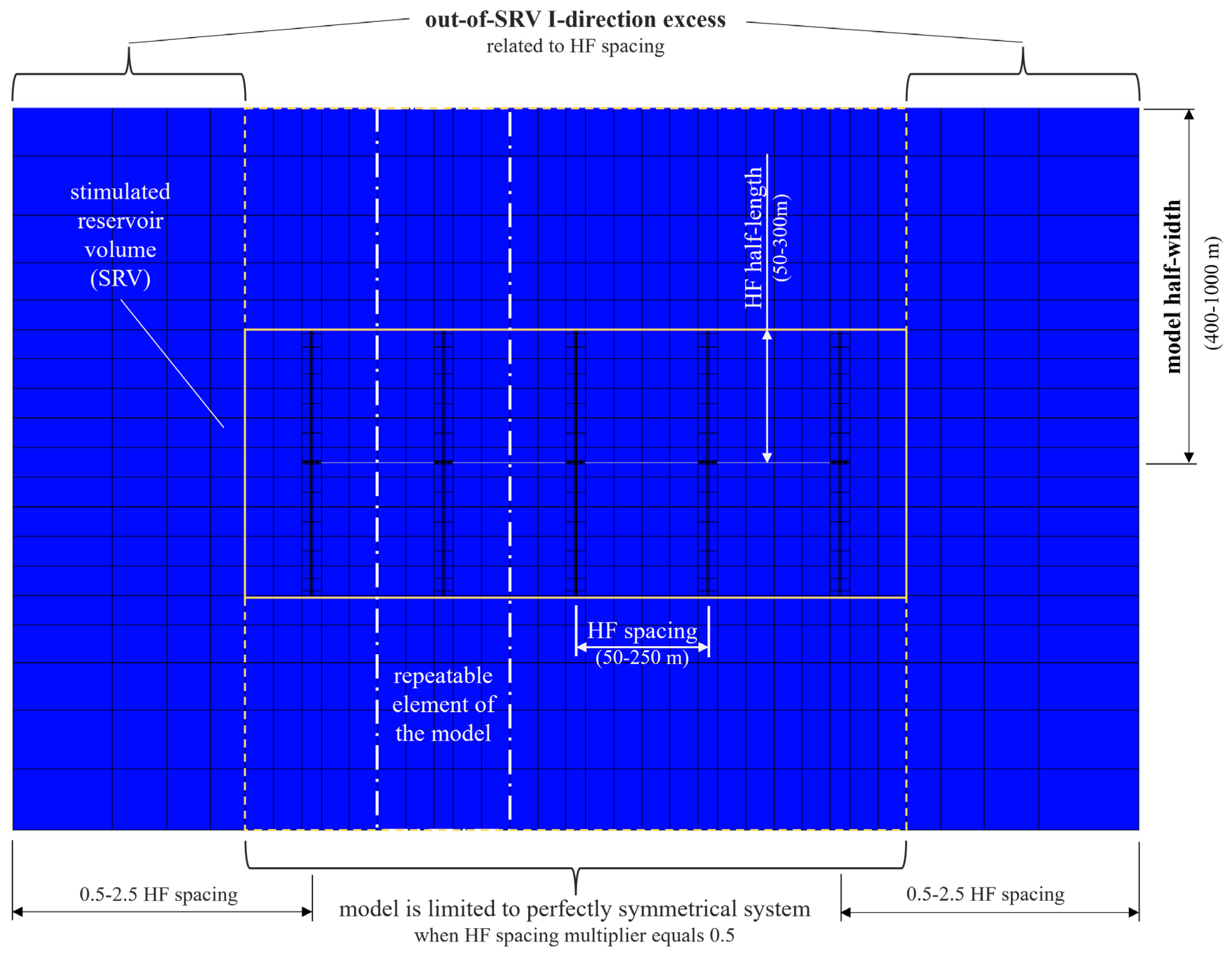
The model half-width (measured in direction parallel to hydraulic fractures) was assumed to cover the range of 400–1000 m. The length of the model was related to the hydraulic fracture spacing using a dedicated multiplier that allowed control of the distance from the left boundary of the model to the first HF and from the last HF to the right boundary of the model (see Figure 3). Due to this approach, it is possible to assess the impact of fractures (SRV) with specific parameters on various acreages (designed dynamically in both directions outside the stimulated reservoir volume) and, thus, optimize the well spacing within the field. Furthermore, reversely, for the fixed “shoes box”, a number of fracture lengths can be tested.

The horizontal dimensions of the basic grid blocks are 30 m and 45 m in direction I (along the horizontal part of the well) and direction J (along the hydraulic fracture wings), respectively. However, adopting a fixed block dimension in the direction of the hydraulic fracture spacing limits the available distances to integer multiples of the block dimension, enforces discrete division of the range of spacing under investigation (which may negatively influence the quality of DoE), and thus, limits comprehensiveness of the solution. To “break free” from such a limitation, the dimensions of the blocks within the SRV—except blocks containing fractures—are adopted dynamically, allowing for unrestricted (within assumed range of variability) hydraulic fracture spacing. Furthermore, the number of blocks between two neighboring fractures is always set even to ensure symmetry. Outside the SRV the dimensions of the blocks in both directions increase geometrically to reduce the overall number of blocks and, thus, the numerical simulation runtime and cost.

Regarding the reservoir thickness, to ensure computational comparability between individual models making up the numerical experiment, thicknesses of the layers comprising each model are selected in such a way that they are as close as possible to 10 m with an odd number of layers (to always locate the well exactly in the middle of the model). Any differences resulting from rounding are compensated in the middle layer of the model.

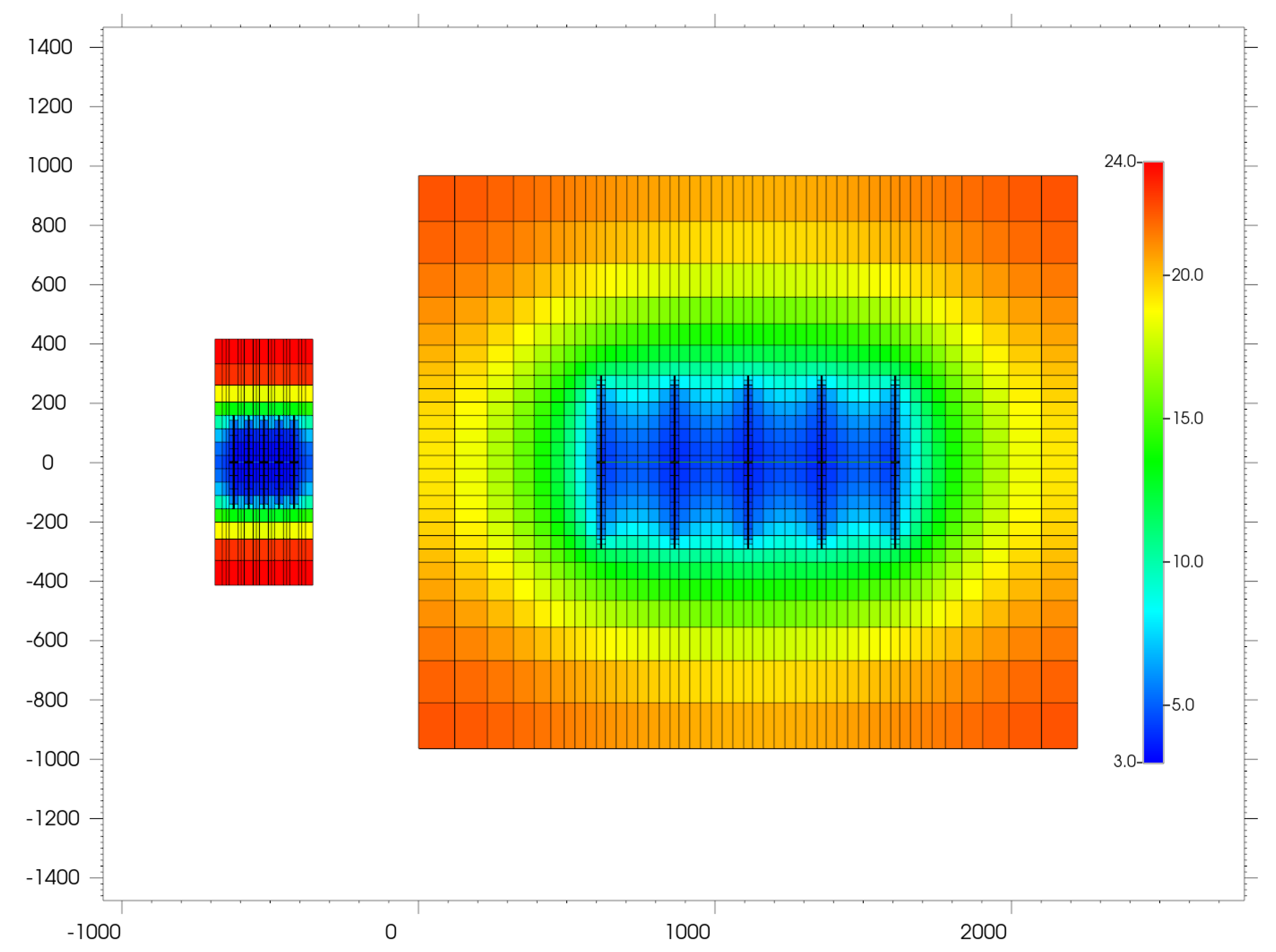
To illustrate the complexity of the task resulting from a wide range of parameter variability, Figure 4 shows two models from both ends of the incorporated variability range when it comes to acreage. This also illustrates the wide range of applicability of the developed model.

2.1.1. Porosity and Permeability

Table 1 lacks some key reservoir parameters, e.g., permeability and water saturation. These obligatory parameters have not been defined directly, as is usually practiced. In this study, the reservoir rock was characterized by its effective porosity and radius of the pore throat $r_{p35}$, as described in [17]. The concept of $r_{35}$, that is, the radius of the pore throat at mercury saturation of 35% from the mercury injection capillary pressure (MICP) measurement, was developed by H.D. Winland [18,19] and is widely used as a rock typing method [17,20,21]. Using Winland’s equation, the pore throat aperture can be calculated on the basis of porosity and permeability. Aguilera modified the Winland correlation using data from more than 2500 sandstone and carbonate samples [22,23]:

$$r_{p35}=2.665{\left(\frac{k}{\varphi }\right)}^{0.45},$$

(2)

where $r_{p35}$ is the approximated dimension of the pore channel in micrometers, k is permeability (mD), and $\varphi$ is porosity (%). Based on $r_{p35}$, the pore channels are classified into five groups [17]:

• megapores, $r_{p35}>10\mathsf{\mu }$m;
• macropores, $r_{p35}\in (2.5-10)\mathsf{\mu }$m;
• mesopores, $r_{p35}\in (0.5-2.5)\mathsf{\mu }$m;
• micropores, $r_{p35}\in (0.1-0.5)\mathsf{\mu }$m;
• nanopores, $r_{p35}\in (0.01-0.1)\mathsf{\mu }$m.

In this study, porosity and $r_{p35}$ have both been assumed to be independent input variables subjected to sampling from predefined variation ranges. Then the permeability of the reservoir rock matrix was calculated on the basis of correlation (2). Adopting this approach allowed for a comprehensive investigation of the behavior of reservoirs with the same porosity but with different pore structures represented by $r_{p35}$. However, this was not the only reason to apply this approach. Describing reservoir rock with porosity and permeability directly may result in an undesired (improbable and un-physical) combination of, e.g., relatively low porosity with improbably high permeability when it comes to the design of the experiment. Linking permeability to porosity by $r_{p35}$ allowed us to have only reasonable and probable combinations (at least, justified by empirical correlation) of these essential parameters in a numerical experiment. Therefore, the description of the reservoir rocks tends to be more reliable and physical, and DoE was not confounded by internally inconsistent data. Incorporating such points within the database could impede training and/or lead to the inappropriate generalization of knowledge presented to the artificial neural network.

2.1.2. Irreducible and Initial Water Saturation

Before hydrocarbons migrating from source rocks are trapped, reservoir rocks are usually “fully” saturated with water ($S_w=100\%$) and the minimum pressure, called threshold pressure/pore entry pressure, of the gas is needed to breach the surface tension of the larger pores, and the replacement of water by gas begins. In conventional highly permeable reservoirs, threshold pressures are relatively low and hydrostatic pressure differences allow gas invasion into the reservoir rock. In tight reservoirs, the pore throats are much smaller, the surface tension of the wetting fluid is higher, and consequently, the threshold pressures are usually higher. Therefore, additional pressure must be provided to achieve gas penetration into the reservoir. Furthermore, to achieve typical water saturations for these reservoirs, gas columns of $1000m$ or more are generally needed [24]. Thus, the capillary pressure was probably not the result of the height of the gas and water columns, but the gas pressure developed during its expulsion from the source rock. According to Crotti [24], this mechanism explains typical properties of tight gas reservoirs, such as overpressurization, anomalous water gradients, and isolated reservoirs with their own final conditions. As a consequence, no transition zones are expected and the concept of free water level is irrelevant in tight gas reservoirs. The final water saturation and, therefore, the original gas in place are governed by the maximum overpressurization in the geological history of the reservoir and the extent of the reservoir is defined by the sedimentary structure itself [24]. However, tight sandstones might not be as tight at the time of gas filling. According to [4], it is possible for a reservoir to have been charged with gas early in its burial history, when the rock properties were better, and with subsequent burial and diagenesis, the rock properties changed.

In result, water saturation in tight reservoirs is expected to be relatively high—much higher than in conventional reservoirs, and as porosity decreases and rock becomes “tighter”, the difficulty in saturation measurements increases. Low-permeability sandstones are typically characterized by high capillary pressure and high irreducible water saturation ($S_{wirr}$). The correlations of $S_{wirr}$ with porosity and permeability provide a useful model for approximate predictions of $S_{wirr}$ [25]. In this study, the correlation developed for the Medina Formation and the Mesaverde-Frontier Formation tight sandstones [25] was used:

$${log}_{10}\left(S_{wirr}\right)=-0.187+{log}_{10}\left(k_{\infty }\right)+1.18,$$

(3)

where $S_{wirr}$ is in percent and k in mD.

The initial water saturation is one of the parameters that affect the original gas in place and the flow of fluids in the reservoir. In the case of a tight gas reservoir, it depends both on the petrophysical characteristic of the rock and the geological history of the reservoir. The method presented here takes into account a possible initial water saturation greater than irreducible water saturation. The initial water saturation can be equal to or greater than the irreducible water saturation calculated specifically for the reservoir characterized by porosity and $r_{p35}$. The procedure for determining horizontal permeability, irreducible water saturation, and initial water saturation is summarized in Figure 5.

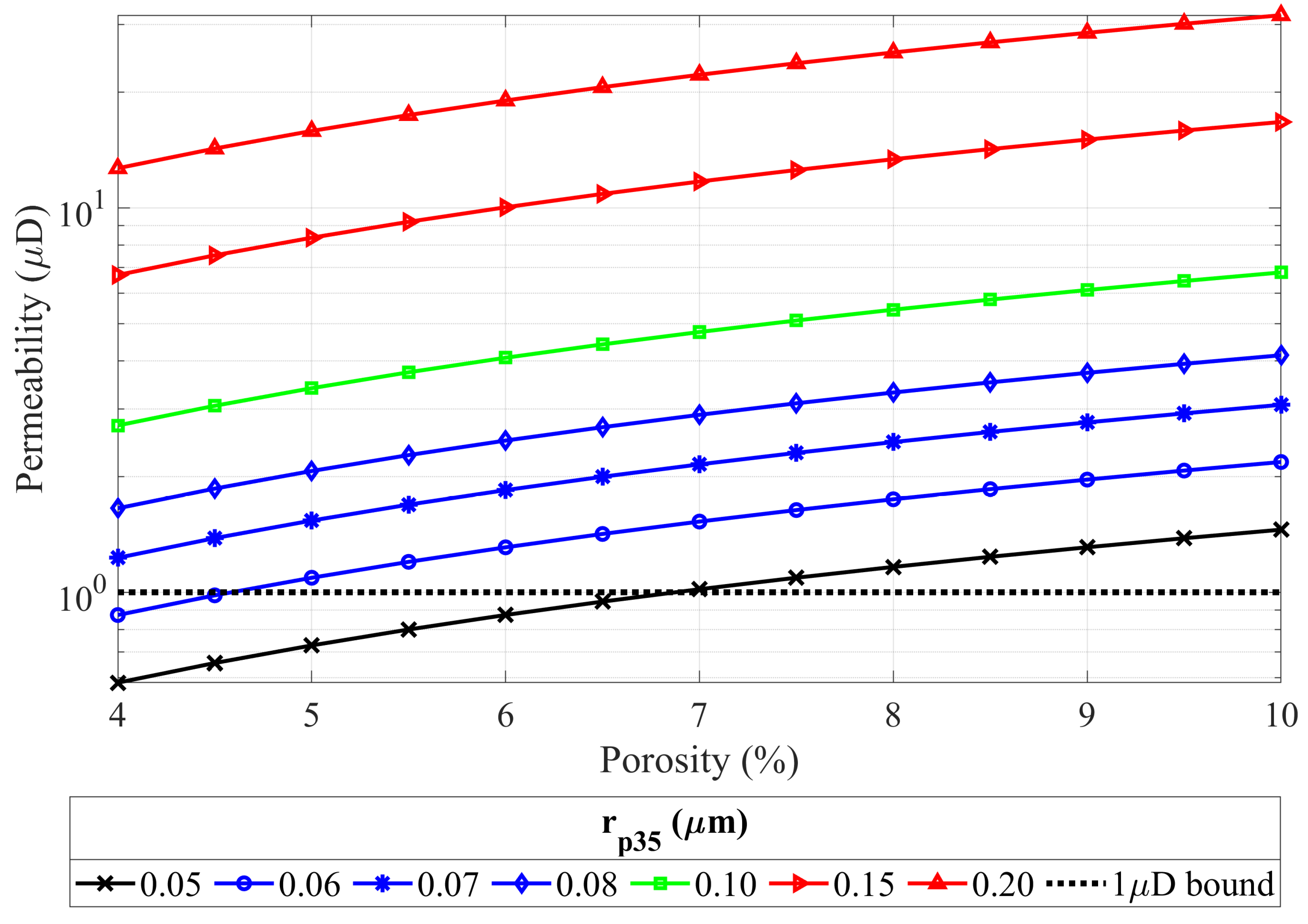
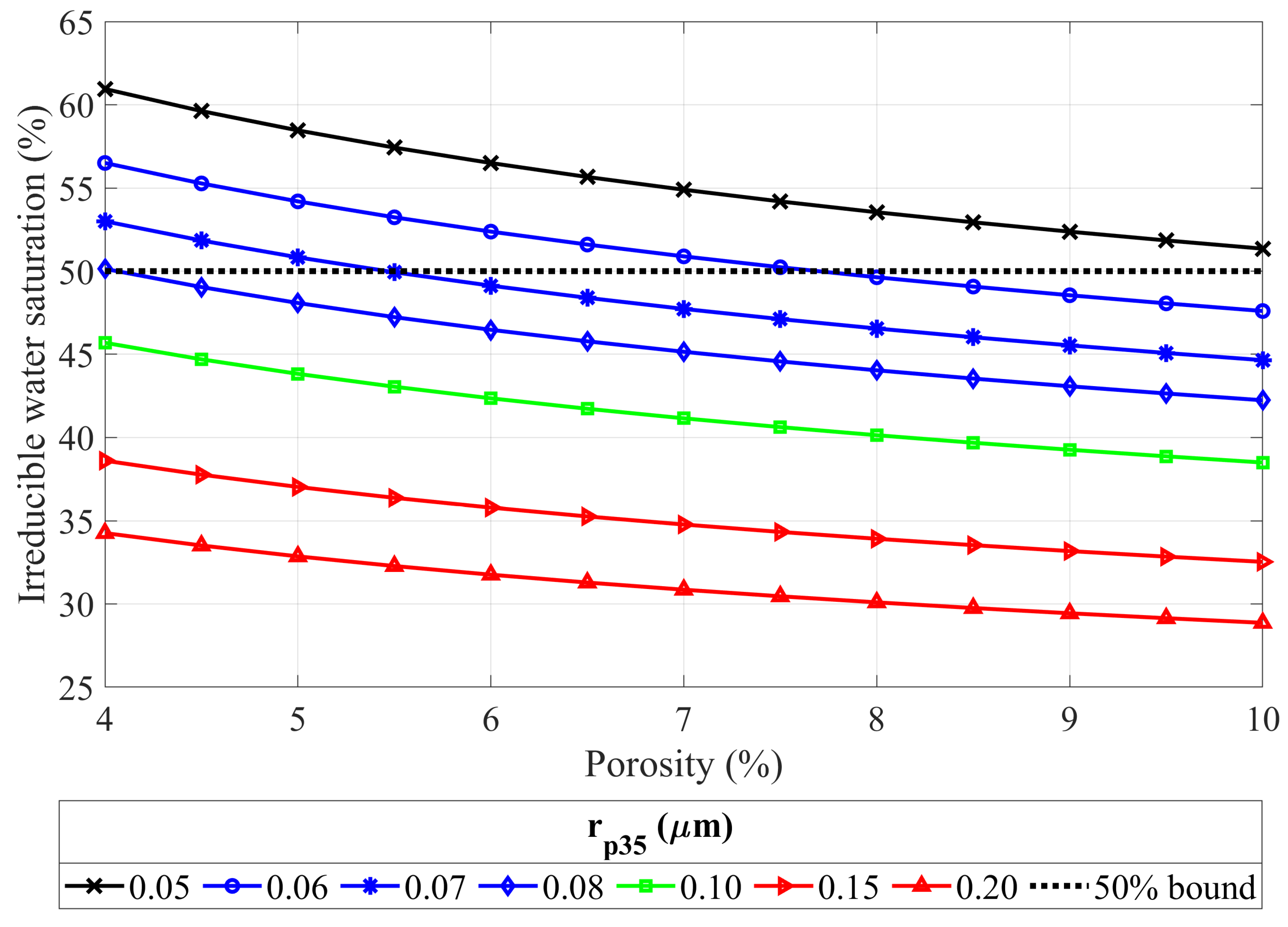
The porosity range of 4–10% was assumed for the analysis. For the radius of the pore throat of $0.05\mathsf{\mu }$m, the resulting permeabilities are lower than $1\mathsf{\mu }$D ($0.001$ mD) for a porosity lower than 7% (see Figure 6). More importantly, for the same $r_{p35}$, the irreducible water saturation exceeds 50% for the whole porosity range and exceeds 60% for the lower limit of porosity (see Figure 7). Such a high water saturation in combination with low porosities results in a very low original gas in place. (Of course, the amount of gas in place depends on the reservoir thickness, too, and in some particular situations, this may be of interest). Initially, the lower limit of $r_{p35}$ was taken to be as low as $0.05\mathsf{\mu }$m. However, during the development of the ANN model, it was observed that the runs with the lowest pore throat were definite outliers in the negative sense. To keep the tool developed consistently and ensure the quality of the results obtained, it was decided to narrow the investigated range of pore throat variability and put rocks with $r_{p35}<0.06\mathsf{\mu }$m beyond the scope of this study. Therefore, the range of values of $r_{p35}$ was limited to 0.06–0.20 $\mathsf{\mu }$m and, hence, partially covers the “upper” part of the nanopores and the “lower” part of the micropores, according to the classification presented above.

The compressibility of the rock (pore volume) was modeled using the well-known Neumann correlation [26]:

$$c_{por}=\frac{97.32·{10}^{-6}}{{(1+55.8721\varphi )}^{1.42859}},$$

(4)

where $\varphi$ is in percent and $c_{por}$ in $ps{i}^{-1}$.

2.1.3. Relative Permeability Curves

Relative permeability curves play an extremely important role in modeling multiphase flows, distributing the permeability between phases depending on saturation. When dealing with microdarcy permeabilities and high water saturations, rock–fluid data require special attention. The data measured directly on samples representing reservoirs of interest are the most valuable input to the simulation model. However, such data are not always available. The relative permeability curves of the Corey type are widely accepted as an input for numerical simulations when the measured data are lacking [27].

The water permeability is progressively less than the Klinkenberg permeability with decreasing permeability for values less than 1 mD following the general relation [25,27,28]:

$$k_w={k_{\infty }}^{1.32},$$

(5)

The water permeability to the absolute Klinkenberg permeability ratio is then given with

$$\frac{k_w}{k_{\infty }}={k_{\infty }}^{0.32}.$$

(6)

Ward and Morrow [27] defined $S_{wi}$ as water saturation below which $k_{rw}$ is effectively zero. Reversely, it can be interpreted as the water saturation at which the water becomes mobile, namely, $k_{rw}(S_w\ge S_{wi})>0$, and as such, here it is called the critical water saturation, $S_{wcrit}$.

The relative permeabilities for water can be calculated by the Corey wetting-phase equation but require correction with the water permeability to the absolute Klinkenberg permeability ratio [25,27]:

$$k_{rw}={\left(\frac{S_w-S_{wcrit}}{1-S_{wcrit}}\right)}^4{k_{\infty }}^{0.32}.$$

(7)

Ward and Morrow [27] concluded that the measured gas relative permeability for tight sandstones was fitted almost exactly by a form of Corey relationship used by Sampath [29]:

$$k_{rg}={\left(1-\frac{S_w}{0.7}\right)}^{1.5}\left(1-{S_w}^2\right),$$

(8)

For purposes of this work, the modified Corey equation according to [25] was used for gas relative permeability:

$$k_{rg}={\left(1-\frac{S_w-S_{wcrit}}{1-S_{gcrit}-S_{wcrit}}\right)}^p\left(1-{\left(\frac{S_w-S_{wcrit}}{1-S_{wcrit}}\right)}^q\right),$$

(9)

where $S_w$ is the water saturation, and $S_{gcrit}$ is the critical gas saturation given with equation [25]:

$$S_{gcrit}=0.15-0.05{log}_{10}{k}_{\infty },$$

(10)

In this study, it is assumed that $S_{wcrit}\approx S_{wirr}$ and that the initial water saturation, $S_{winit}$, may be higher than $S_{wirr}$. This assumption may be correct for the scenario of filling an already tight sandstone formation, as well as for the scenario of tightening a previously gas-filled reservoir (or mix of both). It should be noted that excess water saturation in this study was defined by the fraction of $S_{wirr}$. The water saturation multiplier was treated as the independent variable with values within the range of 1.00–1.20. The resulting initial water saturation was then calculated as follows:

$$S_{winit}=X_{SWI}{S}_{wirr},$$

(11)

with $X_{SWI}\in <1.00–1.20>$. Therefore, the initial water saturation can be up to 120% of the irreducible water saturation.

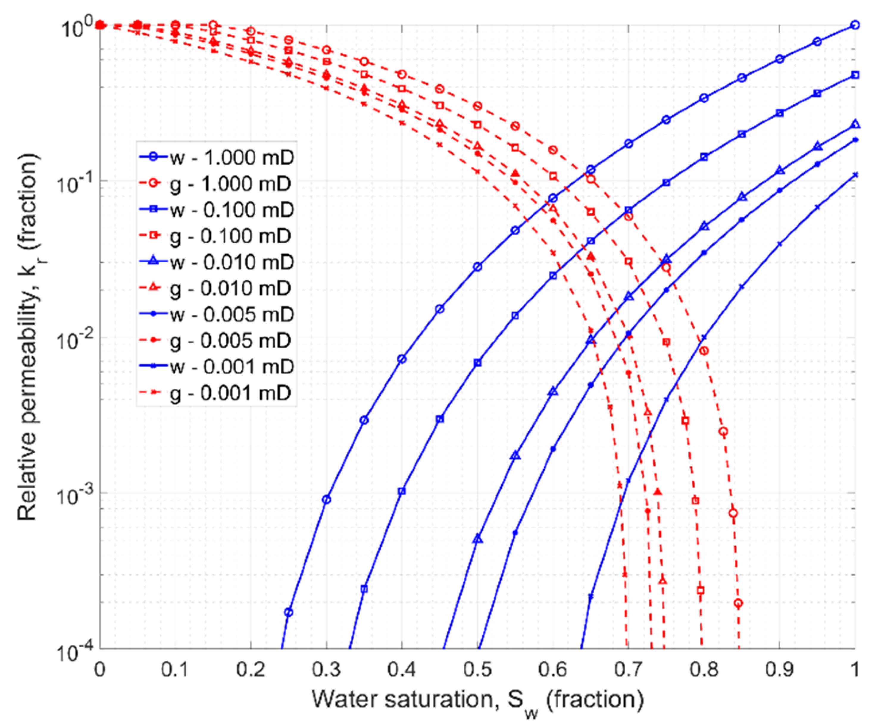
A set of $k_{rg}$ and $k_{rw}$ curves for the absolute permeability ranging from 0.001 mD to 1 mD is shown in Figure 8. The relative permeability of gas decreases slightly with increasing water saturation, while water relative permeability curves move rather significantly toward higher water saturation values.

Relative permeability tables were generated individually for each point (simulation run) of the designed numerical experiment and depend on three independent input variables: porosity, radius of the pores throat $r_{p35}$, and the multiplier of water saturation.

2.1.4. Initial Conditions and Reservoir Fluid Model

The reservoir initial conditions are treated as variables, but—again—indirectly. The initial reservoir pressure is calculated based on the model’s independent variables: reservoir depth and pressure gradient. The reservoir temperature is calculated using the reservoir depth based on the general relation

$$T_{res}=8°C+0.025\frac{°C}{m}·H,$$

(12)

where H is the depth to the top of the reservoir, in meters.

The compositional model of the reservoir fluid was applied with the Peng–Robinson equation of state (PR-EOS). The natural gas was represented with a simplified composition of methane ($80\%mole$) and ethane ($20\%mole$), ensuring a dry gas within the entire range of pressure and temperature investigated. The compositional simulator was chosen because in the methodology presented, the initial reservoir conditions are variable. Application of a black oil simulator would require a new PVT model for each simulation run sampled within the design of the experiment procedure. Although the preparation of one “universal” table covering the entire analyzed pressure range for fixed temperature would not be a problem, variable temperature makes such a solution impossible. The EOS-based compositional model offers flexibility when reservoir conditions are treated as variable model input.

2.2. Artificial Neural Networks and Database Generation Procedure

Artificial neurons that build an artificial neural network (ANN) are grouped into layers. Typically, a network has an input layer, one or more hidden layers, and an output layer. The number of neurons in the input layer corresponds to the number of parameters given as input. In turn, the number of neurons in the output layer is equal to the number of result parameters. Hidden layer neurons are responsible for data analysis (classification, pattern recognition). The synaptic weights assigned to individual inputs of the artificial neuron, $w_i$, are responsible for strengthening/weakening the signal at its inputs, $x_i$. The products of the individual signals, $x_i$, and their corresponding weights, $w_i$, are summed, and the total signal, a, called the total activation of the neuron, constitutes an argument for the activation function of the neuron, $f\left(a\right)$. The value of the activation function generated for this argument, $y=f\left(a\right)$, is the output of an artificial neuron and is fed to the subsequent neurons of the network or its output [30].

An artificial neural network model for multiple fractured horizontal wells in a tight gas reservoir was developed using MATLAB R2022b software [31]. The cascade feedforward artificial neural network was used. The transfer function applied in the hidden layers was the hyperbolic tangent sigmoid function (tansig) given with Equation (13), while the output layer was equipped with the linear function purelin.

$$f\left(a\right)=\frac{e^a-e^{-a}}{e^a+e^{-a}}$$

(13)

In addition to 12 basic input parameters, the input data for the ANN comprised additional parameters (calculated solely on the basis of the basic ones) that describe the system being modeled. The learning target was the cumulative gas versus time. The gas production profile used consists of 30 points over a 30-year period. The ANN was trained with the supervised learning scheme. The first tests were carried out using the well known Levenberg–Marquard backpropagation algorithm. Finally, the Bayesian regularization backpropagation algorithm was used.

The Bayesian regularization backpropagation is a network training function that updates the weight and bias values according to the Levenberg–Marquardt optimization. It minimizes a combination of squared errors and weights and then determines the correct combination so as to produce a network that generalizes well. The process is called Bayesian regularization [31]. The production profiles generated with the networks trained with Bayesian regularization increase smoothly without deviations.

Generalizing and simplifying, one could say that the “natural” application of artificial neural networks is to deal with big sets of data. However, if the data for ANN are generated through time-consuming numerical simulations, the cost of the database, and thus, its size, becomes an important issue. Striving to minimize the cost of the experiment, i.e., number of numerical simulations, consequently causes the need for experiment design optimization. The optimally designed experiment, with a specified number of samples, reflects the characteristics of a problem being modeled to the best possible degree. Thus, the approximate orthogonality of the input parameters and possibly best space filling, i.e., sampling points evenly distributed in the parameter space, are required. In other words, in the p dimensional Euclidean space (where p is the number of parameters), the harmonic average distance between each of the points and all other points in the experiment should be maximized, while the correlation between the points in this space should be minimized.

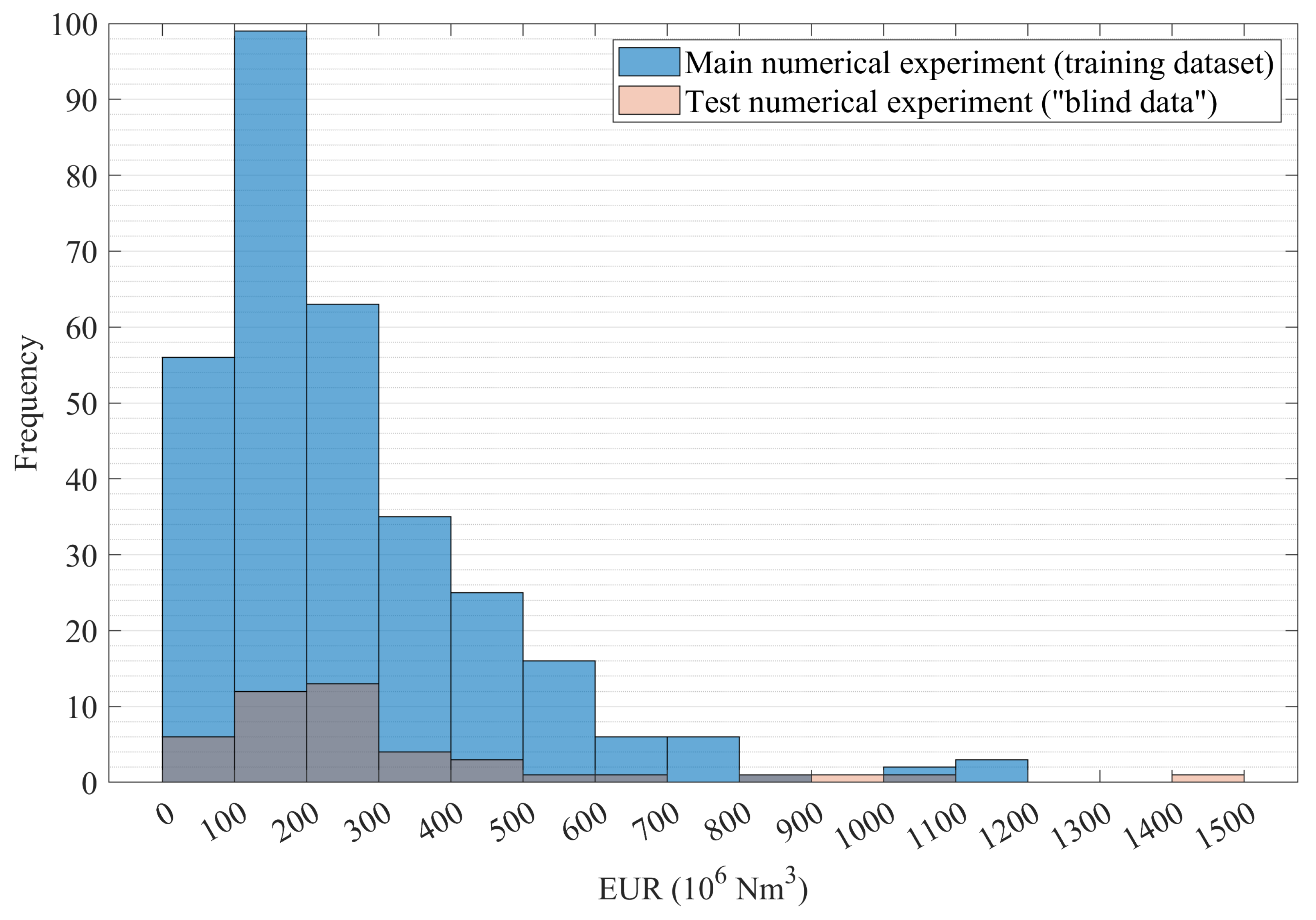
The standard procedure in artificial neural network training is to divide the dataset into three parts: (1) the training set (the biggest one), (2) the validation set used for testing during training, and (3) the test set, or so- called “blind data” for verifying the usefulness of the already trained network. However, this approach seems to conflict with the idea of optimal experiments and DoE efforts, i.e., with the imperative of minimizing and optimizing the sample.

If the initial design has a specific geometric structure (that aims at optimizing the metamodel fitting), the deletion of points from the learning sample causes the breakdown of the specific design structure while creating the new learning sample. Indeed, the new learning sample does not have the adequate statistical and geometric properties of the initial design, and the metamodel fitting process might fail. This could lead to too pessimistic quality measures [32]. Furthermore, the set of test data obtained by plucking random points from the optimal set does not represent the entire problem space; thus, the results of the test may raise objections.

For these reasons, in this study, the samples for the generation of the main training data set and the “blind data” set were designed independently as separate experiments. Using this approach made it possible to (1) preserve the specific structure of and the “load of information” carried by the sample design optimized with significant effort and (2) test the ANN model comprehensively within the whole problem space defined. Moreover, to ensure the high credibility of ANN verification, a numerical experiment for “blind data” was designed by augmenting the main Latin hypercube sample. The augmented design maintains the Latin properties of the original one; as each of the added points is not only completely different from all points of the basic design but also spread as much as possible within the problem space.

In this study, two sampling approaches were tested, both based on the Latin hypercube sampling (LHS) method. All DoE procedures were performed using R Statistical Software (version 4.3.3) [33]—a free software environment for statistical computing and graphics. In the first method (herein called the simple iteration method), the initial design was generated with the basic randomLHS procedure [34] (without any implemented optimization method), and its quality was evaluated with the minimum Euclidean distance criterion and the maximum pairwise correlation criterion. Then a new basic design was generated in the same way and compared with the previous one. If the new one was better in terms of the adopted criteria, it replaced the previous one. The procedure was repeated iteratively with 20,000 steps. The second method tested was the genetically optimized LHS (geneticLHS [35]). The genetic LHS was run with 50 designs in the initial population, 20,000 generations, and a 0.08 probability of mutation.

In addition to the aforementioned criteria (minimum distance and maximum pairwise correlation), additional sample quality assessment criteria were also used to better illustrate the difference in sample quality generated with using the compared methods; these were [36]: Scalc, coverage, meshRatio, the mean distance between sampled points, and its standard deviation.

The Scalc returns the harmonic mean of all pairwise interpoint distances. For a space-filling design, this value should be as large as possible. The coverage criterion measures whether a design is close to a regular mesh. The perfectly regular mesh is characterized by coverage = 0; therefore, a small value of coverage is desired. The meshRatio is the ratio of the largest minimum distance to the smallest minimum distance. For a perfectly regular mesh meshRatio = 1, a small value of meshRatio close to one is preferable.

3. Results and Discussion

3.1. Database

The main numerical experiment sample designed to generate the training data included 333 points (or simulation cases) in a 12-dimensional space. The orthogonality of the sample generated with geneticLHS is 4.1 times lower, and the minimum sample distance is 33.3% higher compared to the simple iterative approach described above. The sample quality measures for the compared sampling methods are summarized in

Table 2. Comparison of the design quality measures for two 333-point samples generated with simple iterative and genetically optimized Latin hypercube sampling methods.

Quality Measure	Simple Iterative LHS	Genetic LHS
Orthogonality	0.0971	0.0237
Minimum distance	0.5195	0.6923
Mean distance	1.4062	1.4121
Maximum distance	2.3511	1.9741
Distance st. dev.	0.2453	0.2078
Scalc	1.3599	1.3790
Coverage	0.1205	0.0515
meshRatio	1.9303	1.3819

. Each of them improved in genetically optimized Latin hypercube sampling compared to the simple iterative method. In light of these results, the advantage of genetically optimized sampling is overwhelming. Although the second of the methods tested is more time-consuming, it allows the generation of much better designs; hence, the genetic LHS method was used for the purpose of this study. The smaller sample (for “blind data”) designed with the use of the optAugmentLHS package [34] consisted of 40 points.

After the cut-off at initial water saturation was applied, the training data set was reduced to 312 points (simulation cases); none of the “blind data” points resulted with initial water saturation higher than the assumed cut-off value; hence, the design was not cropped. On the contrary, the sample was supplemented with additional points to extend the range of expected ultimate recovery covered by the test data. Histograms of the values sampled for each of the independent input parameters for the main experiment are shown in Figure 9, while the distribution of the resulting input parameters calculated based on them using the relations described above (herein called the dependent input parameters) is presented in Figure 10.

The distribution of the expected ultimate recovery for the main and test data sets is presented in the form of a histogram in Figure 11. Note that the individual ranges of the cumulative gas from the main training sample are well represented in the test sample. Moreover, the test sample is supplemented with the case that is a complete outlier in terms of cumulative gas, which is a challenging and meaningful test for the model.

3.2. Quality of the Developed Model

Searching for the database structure and ANN topology is a trial-and-error procedure, and the ANN model is always ”fit for purpose”. The developed model uses a cascade feedforward network with three hidden layers. A total of 356 simulation cases were used: 272 cases or 76.4% for training, 49 cases or 13.8% for validation during training, and 44 cases or 12.4% for testing and verification. A summary of ANN development is shown in Figure 12 in the form of regression graphs for each of three sets of data: training, validation, and testing. The regression graphs show a very good overall agreement between the ANN model and the numerical simulations. However, using the appropriate error metric is crucial for a proper assessment of the model quality. The most suitable for comparing time series seem to be percentage error metrics, and the mean absolute percentage error (MAPE) is one of the most popular used. It is calculated by taking the mean of the absolute difference between the actual values (numerical simulation herein) and the predicted values (ANN) divided by the actuals. Another metric used in this study is the normalized root mean squared error (NRMSE). Due to squaring, it weights large errors more than small ones, and due to the normalizing, it allows for the comparison of runs with different cumulative production. The ultimate expected recovery was used to normalize the errors in this study. The MAPE and NRMSE metrics are given with the following formulas.

$$\begin{array}{c}\hfill \begin{array}{c}\hfill MAPE=\frac{1}{n}\sum _{i=1}^n\frac{|{GP}_i^{NRM}-{GP}_i^{ANN}|}{{GP}_i^{NRM}}·100\%\end{array}\end{array}$$

(14)

and

$$\begin{array}{c}\hfill \begin{array}{c}\hfill NRMSE=\frac{\sqrt{\frac{1}{n}{\displaystyle \sum _{i=1}^n}{\left({GP}_i^{NRM}-{GP}_i^{ANN}\right)}^2}}{EUR}·100\%\end{array}\end{array}$$

(15)

where ${GP}_i^{NRS}$ and ${GP}_i^{ANN}$ are the gas produced until the i-th year of operation according to the numerical reservoir model (NRM) and the artificial neural network (ANN) model, respectively, and EUR is the expected ultimate recovery according to NRM after 30 years of operation ($EUR={GP}_{30}^{NRM}$).

The detailed distribution of the quality measures adopted (MAPE and NRMSE) is shown in Figure 13. Based on “blind data” only, the ANN model predicts the production profile with MAPE less than 6.8% and NRMSE less than 5.2%. Figure 14 presents the MAPE and NRMSE metrics in relation to cumulative gas production. The results show that (1) the highest errors are related to cases with relatively low EUR and (2) the ANN model proves its reliability for the case with EUR significantly higher than the cases used in the training. Figure 15 shows the distribution of EUR residuals (or relative errors) in the database. The maximum difference slightly exceeds 6% in both plus and minus, however, the residuals in most cases are less than 2%. A detailed comparison of three worst cases, that is, test runs with the highest MAPE value (cases 313, 320, and 322), is presented in Figure 16.

3.3. Upscaling for Higher Number of Fractures

When the distances measured from the outermost fractures to the external boundaries of the model (in the direction parallel to the horizontal well) are equal to half of the fracture spacing (multiplier equal to 0.5), the system is composed of five identical elements and perfectly symmetrical (see Figure 3). If a number of fractures greater than five is required, the internal procedure of the code comprises three steps:

(1)

running simulation for five-fracture system with desired out-of-SRV dimensions;

(2)

running simulation with the same parameters except that the out-of-SRV zone in direction I is limited to half of the fracture spacing, i.e., perfectly symmetrical system with no influence of the out-of-SRV zone,

(3)

scaling production from the above steps to the desired number of fractures.

The effect of excess volume in the out-of-SRV zones is captured in Step 1. The results obtained in Step 2 represent the production from interior fractures that are not (or negligibly) affected by the additional reservoir volume. Since running ANN is practically not time-consuming, this stepwise procedure is not a cost at all and simultaneously gives a high degree of flexibility, enabling predictions for a number of fractures restricted only by practical issues.

Unfortunately, there is some disadvantage resulting from the implemented solutions that is directly related to the maximum gas rate constraint. Multiple fractured horizontal wells in relatively good reservoirs during the initial period of operation can reach gas rates much higher than those that can be handled by typical production tubing. Thus, in practice, the gas rate is restricted based on the so-called nodal analysis that confronts the reservoir inflow performance with the vertical lift performance of the well. In this study, it was decided to incorporate the maximum gas rate constraint of $5·{10}^5$ Nm³/day for a production well. However, when a production profile for MFHW with more than five fractures is generated, the maximum gas rate constraint may not apply.

Two cases were used to validate the proposed production up-scaling procedure. Case A is based on the parameters of the simulation run number 332 and is upscaled for 18 hydraulic fractures. Case B is based on the simulation run number 330 but with the modified length of the fracture and upscaled for 16 hydraulic fractures. The input parameters for Cases A and B are summarized in

Table 3. Parameters of the extended models of cases A and B.

Parameter	Unit	Case A	Case B
		(Modified #332)	(Modified #330)
Reservoir
Porosity	%	9.11	8.06
Pore throat radius, $r_{p35}$	$\mathsf{\mu }$m	0.120	0.184
Initial water saturation (as $S_{wirr}$ multiple)	-	1.16	1.13
Thickness	m	52.22	63.55
Pressure gradient	kPa · m−1	14.81	13.30
Depth to the top	m	2168	2806
Initial reservoir pressure	MPa	32.108	37.320
Reservoir temperature	°C	62.2	78.2
Stimulated reservoir volume
Hydraulic fracture spacing	m	126	107
Hydraulic fracture half-length	m	122	240
Hydraulic fracture aperture	mm	8.1	4.8
Hydraulic fracture permeability	D	0.234	9.120
Areal model dimensions
Width	m	602	458
out-of-SRV extent (I direction)	m	266	214
Total length	m	1162	963

. The basic simulation for Case A resulted in an initial gas rate below the applied constraint of $5·{10}^5$ Nm³/day, while the simulation for Case B ran with the active constraint on the gas rate. For both cases, additional dedicated numerical models with the assumed number of fractures were prepared for comparison and full and reliable verification. Figure 17 shows the summary of the verification for cases A and B. The production profiles obtained with the ANN model and the full numerical model are compared. The quality metrics for the ANN model are calculated on the basis of full numerical models and show very good agreement with MAPE of 2.25% and 1.37% and NRMSE of 1.80% and 1.31% for cases A and B, respectively.

4. Conclusions

An efficient tool that integrates a correlation-based detailed description of a tight gas reservoir, the credibility of the industry standard technique of numerical reservoir simulation, and the impressive (and still evolving) capabilities of artificial intelligence is proposed. This combination is completed with a simple but reliable and efficient method for upscaling the basic production profile to the desired number of fractures. An ANN-based model is developed that mimics the behavior of the numerical reservoir model for MFHW in a tight gas reservoir with high accuracy and allows for the efficient analysis of production performance.

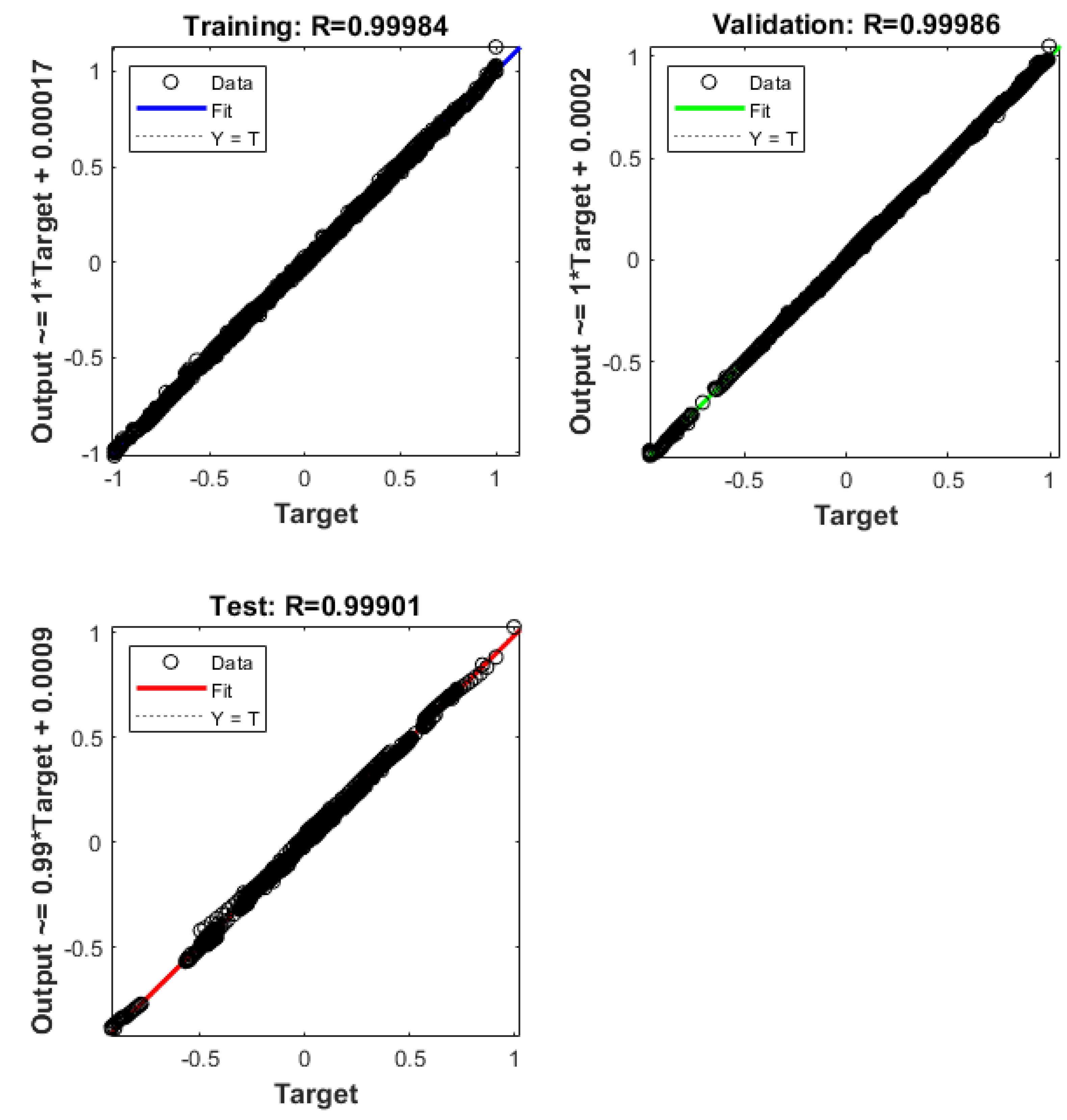
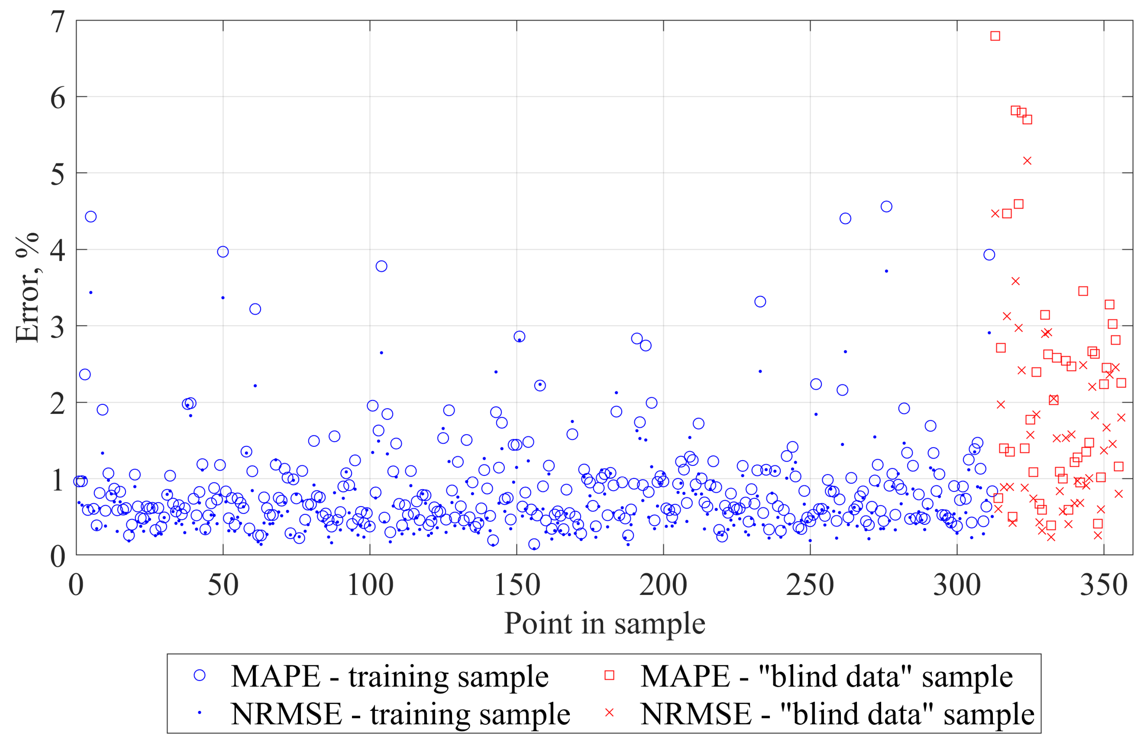
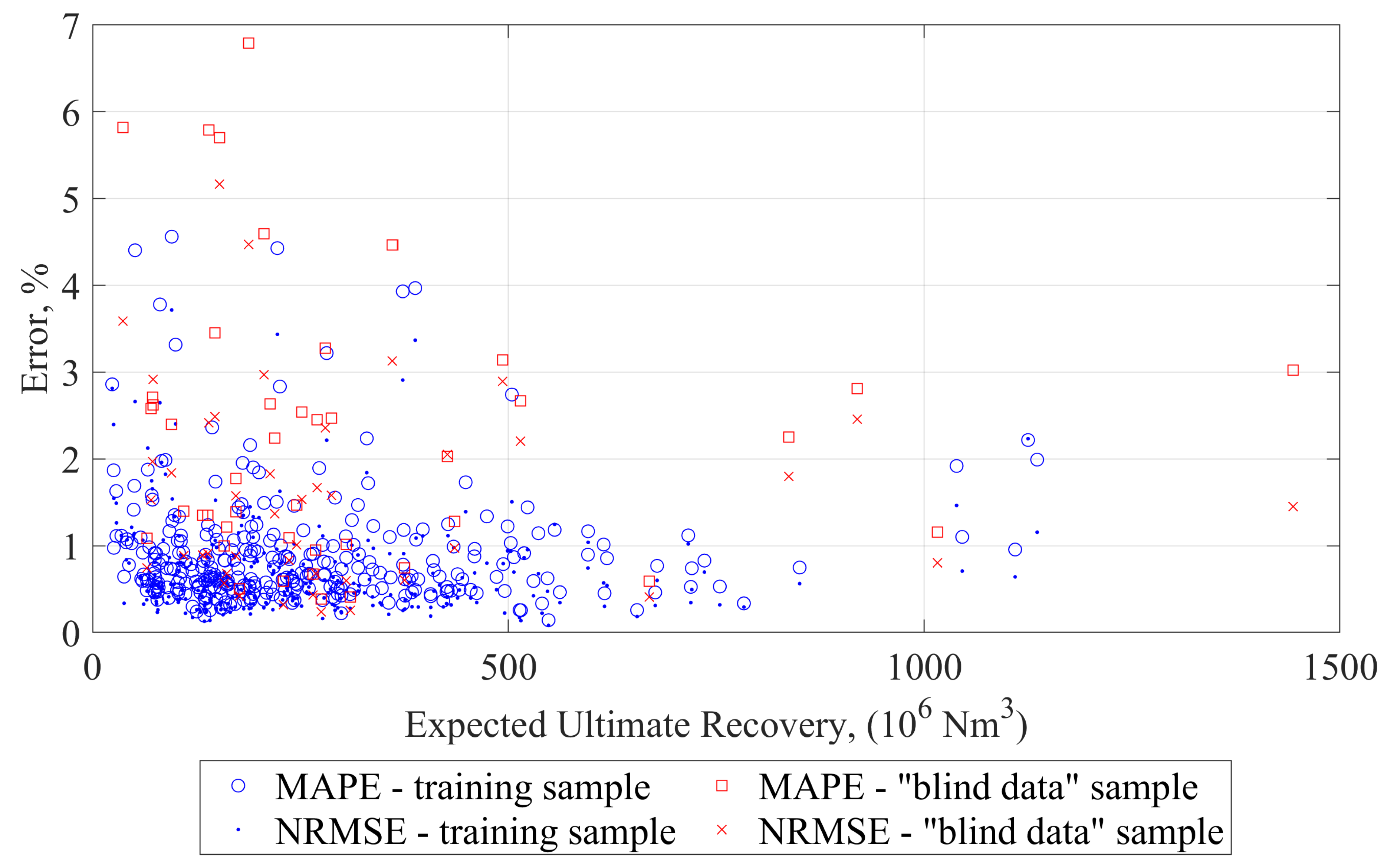
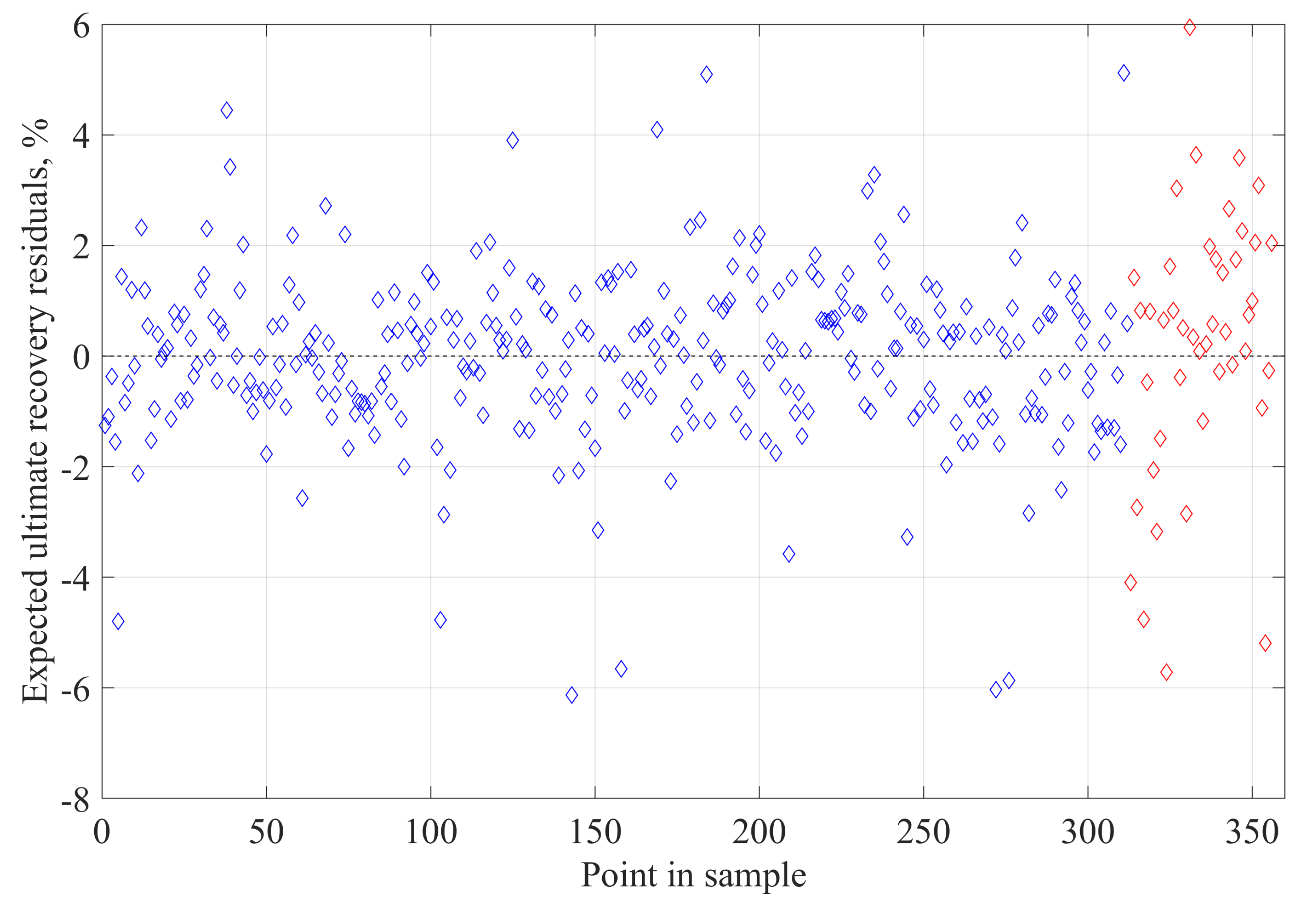
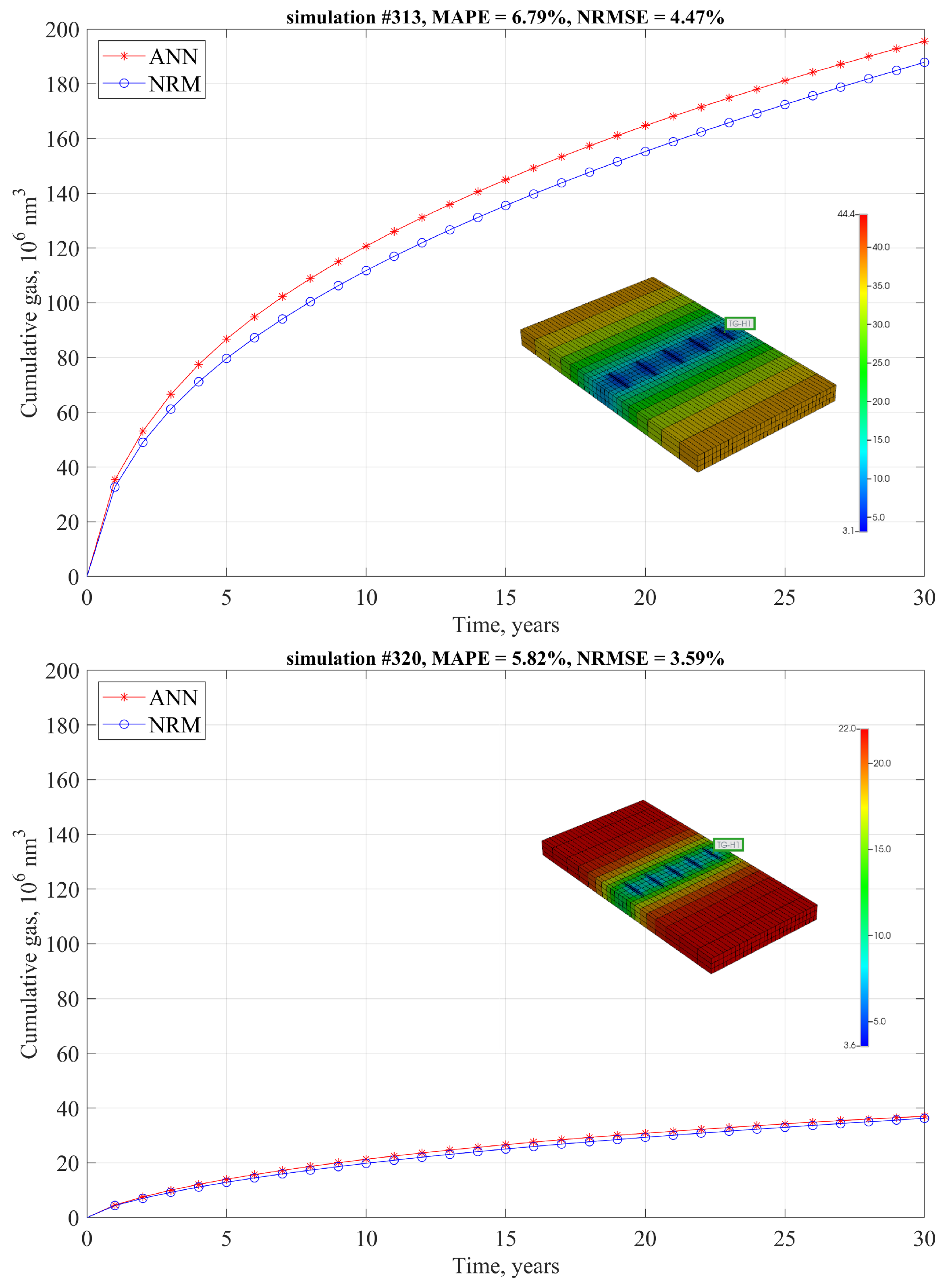
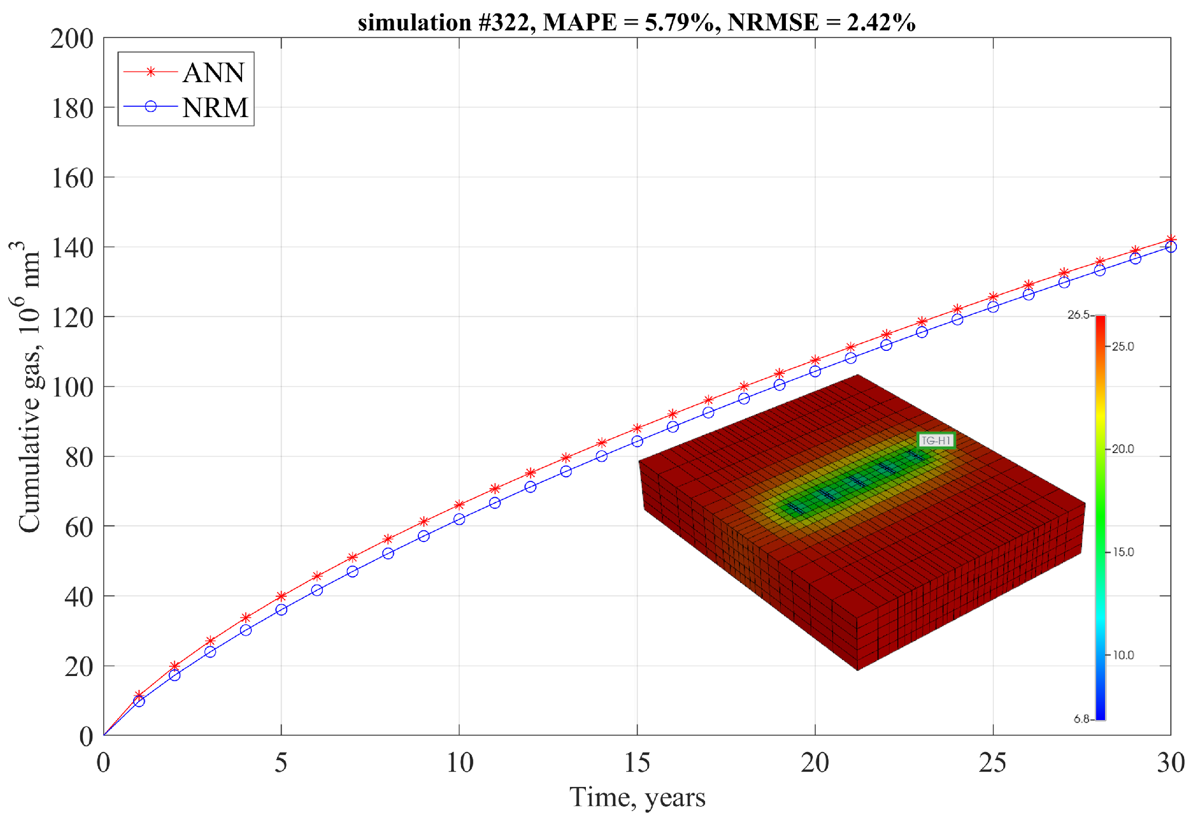
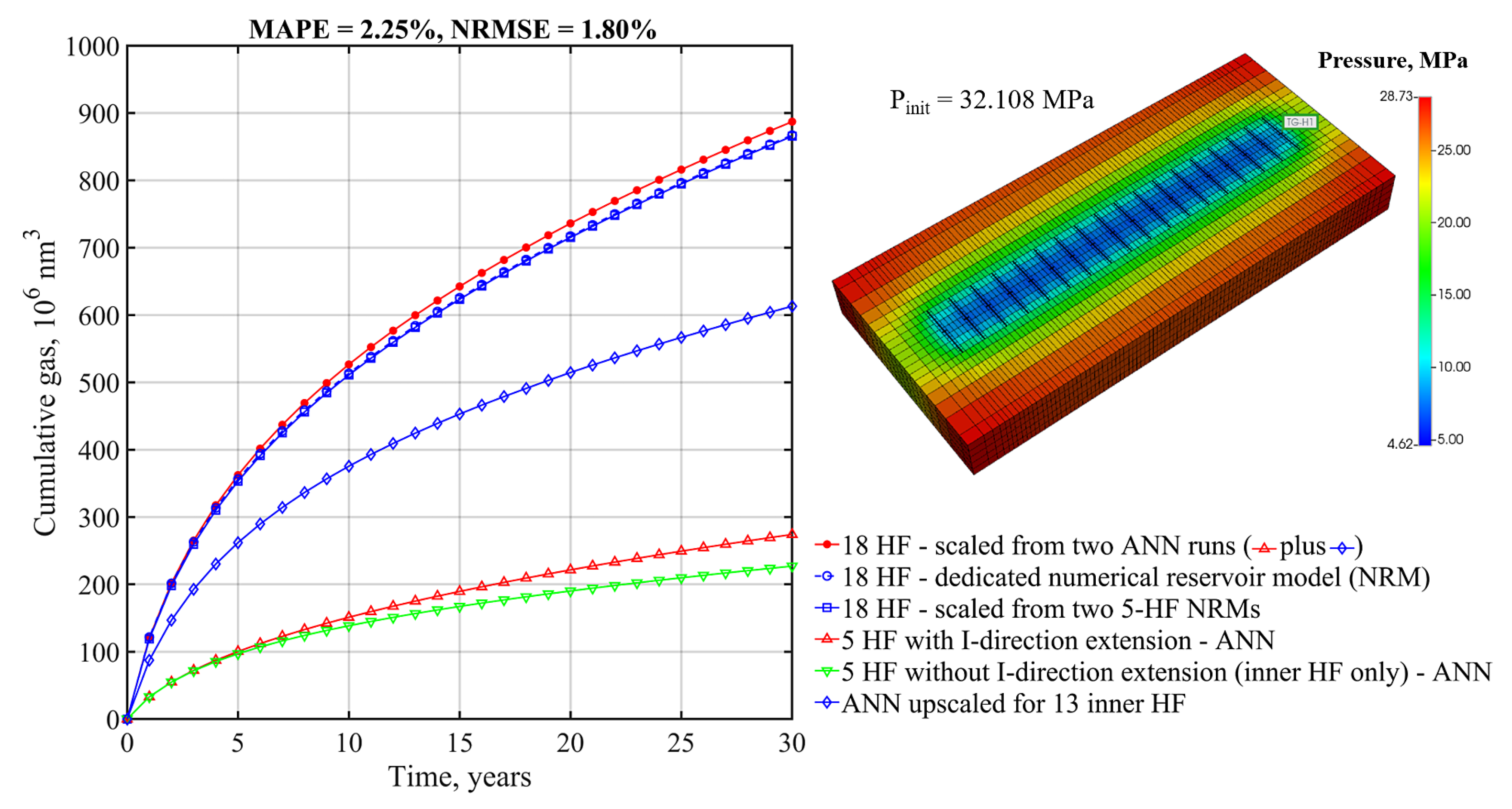
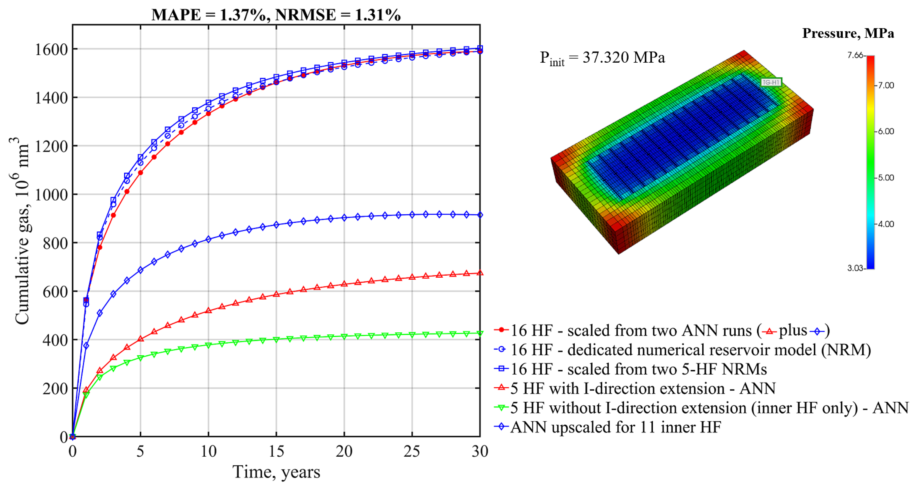
The developed method goes beyond the limitation of fixed “shoes box” models typically used in analyses of this kind and allows for dynamic analysis of the effects of parameters defining SRV as well as the external dimensions of the part of the reservoir being modeled. The simulation is extremely fast compared to numerical reservoir simulation. The performance of the developed model is examined using the mean average percentage error (MAPE) and normalized root mean square error (NRMSE) metrics, in addition to the simple metric of the Pearson correlation coefficient. Based on “blind data" only, MAPE and NRMSE is not greater than 4% for 86.4% and 95.5% of runs, respectively, and 79.5% of the EUR residuals is not greater than 2%. The upscaling procedure for the gas production profile was examined by comparison with dedicated numerical models for two different cases with 18 and 16 hydraulic fractures. The MAPE values of 2.25% and 1.37% and the NRMSE values of 1.80% and 1.31%, respectively, confirm that the ANN model agrees very well with the numerical models.

The process of developing the proposed tool and the essential conclusions can be summarized as follows.

• A high quality and cost effective database for tight gas production with multiple fractured horizontal wells is generated as the input for artificial neural network training and testing. The efforts incurred in creating the database pay off in the quality of the results. The database quality is achieved by (1) the comprehensive and reliable description of the reservoir and SRV and (2) the Latin hypercube sampling procedure optimized with the genetic algorithm that results in an optimized design representing the problem space of interest with a limited number of points.
• The Bayesian regularization backpropagation algorithm produces better results compared to the Levenberg–Marquardt backpropagation. The production profiles generated with networks trained with Bayesian regularization always increase smoothly.
• It is possible to effectively train the relatively small artificial neural network to mimic the behavior of the numerical reservoir model for unconventional tight gas reservoirs described by a set of key parameters with a relatively wide range of variability.
• The proposed method for upscaling the resulting production forecast for an increased (and limited only by practical issues) number of fractures proved to be useful and practical.

Taking into account the arguments presented, it can be concluded that the developed model may have practical applications in assessing the sensitivity and optimizing the development of tight gas reservoirs. Furthermore, the developed framework may be transferred/extended for problem spaces defined with different variability ranges/modified input parameters.