Abstract
For the advancement of smart grids, solar power generation predictions have become an important research topic. In the case of using traditional modeling methods, excessive computational costs may be incurred and it is difficult for these methods to learn the multi-variable dependencies of the data. Therefore, in this paper, a deep learning model was used to combine convolutional neural networks and long short-term memory recurrent network predictions. This method enables hourly power generation one day into the future. Convolutional neural networks are used to extract the features of multiple time series, while long short-term memory neural networks predict multivariate outcomes simultaneously. In order to obtain more accurate prediction results, we performed feature selection on meteorological features and combined the selected weather features to train the prediction model. We further distinguished sunny- and rainy-day models according to the predicted daily rainfall conditions. In the experiment, it was shown that the method of combining meteorological features further reduced the error. Finally, taking into account the differences in climate conditions between the northern and southern regions of Taiwan, the experimental results of case studies involving multiple regions were evaluated to verify the proposed method. The results showed that training combined with selected meteorological features can be widely used in regions with different climates in Taiwan.
1. Introduction
In recent decades, there has been a noticeable rise in the global energy demand, coinciding with a growing adoption of renewable energy sources in electrical grids worldwide due to climate change and environmental protection issues [1]. In order to comply with the world’s trend of using green energy, Taiwan has been increasing its proportion of green energy. Among all the sources of renewable energy, solar power generation is gradually becoming a major source of green energy in Taiwan. As the proportion of solar power generation increases, maintaining the stability of the power grid is an important issue [2]. The fluctuations in and intermittent characteristics of solar power generation are a big challenge to the stability of the power grid. In response to this challenge, energy management systems have arisen to address the complexities of grid management. Energy management systems play an important role in directing operational strategies within power grids, enabling the effective balancing of the energy supply and demand among distributed generators and consumers [3,4]. Among the technologies required in an energy management system, power generation predictions represent one of the crucial research topics [5]. Usually, the prediction of power generation can be performed on different time scales according to the demand of the power grid. For short-term predictions, the horizon of prediction ranges from 15 min to 1 h. For medium-term and long-term predictions, the prediction horizon ranges from a day to a week. Solar panel power generation data are essentially time series data. The fluctuations in the data are affected by seasonal changes and weather factors. The prediction methods can be mainly divided into statistical methods, traditional machine learning methods [6,7,8,9,10,11,12], neural network-based methods [13,14,15], and hybrid models.
Solar panel power generation data exhibits various characteristics. Essentially, it belongs to time series data, and its fluctuations are influenced by factors such as seasonal changes, weather conditions, and the time of day. Moreover, solar panel installations typically consist of multiple inverters, resulting in multiple sets of time series data for power generation simultaneously. These individual time series are subject to physical constraints of their respective inverters, leading to different upper and lower limits and variation cycles due to the positioning of solar panels. In previous studies, various methods have been used to address the challenges posed by multiple time series and weather factors. This chapter will briefly explain how different machine learning methods or deep learning methods have been optimized and utilized to handle the task of the multivariate prediction of power generation in both long-term and short-term prediction scenarios. This includes statistical methods, traditional machine learning methods, neural networks, and hybrid models.
The traditional statistical methods include the autoregressive integrated moving average (ARIMA) model [9], which is a univariate time series prediction method. However, it cannot learn long-term time patterns to cope with long-term prediction ranges. In machine learning methods, there are various models, such as support vector regression (SVR) [10], multiple linear regression (MLR) [11], and the Gaussian process (GP) [12]. These methods can deal with short-term prediction data and achieve multivariate time series predictions. However, they often incur high computational costs when dealing with a large number of time series. Therefore, modern approaches tend to use neural network methods, which are introduced below.
For neural network-based methods, the authors of [13,14,15] trained backpropagation neural networks with different sizes of time windows to deal with different prediction horizons. In modern studies, there have been important breakthroughs in feature learning for time series processing. Among them, convolutional neural networks (CNNs) [16] are used in feature extraction to extract time series features. The research in [17] proposed the use of a multi-layer CNN to deal with multi-variable input simultaneously and obtain predictions efficiently. Recurrent neural networks (RNNs) such as long short-term memory networks (LSTMs) [18] and gated recurrent units (GRUs) [19] can effectively achieve medium-term and long-term predictions. The system proposed in [20] used a bidirectional multi-layer RNN to train month-by-month data to cope with seasonal changes. The author of [11] tested different structures of RNNs, CNNs, and CNN–long short-term memory (CNN-LSTM) networks [21] for different prediction horizons. The research in [22] proposed LSTNet, which combined a Skip-RNN trained for periodic data and an RNN trained for general sequences. In addition, the authors added the results of the autoregression component simulated by MLP, allowing the model to learn short-term and long-term change patterns at the same time. The research in [23] proposed a multi-level construal neural network (MLCNN) to process data through multiple layers of CNNs. It extracted shallow and deep feature abstractions for multiple predictive tasks. The authors also combined the autoregressive model with a neural network to enhance the prediction performance.
In solar power generation, apart from selecting various methods for predicting with various time ranges, different data sources are also explored to be integrated into the prediction system. For example, ground-measured solar irradiance, sky images [24,25], and numerical weather predictions (NWPs) [26,27] can be applied. These data sources are utilized because solar power generation is closely related to weather factors. Whether it is seasonal changes or weather fluctuations, incorporating numerical weather prediction methods has a significant impact on medium- to long-term predictions. Approaches such as those used in [28,29] using a support vector machine (SVM) or LSTM combined with a k-nearest neighbors (k-NN) clustering analysis to identify similar weather data and train them separately to incorporate weather features have been proposed. Additionally, models such as a multi-layer RNN are introduced in [30], where various environmental features such as the module temperature, air temperature, relative humidity, wind speed, and solar irradiance are inputted together with power generation to predict the power generation one hour ahead.
The dataset used in this paper was collected from a solar power generation system with multiple inverters, so it was necessary to design a multivariable time series prediction model. This paper employed a multivariate time series prediction model to simultaneously predict data generated by multiple inverters in the power grid. Unlike traditional statistical regression or machine learning methods, which often involve large parameter counts and significant computational costs for multivariate predictions, this study constructed a deep learning model to predict the power output of multiple inverters simultaneously. Additionally, to address Taiwan’s diverse climate factors, this research combined weather features by training separate models for sunny and rainy weather types. Furthermore, historical data or numerical weather forecast data were integrated into the feature selection, along with training, to further enhance the accuracy. The aim was to develop a multivariate solar-power-generation prediction model that is applicable and effective for different regions and weather conditions in Taiwan. The model proposed in this paper combines numerical weather forecasting data and historical power generation data. It uses a two-dimensional convolutional network to learn the features of multiple time series to serve as the input of a GRU. Relevant weather features are concatenated to the feature vector to achieve better prediction results. The rest of this paper is organized as follows. Section 2 presents the system framework and research methodology, outlining the overall structure of the model and describing processes such as data collection, data cleaning, and preprocessing. The training and testing methods of the model in the experimental results are also explained in this section. Section 3 showcases the experimental results, including experiments with hyper-parameter selection, comparisons between the multivariate prediction results of weather features in different regions, and experiments comparing the results of different multivariate time series models. Finally, Section 4 concludes this paper and discusses future research directions.
2. Proposed Method
The proposed prediction framework and the dataset used for this research are elaborated upon in this section.
2.1. Data Acquisition
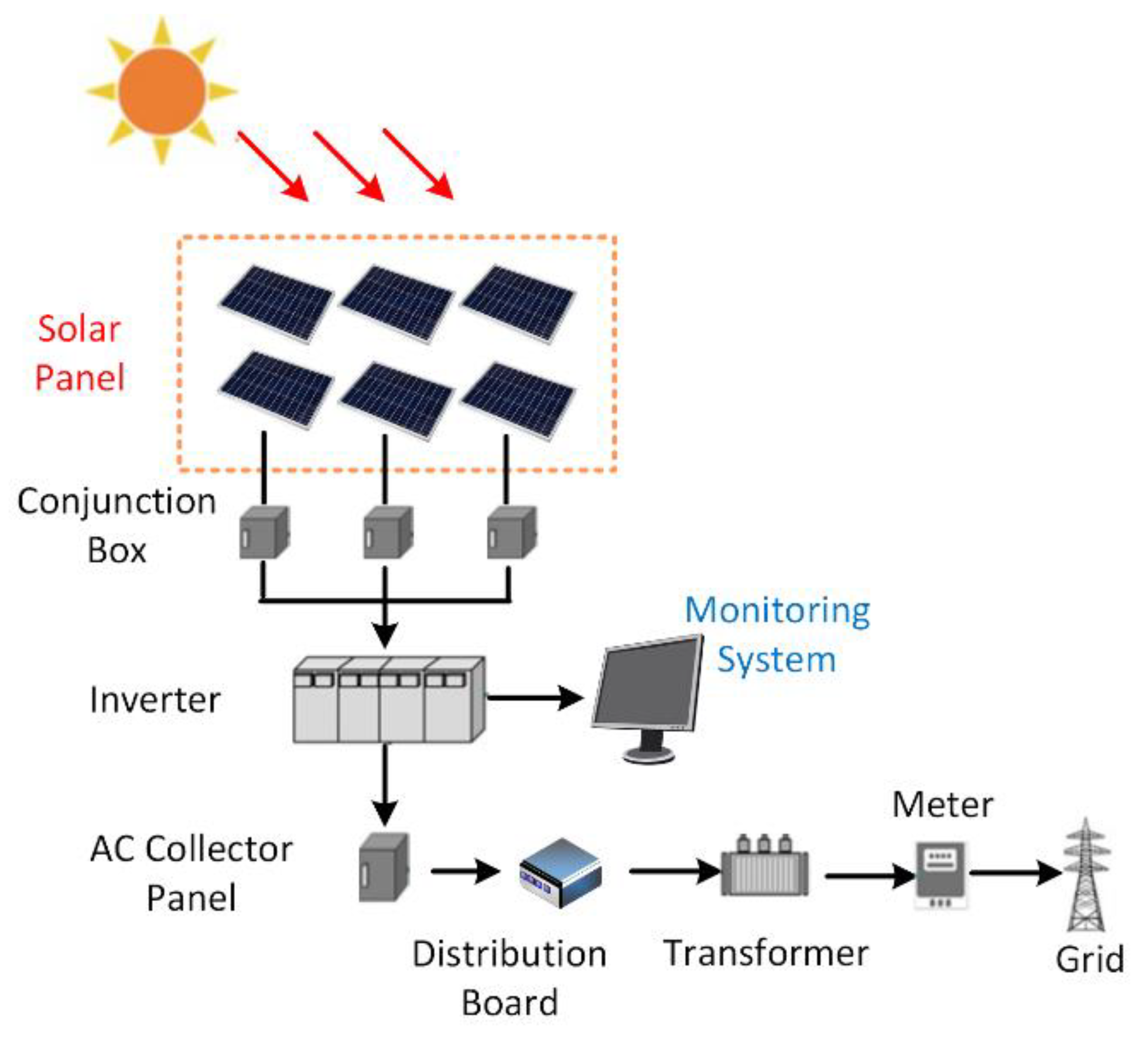
Figure 1 illustrates the modules in a solar power grid. The direct current (DC) power produced by multiple solar panels is converted into alternating current (AC) power by the inverters and enters the smart grid. The monitoring system records the current data of the inverter, which comprise an important indicator of power generation. As shown in Figure 1, there are usually multiple inverters in a solar panel factory, so multiple sets of time series data of power generation will be generated at the same time. Each time series will have different characteristics due to the physical limitations of its inverter and the location of the solar panel.

Figure 1.
Modules in a solar power grid.
The model training and testing utilized power data from solar panels provided for three sites by the Industrial Technology Research Institute (ITRI). All the datasets in this paper used the digital data in the inverter. The datasets were collected in different locations in Taiwan. These sites included Renhe Elementary School in Taoyuan, Liujia Campus in Tainan, and Fong-Da Technology in Taoyuan. Fong Da Technology provided data from three phases, totaling five datasets, extracted from the XML-format digital records of the solar panels at each site. We used the hourly power data of multiple inverters that started from 8:00 a.m. and ended at 6:00 p.m. Therefore, the number of data points in each day was 10. The unit of the power data is kilowatts.
The time periods for data collection and the amount of inverter power data varied across the five datasets, as shown in Table 1. Distinctions were made between multi-year datasets and single-year datasets in terms of the training and testing methods, specifically as follows:

Table 1.
Details of the dataset used in this paper.
- -
- The experiment at Renhe Campus in Taoyuan used multi-year datasets from 2015, 2017, 2018, and 2019. Each year included power data from 1 January to 31 December, with the data from two inverters provided.
- -
- The experiment at Liujia Campus in Tainan utilized power data from January to August 2019, with data from twenty inverters provided.
- -
- Fong-Da Technology in Taoyuan provided the following three datasets:
- Phase one, which covered power data from two inverters from January to August 2019.
- Phase two, which covered power data from two inverters from January to June 2019.
- Phase three, which covered power data from six inverters from January to August 2019.
All these datasets were used to validate and test the prediction of the hourly power output from multiple inverters one day ahead.
2.2. Proposed Prediction Framework
The proposed prediction framework is illustrated in Figure 2. To cope with multiple power time series generated by multiple inverters at the same time, we designed a model for multi-variable input and output. As illustrated in Figure 2, the proposed framework included several convolutional neural networks and a gated recurrent unit. The network is subsequently referred to as the multivariate convolution gated recurrent unit (MC-GRU) network. The inputs consisted of 10 × 1 hourly power data points at m inverters of D-1, D-2, and D-3 days. The CNNs served as the feature extractors. The feature maps generated by the CNNs were concatenated and reshaped to serve as the input for the GRU. Then, the output of the GRU was concatenated with the hourly power data of day (D-1) and the numerical weather data before passing on to a fully connected (FC) layer to produce the hourly power prediction of day D. The purpose of performing a concatenation with the hourly power data of day (D-1) was to emphasize the significance of the information from the previous day.
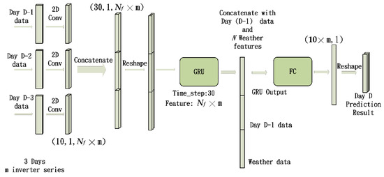
Figure 2.
Proposed system architecture.
The numerical weather data mentioned above includes the average temperature and relative humidity. We performed normalization on the values of the weather data. Then, the normalized weather features were concatenated to the feature vector before going to the fully connected layer. The dimensions of the feature vectors shown in Figure 2 are elaborated upon in Section 2.2.1. The loss function used to train the model was the standard mean squared error (MSE) in Equation (1). In Equation (1), denotes the predicted power, denotes the ground truth power at time instance t, and Ntr denotes the number of data samples used in the training dataset.
2.2.1. Convolution Layer
Convolutional neural networks are primarily used in neural networks for feature extraction. They can be applied to high-dimensional image data as well as single-dimensional time series data. In traditional architectures, CNNs are used to extract image features and are combined with fully connected layers for image classification tasks. In this study, we primarily utilized two-dimensional convolution. By sliding kernels over multiple time series datasets, we obtained features between the time and each sequence. Convolution operations were performed on local data using convolution kernels (also known as filters). Depending on the specified kernel size, the stride, and the number of kernels, different dimensional results were produced. The output results are referred to as feature maps. In our framework, to obtain features among multiple time series, we set the kernel size to cover all the time series features.
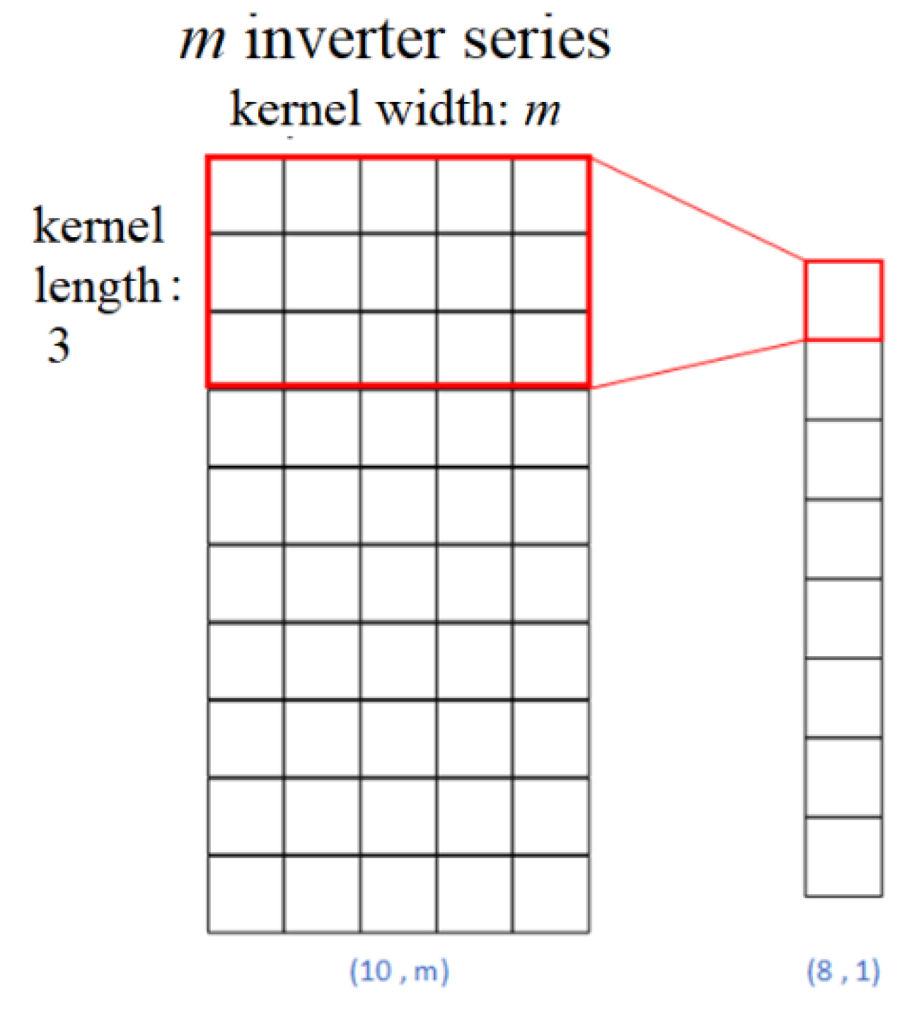
By changing the sizes of the kernels, the two-dimensional convolution operation can cover data at multiple time points and include multiple time series features at the same time. This design allows the CNNs to simultaneously extract relevant features of the multivariate time series. In Figure 2, m denotes the number of input inverter time series. The size of the 2D convolutional kernel was designed to be (Lk, m), where Lk is the length of the kernel and m is the width of the kernel. We can observe from Figure 3 that the kernels can completely cover m sequences to extract features. For the example illustrated in Figure 3, each 2D convolution operation with a kernel size (2, m) resulted in an (8, 1) feature map. Since the inputs were 10 × 1 hourly power data points at m inverters, zero padding was performed to bring the dimension of the output feature map of the 2D convolution back to (10, 1). Supposing that there are Nf kernels, the dimensions of the output of the 2D convolution would be (10, 1, Nf ). After 2D convolution, the system concatenated the feature vectors of three days to form a feature map of (30, 1, Nf ). Then, the feature map was reshaped to serve as the input of the GRU. The timestep of GRU was 30, and the number of features was Nf . The output of GRU had a size of (Nf , 1). The dimension of the output of the fully connected layer was (10 , 1), which matched the dimension of the 10 h of the predicted hourly power value at m inverters.

Figure 3.
Process of 2D convolution on multiple time series.
2.2.2. Pooling Layer
In some architectures, using pooling layers can reduce the number of trainable parameters and improve the performance. The commonly used pooling methods are max pooling and average pooling. Pooling on two-dimensional feature maps reduces the convolution output and retains important features. In max pooling, the output is updated to the maximum value within the pooling kernel, while average pooling updates it to the average value within the pooling kernel.
2.2.3. Fully Connected Layer
In classical convolutional neural networks, fully connected layers typically reside at the end, after the feature extraction step. In fully connected layers, each neuron in the layer is connected to every neuron in the preceding layer. This means that every output from the previous convolutional or pooling layer is connected to every neuron in the fully connected layer. This is used to interpret the features extracted by earlier layers. Fully connected layers consist of many neurons and are commonly used as classifiers in classical architectures. In essence, the fully connected layer helps the CNN make sense of the high-level features extracted by the convolutional layers and make predictions based on these features. In multivariate models, fully connected layers can integrate prediction features from multidimensional time series and map out the dimensions of time series that need to be simultaneously predicted, thus aggregating the final prediction results for the output.
2.2.4. Gated Recurrent Unit (GRU)
RNNs such as LSTMs and GRUs are suitable for capturing relationships among sequential data types. The primary distinction between GRUs and LSTMs lies in their management of the memory cell state. In LSTMs, this state is kept distinct from the hidden state and undergoes updates through three gates: the input gate, the output gate, and the forget gate. Conversely, GRUs replace the memory cell state with a candidate activation vector, modified via two gates: the reset gate and the update gate. The reset gate regulates the degree to which the previous hidden state is disregarded, while the update gate regulates how much of the candidate activation vector influences the new hidden state. Similar to other recurrent neural network designs, GRUs process sequential data step by step, adjusting their hidden state based on the current input and preceding hidden state. At each time step, they compute a candidate activation vector combining information from the input and prior hidden state. This vector then updates the hidden state for the subsequent time step.
Reducing the number of gates can decrease the number of parameters and improve the training speed. Also, it can sometimes result in a better performance on smaller datasets. In addition, GRUs eliminate the cell state for their output. The design of the GRU structure allows it to dynamically capture dependencies within time sequences while retaining information from earlier segments of the sequence. Therefore, GRUs stand as a popular alternative to LSTMs for sequential data modeling, particularly in scenarios where computational resources are constrained or a simpler architecture is preferred.
The following is a brief description of the process of GRUs [19]. The GRU model is presented in the form of Equations (2) and (3).
In Equations (2) and (3), the operation ☉ denotes element-wise multiplication. denotes the candidate activation vector. The computation of the candidate activation vector involves two gates. The reset gate , determines the extent of the memory to discard from the prior hidden state. The update gate governs how much of the candidate activation vector influences the new hidden state. In Equation (3), is the activation function. It is typically a hyperbolic tangent function, as shown in Equation (4).
The update gate and reset gate are defined as Equations (5) and (6). These gates are responsible for controlling the information to be kept or discarded at every time step.
The update gate is computed using the previous hidden state and input data at the current time instance. The previous hidden state and current input are multiplied with their weight matrices, respectively. The results are summed and passed through a sigmoid function .
The reset gate is also calculated using both the previous hidden state and the current input data . Both the update gate and the reset gate have similar formulas. However, the weights multiplied with the input and hidden state are specific to every gate. Therefore, the output vectors for every gate are different. The function in Equations (5) and (6) is a sigmoid whose output range is [0, 1], as defined in Equation (7). The sigmoid function transforms the values within the range of [0, 1] so that the gate can filter out the irrelevant information and retain only the important information in the subsequent steps.
In the above equations, the weight matrices , , , , , and the bias vectors , , are to be learned during the training process. The output layer of the GRU accepts the last hidden state as the input and generates the output of the network. This output may be a single number, a sequence of numbers, or a probability distribution across classes, depending on the specific task being addressed.
2.3. Training and Testing Procedures
The weather observations and forecast data from the prediction day were used in the training and prediction processes. The weather observations and forecasted information were obtained from the Central Weather Bureau, Taiwan. The observed values were used during the training phase. The forecast values were used during the prediction phase. More specifically, the power prediction model was trained from the historical power data and weather measurement features. During the prediction phase, the inputs of the trained prediction network were the power data of the previous days and the weather forecast data of the prediction day.
In addition to concatenating the weather features before the fully connected layer, we constructed separate models based on the rainfall weather parameter. Two models, the rainy model and the normal model, were trained using data for different types of weather. During the training process, if the measured total rainfall on the day to be predicted was lower than a certain threshold, the data were utilized to train the normal model. Otherwise, the data were utilized to train the rainy model. During the prediction phase, if the forecasted rainfall probability for the day to be predicted fell below a certain threshold, then the normal model was applied to obtain the prediction. Otherwise, the rainy model was used.
The amount of data required to train the proposed multivariate convolution gated recurrent unit network was relatively small. The proposed prediction model can be successfully trained using data within the duration of one month. We adopted the sliding window training mechanism suggested in [21] in the training process. More specifically, when predicting the power data in August, the data collected in July were used to train the MC-GRU model. And the data in June were utilized as the validation set in order to determine the number of epochs to prevent overfitting. Models trained by the sliding window training mechanism were better able to adapt to seasonal changes. This sliding window training mechanism also helped with fast deployment when the data collected from a specific site were limited in the initial deployment phase.
2.4. Data Preprocessing
The original inverter data provided by ITRI were in XML format and needed to be parsed and converted. Additionally, the recorded data intervals varied across different regions, with intervals of 10 s, 30 s, or one minute. Therefore, the data needed to be resampled, and the samples needed to be averaged to organize them into hourly power data. The organized data were then combined with the observed and forecasted weather data, both recorded hourly. Within this combined dataset, there may be invalid values generated during periods when the observation stations were inactive. To address this, the method of filling invalid data with the last valid data point was employed. Finally, only the effective photovoltaic generation period within a day, from 08:00 to 18:00, was selected as the hourly dataset required for the experiment. All the data were normalized when inputted into the model, thus mapping the data into the [0, 1] range. And the value of the data was restored during validation and testing.
3. Experimental Results
The experimental results are reported in this section. In our experiments, the Adam optimizer [31] was used to perform the training. We used 0.001 as the initial learning rate. In the training process, the reduction in the error was assessed every 40 epochs. If the reduction in error did not exceed a certain threshold, the new learning rate was set as 0.6 multiplied by the original learning rate. The best number of epochs was determined by the validation dataset. A maximum number of 350 epochs was set.
We used the mean absolute percentage error (MAPE) to evaluate the prediction accuracy of the proposed model. The definition of the MAPE is shown in Equation (8). In Equation (8), Num denotes the number of data samples used in the testing dataset. The mean absolute percentage error measures the absolute difference between the predicted power and the ground truth power at time instance t in terms of percentage in contrast to the ground truth values.
3.1. Selection and Combination of Weather Features
In the selection and combination of weather features, we employed two methods of integration: combining highly correlated features during training and utilizing a sunny–rainy-day model based on the rainfall amounts corresponding to different weather conditions. Within the weather features, we utilized features present in both the historical observed weather data and the numerical weather data, including the relative humidity (RH), temperature (Temp), wind speed (WS), and wind direction (WD), for feature selection. We calculated the Pearson correlation coefficient (Pearson’s R) between each weather feature and inverter power. The formula for the calculation, as shown in Equation (9), involves the covariance between two features divided by the product of their standard deviations, with X and Y representing the two features being correlated and and representing the mean values of the two features. The resulting correlation coefficient ranged from -1 to 1, where positive values indicate positive correlations and negative values indicate negative correlations. We used the dataset from Taoyuan Renhe to perform this experiment. The final calculated results, represented in Table 2, displayed the correlation coefficient matrix in percentage form. Among them, higher correlation coefficients were observed for the positive correlation of temperature features and the negative correlation of relative humidity features. Consequently, the experiments compared the results using these two weather feature combinations. Additionally, weather features from different times, such as the last training day and the day of prediction, were utilized for selection.

Table 2.
Correlation coefficient matrix of weather features.
In addition to selecting weather features, we also categorized the dataset using weather conditions based on the daily rainfall amounts. We summed the rainfall amounts for the 10 h peak electricity-generation period of each day to classify the weather conditions. If the sum was 0, it was classified as sunny; otherwise, it was classified as rainy. To verify the effectiveness of training under different weather conditions, we used data from Renhe Elementary School and analyzed the data when categorizing different weather conditions, as shown in Table 3. The dataset was divided into different weather conditions, with the unbiased variance calculated for the 10 h period from 8:00 to 18:00. In the original dataset without classification, the hourly variance was higher, indicating greater data fluctuation. However, for the datasets classified as sunny and rainy weather, the hourly variance was reduced, making the model easier to fit the data.

Table 3.
Unbiased variance in hourly inverter power dataset under each weather condition.
3.2. Experiment on Convolutional Data Padding
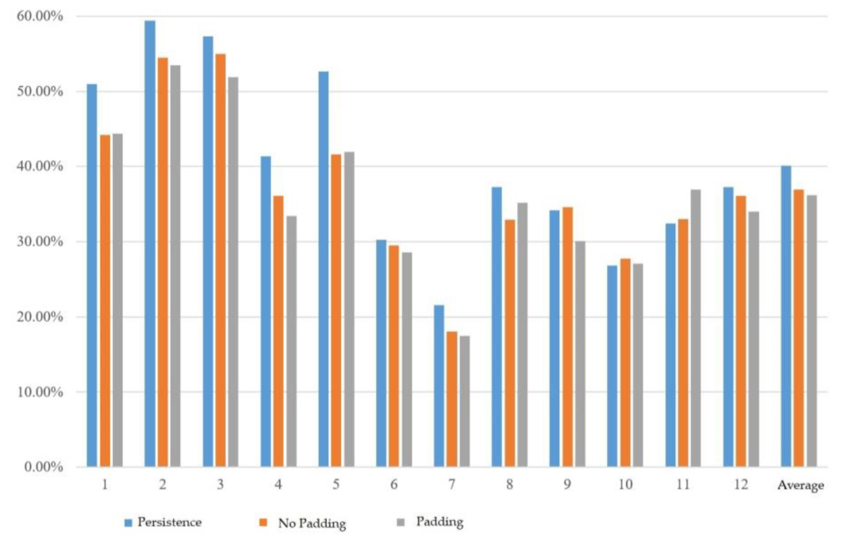
We first tested convolutional data padding. In this experiment, the convolutional kernel length was fixed at 3 and no pooling layer was used. The experimental results displayed the mean absolute percentage error (MAPE) for each month from January to December, and then calculated the average. As shown in Figure 4, the MAPE without convolutional data padding was 36.94%, while the MAPE with convolutional data padding was 36.20%. The error was lower when the data padding was applied. Therefore, for subsequent experiments, convolution with data padding was used as the default setting.

Figure 4.
Experimental results of convolutional data padding.
3.3. Experiment on Using Pooling Layers and Convolutional Kernel Length
As shown in Table 4, the results indicated that using pooling layers did not significantly reduce the MAPE, and the best performance was achieved when using a convolutional kernel length of 5 without pooling layers. Therefore, no pooling layers were used in subsequent experiments.

Table 4.
MAPE of using different pooling layers and convolutional kernel lengths.
3.4. Experiment on the Number of Convolutional Kernels
We can observe from Table 5 that the best performance was achieved when there were 10 convolutional kernels. The errors were higher when there were slightly more or fewer kernels. Even with a significant increase in the number of convolutional kernels, the error could not be reduced. Therefore, in subsequent experiments, 10 was used as the number of convolutional kernels.

Table 5.
MAPE when using different numbers of convolutional kernels.
3.5. Experiment on the Integration of Weather Features at Each Site
The experiments are represented by different codes, as shown in the following list.
- -
- Combining temperature features from the last training day: T;
- -
- Combining temperature features from the prediction day: pT;
- -
- Combining relative humidity features from the last training day: R;
- -
- Combining relative humidity features from the prediction day: pR;
- -
- Combining temperature and relative humidity features from the last training day: RT;
- -
- Combining temperature and relative humidity features from the prediction day: pRpT.
3.5.1. Data from TaoYuan Renhe Elementary School
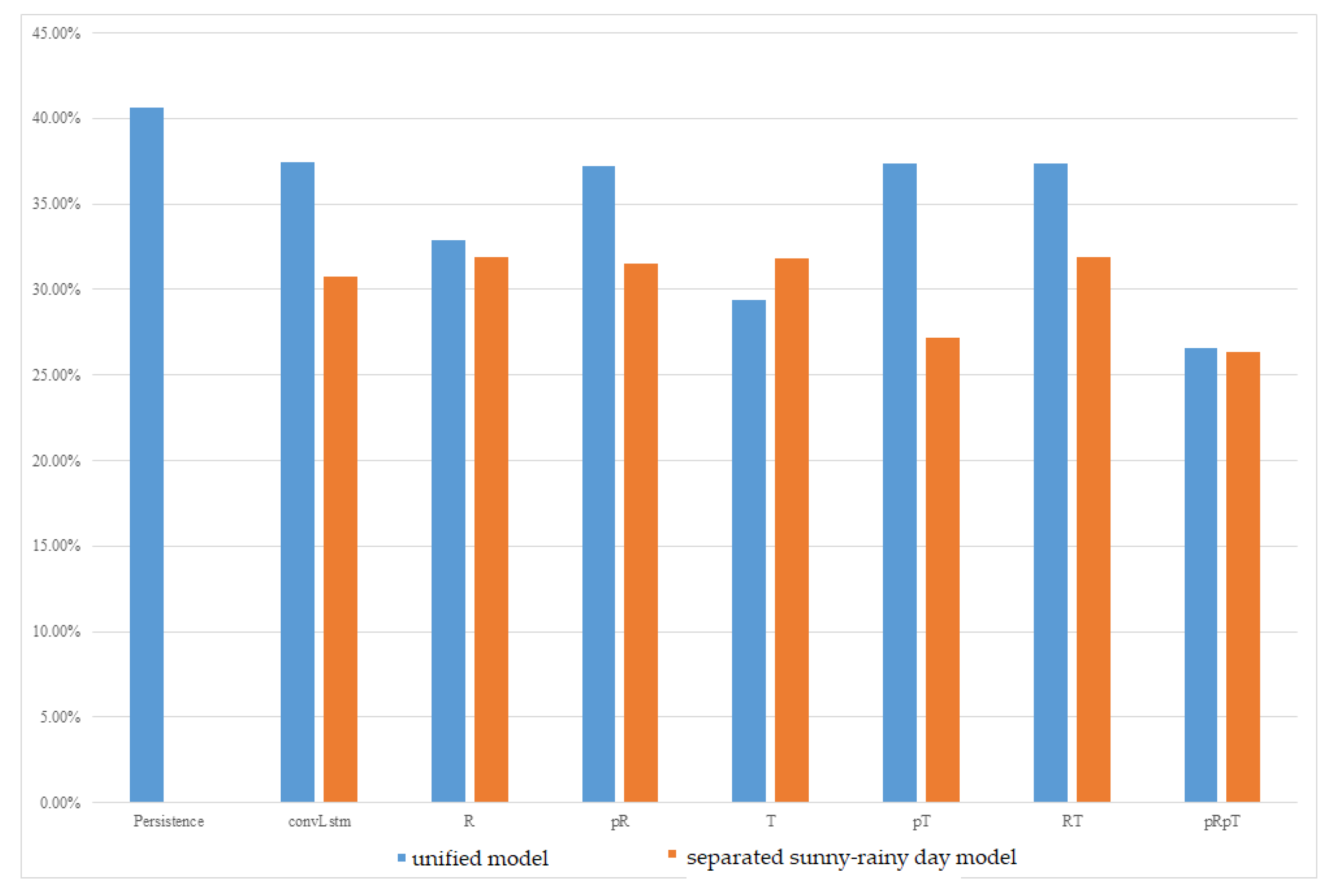
The experimental results of the MC-GRU one-day-ahead power prediction using the data collected at the Taoyuan Renhe Elementary School are shown in Figure 5. In Figure 5, the vertical axis displays the MAPE for all the months, while the horizontal axis shows different weather feature usage scenarios. It can be observed that, in the Renhe Elementary School area of Taoyuan, the separation of the sunny–rainy-day MC-GRU models can effectively reduce errors. In the experiments, combining forecasted weather features performed better than using data from the last day of training across different combinations of weather features. However, the model that considered relative humidity alone was less stable and showed less improvement. The best combination was the sunny–rainy-day MC-GRU model with pRpT. Combining the temperature and relative humidity of the prediction day helped further reduce errors in the sunny–rainy-day MC-GRU model. Compared to the persistence model, with a 40% MAPE, the proposed MC-GRU pRpT model exhibited an obvious improvement. According to Figure 5, the proposed MC-GRU pRpT model also outperformed the convLstm model proposed in [21].

Figure 5.
MAPE of one-day-ahead multivariate prediction models at Taoyuan Renhe Elementary School.
3.5.2. Data from Tainan Liujia
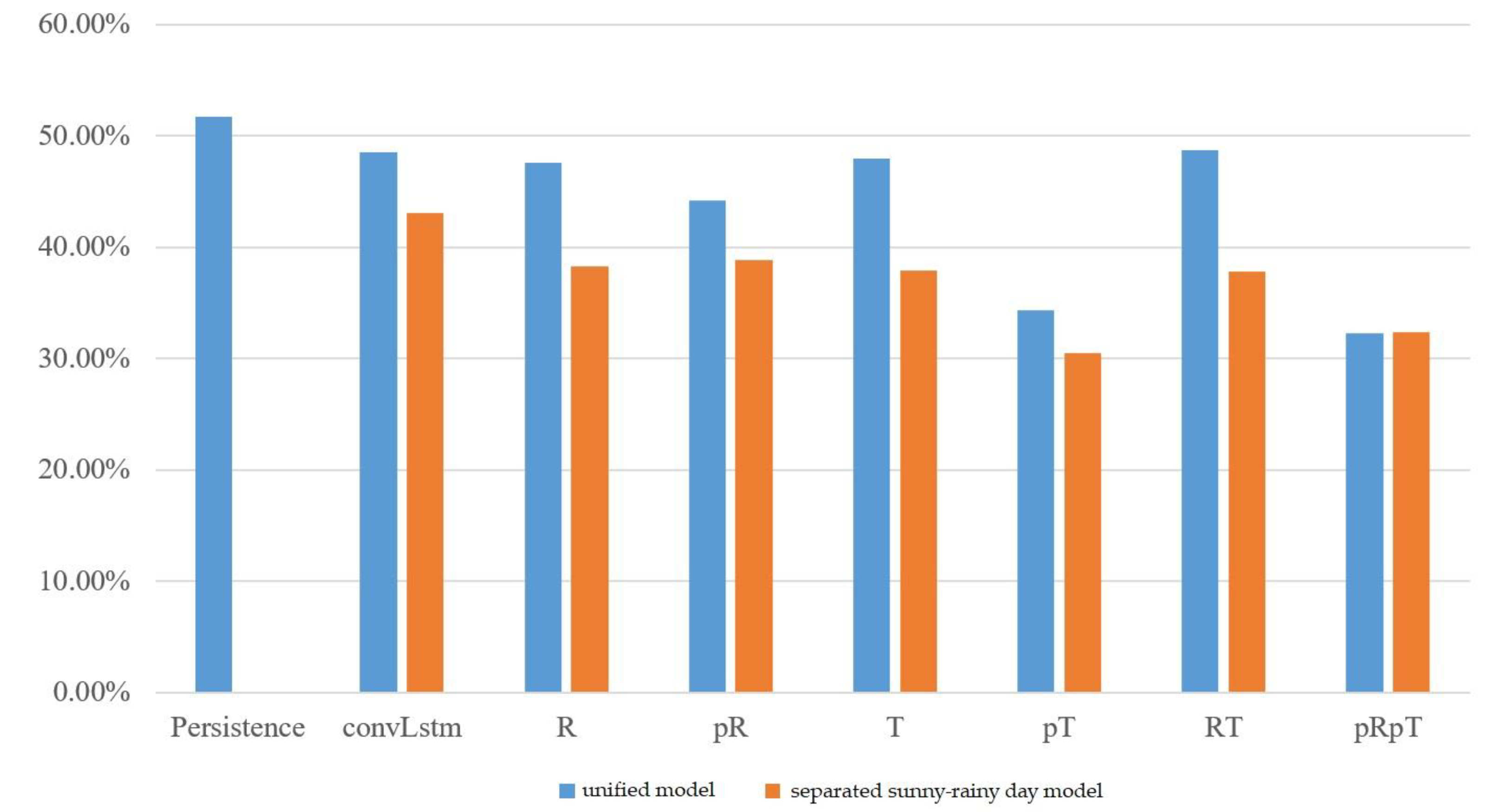
The experimental results of the MC-GRU one-day-ahead power prediction in Tainan Liujia are shown in Figure 6. In this dataset, there was very little rainy data because it seldom rains during this period in Tainan. The amount of data was also relatively small in this dataset. It only consisted of 6 months of data (from March to August). The rainy-day model could not be well trained due to a lack of sufficient data, and therefore, it tended to produce unstable predictions. As a result, separated sunny–rainy-day MC-GRU models are unable to consistently reduce errors. Therefore, a unified model tends to achieve better prediction accuracy than separated sunny–rainy-day models. Among all the meteorological features considered, the unified model combined with pT or pRpT consistently reduced prediction errors. It achieved a better MAPE compared with the persistence model and the convLstm model proposed in [21] across up to 20 inverter sequence predictions.
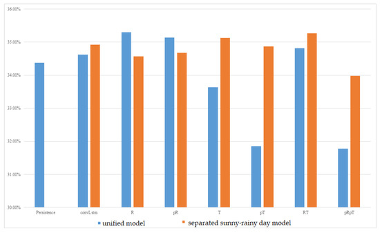
Figure 6.
MAPE of one-day-ahead multivariate prediction models at Tainan Liujia.
3.5.3. Taoyuan Fong-Da Technology
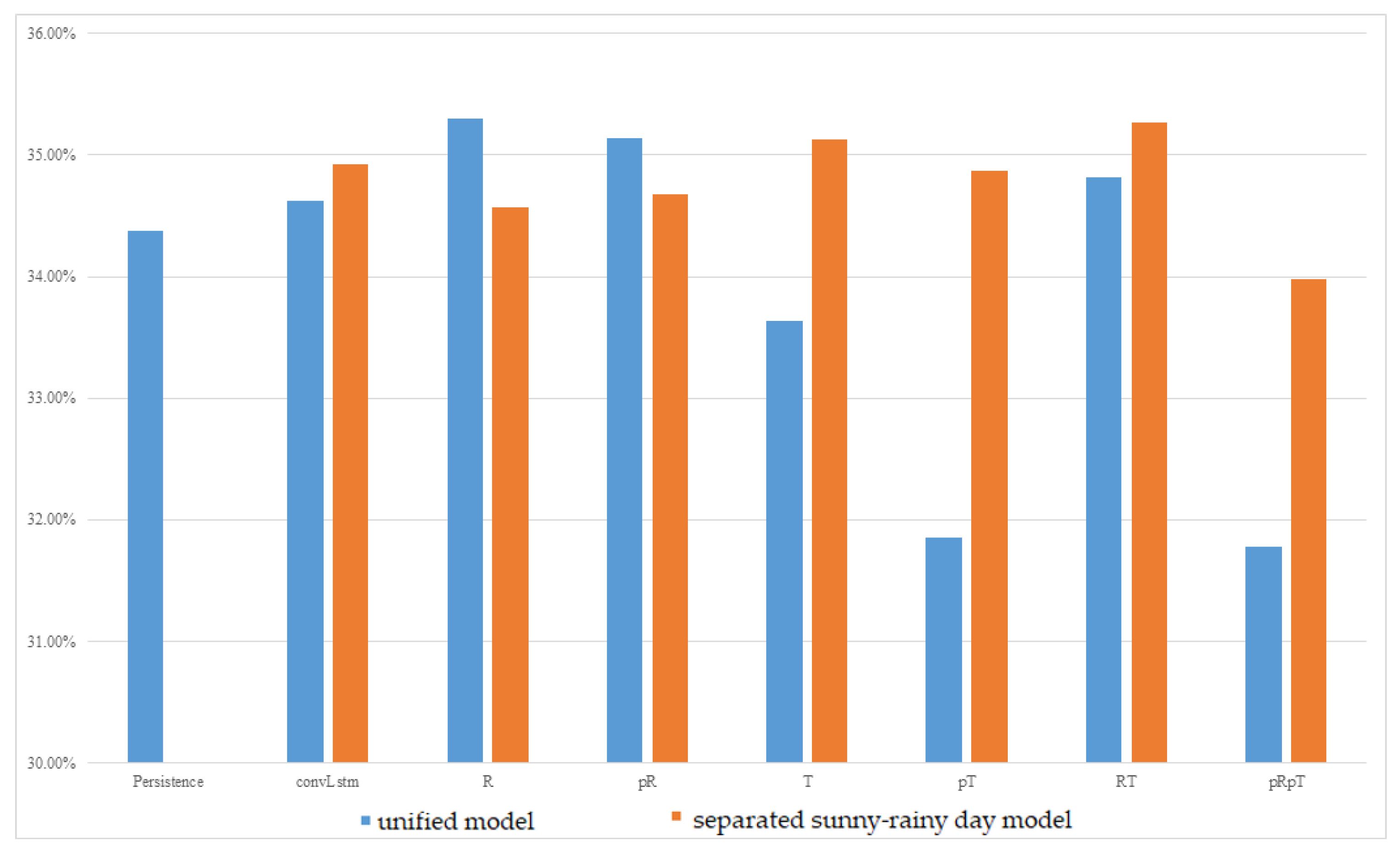
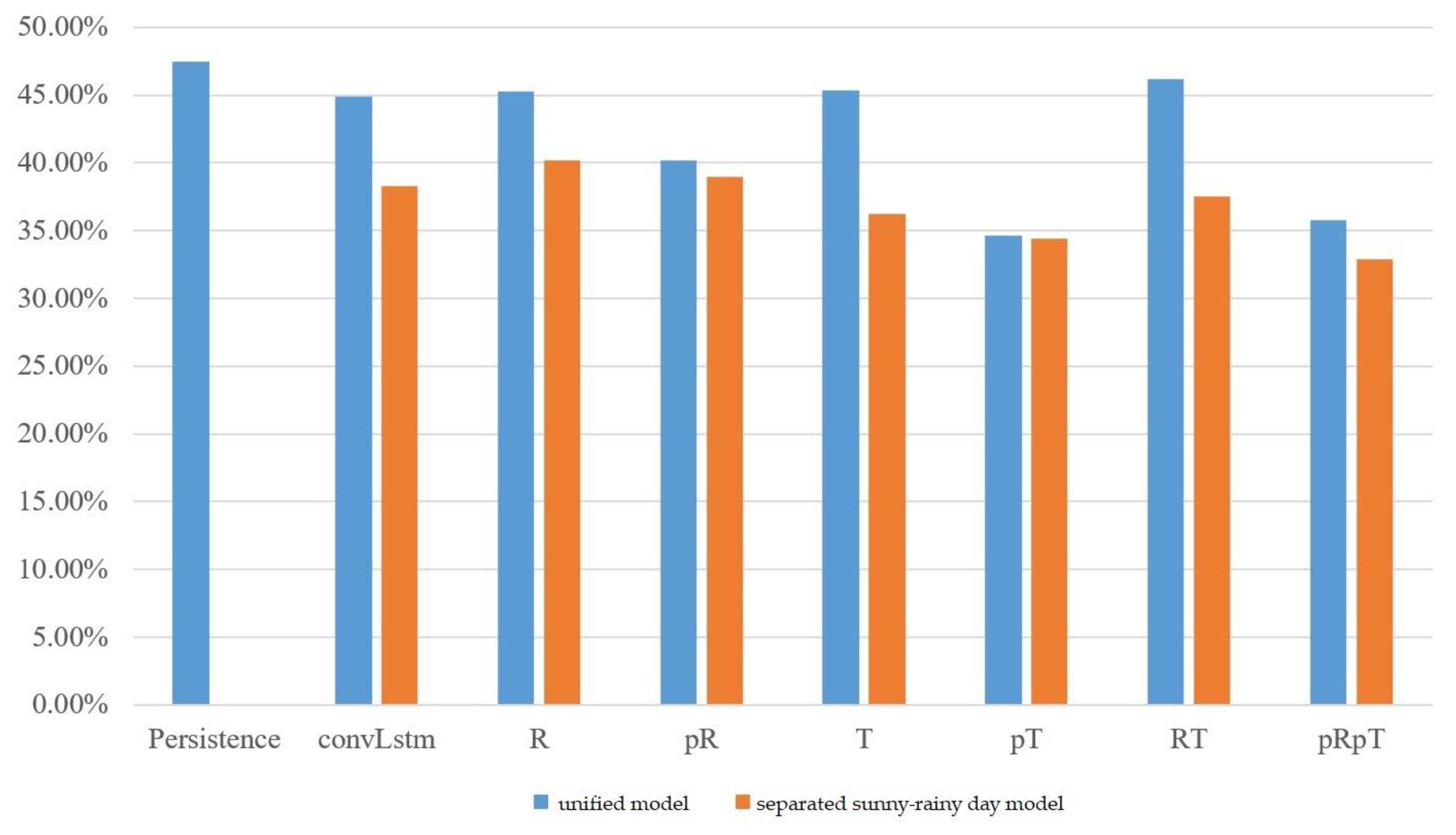
The experimental results of the MC-GRU one-day-ahead power prediction in Taoyuan Fong-Da Technology, phases one, two, and three, are shown in Figure 7, Figure 8, and Figure 9, respectively. We still observed that the separated sunny–rainy-day MC-GRU models can significantly reduce errors. The best prediction results were achieved when the separated sunny–rainy-day MC-GRU models were combined with pT or pRpT. Compared with the persistence model and the convLstm model proposed in [21], the proposed pT or pRpT models can substantially reduce the prediction MAPE.
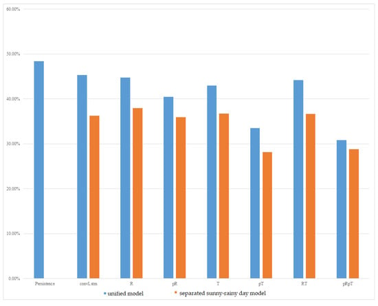
Figure 7.
MAPE of one-day-ahead multivariate prediction models at Taoyuan Fong-Da Technology, phase one.

Figure 8.
MAPE of one-day-ahead multivariate prediction models at Taoyuan Fong-Da Technology, phase two.

Figure 9.
MAPE of one-day-ahead multivariate prediction models at Taoyuan Fong-Da Technology, phase three.
3.6. Comparisons with Existing Works
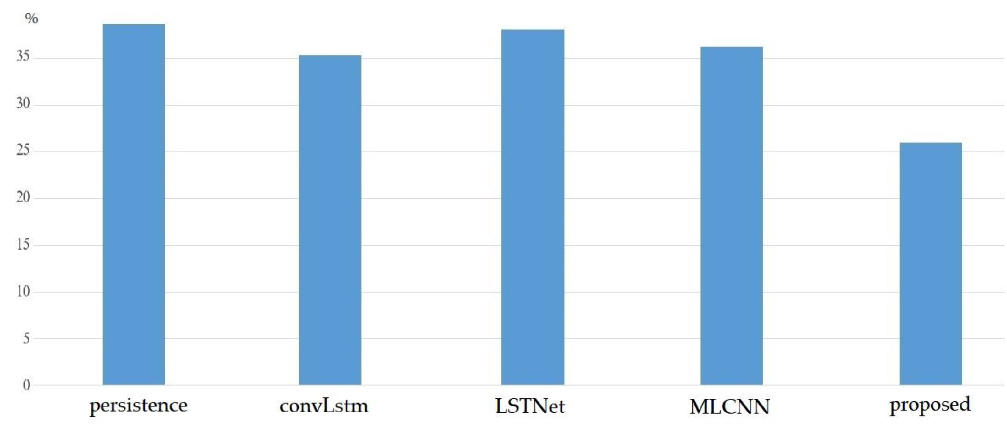
Figure 10 summarizes the comparisons of the MAPE of the proposed works and existing models, including the persistence model, the convLstm model proposed in [21], the LSTNet model proposed in [22], and the MLCNN model proposed in [23]. We observed that the proposed method exhibited the lowest MAPE compared with these existing methods.
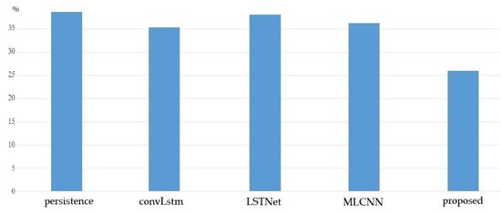
Figure 10.
Comparisons of MAPE with existing works.
3.7. Visualization of Prediction Results
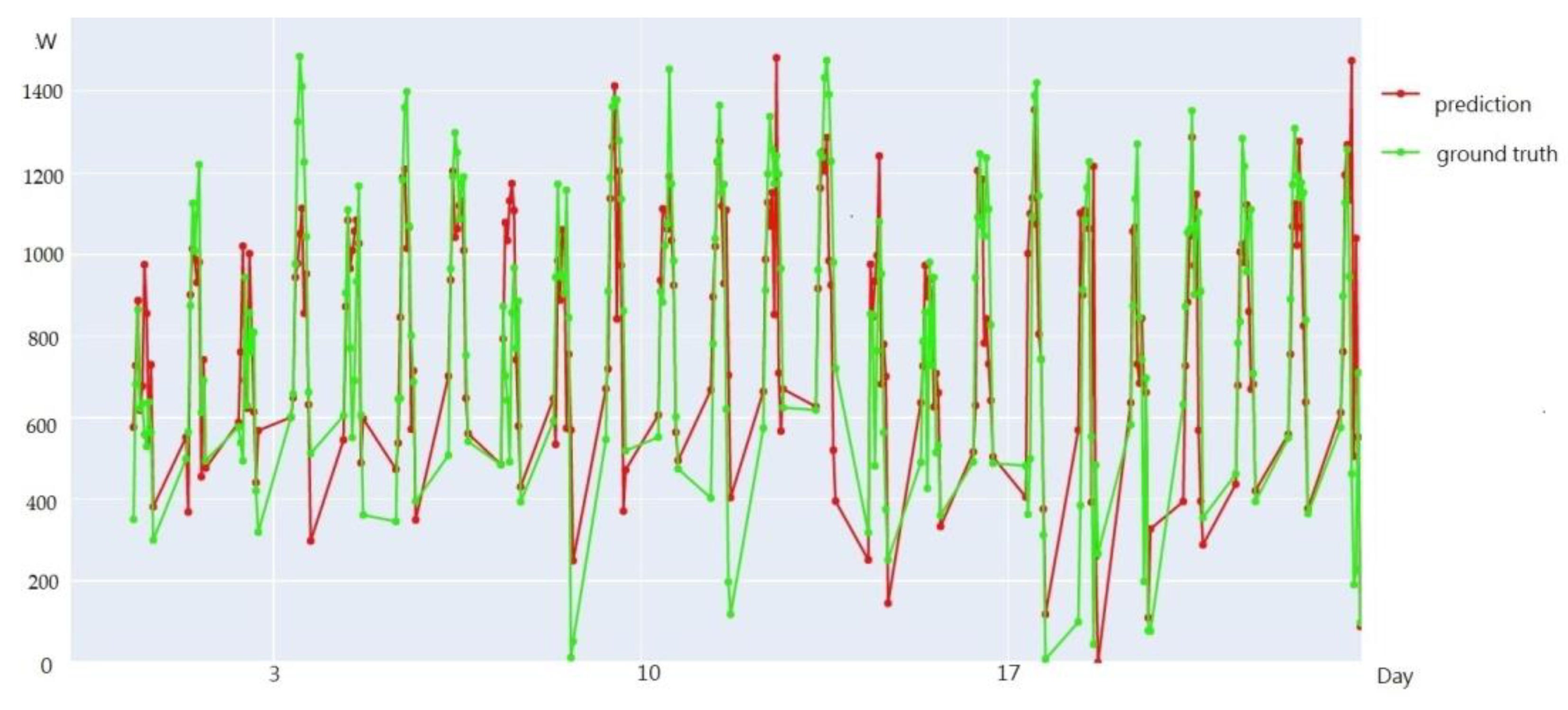
An example of the visualization of the prediction results for Taoyuan Renhe during 24 days in July, 2019, is shown in Figure 11. In Figure 11, the green line represents the ground truth values, while the red line represents the predicted values. As shown in the visualization figure, when training was completed using the weather model integration approach proposed in this paper, most of the predicted data fit the ground truth values well, demonstrating a good prediction performance.
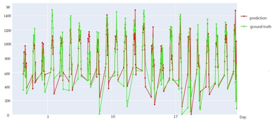
Figure 11.
An example of the visualization of the prediction results for Taoyuan Renhe during 24 days in July.
3.8. Discussion
In the dataset belonging to the Taoyuan area in northern Taiwan, which included data from Renhe Elementary School and the Fengda Technology phase one to three datasets, the sunny–rainy-day MC-GRU models exhibited the lower errors compared with the unified model trained using data for all weather. In most of the experiments, the combination of the sunny–rainy-day MC-GRU with pT or pRpT was the most stable and effective weather feature combination. In some cases, adding both relative humidity and temperature information was slightly better than adding temperature alone. However, in other situations, it was the opposite. Nevertheless, the difference between the two options was not significant. Therefore, choosing either the pT or pRpT model will do. For simplicity, pT would be a good choice, since it requires only temperature information. In the Lujia Campus area of Tainan, which resides in the southern part of Taiwan, the unified model was more stable in most combinations due to the scarcity of rainy-day data. The sunny–rainy-day model might result in significantly increased errors due to difficulties with fitting. As a result, in areas with less rainfall, it is preferable to use the unified model trained by data for all weather. In such areas with less rainfall, the combination with temperature features can still effectively reduce the prediction errors. In other words, the pT model would result in a preferable accuracy. In summary, the most widely used combination of weather features is the use of the daily temperature, which can achieve a stable prediction accuracy in both the northern and southern regions. The suggested weather condition model to be used in the northern regions is the sunny–rainy-day model. In the southern regions, we suggest that the all-weather model should be used.
4. Conclusions
This study proposed a multivariate electricity-generation prediction model capable of simultaneously predicting multiple time series. By combining convolutional neural networks with gated recurrent unit models, the model utilized two-dimensional convolution to extract data features from multiple time series electricity datasets and employed a GRU for multiparameter prediction. In the proposed framework, a GRU was selected instead of an LSTM because GRUs have fewer parameters, making them easier to train and more computationally efficient. We conducted hyperparameter experiments to determine the optimal model hyperparameters. Regarding the incorporation of meteorological information, the experiments determined the use of the temperature and relative humidity as weather features combined with the model through feature selection. Additionally, rainfall statistics were used to train separate models for sunny and rainy weather. The validation was performed on datasets from Renhe Elementary School and Fong Da Technology in northern Taiwan, as well as Tainan Liujia Campus in the southern region of Taiwan. The experimental results showed that integrating weather features during training effectively reduced the errors. The temperature features proved to be widely applicable across regions and yielded better results, while the effect of adding relative humidity was not obvious. Furthermore, the sunny–rainy models significantly aided the predictions for the northern region’s dataset. However, the scarcity of rainy days in the southern region of Taiwan made separated sunny–rainy models less stable. Therefore, the sunny–rainy model is recommended for the northern region, while the unified model should be used in the southern region of Taiwan.
For future research, improvements are suggested in the following aspects. Firstly, the refinement of the weather-type criteria for the sunny–rainy model is recommended, using clustering analysis methods to effectively identify similar weather types for training data and potentially distinguishing more weather scenarios for training. Secondly, increasing the dataset by adding more years of data and utilizing datasets from more regions is recommended to enhance the learning and generalization capabilities of the prediction models.
Author Contributions
Conceptualization, H.-Y.C.; methodology, H.-Y.C.; software, H.-Y.C.; validation, C.-C.Y.; formal analysis, H.-Y.C.; investigation, H.-Y.C.; resources, H.-Y.C.; data curation, H.-Y.C.; writing—original draft preparation, H.-Y.C.; writing—review and editing, C.-C.Y.; visualization, C.-C.Y.; supervision, H.-Y.C.; project administration, H.-Y.C.; funding acquisition, H.-Y.C. All authors have read and agreed to the published version of the manuscript.
Funding
This research was funded by National Science and Technology Council, Taiwan under grant number 112-2221-E-008-069-MY3.
Data Availability Statement
The data presented in this study are available on request from the corresponding author. The data are not publicly available due to privacy restrictions.
Conflicts of Interest
The authors declare no conflicts of interest. The funders helped collect the data used in this research. The funders had no role in the design of the study; in the writing of the manuscript; or in the decision to publish the results.
List of Symbols and Abbreviations
| Symbols | |
| bias vector in candidate activation vector | |
| bias vector in update gate | |
| bias vector in reset gate | |
| hidden state at time instance t | |
| candidate activation vector at time instance t | |
| Lk | length of kernel |
| m | number of inverters |
| Nf | number of kernels |
| Num | number of data samples used in the testing dataset |
| Ntr | number of data samples used in the training dataset |
| ground truth power at time instance t | |
| predicted power at time instance t | |
| pR | experiment combining relative humidity features from the prediction day |
| pRpT | experiment combining temperature and relative humidity features from the prediction day |
| pT | experiment combining temperature features from the prediction day |
| reset gate | |
| R | experiment combining relative humidity features from the last training day |
| RT | experiment combining temperature and relative humidity features from the last training day |
| T | experiment combining temperature features from the last training day |
| weight matrices in candidate activation vector | |
| weight matrices in update gate | |
| weight matrices in reset gate | |
| input data at time instance t | |
| update gate | |
| sigmoid function | |
| Abbreviations | |
| AC | alternating current |
| ARIMA | autoregressive integrated moving average |
| CNN | convolutional neural network |
| DC | direct current |
| FC | fully connected |
| GP | Gaussian process |
| GRU | gated recurrent unit |
| ITRI | Industrial Technology Research Institute |
| k-NN | k-nearest neighbors |
| LSTM | long short-term memory |
| MC-GRU | multivariate convolution gated recurrent unit |
| MAPE | mean absolute percentage error |
| MLR | multiple linear regression |
| MSE | mean squared error |
| NWP | numerical weather prediction |
| RH | relative humidity |
| RNN | recurrent neural network |
| Temp | temperature |
| SVM | support vector machine |
| SVR | support vector regression |
| WD | wind direction |
| WS | wind speed |
References
- Tol, R.S.J. A meta-analysis of the total economic impact of climate change. Energy Policy 2024, 185, 113922. [Google Scholar] [CrossRef]
- Li, Q. The analysis of Solar photovoltaic power generation market. Adv. Mater. Ind. 2009, 8, 18–22. [Google Scholar]
- Meliani, M.; Barkany, A.E.; Abbassi, I.E.; Darcherif, A.M.; Mahmoudi, M. Energy management in the smart grid: State-of-the-art and future trends. Int. J. Eng. Bus. Manag. 2021, 13. [Google Scholar] [CrossRef]
- Rathor, S.K.; Saxena, D. Energy management system for smart grid: An overview and key issues. Int. J Energy Res. 2020, 44, 4067–4109. [Google Scholar] [CrossRef]
- Ma, J.Y.; Luo, Y.; Shen, Y.B.; Li, S.K. A review on methods of solar energy forecasting and its application. Resour. Sci. 2011, 33, 829–837. [Google Scholar]
- Demir, V.; Citakoglu, H. Forecasting of solar radiation using different machine learning approaches. Neural Comput. Appl. 2023, 35, 887–906. [Google Scholar] [CrossRef]
- Chahboun, S.; Maaroufi, M. Performance comparison of support vector regression, random forest and multiple linear regression to forecast the power of photovoltaic panels. In Proceedings of the 9th International Renewable and Sustainable Energy Conference, Morocco, Africa, 23–27 November 2021; pp. 1–4. [Google Scholar]
- Ledmaoui, Y.; El Maghraoui, A.; El Aroussi, M.; Saadane, R.; Chebak, A.; Chehri, A. Forecasting solar energy production: A comparative study of machine learning algorithms. Energy Rep. 2023, 10, 1004–1012. [Google Scholar] [CrossRef]
- Pedro, H.T.C.; Coimbra, C.F.M. Assessment of forecasting techniques for solar power production with no exogenous inputs. Sol. Energy 2012, 86, 2017–2028. [Google Scholar] [CrossRef]
- Fentis, A.; Lytridis, C.; Kaburlasos, V.G.; Vrochidou, E.; Pachidis, T.; Bahatti, E.; Mestari, M. A machine learning based approach for next-day photovoltaic power forecasting. In Proceedings of the 2020 Fourth International Conference on Intelligent Computing in Data Sciences (ICDS), Fez, Morocco, 21–23 October 2020; pp. 1–8. [Google Scholar]
- Suresh, V.; Janik, P.; Rezmer, J.; Leonowicz, Z. Forecasting solar PV output using convolutional neural networks with a sliding window algorithm. Energies 2020, 13, 723. [Google Scholar] [CrossRef]
- Sheng, H.; Xiao, J.; Cheng, Y.; Ni, Q.; Wang, S. Short-term solar power forecasting based on weighted Gaussian process regression. IEEE Trans. Ind. Electron. 2017, 65, 300–308. [Google Scholar] [CrossRef]
- Ordiano, J.Á.G.; Waczowicz, S.; Reischl, M.; Mikut, R.; Hagenmeyer, V. Photovoltaic power forecasting using simple data-driven models without weather data. Comput. Sci.-Res. Dev. 2017, 32, 237–246. [Google Scholar]
- Alomari, M.H.; Adeeb, J.; Younis, O. Solar photovoltaic power forecasting in Jordan using artificial neural networks. Int. J. Electr. Comput. Eng. 2018, 8, 497–504. [Google Scholar] [CrossRef]
- Dumitrul, C.-D.; Gligor, A.; Enachescu, C. Solar photovoltaic energy production forecast using neural networks. Procedia Technol. 2016, 22, 808–815. [Google Scholar] [CrossRef]
- Ciresan, D.; Meier, U.; Masci, J.; Gambardella, L.M.; Schmidhuber, J. Flexible, High Performance Convolutional Neural Networks for Image Classification. Proc. Twenty-Second Int. Jt. Conf. Artif. Intell. 2011, 2, 1237–1242. [Google Scholar]
- Aprillia, H.; Yang, H.; Huang, C. Short-term photovoltaic power forecasting using a convolutional neural network–salp swarm algorithm. Energies 2020, 13, 1879. [Google Scholar] [CrossRef]
- Hochreiter, S.; Schmidhuber, J. Long short-term memory. Neural Comput. 1997, 9, 1735–1780. [Google Scholar] [CrossRef] [PubMed]
- Dey, R.; Salem, F.M. Gate-variants of Gated Recurrent Unit (GRU) neural networks. In Proceedings of the 2017 IEEE 60th International Midwest Symposium on Circuits and Systems (MWSCAS), Boston, MA, USA, 6–9 August 2017; pp. 1597–1600. [Google Scholar]
- Tang, X.; Dai, Y.; Wang, T.; Chen, Y. Short-term power load forecasting based on multi-layer bidirectional recurrent neural network. IET Gener. Transm. Distrib. 2019, 13, 3847–3854. [Google Scholar] [CrossRef]
- Cheng, H.Y.; Yu, C.C.; Lin, C.L. Day-ahead to week-ahead solar irradiance prediction using convolutional long short-term memory networks. Renew. Energy 2021, 179, 2300–2308. [Google Scholar] [CrossRef]
- Lai, G.; Chang, W.; Yang, Y.; Liu, H. Modeling long-and short-term temporal patterns with deep neural networks. In Proceedings of the 41st International ACM SIGIR Conference on Research & Development in Information Retrieval, Ann Arbor, MI, USA, 8–12 July 2018; pp. 95–104. [Google Scholar]
- Cheng, J.; Huang, K.; Zheng, Z. Towards better forecasting by fusing near and distant future visions. Proc. AAAI Conf. Artif. Intell. 2020, 34, 3593–3600. [Google Scholar] [CrossRef]
- Zhen, Z.; Liu, J.; Zhang, Z.; Wang, F.; Chai, H.; Yu, Y.; Lu, X.; Wang, T.; Lin, Y. Deep learning based surface irradiance mapping model for solar PV power forecasting using sky image. IEEE Trans. Ind. Appl. 2020, 56, 3385–3396. [Google Scholar] [CrossRef]
- Cheng, H.Y.; Lin, C.L. Cloud detection in all-sky images via multi-scale neighborhood features and multiple supervised learning techniques. Atmos. Meas. Tech. 2017, 10, 199–208. [Google Scholar] [CrossRef]
- Wang, F.; Zhen, Z.; Wang, B.; Mi, Z. Comparative Study on KNN and SVM Based Weather Classification Models for Day Ahead Short-Term Solar PV Power Forecasting. Appl. Sci. 2018, 8, 28. [Google Scholar] [CrossRef]
- Yang, H.T.; Huang, C.M.; Huang, Y.C.; Pai, Y.S. A Weather-Based Hybrid Method for 1-day Ahead Hourly Forecasting of PV Power Output. IEEE Trans. Sustain. Energy 2014, 5, 917–926. [Google Scholar] [CrossRef]
- Shi, J.; Lee, W.J.; Liu, Y.; Yang, Y.; Wang, P. Forecasting power output of photovoltaic systems based on weather classification and support vector machines. IEEE Trans. Ind. Appl. 2012, 48, 1064–1069. [Google Scholar] [CrossRef]
- Acharya, S.K.; Wi, Y.M.; Lee, J. Day-Ahead Forecasting for Small-Scale Photovoltaic Power Based on Similar Day Detection with Selective Weather Variables. Electronics 2020, 9, 1117. [Google Scholar] [CrossRef]
- Ahn, H.K.; Park, N. Deep RNN-Based Photovoltaic Power Short-Term Forecast Using Power IoT Sensors. Energies 2021, 14, 436. [Google Scholar] [CrossRef]
- Kingma, D.P.; Ba, J. Adam: A Method for Stochastic Optimization. In Proceedings of the International Conference for Learning Representations, San Diego, CA, USA, 7–9 May 2015. [Google Scholar]
Disclaimer/Publisher’s Note: The statements, opinions and data contained in all publications are solely those of the individual author(s) and contributor(s) and not of MDPI and/or the editor(s). MDPI and/or the editor(s) disclaim responsibility for any injury to people or property resulting from any ideas, methods, instructions or products referred to in the content. |
© 2024 by the authors. Licensee MDPI, Basel, Switzerland. This article is an open access article distributed under the terms and conditions of the Creative Commons Attribution (CC BY) license (https://creativecommons.org/licenses/by/4.0/).

