Article

Decision Tree Variations and Online Tuning for Real-Time Control of a Building in a Two-Stage Management Strategy

1
Univ. Grenoble Alpes, CNRS, Grenoble INP, G2Elab, 21 Avenue des Martyrs, 38000 Grenoble, France
2
CNRS@CREATE, 1 Create Way, Singapore 138602, Singapore
*
Author to whom correspondence should be addressed.
Energies 2024, 17(11), 2730; https://doi.org/10.3390/en17112730
Submission received: 7 May 2024 / Revised: 27 May 2024 / Accepted: 29 May 2024 / Published: 4 June 2024
(This article belongs to the Special Issue Modeling, Optimization, and Control in Smart Grids)

Abstract

:
This study examines the use of data-driven controllers for near real-time control of an HVAC and storage system in a residential building. The work is based on a two-stage management with, first, a day-ahead optimal scheduling, and second, a near real-time adaptive control to remain close to the commitments made in the first stage. A Model Predictive Control (MPC) is adopted from previous works from the authors. The aim of this paper is then to explore lightweight controllers for the real-time stage as alternatives to MPC, which relies on computational-intensive modeling and optimization. Decision Trees (DTs) are considered for this purpose, offering understandable solutions by processing input data through explicit tests of the inputs with predefined thresholds. Various DT variations, including regular, regressors, and linear DTs, are studied. Linear DTs, with a minimal number of leaves, exhibit superior performance, especially when trained on historical MPC data, outperforming the reference MPC in terms of energy exchange efficiency. However, due to impracticalities, an offline training approach for the DTs is proposed, which sacrifices performance. An online tuning strategy is then introduced, updating the DT coefficients based on real-time observations, significantly enhancing performance in terms of energy deviation reduction during real-time operation.

1. Introduction

In recent decades, the push to address limited fossil fuel resources and reduce carbon emissions has driven the increased use of renewable energy sources in power systems [1]. This translates in the integration of distributed energy resources (DERs) in legacy electricity networks, systems, offering advantages such as lower system losses or peak load reduction [2]. At the end-users scale, DERs are installed “behind the meter”, in the building premises, and typically allow energy bill reduction and/or better energy usage with greater ratios of self-consumption/sufficiency [3]. Flexible assets such as energy storage, controllable loads, and adjustable HVAC systems further enhance performance [4]. Those improved energy usages are enabled thanks to Energy Management Systems (EMS) to control the assets [5]. EMS, especially in smart homes, often employed is Model Predictive Control (MPC) based on the predictions of system conditions and models. These strategies typically target the reduction of cost, carbon emissions, or other technical criteria [6,7] with a wide range of optimization techniques.
In many studies in the literature, performance assessments of EMS are oftentimes performed in an offline mode with deterministic inputs. However, in actual operations, inaccurate forecasts for load/renewable profiles significantly degrade the controller performances. Those can be mitigated with adaptive approaches within two-stage management strategies within which look-ahead scheduling is followed by a real-time dispatching based on updated prediction or measurements [8]. Prominent examples of such methodologies involve fine-tuning controls to maintain grid power profiles closely aligned with predetermined values set in the initial planning stage [9]. Furthermore, MPC approaches also encounter inaccuracies stemming from simplified model equations necessitated by computational constraints and the systems do not behave as predicted once the controls are actually applied. In order to mitigate those uncertainties, model-free methods have gained interest in the recent years with the rise of Artificial Intelligence (AI). In particular, Reinforcement Learning (RL) is oftentimes employed to replace the entire EMS for cost reduction purposes [10], peak load reduction [11], and consumption/comfort tradeoffs [12] at the level of a single building. RL algorithms have also proved efficient to optimize the energy usage of wider system such as the management of several islands over multi-energy carries in [13]. In short, this family of methods proceeds in successive exchanges of information between a control agent and the system until the best set of actions (i.e., a policy) is established in response to measurements (i.e., a state). The main advantages of AI-based controllers is that they are quickly executed once trained, and unlike MPC, they do not require heavy computation (forecast + optimization) for near real-time control. However, one noticeable drawback of such approaches is that they may require great numbers of iterations before convergence, and in the course of the exploration, a potentially unrealistic or dangerous control may be sent to the system [14]. To tackle those challenges, practical implementations consist of an offline training of the RL agent before it is applied to the controlled system and is fine-tuned online [15,16]. Other drawbacks lie in the somewhat blackbox architecture, and models developed with such AI techniques are often unexplainable [17] and require training and guidelines for practitioners to produce and use them [18].
In order to simultaneously preserve the explainability and the physical relevance from MPC, and to take advantage of fast AI computation in real-time controls, this paper proposes a two-stage building management strategy with (i) a day-ahead optimal scheduling based on model and optimization and (ii) a real-time AI-based control to fulfill the commitment from the first stage. The methodology follows the study in [19] that investigates different strategies for the real-time stage in microgrid operations. There is a focus here on the implementation of Decision Tress (DT) as they are deemed easier to understand than other data-driven techniques and have the capacity to quickly produce interpretable results [20,21]. The main contributions of the paper are, then:
  • The replacement of a real-time MPC stage with an interpretable, lightweight, real-time controller based on Decision Trees.
  • The investigation of different Decision Trees’ implementations depending on architectures and input training data.
  • The online tuning of a Decision Tree following an offline training based on a model of the controlled system.
The remainder of the paper is organized as follows. Section 2 describes the considered case study and reminds us of the main motivations of the work. Section 3 presents the different types of DTs and their implementation, along with the online tuning strategy. The results are discussed in Section 4 before conclusions are drawn in Section 5.

2. Case Study

The study presented in this paper builds upon previous works that considered the implementation of a Home Energy Management Strategy (HEMS) for a single household (or building) in a two -stage fashion [22]. The household includes photovoltaic panels and an energy storage system “behind-the-meter”. It is connected to the distribution grid and its thermal behavior is considered with the consumption of a Heating, Ventilation, & Air-conditioning (HVAC) system in addition to the building electrical loads. Figure 1 gives the layout of the system behind-the-meter. At any point in time t, with given electrical load ( p t l ), and generation ( p t pv ), the degrees of freedom of the system are the charge and discharge power for the battery ( p t bat ) and the temperature setpoint ( T t s ) for the HVAC. Based on instantaneous weather conditions (solar radiation and ambient temperature), a thermal model of the house is employed to compute the heating/cooling power ( p t h c ) of the HVAC. The model accounts for building parameters (area, windows, orientation, insulation, etc.) as well as a PID controller to follow the temperature setpoint with regard to the estimated room temperature ( T t z ). In the remainder of the article, that reference model is assumed to represent the actual behavior of the building and is denoted as f r e f h c . More details can be found in [23]. Note that if the heating/cooling power can then be adjusted, the electrical appliances are supposed to be uncontrollable—i.e., p t l is an input parameter. From the control perspective, specific attention is attached to the grid power profile ( p t g ) exchanged with the upstream distribution network.

2.1. Day-Ahead Optimal Scheduling

In the original work on which this paper is based, a two-stage MPC management strategy is proposed. The first phase consists of a look-ahead optimization based on load, solar generation, and ambient temperature forecast. The aim is to smoothen the grid power profiles over a 24-h window at 30 min resolution (dt). The objective function, outlined in (1), prioritizes convexity mathematically. From the user’s perspective, this approach helps cut down on both imported energy and peak power, impacting electricity bills positively. Moreover, in power system applications, this objective function mirrors efforts to minimize losses from power flow along lines, and also aligns with typical cost-driven optimization strategies that assume increasing marginal cost of generation [24]. More importantly, that MPC stage accounts for a typical model for the storage in order to estimate the state of charge (soct) based on the charge/discharge powers p t bat + , p t bat - , the storage capacity e b a t ¯ , and its efficiency η. Also, a typical binary variable u t bat + is introduced to denote that the storage operates in charging modes and to correctly apply the power limit p b a t ¯ . Finally, this soc level shall remain within specified bounds and returns to its initial values soc0 at the end of the day (typical cyclic constraint). Also, to ensure convergence, the optimization considers an approximation of the reference building model to estimate the HVAC power. This approximation relies on a linearization of the original model equations at a 30 min resolution. The model estimates the cooling/heating power ( p t c , p t h - ) based on the temperature setpoint ( T t s ) and ambient temperature ( T t a ). Two set of equations are then considered for cooling and heating modes with dedicated linearization coefficient (a30 and b30) and a binary variable u t c + to denote that the HVAC operates in heating mode—i.e., if the temperature setpoint is greater than the ambient temperature, the cooling power is set to 0 kW and the heating power computed according to the linear model. This is ensured with the use of the Big-M method with an arbitrary value (λ = 106). Ultimately, similarly to most energy management problems, the power balance between supply and demand shall be fulfilled at every time step and this allows to estimate the grid power (with p t b a t positive in case of battery discharge). More information on the mathematical constraints are given in [22]. Ultimately, this MPC stage results in prescription profiles for the next day. The output predicted profiles (upperscript “*”) are then the grid power ( p t g d * ), the battery state of charge ( s o c t * ), and the scheduled temperature setpoints ( T t s * ).
o b j : min p t b a t , T t s t T p t g d × d t 2 s . t . 0 p t b a t + u t b a t + × p b a t ¯ t T 0 p t b a t 1 u t b a t + × p b a t ¯ t T p t b a t = p t b a t p t b a t + t T 0 s o c t 100 t T s o c t + 1 = s o c t + p t b a t + × η p t b a t / η × d t / e b a t ¯ × 100 t T s o c t = 1 = s o c t = | | T | | + 1 = s o c 0 p t c a c 30 T a × T t a + a c 30 T s × T t s + b c 30 + 1 u t c × λ t T p t c a c 30 T a × T t a + a c 30 T s × T t s + b c 30 1 u t c × λ t T p t h a h 30 T a × T t a + a h 30 T s × T t s + b h + u t c × λ t T p t h a h 30 T a × T t a + a h 30 T s × T t s + b h u t c × λ t T 0 p t c u t c × λ t T 0 p t h 1 u t c × λ t T T t a T t s u t c × λ t T T t s T t a 1 u t h × λ t T p t g d + p t b a t + p t p v = p t l + p t h + p t c p t h c t T

2.2. Near Real-Time Control

In near real-time, actual value for load, solar generation, and ambient temperature, obviously differ from the forecasts. Thus, at every time step, the controls p t bat and T t s need to be adapted in order to remain as close to the day-ahead commitments as possible with a tolerance bandwidth Δ p g d introduced. At first, an MPC is proposed at every 5 min time step and it optimizes based on measurements with the problem formulation in (2). The constraints to account for the storage model (power/energy limits and soc update) are summarized within the function fbat. Similar to the previous look ahead phase, the HVAC operating mode and power limits require the use of the Big-M method with a set of constraint summarized here within the function fhc. Regarding the constraint equations, the main difference with the first stage MPC lies in the model for the HVAC cooling/heating power computed with the temperature setpoint ( T t s ), the ambient temperature ( T t a ) and the current zone temperature ( T t z ) along dedicated linearization coefficient (a5 and b5). More details on the implementation can be found in [20]. The objective of the near real time MPC is to penalize deviations of the grid power above ( p t g d + ) and below ( p t g d ) the tolerance. Deviations concerning battery state of charge and temperature setpoints are also factored. The objective function relies on a unnormalized weighted sum of errors to minimize de deviations with the reference for (i) the grid power (ii) the temperature setpoints and (iii) the state of charge of the storage. No sensitivity analysis was performed to choose the weights. Indeed, values of different order of magnitudes were arbitrarily chosen in order to prioritize the grid power correction (α set to 106), then the temperature setpoints (β set to 103) and, lastly, the soc deviations (γ set to 1). The key concept is to leverage the flexibility provided by the tolerance range on grid power to adjust other variables—for instance, if the battery was excessively discharged in prior time steps due to past uncertainties, its state of charge can be corrected if the need arises to mitigate a predicted peak load in the upcoming minutes/hours.
o b j : min p t b a t , T t s α × p t g d p t g d * 2 + β × T t s T t s * 2 + γ × s o c t s o c t * 2 s . t . f b a t p t b a t , s o c t = 0 f h c p t h c , T t a , T t s = 0 p t c a c 5 T a × T t a + a c 5 T s × T t s + a c 5 T z × T t z + b c 5 + 1 u t c × λ t T p t c a c 5 T a × T t a + a c 5 T s × T t s + a c 5 T z × T t z + b c 5 1 u t c × λ t T p t h a h 5 T a × T t a + a h 5 T s × T t s + a h 5 T z × T t z + b h 5 + u t c × λ t T p t h a h 5 T a × T t a + a h 5 T s × T t s + a h 5 T z × T t z + b h 5 u t c × λ t T p t g d + p t b a t + p t p v = p t l + p t h c   t T

3. Motivation for a Lightweight Real-Time Controller

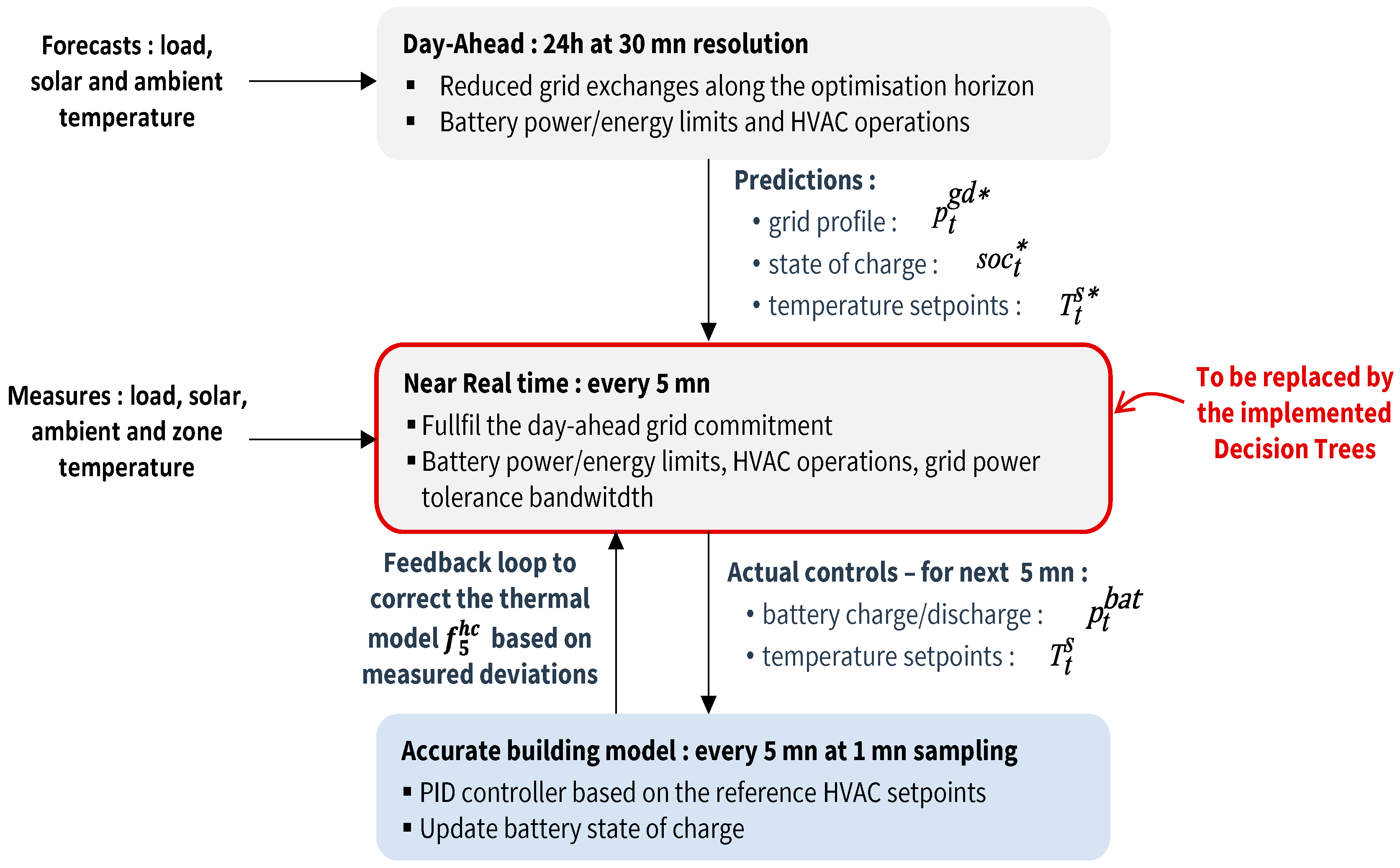
Figure 2 summarizes the work flow of the two-stage MPC previously implemented. Especially, in addition to the mitigation of forecast uncertainties with the real time stage, an online tuning of the 5 min scale thermal model f 5 h c reduces the impact of equations inaccuracies. That tuning relies on a feedback loop that measures the deviations between the predicted HVAC power and the measured value—more details can be found in [22]. As depicted in (3), that feedback estimates the error between (i) the HVAC power value predicted (~) by the MPC equations in the near-real time stage and (ii) the actual value measured once the near real-time controls are applied to the reference building model (i.e., accurate equations). This error et in integrated along time and used to adapt the model equations for the HVAC cooling (4) and heating (5) powers considered in the MPC problem (2).
e t = e t 1 + p t h t p ˜ t h t
p t c a c 5 T a × T t a + a c 5 T s × T t s + a c 5 T z × T t z + b c 5 + e t + 1 u t c × λ p t c a c 5 T a × T t a + a c 5 T s × T t s + a c 5 T z × T t z + b c 5 + e t 1 u t c × λ t T
p t h a h 5 T a × T t a + a h 5 T s × T t s + a h 5 T z × T t z + b h 5 + e t + u t c × λ p t h a h 5 T a × T t a + a h 5 T s × T t s + a h 5 T z × T t z + b h 5 + e t u t c × λ t T
The implementation has proven to be effective to minimize the grid exchanges and maintaining minimal deviations from the commitment in real time. However, as already mentioned in the introduction, a more simple, compact, and lightweight controller is needed to reduce the cost of the hardware and the computational burden in real time. Proposing such a simple controller is the scope of this paper and data driven approaches are envisioned, as they require few computational capabilities once the training is done. As discussed, RL techniques require many interactions with the controlled environments and have shown to lack transparency and deterministic conclusions, hence they are generally unexplainable. In this paper, for explainability and acceptance purposes, simple regression controllers based on Decision Trees are considered and their performances are assessed in terms of precisions against the original MPC performances.

4. Decision Trees’ Implementations, Training, and Tuning

4.1. Investigated Decision Trees (DTs)

4.1.1. Regular DTs

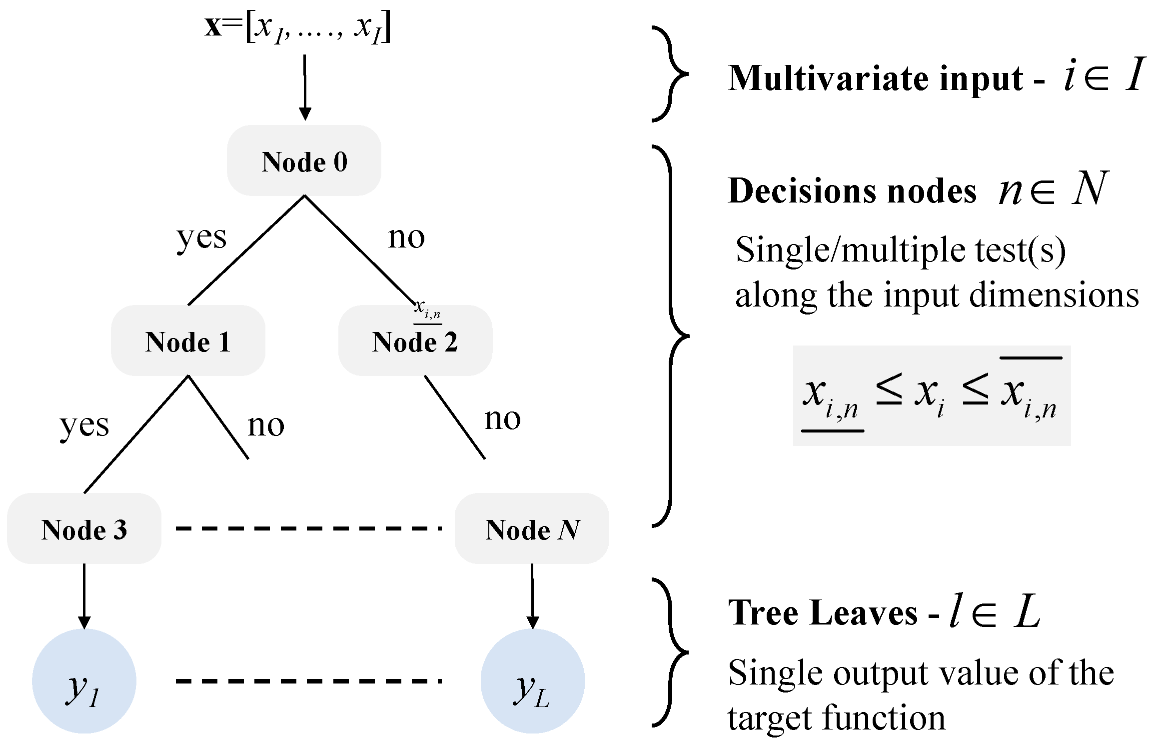
A Decision Tree (DT) is a type of supervised machine learning technique typically used for classification and regression tasks. It works by recursively partitioning the data into subsets based on features that best separate the target y = f(x) [25]. The goal is to create a model that predicts the target variable by learning simple decision rules inferred from the data features x. In the context of power and energy systems, DTs are conventionally used to predict load profile [26] or renewable generation [27]. However, implementations for control applications of microgrid and/or storage systems are gaining interest [28,29]. In such cases, setpoints for controllable assets are computed in real time based on measured values of load and/or generation. Figure 3 illustrates the decision-making process in the case of regular DTs from a multivariate input x (xi in dimension i I ) with successive tests along N decision nodes. The explainability of the DT lies in the simple test performed from the input values with lower/upper threshold values ( x i , n ¯ , x i , n ¯ ) along the input features. Ultimately, the output of the regular DT derives from a termination leave, with a single yl value active at a time following the decisions nodes. As such, in its simplest implementation, the DT procedure can then be seen as a piecewise constant approximation. From a training data set; the fitting process, then, consists of finding the best leaves values and node test conditions in order to better approximate the target function.

4.1.2. Regressor DTs

An extreme gradient-boosting regressor is an ensemble method that combines the result of multiple Decision Trees [30]— d D . Each tree of the ensemble is iteratively trained, and each iteration uses the error residuals of the precious tree to feed the next one. The final output is a weighted sum of the results of all the trees noted yd in the ensemble (weights wd in (6)). The benefit from this is that each tree is shallow and may display small numbers of leaves that an overall single DT performs for the same task, which can allow reduced computational time. The impact of the training process and number of leaves will be discussed in the Results Section.
y = d D w d × y d

4.1.3. Linear Functional DTs

The last type of DTs that will be investigated in this paper for near real-time control relies on functional trees [31]. Those DTs proceed in a very similar way as do regular Decision Trees. However, each leaf or decision node, or both the leaves and the nodes, can embed a function of the inputs. Here, functional DTs will be considered with each leaf displaying a linear function with the input values as in (7). The linear coefficient ai,l and bl for each of the leaves are computed in the course of the training.
y l = i I a i , l × x i + b l

4.2. Investigated Implementations

4.2.1. Inputs/Outputs

The previous subsection discussed the DTs variations that will be investigated. As mentioned and illustrated on Figure 2, the objective is to replace the near real-time MPC with a solution based on DTs. Thus, the target function from the tree perspective is to estimate the setpoints values to send to the battery and HVAC system, as in (8).
y = p t b a t , T t s
As for the inputs to consider for the real-time controller, it is important to note that theoretically, there could be infinite possibilities to test with different combinations of current and past measurements values, predictions, and control settings. Preliminary studies have been carried out with a wide range of settings; thus, this paper investigates only three inputs for the sake of clarity. Then, (9) displays a first input vector x0 that is considered with predicted values from the first stage MPC (upperscript “*”), instantaneous measurements (load, generation and temperature) and previous values for the soc, one, and setpoint temperatures. A second set of input is tested x1 in (10) that identifies the time index with a sinus wave at any time step the real time controller is run. The third input test x2 in (11) considers the time through a sinus along with more information on the reference values for the temperature setpoints and state of charge (coming from the first stage MPC). The overall objective here is then to properly choose the best input to consider in terms of relevant information for the real time control. This will be discussed while assessing the performances of different implementations of the decision tree controllers—i.e., different inputs, DT parameters, and training sets.
x 0 = p t g d * s o c t * T t s * p t l p t p v T t a s o c t 1 T t 1 z T t 1 s
x 1 = sin w t p t g d * p t l p t p v T t a s o c t 1 T t 1 z
x 2 = sin w t p t g d * s o c t * T t s * p t l p t p v T t a s o c t 1 T t 1 z T t 1 s

4.2.2. Training Based on MPC Historical Results

From the previous discussions, DTs can, then, be roughly seen as a mapping between inputs and outputs. Training datasets for both input/outputs are then needed in the training process. A first implementation makes uses of the stage MPC to generate the datasets. The MPC is simulated along one year—i.e., along 365 successive days with both look-ahead and near real-time stages—and the obtained data are partitioned as follows:
  • ▪ Training Set A: 1 month (Jan)
  • ▪ Training Set B: 5 months (Jan–May)
  • ▪ Testing Set: 7 months (Jun–Dec)
Two training sets A and B will be investigated in order to assess the impact of the amount of input information.

4.2.3. Training Based on Model and Online Tuning

The implementation method previously mentioned implies that we will run the original MPC on the actual system in order to generate the training data set. However, this is not deemed an ideal scenario. If the actual deployment of the original MPC is required to train the DT, the need for a faster lightweight real-time controller is arguable. Thus, a more realistic setup includes training the DTs in an offline mode with the two stage MPC run with historical forecast and measurements (load, solar, and ambient temperature) but with the coarse thermal model only ( f 30 h c and f 5 h c ). Specifically, the near real-time stage MPC does not benefit from the online adaptation of the model equations, thanks to feedback measurements as in Figure 2.
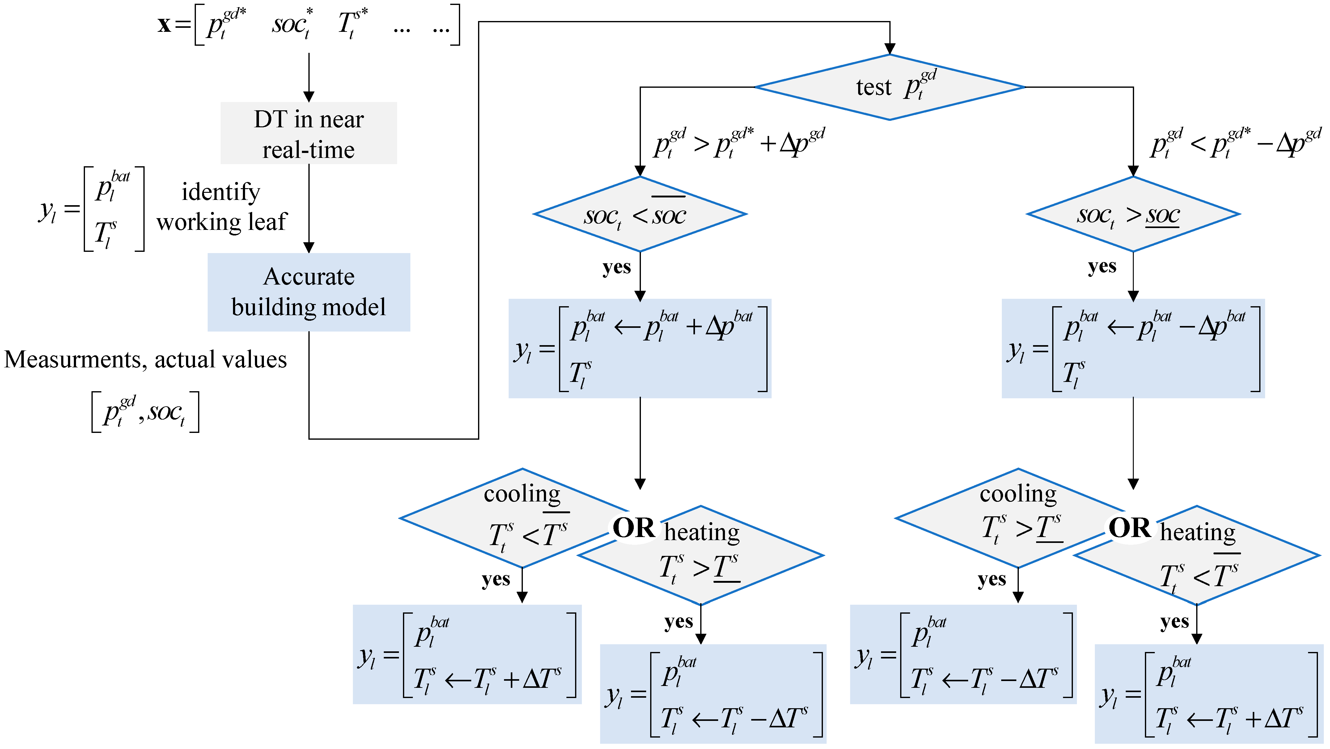
In addition to that offline tuning, to improve the expected performances of the controller, an online strategy is proposed to tune the pre-trained DT once it is deployed on the building. Figure 4 details the flowchart of the proposed tuning. It adjusts the leaf output values yl = [ p l bat , T l s ] based on the observations after the controls are sent to the actual system—i.e., the reference thermal model f r e f h c . Once the controls are applied to the system, the actual grid power value p t g d * is measured. If it is beyond the tolerance bandwidth Δ p g d there are then successive tests to identify if controls could have been improved and the output of the operating DT leaf are updated accordingly. The tests account for the upper/lower bounds for the state of charge ( s o c _ , s o c ¯ ) and zone temperature setpoints ( T s _ , T s ¯ ). For instance, if the grid power is above the tolerance after the leaf control are applied, and the battery is not fully discharged, its power can then be increased with an increment parameter Δ p b a t . To further bring the grid power closer to the commitment when needed, if the HVAC operated in cooling mode (resp. heating mode), the temperature setpoints for the operating leaf can be increased (resp. decreased) with an increment parameter Δ T s . Similarly, the leaf output values are updated to increase the grid power profile if it is below the tolerance bandwidth. As such, the proposed tuning of the leaf output values can be seen as an integral corrector based on the deviations along time. It is also important to note that only one leaf at a time (i.e., the operating leaf) is updated if any further improvement can be made within the operating limits of the equipment. The impact of the increment parameters of the tuning (i.e., Δ p p a t and Δ T s ) will be discussed in the Discussions Section of the paper.

5. Results and Discussions

5.1. Input Data and Performance Metrics

In addition to the system and algorithm parameters (e.g., storage/HVAC characteristics, room layout, algorithm settings), the case study simulation relies on open data sets. The household electrical load profiles are taken from the REFIT data set (https://pureportal.strath.ac.uk/en/datasets/refit-electrical-load-measurements-cleaned—URL accessed on 21 April 2024) [32] and weather data from NOAA website (https://www.ncei.noaa.gov/access/crn/—URL accessed on 21 April 2024) [33] We are reminded that the weather data consist in solar radiation and outdoor temperature profiles to further compute the photovoltaic generation and HVAC consumption.
The two metrics considered to assess the performances of the proposed controllers (original MPC and DT implementations) follow the objectives targeted by the overall control scheme. At first, E2 in kWh2 denotes the energy exchanges with the upstream grid following the objective of the first MPC stage (12). It is important to note that the real-time stage impacts that objective once the system is actually controlled, and due to forecast errors and mitigation actions, the ultimate E2 values differ from the first stage prediction. The second performance metric quantifies the errors with the commitment on the grid power profile with Edev (in kWh) that accounts for the deviations beyond the tolerance bandwidth (13). Note that both metrics can be computed along different temporal horizons, days, months, and years, depending on the granularity of the result analysis.
E 2 = t T p t g d 2 × d t
E d e v = t T δ + + δ × d t   with   δ + = p t g d p t g d * + Δ p g d   if   p t g d > p t g d * + Δ p g d δ = p t g d * Δ p g d p t g d   if   p t g d < p t g d * Δ p g d

5.2. Training on Historical MPC

This subsection presents the results obtained with the different DT implementations and while training based on the original MPC deployed on the actual building. The impact of the training period, input type, and DT architectures will be discussed.

5.2.1. Regular DTs

Figure 5 and Figure 6 display the results obtained with the second stage of the control run using regular DTs. Overall, the performances improve significantly with the number of leaves with decreasing performances metrics. However, it is important to note that both E2 and Edev values remain higher than the ones obtained with the original real-time MPC (considered as a reference here). From 200 leaves onwards, there is no significant improvement of the two metrics. Also, the impact of both the training set duration and input types is marginal compared to the number of leaves. The results obtained with the sets of inputs x0 and x2 are very close (if not identical), which suggests that the consideration of the time index as input is not very important for the application considered. Training along five months slightly improves the performance obtained over the seven-months test period.

5.2.2. Regressor DTs

Figure 7 and Figure 8 display the results obtained from the second stage of the control run using regressor DTs. Results shall be analyzed regarding the total number of leaves—i.e., the number of trees multiplied by the number of leaves in every tree. Similar to the previous regular DT, increasing the number of leaves significantly improves the performance up to a certain point—in this case, 150 leaves, which is in the same range as the one observed in the previous regular case. More importantly, the overall performances of regressor DT appears much better than the results of regular DTs with smaller values for both E2 and Edev. The metric on the energy exchanges is even better than the reference performance obtained with the original two-stage MPC. As before, the difference between results with inputs x0 and x2 is not significant (if not null). The increased training set duration allows marginal improvement of the Edev metric at the cost of greater E2 values. Also, training along five months slightly improves the performance on the energy deviation.

5.2.3. Linear DTs

Figure 9 and Figure 10 display the results obtained when implementing linear DTs. Compared to the results from the regular and regressor DTs, the first noticeable outcome is that the performances depicted are obtained with very small numbers of leaves in comparison to the previous implementations with 10 leaves only or less. Again, results for inputs x0 and x2 are identical, and training along five months slightly improve the performances. The most noticeable outcome is that the best values obtained over all the tests performed in this section for all DTs implementations are obtained with the linear DT controller with four leaves. This configuration will then be further considered for the training on model-only, followed by the online tuning of the controller.

5.3. Training on Model MPC and Online Tuning

5.3.1. Controller Performances

From the previous results, Linear DTs significantly outperform the other implementations for the considered application. However, the previous results were obtained while training the controllers from outputs of the overall two-stage MPC. This then requires the actual operation of the reference MPC along a given period (one- or five-month training periods being investigated). In such a case, the interest in a lightweight real-time controller would then be arguable in replacement of a second stage MPC that would have to be implemented. Thus, and as already been mentioned, this paper investigates a more realistic setup, in which the DT based controller (linear DT) is trained on a model of the actual system only. In practice, as illustrated on Figure 2, this bypasses the feedback loops that allow refining of the models in the original two-stage MPC. However, training on a coarse model obviously degrades the performances of the Linear DT once applied to the actual building, as depicted in Figure 11. Both performance metrics significantly increase when training on models only, instead of training with the historical values obtained from the operation of the original MPC. Results are obtained while considering the input set x2 as it displays the best performance.
In order to improve the performance of the Linear DT-based controller trained on model only, the paper proposes the online tuning strategy of Section 4.2.3. The proposed methodology consists of adjusting the weightages in the output leaves from the observations once the controls are applied to the actual building controlled. In this section, a Linear DT with four leaves using the input set x2 trained along five months on models is considered as a starting point before being improved online. Table 1 displays the average daily performances for the two metrics considered and with different implementations of the near real-time control. As previously observed, the training of a Linear DT, based on model-only, significantly degrades the performance compared to a training on historical MPC (5 months of training), with both the E2 (+21%) and the Edev (+26%) values being greater. With the online tuning proposed, both metrics greatly improve but without meeting the best values obtained with the original MPC. However, the lightweight DT tuned online displays a deviation metric even better than that of the version trained on historical data from the MPC.
All the results previously discussed considered daily average values of the performance metrics over the 7-month test period. However, the results vary along the test period depending on the forecast accuracy in the day-ahead phase and the volatility of daily profiles in real time. Figure 12, then, illustrates the daily values of both E2 and Edev in terms of errors with the original MPC performances. As such, positive values in some cases identify days in which the proposed controller performs even better than the original MPC. Overall, the figure highlights that in most days, tuning the Linear DT online significantly improves the Edev metric compared to a controller trained offline only. However, the results towards the end of the test period show that in most cases, the E2 criteria is significantly degraded with the Linear DT tuned online, which illustrates the increase of the daily average value observed in Table 1.

5.3.2. Discussions

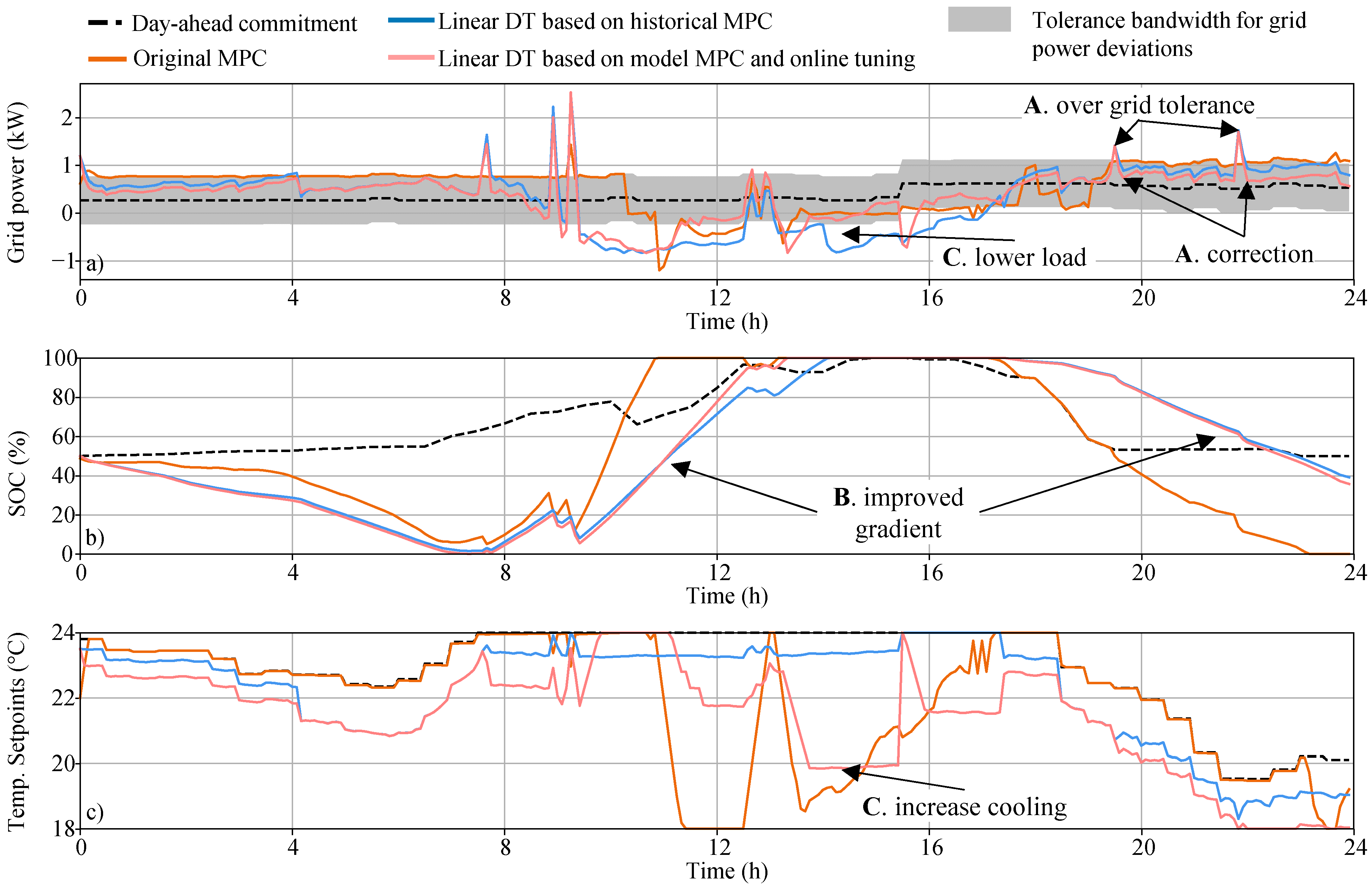
To further illustrate the control results and the impact of the Linear DT online tuning, Figure 13 displays time series profiles along a single autumn day. For the grid power profile, Figure 13a shows that the online tuning strategy allows to decrease the deviation with the commitment—deviations beyond the tolerance bandwidth highlighted in grey. Compared to a DT trained offline only, downward deviations are strongly reduced in the middle of the day (points A). From Figure 13b,c, it appears that most differences between the DT trained offline only, and the implementation tuned online, lie on the modification of the temperature setpoints. Indeed, variations in state of charge are marginal, with charge/discharge rates slightly increased (points B). Differences in temperature setpoints are much more significant. Especially in the middle of the day, the setpoint reduction leads to greater HVAC consumption in order to bring the grid power closer to the day-ahead commitments (points C).
Ultimately, the performance of the online tuning proposed depends on the increment parameters. Before displaying the results discussed previously, a sensitivity analysis was performed in order to find the most appropriate values for the increment parameters in the tuning process (i.e., Δ p p a t and Δ T s ). Figure 14 displays the results obtained for the two performance metrics along the test period with different sets of tuning parameters. This highlights the solutions considered for the results discussed in the previous subsection. However, it is worth noting that deviation from this best setting significantly degrades the performances. In the worst cases (e.g., Δ p p a t = 0.05 kW and Δ T s = 0.05   ° C ), the metrics values could even be worse than the Linear DT trained on model only without tuning. Also, following the obtained results for all the values investigated, no instability of the controller, as noticed in terms of unrealistic controls (storage and HVAC), was detected. The continuous update of the controller relies on increments that are significantly lower than the rated storage power and bounds for temperature setpoints. Also, the controls, ultimately sent to the systems, are limited, with dedicated saturation blocks. Further immediate studies shall, then, focus on the conservativeness of the tuning parameters for other use cases and/or longer periods of time, which is beyond the scope of this paper.
Based on the results obtained, it is possible to qualitatively discuss the pros and cons of the different DT implementation and MPC investigated in the paper (Table 2). As already mentioned, a single run of the MPC last around 1–2 s where the DT commutations is almost instantaneous. The DT training never exceeds 5 s, as it consists in simple models. Indeed, that simplicity and explainability drove our research to investigate DT first, before considering other AI techniques such as supervised learning with neural networks. Indeed, DTs distinguish themselves with very few training parameters and the outputs can be easily interpreted form the inputs—as an example, linear DTs proved to reach good performances with four leaves only, i.e., four linear combinations with the input features. Overall, in terms of “coding”, the DTs variations are very easy to implement. However, the versions that require a training with actual output from the original MPC are, then, not helpful in practice. That motivated the approach that was trained on a model of the system, without the need to send controls to the actual building.

6. Conclusions

This paper investigates the implementations of data-driven controllers for the near real-time control of a HVAC and storage system in a residential building. The article builds upon previous work from the authors that implemented a two stage MPC with (i) a day-ahead optimal scheduling based on model and optimization and (ii) a real-time AI-based control to fulfill the commitment from the first stage. The objective is to investigate lightweight controllers for the real-time stage to replace the MPC that relies on model and optimization (i.e., non-negligible computational effort). To do so, Decisions Trees (DTs) are considered, as they provide explainable solutions with outputs computed from a sequence of explicit tests on input data with thresholds. Several variations are investigated with regular, regressor and linear DTs. The last proved to lead to the best performances with a very low degree of complexity—i.e., with a small number of leaves. When trained on historical MPC, linear DTs show even greater performances in term of energy exchanges than the reference MPC do. However, with such implementation being unrealistic, an offline training of the DT is proposed. This avoids the need for the actual deployment of the original MPC at the cost of reduced performance. An online tuning strategy is then implemented and relies on an online update of the leaves coefficients, based on observations. This allows the linear DT to significantly improve the performances, regarding the energy deviation in real time with the look-ahead commitment (−25% less deviations). The work was carried out in the framework of a project dealing with the coordinated control of multiple buildings. Further works will, then, propose DT-based control in the scope of multi-player environments. Also, a research area seems promising, while investigating the impact of the original model accuracy in the context of offline training. In other words, a question remains open on which model precisions are needed for offline training in order to guarantee acceptable performances. In some cases, no accurate models may be available, and it is deemed important to assess the impact on the training performances.

Author Contributions

R.R.-M.—conceptualization, methodology, resources, writing, visualization, supervision, funding acquisition; A.Y.—methodology, software, validation, writing. All authors have read and agreed to the published version of the manuscript.

Funding

This work has been carried out in the framework of the INT2MEC project—INTelligent Multi-Energy Communities for enhanced distributed resources INTegration in Singapore (Seed Project ITS009-0019). The research is supported by the National Research Foundation, Prime Minister’s Office, Singapore under its Campus for Research Excellence and Technological Enterprise (CREATE) program.

Data Availability Statement

Data will be made available upon request.

Conflicts of Interest

Alim Yakub was employed by CNRS@CREATE in Singapore, Rémy Rigo-Mariani is affiliated to CNRS@CREATE and employed by CNRS in France. The remaining authors declare that the research was conducted in the absence of any commercial or financial relationships that could be construed as a potential conflict of interest. The authors declare no conflicts of interest. The funders had no role in the design of the study; in the collection, analyses, or interpretation of data; in the writing of the manuscript; or in the decision to publish the results.

References

  1. ‘Renewables 2023—Analysis’, IEA. Available online: https://www.iea.org/reports/renewables-2023 (accessed on 5 March 2024).
  2. Vasiliev, M.; Nur-E-Alam, M.; Alameh, K. Recent Developments in Solar Energy-Harvesting Technologies for Building Integration and Distributed Energy Generation. Energies 2019, 12, 1080. [Google Scholar] [CrossRef]
  3. Klingler, A.-L. Self-consumption with PV + Battery systems: A market diffusion model considering individual consumer behaviour and preferences. Appl. Energy 2017, 205, 1560–1570. [Google Scholar] [CrossRef]
  4. Huy, T.H.B.; Dinh, H.T.; Kim, D. Multi-objective framework for a home energy management system with the integration of solar energy and an electric vehicle using an augmented ε-constraint method and lexicographic optimization. Sustain. Cities Soc. 2023, 88, 104289. [Google Scholar] [CrossRef]
  5. Mir, U.; Abbasi, U.; Mir, T.; Kanwal, S.; Alamri, S. Energy Management in Smart Buildings and Homes: Current Approaches, a Hypothetical Solution, and Open Issues and Challenges. IEEE Access 2021, 9, 94132–94148. [Google Scholar] [CrossRef]
  6. Dadashi-Rad, M.H.; Ghasemi-Marzbali, A.; Ahangar, R.A. Modeling and planning of smart buildings energy in power system considering demand response. Energy 2020, 213, 118770. [Google Scholar] [CrossRef]
  7. Ghayour, S.S.; Barforoushi, T. Optimal scheduling of electrical and thermal resources and appliances in a smart home under uncertainty. Energy 2022, 261, 125292. [Google Scholar] [CrossRef]
  8. Gholamzadehmir, M.; Del Pero, C.; Buffa, S.; Fedrizzi, R.; Aste, N. Adaptive-predictive control strategy for HVAC systems in smart buildings—A review. Sustain. Cities Soc. 2020, 63, 102480. [Google Scholar] [CrossRef]
  9. Di Piazza, M.; La Tona, G.; Luna, M.; Di Piazza, A. A two-stage Energy Management System for smart buildings reducing the impact of demand uncertainty. Energy Build. 2017, 139, 1–9. [Google Scholar] [CrossRef]
  10. Blad, C.; Bøgh, S.; Kallesøe, C.S. Data-driven Offline Reinforcement Learning for HVAC-systems. Energy 2022, 261, 125290. [Google Scholar] [CrossRef]
  11. Pinto, G.; Deltetto, D.; Capozzoli, A. Data-driven district energy management with surrogate models and deep reinforcement learning. Appl. Energy 2021, 304, 117642. [Google Scholar] [CrossRef]
  12. Lork, C.; Li, W.-T.; Qin, Y.; Zhou, Y.; Yuen, C.; Tushar, W.; Saha, T.K. An uncertainty-aware deep reinforcement learning framework for residential air conditioning energy management. Appl. Energy 2020, 276, 115426. [Google Scholar] [CrossRef]
  13. Yang, L.; Li, X.; Sun, M.; Sun, C. Hybrid Policy-Based Reinforcement Learning of Adaptive Energy Management for the Energy Transmission-Constrained Island Group. IEEE Trans. Ind. Inform. 2023, 19, 10751–10762. [Google Scholar] [CrossRef]
  14. Arroyo, J.; Manna, C.; Spiessens, F.; Helsen, L. Reinforced model predictive control (RL-MPC) for building energy management. Appl. Energy 2022, 309, 118346. [Google Scholar] [CrossRef]
  15. Kumar, S.R.; Easwaran, A.; Delinchant, B.; Rigo-Mariani, R. Behavioural cloning based RL agents for district energy management. In Proceedings of the 9th ACM International Conference on Systems for Energy-Efficient Buildings, Cities, and Transportation, in BuildSys ’22, Boston, MA, USA, 9–10 November 2022; Association for Computing Machinery: New York, NY, USA, 2022; pp. 466–470. [Google Scholar] [CrossRef]
  16. Chen, B.; Cai, Z.; Berges, M. Gnu-RL: A Practical and Scalable Reinforcement Learning Solution for Building HVAC Control Using a Differentiable MPC Policy. Front. Built Environ. 2020, 6, 562239. [Google Scholar] [CrossRef]
  17. Ngarambe, J.; Yun, G.Y.; Santamouris, M. The use of artificial intelligence (AI) methods in the prediction of thermal comfort in buildings: Energy implications of AI-based thermal comfort controls. Energy Build. 2020, 211, 109807. [Google Scholar] [CrossRef]
  18. Zhang, Z.; Chong, A.; Pan, Y.; Zhang, C.; Lam, K.P. Whole building energy model for HVAC optimal control: A practical framework based on deep reinforcement learning. Energy Build. 2019, 199, 472–490. [Google Scholar] [CrossRef]
  19. Panda, S.P.; Genest, B.; Easwaran, A.; Rigo-Mariani, R.; Lin, P. Methods for mitigating uncertainty in real-time operations of a connected microgrid. Sustain. Energy Grids Netw. 2024, 38, 101334. [Google Scholar] [CrossRef]
  20. El Maghraoui, A.; Ledmaoui, Y.; Laayati, O.; El Hadraoui, H.; Chebak, A. Smart Energy Management: A Comparative Study of Energy Consumption Forecasting Algorithms for an Experimental Open-Pit Mine. Energies 2022, 15, 4569. [Google Scholar] [CrossRef]
  21. Kontogiannis, D.; Bargiotas, D.; Daskalopulu, A. Fuzzy Control System for Smart Energy Management in Residential Buildings Based on Environmental Data. Energies 2021, 14, 752. [Google Scholar] [CrossRef]
  22. Rigo-Mariani, R.; Ahmed, A. Smart home energy management with mitigation of power profile uncertainties and model errors. Energy Build. 2023, 294, 113223. [Google Scholar] [CrossRef]
  23. Troitzsch, S. kaiATtum, tomschelo, and arifa7med, mesmo-dev/mesmo: Zenodo. 2021. Available online: https://zenodo.org/record/5674243 (accessed on 11 April 2023).
  24. Kirschen, D.; Strbac, G. Fundamentals of Power System Economics—Daniel S. Kirschen, Goran Strbac—Google Books, 2nd ed. Wiley. 2018. Available online: https://books.google.fr/books/about/Fundamentals_of_Power_System_Economics.html?id=rm61AAAAIAAJ&source=kp_book_description&redir_esc=y (accessed on 2 March 2022).
  25. Quinlan, J.R. Induction of decision trees. Mach. Learn. 1986, 1, 81–106. [Google Scholar] [CrossRef]
  26. Jahan, I.S.; Snasel, V.; Misak, S. Intelligent Systems for Power Load Forecasting: A Study Review. Energies 2020, 13, 6105. [Google Scholar] [CrossRef]
  27. Meenal, R.; Binu, D.; Ramya, K.C.; Michael, P.A.; Kumar, K.V.; Rajasekaran, E.; Sangeetha, B. Weather Forecasting for Renewable Energy System: A Review. Arch. Comput. Methods Eng. 2022, 29, 2875–2891. [Google Scholar] [CrossRef]
  28. Moutis, P.; Skarvelis-Kazakos, S.; Brucoli, M. Decision tree aided planning and energy balancing of planned community microgrids. Appl. Energy 2016, 161, 197–205. [Google Scholar] [CrossRef]
  29. Luo, X.; Xia, J.; Liu, Y. Extraction of dynamic operation strategy for standalone solar-based multi-energy systems: A method based on decision tree algorithm. Sustain. Cities Soc. 2021, 70, 102917. [Google Scholar] [CrossRef]
  30. XGBoost|Proceedings of the 22nd ACM SIGKDD International Conference on Knowledge Discovery and Data Mining. Available online: https://dl.acm.org/doi/10.1145/2939672.2939785 (accessed on 25 March 2024).
  31. Gama, J. Functional Trees. Mach. Learn. 2004, 55, 219–250. [Google Scholar] [CrossRef]
  32. Murray, D.; Stankovic, L.; Stankovic, V. An electrical load measurements dataset of United Kingdom households from a two-year longitudinal study. Sci. Data 2017, 4, 160122. [Google Scholar] [CrossRef]
  33. Diamond, H.J.; Karl, T.R.; Palecki, M.A.; Baker, C.B.; Bell, J.E.; Leeper, R.D.; Easterling, D.R.; Lawrimore, J.H.; Meyers, T.P.; Helfert, M.R.; et al. U.S. Climate Reference Network after One Decade of Operations: Status and Assessment. Bull. Am. Meteorol. Soc. 2013, 94, 485–498. Available online: https://journals-ametsoc-org.sid2nomade-1.grenet.fr/view/journals/bams/94/4/bams-d-12-00170.1.xml (accessed on 11 April 2023). [CrossRef]
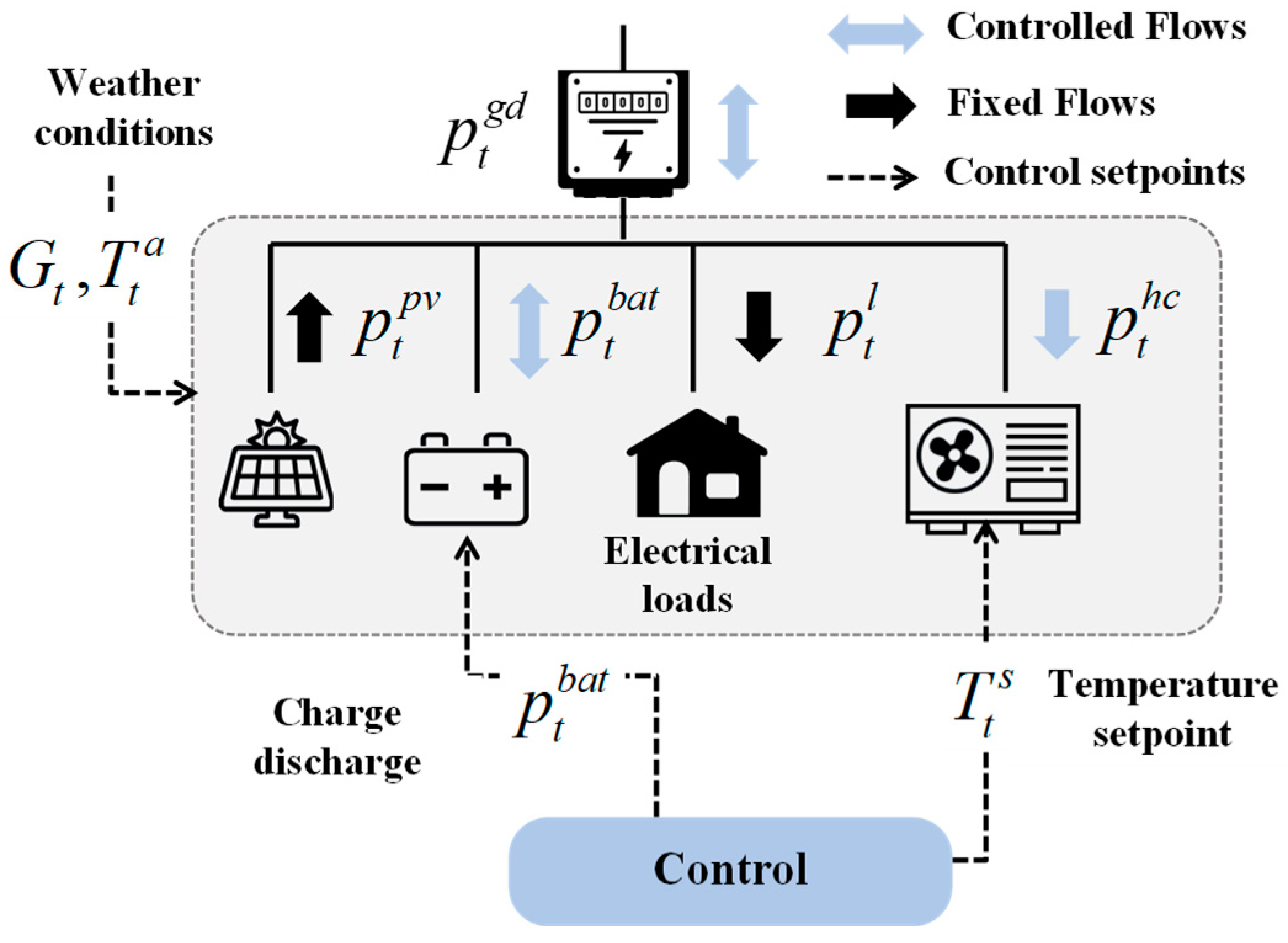
Figure 1. Controlled Residential Building (derived from [22]).
Energies 17 02730 g001
Figure 2. Flowchart of the baseline two-stage MPC (derived from [22]).
Energies 17 02730 g002
Figure 3. Regular DT architecture.
Energies 17 02730 g003
Figure 4. Flowchart of the tuning strategy.
Energies 17 02730 g004
Figure 5. Regular DTs with different input types and number of leaves with 1-month training—(a) E2—(b) Edev.
Energies 17 02730 g005
Figure 6. Regular DTs with different input types and number of leaves with 5-months of training—(a) E2—(b) Edev.
Energies 17 02730 g006
Figure 7. Regressor DTs with different input types and number of leaves with 1-month of training—(a) E2—(b) Edev.
Energies 17 02730 g007
Figure 8. Regressor DTs with different input types and number of leaves with 5-month training—(a) E2—(b) Edev.
Energies 17 02730 g008
Figure 9. Linear DTs with different input types and number of leaves with 1-month of training—(a) E2—(b) Edev.
Energies 17 02730 g009
Figure 10. Linear DTs with different input types and number of leaves with 5-month training—(a) E2—(b) Edev.
Energies 17 02730 g010
Figure 11. Linear DT performances while training with (historical) and without (model) feedback loop in the MPC—(a) E2—(b) Edev.
Energies 17 02730 g011
Figure 12. Daily performances error with reference MPC—(a) E2—(b) Edev.
Energies 17 02730 g012
Figure 13. Control results along one autumn day for different real-time implementations—(a) grid power—(b) state off charge—(c) temperature setpoint.
Energies 17 02730 g013
Figure 14. Performances of the Linear DT trained on model and tuned online with different tuning parameters—(a) E2—(b) Edev.
Energies 17 02730 g014
Table 1. Average daily performances for different near real-time controllers.
E2 (kWh2)Edev (kWh)
Reference MPC and online tuning30.501.63
Linear DT based on historical MPC data30.182.34
Linear DT based on model MPC data36.652.94
Linear DT based on model MPC and online tuning33.822.19
Table 2. Comparative study of near real-time control implementations.
Historical TrainingModel TrainingMPC
Regular
DTs
Regular
DTs
Linear
DTs
Linear
DTs
Linear DTs + Tuning
Performances Metric E2+++ +++ +
Performances Metric Edev+++ +++ +
Implementation+ +++
Running Time+ ++++ ++ ++ +
Explainability+ ++ ++ ++ +
Training Time+ ++++ ++ ++ +N.A.
Disclaimer/Publisher’s Note: The statements, opinions and data contained in all publications are solely those of the individual author(s) and contributor(s) and not of MDPI and/or the editor(s). MDPI and/or the editor(s) disclaim responsibility for any injury to people or property resulting from any ideas, methods, instructions or products referred to in the content.