Predicting the Remaining Useful Life of Solid Oxide Fuel Cell Systems Using Adaptive Trend Models of Health Indicators

Abstract

Degradation is an inevitable companion in the operation of solid oxide fuel cell (SOFC) systems since it directly deteriorates the reliability of the system’s operation and the system’s durability. Both are seen as barriers that limit the extensive commercial use of SOFC systems. Therefore, diagnosis and prognosis are valuable tools that can contribute to raising the reliability of the system operation, efficient health management, increased durability and implementation of predictive maintenance techniques. Remaining useful life (RUL) prediction has been extensively studied in many areas like batteries and proton-exchange membrane fuel cell (PEM) systems, and a range of different approaches has been proposed. On the other hand, results available in the domain of SOFC systems are still relatively limited. Moreover, methods relying on detailed process models and models of degradation turned out to have limited applicability for in-field applications. Therefore, in this paper, we propose an effective, data-driven approach to predicting RUL where the trend of the health index is modeled by an adaptive linear model, which is updated at all times during the system operation. This allows for a closed-form solution of the probability distribution of the RUL, which is the main novelty of this paper. Such a solution requires no computational load and is as such very convenient for the application in ordinary low-cost control systems. The performance of the approach is demonstrated first on the simulated case studies and then on the data obtained from a long-term experiment on a laboratory SOFC system. From the tests conducted so far, it turns out that the quality of the RUL prediction is usually rather low at the beginning of the system operation, but then gradually improves while the system is approaching the end-of-life (EOL), making it a viable tool for prognosis.

1. Introduction

SOFC systems represent an attractive technology for the conversion of electrochemical energy into electrical power due to lower emissions, high efficiency, useful waste heat and fuel flexibility. They are being widely applied in auxiliary power unit (APU) and stationary power generators [1]. Yet, the most significant barriers to their broader commercialization and market deployment are insufficient durability, reliability and cost. Reliability and durability, in particular, are significantly impacted by the degradation phenomena that emerge during the operation at high temperatures.

Understanding the mechanisms that cause the deterioration is of paramount importance for the design, operation and management of the SOFC systems. Much of the research endeavors have been focused on modeling the multiphysics and multiscale processes from micro-structural to system level to understand the conditions that cause the degradation and its rate as well as the relationship with the reliability and the life span [2,3]. Due to the complexity of the underlying models and the required computational load, their use in online diagnosis and prognosis is not feasible.

Thanks to the increasing volume of historical data acquired from the rising number of SOFC systems under test in the laboratory and in situ operation, room for the use of different machine learning approaches to either predict the degradation trend or estimate the RUL has become widely open. In particular, strong research and development of methods of prognosis have been conducted in the related areas of battery research and, to a lesser extent, in the domain of fuel cells. A comprehensive survey of prognostic methods for batteries can be found in [4]. For example, in [5] over 20,000 electrochemical impedance spectroscopy (EIS) spectra of commercial Li-ion batteries, collected at different states of health, states of charge and temperatures were applied to a machine learning algorithm to automatically determine which spectral features predict degradation and the remaining life.

Although less intensive compared to the batteries, the amount of research in data-driven prognostics in PEM is still rather solid and a variety of machine learning techniques have been proposed. A good overview can be found in [6].

To date, considerably less attention has been paid to the development of algorithms for online prediction of RUL in SOFC systems, so the list of references is rather constrained. A brief address can be found in the review paper [7].

In an early attempt, in [8], the authors adopt a neural network model in which time is used as an explicit independent variable to describe the decay of voltage as a function of time and operational parameters. The authors in [9] study the RUL prediction under two degradation modes, i.e., anode poisoning and cathode humidification. From a series of simulated life-long tests, they learn the parameters of the transition model by the data-driven method (least squares support vector machine). However, a change in the health metric, voltage in this case, can be directly affected by operating conditions imposed on the system. Therefore, it is difficult to distinguish whether it is caused by the degradation of the fuel cells, a change in load condition or if it is a response of the system due to a controller action.

Deriving the data-driven model of the stack voltage as a function of the process variables has been pursued in [10] by using a dynamic neural network model. The idea is to train the model in the nominal condition and then take the discrepancy between measured and reconstructed stack voltage as a health indicator and anticipate its trend. In an alternative study by Zhang et al. [11], the authors present a data-driven approach for fault prognostics in SOFC systems. They employ voltage signal analysis and statistical modeling to forecast end-of-life scenarios and substantiate their predictions through post-mortem microscopy analysis.

In [12], the health indicator is associated with the area specific resistance (ASR), which is largely affected by the stack degradation and can be made mostly invariant to the process variables. The idea is based on a simple premise that the degradation can be viewed as a hidden random walk process. To deconvolute the degradation dynamics from the available process data, the authors developed a nonlinear lumped model of the process and the black-box model of the degradation dynamics. By using filtering techniques, the temporal evolution of the ASR is obtained. Based on that, the RUL predictions are evaluated using Monte Carlo (MC) simulation. Similar efforts are evident in Cui et al. [13], employing a particle filter for ASR estimation. This method demonstrates superior accuracy in contrast to the Kalman filtering approach. In an attempt to include more prior knowledge in the degradation model, in [14], the authors showed that under proper conditions the quality of prognostics can be slightly improved compared to the pure black box model. Similarly, in Xu et al. [15], the authors propose a model-based fault prognosis method for SOFC that combines degradation modeling and particle filtering to estimate the state of health (SOH), EOL, and RUL.

The hidden random walk models of the degradation might face two issues. First, it should be noted that a range of phenomenological models has been proposed in [16] based on a thorough investigation of the degradation phenomena under accelerated tests. The decision of which model to apply depends on the correct identification of the degradation mode. Incorrect diagnosis implicates the use of the incorrect degradation model, which might, in turn, lead to misleading results. Second, it can happen in practice that one degradation mode eventually unfolds other degradation modes so that such cascades are immensely difficult to identify.

Moreover, from past experimental runs, it seems the degradation progresses mainly as a monotone process [17] or even a piece-wise linear one [18]. Once the health indicator is selected, the prediction of its future evaluation can be anticipated by using time series analysis tools. In the quest to find the optimum trade-off between the simplicity of the prognostic algorithm and the quality of the prognosis, in this paper, we apply a probabilistic linear trend analysis. The idea is to estimate the local trend using ordinary least squares (OLS) and then estimate the RUL as the time when the health indicator is anticipated to hit a limit value that marks the beginning of the failure state. A novelty of this approach is that the distribution of the first-hitting time (FHT) can be expressed in closed form meaning that the computational load is almost nil. Thus, the algorithm can be easily applied to industrial controllers with limited computational power.

The paper is structured as follows. In Section 2, the method of estimating a linear trend from the data is presented. Then, the main idea that leads to the closed-form solution of the probability distribution of the FHT from the linear trend model is presented. In Section 3, the performance of the method is demonstrated on the different simulated time series scenarios. Finally, in Section 4, the method is demonstrated on experimental data obtained from a long-term run of a SOFC system.

2. Methodology

2.1. Local Linear Trend Model

The observed degradation metric is taken as a time series. A rectangular window function of length M is used to select a part of the data, usually the latest M measurements. For each instance of windowed data, we propose the latent state of the health index, denoted as x, to behave as a linear function

$$\begin{array}{c}\hfill x\left(t\right)=n+kt,n,k\in \mathbb{R},\end{array}$$

(1)

while the observed state, denoted as y, is just the latent state with superimposed normally distributed white noise

$$\begin{array}{c}\hfill y\left(t\right)=x\left(t\right)+\eta \left(t\right),\eta \left(t\right)\sim \mathcal{N}(0,{\sigma }_{\eta }^2),{\sigma }_{\eta }\in {\mathbb{R}}^{+}.\end{array}$$

(2)

Since we only obtain our measurements at discrete times $t_j,j\in (1,\dots ,N)$, we can rewrite the upper equation matrix to form

$$\begin{array}{c}\hfill Y=\left[\begin{array}{c}y\left(t_{N-M+1}\right)\\ y\left(t_{N-M}\right)\\ ⋮\\ y\left(t_N\right)\end{array}\right]=F\left[\begin{array}{c}n\\ k\end{array}\right]+\left[\begin{array}{c}\eta \left(t_{N-M+1}\right)\\ \eta \left(t_{N-M}\right)\\ ⋮\\ \eta \left(t_N\right)\end{array}\right],\mathrm{where}F=\left[\begin{array}{c}1,t_{N-M+1}\\ 1,t_{N-M}\\ ⋮\\ 1,t_N\end{array}\right].\end{array}$$

(3)

From the well-known OLS theory [19], it follows that the most likely value of ${[n,k]}^{\top }$, denoted as Z, is

$$\begin{array}{c}\hfill \mathrm{E}\left[\begin{array}{c}n\\ k\end{array}\right]=Z={\left(F^{\top }F\right)}^{-1}{F}^{\top }Y,\end{array}$$

(4)

the uncertainty of ${[n,k]}^{\top }$, denoted as R, is

$$\begin{array}{c}\hfill \mathrm{Cov}\left[\begin{array}{c}n\\ k\end{array}\right]=R={\left(F^{\top }F\right)}^{-1}{\sigma }_{\eta }^2,\end{array}$$

(5)

and the noise level is

$$\begin{array}{c}\hfill {\sigma }_{\eta }^2=\frac{1}{M-2}{(Y-FZ)}^{\top }(Y-FZ).\end{array}$$

(6)

2.2. Distribution of the Ratio of Two Jointly Normal Variables

Again, the degradation with time, denoted as $x\left(t\right)$, is modeled as a linear function with slope k and intercept n. To account for the uncertainty of the said two parameters, we consider them probabilistic. Their joint distribution is taken to be multivariate-normal

$$\begin{array}{c}\hfill \left[\begin{array}{c}n\\ k\end{array}\right]\sim \mathcal{N}\left(\left[\begin{array}{c}{\mu }_n\\ {\mu }_k\end{array}\right],\left[\begin{array}{cc}{\sigma }_n^2,& {\rho }_{n,k}{\sigma }_n{\sigma }_k\\ {\rho }_{n,k}{\sigma }_k{\sigma }_n,& {\sigma }_k^2\end{array}\right]\right),\end{array}$$

(7)

where

$$\begin{array}{c}\hfill \left[\begin{array}{c}{\mu }_n\\ {\mu }_k\end{array}\right]=Z,{\mu }_n,{\mu }_k\in \mathbb{R},\mathrm{and}\end{array}$$

(8)

$$\begin{array}{c}\hfill \left[\begin{array}{cc}{\sigma }_n^2,& {\rho }_{n,k}{\sigma }_n{\sigma }_k\\ {\rho }_{n,k}{\sigma }_k{\sigma }_n,& {\sigma }_k^2\end{array}\right]=R,{\sigma }_n,{\sigma }_k\in {\mathbb{R}}^{+},{\rho }_{n,k}\in [-1,1].\end{array}$$

(9)

The threshold, denoted as $\alpha$, is also considered uncertain, meaning

$$\begin{array}{c}\hfill \alpha \sim \mathcal{N}\left({\mu }_{\alpha },{\sigma }_{\alpha }^2\right),{\mu }_{\alpha }\in \mathbb{R},{\sigma }_{\alpha }\in {\mathbb{R}}^{+}.\end{array}$$

(10)

So if $\alpha =kt+n$, then t, interpreted as the FHT, is

$$\begin{array}{c}\hfill t=\frac{\alpha -n}{k}=\frac{\zeta }{k},\end{array}$$

(11)

where $\zeta =\alpha -n.$ The joint distribution of $\zeta$ and k is then

$$\begin{array}{c}\hfill \left[\begin{array}{c}\zeta \\ k\end{array}\right]\sim \mathcal{N}\left(\left[\begin{array}{c}{\mu }_{\zeta }\\ {\mu }_k\end{array}\right],\left[\begin{array}{cc}{\sigma }_{\zeta }^2,& {\rho }_{\zeta ,k}{\sigma }_{\zeta }{\sigma }_k\\ {\rho }_{\zeta ,k}{\sigma }_k{\sigma }_{\zeta },& {\sigma }_k^2\end{array}\right]\right),\end{array}$$

(12)

where

$$\begin{array}{c}\hfill \begin{array}{c}{\mu }_{\zeta }={\mu }_{\alpha }-{\mu }_n,\\ {\sigma }_{\zeta }^2={\sigma }_{\alpha }^2+{\sigma }_n^2,\\ {\rho }_{\zeta ,k}=\frac{-{\rho }_{n,k}{\sigma }_n}{{\sigma }_{\zeta }}.\end{array}\end{array}$$

(13)

It is clear that $t=\zeta /k$ is a ratio distribution of two (possibly correlated) normal variables. Fortunately, the probability density function for such distributions is available in closed form [20]

$$\begin{array}{c}\hfill \begin{array}{cc}\hfill p_{\mathrm{FHT}}\left(t\right)& =\frac{{\sigma }_k{\sigma }_{\zeta }{\left(1-{\rho }_{\zeta ,k}^2\right)}^{1/2}}{\pi \left({\sigma }_k^2{t}^2-2{\rho }_{\zeta ,k}{\sigma }_k{\sigma }_{\zeta }t+{\sigma }_{\zeta }^2\right)}exp\left[-\frac{1}{2\left(1-{\rho }_{\zeta ,k}^2\right)}\left(\frac{{\mu }_k^2}{{\sigma }_k^2}-2{\rho }_{\zeta ,k}\frac{{\mu }_k}{{\sigma }_k}\frac{{\mu }_{\zeta }}{{\sigma }_{\zeta }}+\frac{{\mu }_{\zeta }^2}{{\sigma }_{\zeta }^2}\right)\right]\hfill \\ \hfill & +\frac{{\mu }_k{\sigma }_{\zeta }^2-{\mu }_{\zeta }{\rho }_{\zeta ,k}{\sigma }_k{\sigma }_{\zeta }+\left({\mu }_{\zeta }{\sigma }_k^2-{\mu }_k{\rho }_{\zeta ,k}{\sigma }_k{\sigma }_{\zeta }\right)t}{\sqrt{2\pi }{\left({\sigma }_k^2{t}^2-2{\rho }_{\zeta ,k}{\sigma }_k{\sigma }_{\zeta }t+{\sigma }_{\zeta }^2\right)}^{3/2}}\hfill \\ \hfill & \times exp\left(-\frac{{\left({\mu }_{\zeta }-{\mu }_{k}t\right)}^2}{2\left({\sigma }_k^2{t}^2-2{\rho }_{\zeta ,k}{\sigma }_k{\sigma }_{\zeta }t+{\sigma }_{\zeta }^2\right)}\right)\hfill \\ \hfill & \times \left[1-2Q\left(\frac{{\mu }_k{\sigma }_{\zeta }^2-{\mu }_{\zeta }{\rho }_{\zeta ,k}{\sigma }_k{\sigma }_{\zeta }+\left({\mu }_{\zeta }{\sigma }_k^2-{\mu }_k{\rho }_{\zeta ,k}{\sigma }_k{\sigma }_{\zeta }\right)t}{{\sigma }_k{\sigma }_{\zeta }{\left(1-{\rho }_{\zeta ,k}^2\right)}^{1/2}{\left({\sigma }_k^2{t}^2-2{\rho }_{\zeta ,k}{\sigma }_k{\sigma }_{\zeta }t+{\sigma }_{\zeta }^2\right)}^{1/2}}\right)\right],\hfill \end{array}\end{array}$$

(14)

where

$$Q\left(x\right)=\frac{1}{2}\left(error\left(\frac{x}{\sqrt{2}}\right)\right).$$

(15)

The error is the complementary error function, defined as $error\left(z\right)=1-error\left(z\right)$, where $error\left(z\right)$ stands for the error function

$$error\left(z\right)=\frac{2}{\sqrt{\pi }}{\int }_0^z{e}^{-t^2}dt.$$

(16)

Equation (14) can then be used to calculate the probability density function of the FHT distribution to obtain the estimates for RUL in a closed-form manner. A full derivation is available on https://repo.ijs.si/zigag/ratio-distribution, accessed on 31 January 2024.

The general idea of the method is showcased in Figure 1, highlighting the use of a data window to correctly predict the distribution of FHT.

Figure 1. Example of the general inner workings of the proposed method. Since a change in the trend of the observed health indicator is present, not all of the available data should be taken into account. A (blue rectangle) data window chooses the most recent data, from which a prediction of the FHT distribution (blue curve) is calculated.

It is important to stress that in this paper it is tacitly assumed that the indicator increases together with the degradation level, i.e., it should have a positive trend. In cases of a high noise level combined with a short time window, the slope ${\mu }_k$ of the estimated local trend model at time $t_N$ might turn negative. In that case, the intersection (11) occurs at $t<t_N$, which is not a feasible solution and is therefore discarded.

3. Performance Analysis on Simulated Time Series

To demonstrate the performance of the method above, four different simulation scenarios are analyzed.

First, a noisy time series with a fixed linear trend in the latent variable $x\left(t\right)$ is presented.

In the second case, the latent variable undergoes an abrupt change in the trend. This case serves to point out the impact of the window length on the adaptivity of the local linear trend model.

In the third case, the latent variable suffers from oscillations, modeled by an autoregressive moving-average (ARMA) [21] process. This example aims to demonstrate the ability of the proposed method to account for the additional uncertainty in the FHT caused by the oscillations in the latent variable.

The fourth case is similar to the third one with one difference, that is, the parameters of the latent model are subjected to an abrupt change, once again illuminating the importance of window length.

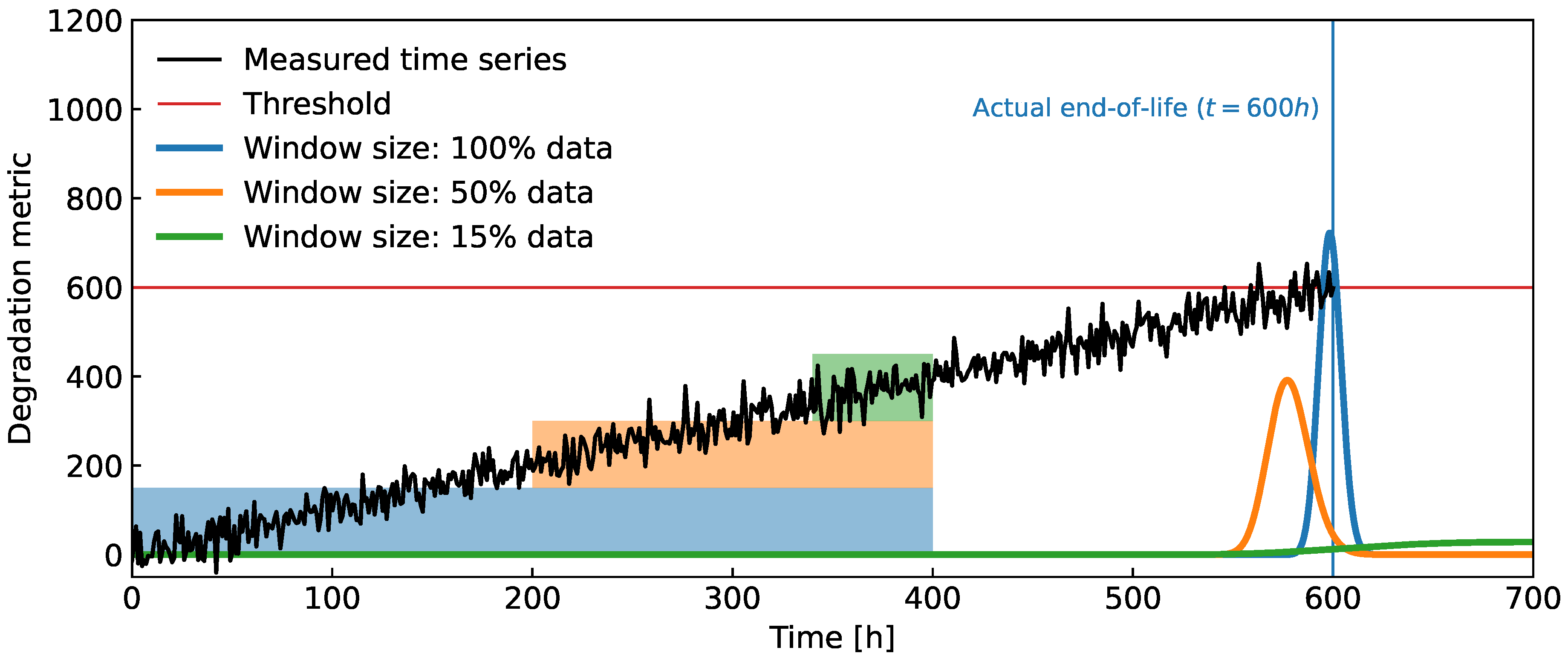
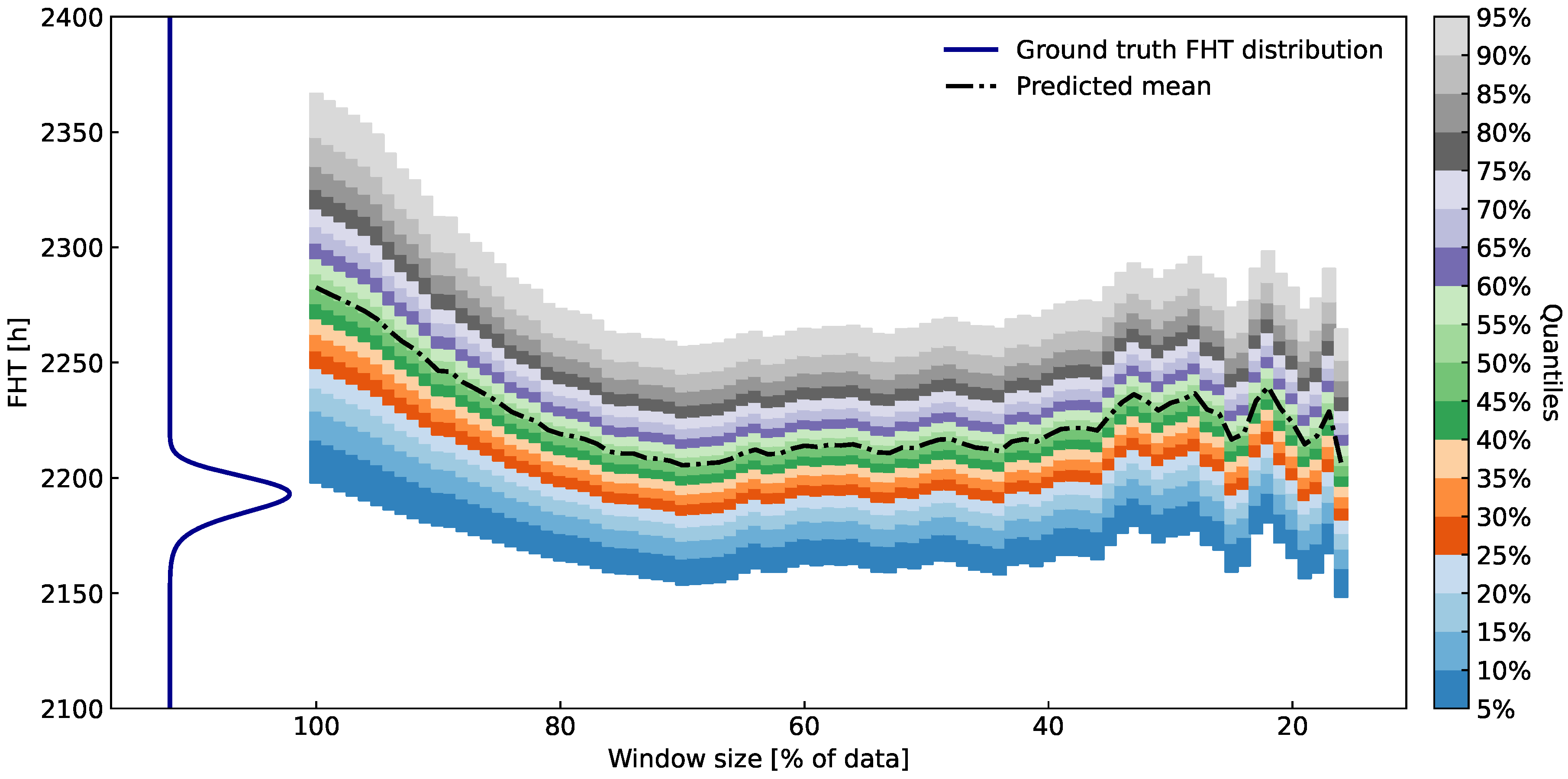
3.1. Case 1: Time Series with a Fixed Linear Trend

In this simplest case, the latent variable $x\left(t\right)$ exhibits a fixed linear trend, while the measured health indicator $y\left(t\right)$ is corrupted with noise

$$\begin{array}{c}\hfill x\left(t\right)=n+kt,n,k\in \mathbb{R}\left(\mathrm{Latent}\mathrm{health}\mathrm{indicator}\right),\end{array}$$

(17)

$$\begin{array}{c}\hfill y\left(t\right)=x\left(t\right)+\xi \left(t\right),\xi \sim \mathcal{N}(0,{\sigma }_{\xi }^2),{\sigma }_{\xi }\in {\mathbb{R}}^{+}\left(\mathrm{Observed}\mathrm{health}\mathrm{indicator}\right).\end{array}$$

(18)

The parameters used in the simulation are given in Table 1.

Table 1. Parameters of the linear trend model with fixed parameters (case 1).

Simulated Scenario	n	k	${\mathit{\sigma }}_{\mathit{\eta }}^2$	$\mathit{\alpha }$
Case 1	0	1	30	600

The simulated time series with a fixed linear trend is plotted in Figure 2. The time between consecutive samples is $t_{i+1}-t_i=1$ h. At time $t_N=400$ h several local linear trend models are estimated over data windows $M\in \{400,200,60\}$ and then used to evaluate the distribution of FHT. It is not surprising that utilizing all the available data provide the most accurate prediction of FHT.

Figure 2. Simulated time series with a fixed linear trend. The measured $y\left(t\right)$ are collected for 0 h $\le t\le 400$ h and the distributions of FHT are evaluated at t = 400 h for three different windows. The shortest window (green square) is [340 h, 400 h], which means the last $15\%$ of the available data, while the longest window (blue square) [0 h, 400 h] utilizes all of the available data. The remaining window (orange square) utilizes 50 % of the available data.

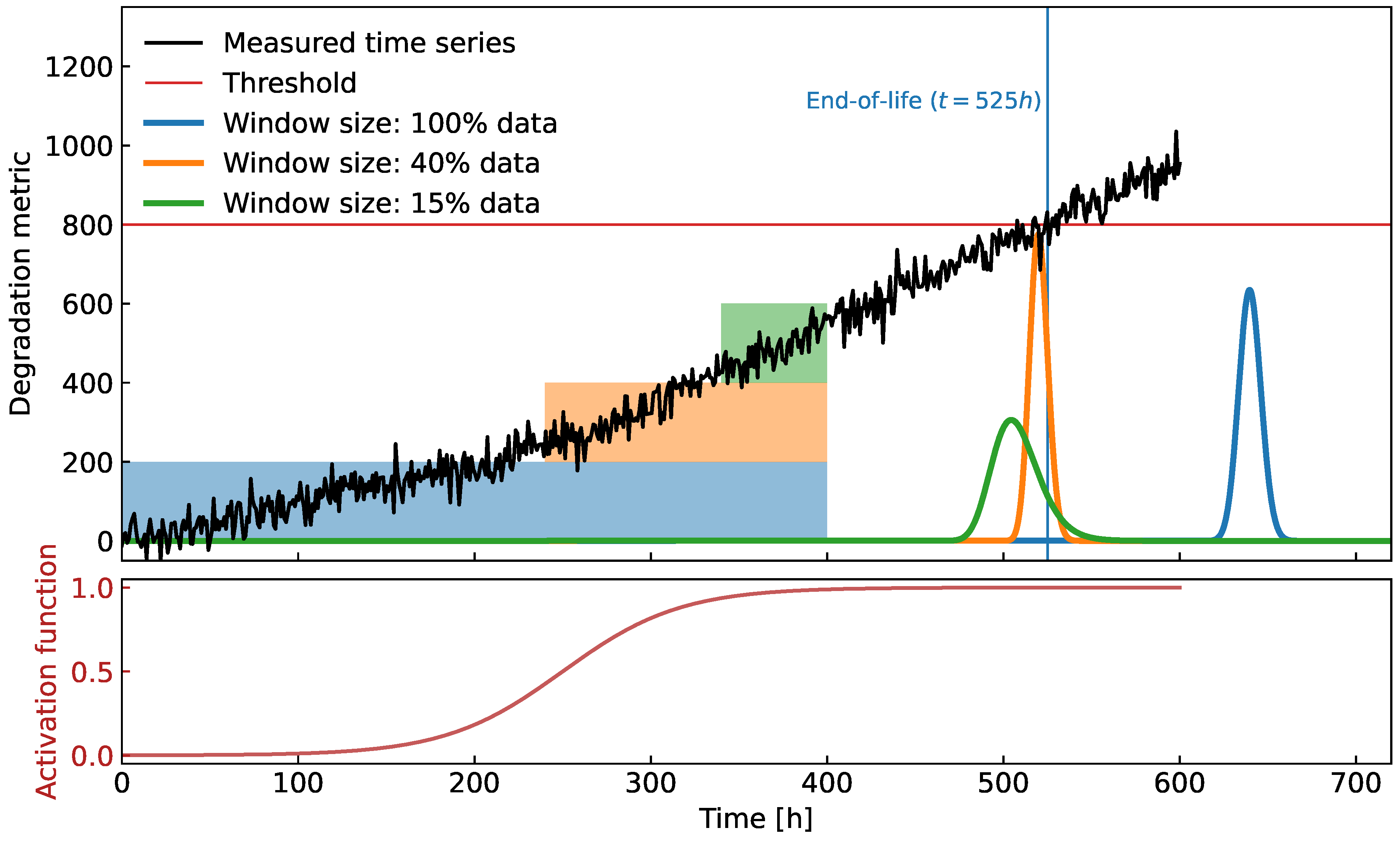
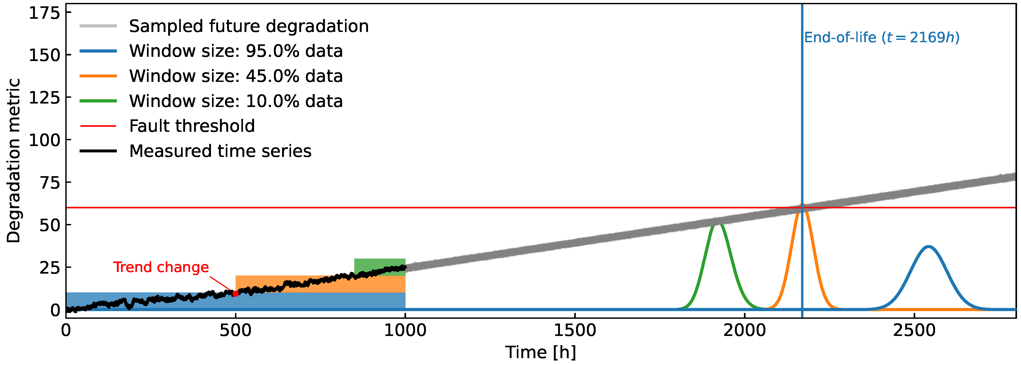
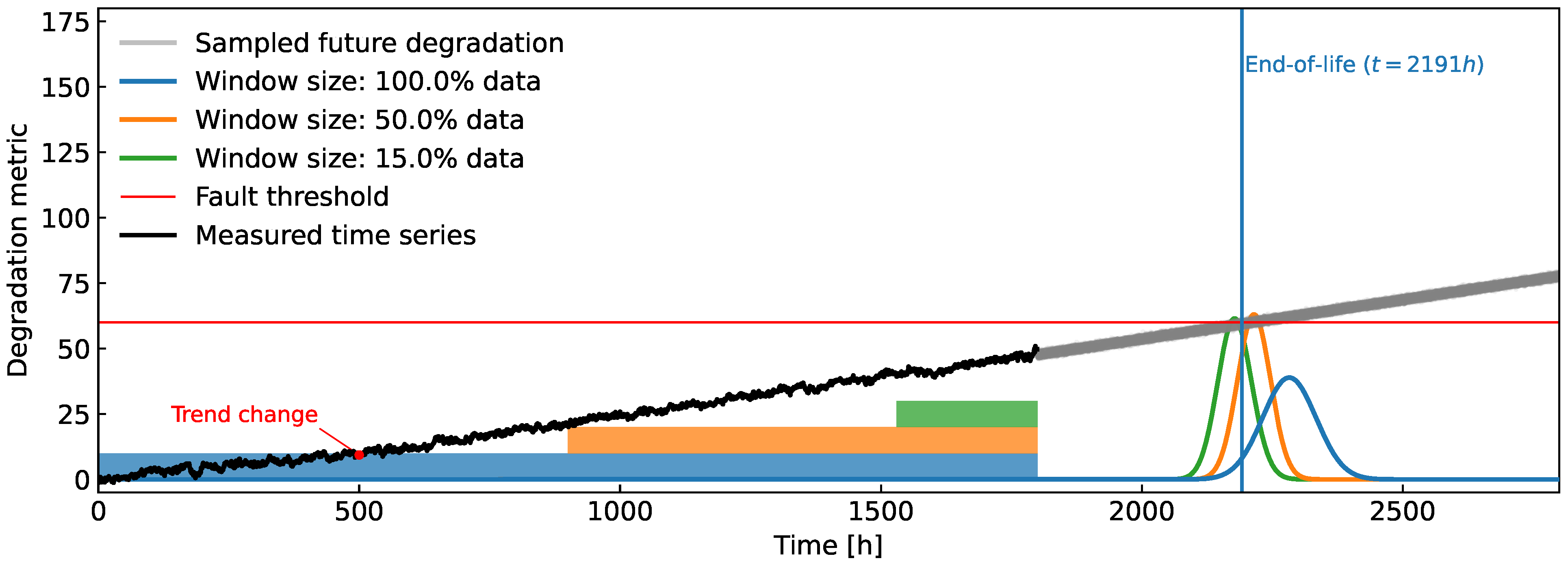
3.2. Case 2: Time Series with Linear Trend Subjected to Abrupt Changes

Like case 1, the latent variable follows a linear function, but its parameters undergo an abrupt change

$$\begin{array}{cc}\hfill x\left(t\right)& =\left(1-\varphi \left(t\right)\right)(k_{1}t+n_1)+\varphi \left(t\right)(k_{2}t+n_2),k_1,k_2,n_1,n_2\in \mathbb{R}(\mathrm{Latent}\mathrm{health}\mathrm{indicator}),\hfill \end{array}$$

(19)

$$\begin{array}{cc}\hfill \varphi \left(t\right)& =\frac{1}{1+exp\left(-\kappa (t-\tau )\right)},\kappa \in {\mathbb{R}}^{+},\tau \in \mathbb{R},\hfill \end{array}$$

(20)

$$\begin{array}{cc}\hfill n_2& =(k_1-k_2)\tau +n_1,\hfill \end{array}$$

(21)

$$\begin{array}{cc}\hfill y\left(t\right)& =x\left(t\right)+\xi \left(t\right),\xi \sim \mathcal{N}(0,{\sigma }_{\xi }^2),{\sigma }_{\xi }\in {\mathbb{R}}^{+}(\mathrm{Observed}\mathrm{health}\mathrm{indicator}),\hfill \end{array}$$

(22)

where $\varphi \left(t\right)$ is the sigmoid function which changes the system from $x\left(t\right)=k_{1}t+n_2$ to $x\left(t\right)=k_{2}t+n_2$. With the parameters $\tau$ and $\kappa$, one defines the time of transition and the rate of transition, respectively. Note that $n_2$ is not a free parameter to ensure a more natural-looking transition. The parameters used to simulate the second example are provided in Table 2.

Table 2. Parameters of the linear trend model with switching parameters (case 2).

Simulated Scenario	n	k	${\mathit{\sigma }}_{\mathit{\eta }}^2$	$\mathit{\tau }$ [h]	$\mathit{\alpha }$	$\mathit{\kappa }$ [h−1]
Case 2	$n_1=0$	$k_1=1$	30	250	800	$0.03$
	$n_2$ (calculated by (20)) = $-250$	$k_2=3$	30

In Figure 3, the simulated time series is presented along with the predicted distributions of the FHT obtained from local models estimated on three different data windows. Due to shifts in the trend, the forecasted FHT distribution from shorter windows proves more accurate than predictions derived from longer time windows. However, excessively brief windows are not advisable. The predictive quality diminishes as windows become too short, primarily due to heightened noise interference, particularly when the noise-to-signal ratio is high. In this specific case, we opted to show the predictions from window lengths that effectively highlight both the advantages and drawbacks of varying window durations.

Figure 3. (Top) Time series with an abrupt change in the linear trend and the distributions of the FHT obtained from local models evaluated over different data windows (15 % of available data–green square, 40 % of available data–orange square and full available data–blue square). Note that the trend model evaluated from the most recent data provides the most accurate prediction of the FHT. More specifically, in this case, utilizing only $40\%$ of the latest data yields the best result. (Bottom) The sigmoid function that switches between two linear trend models with different parameters.

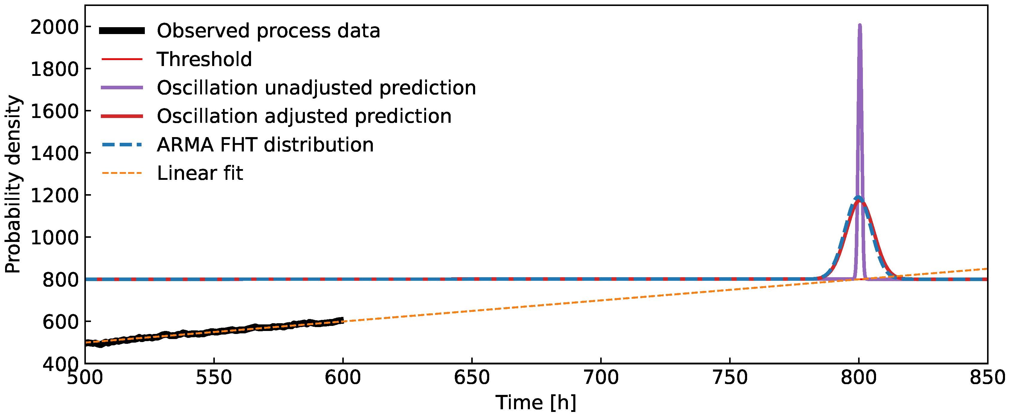
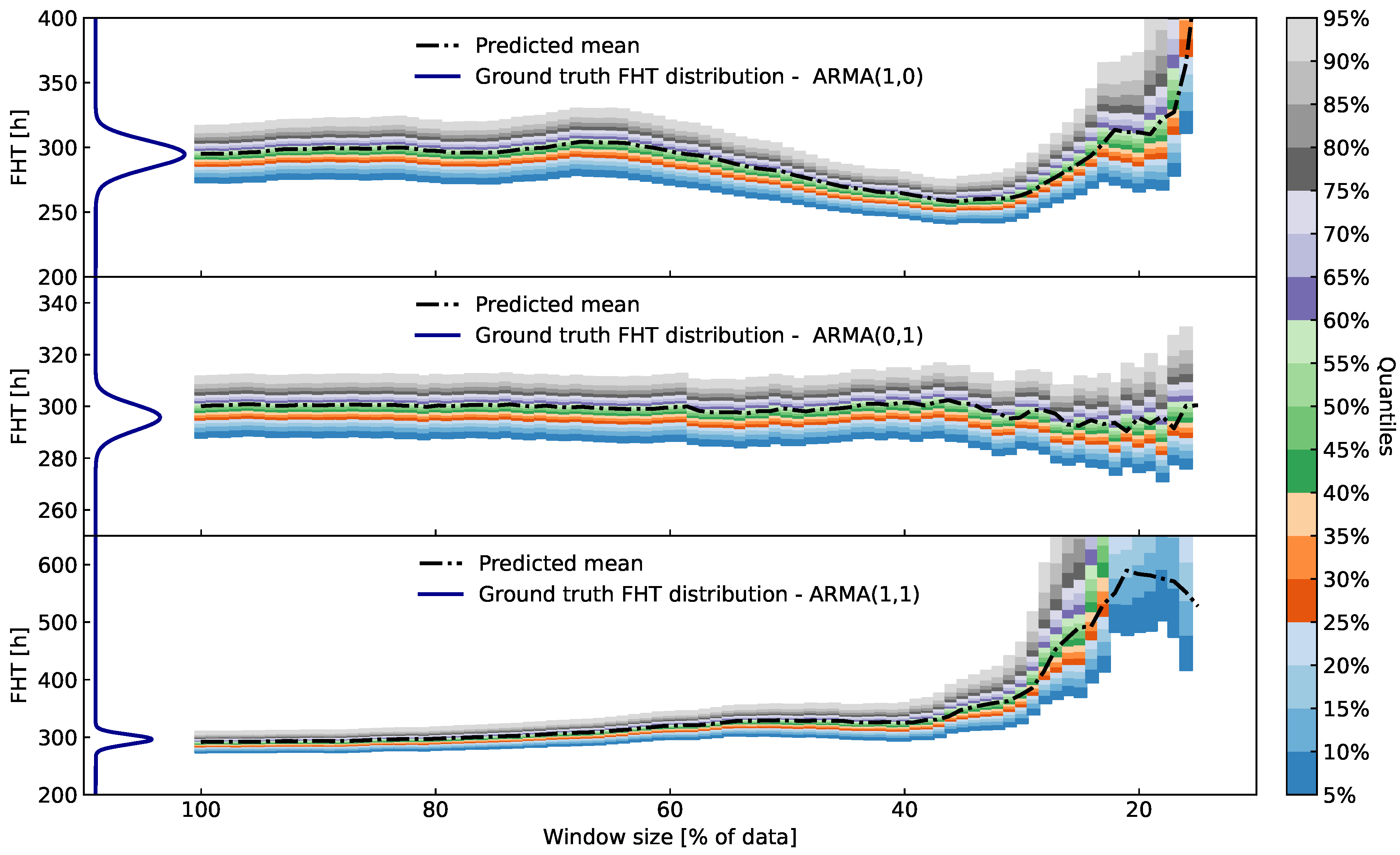
3.3. Case 3: Time Series Resulting from Arma Process with Fixed Parameters

A more general case of a time series containing a linear trend and an oscillatory component is analyzed $x\left(t\right)=x_{\mathrm{trend}}\left(t_j\right)+x_{\mathrm{osc}.}\left(t_j\right)$. For that purpose ARMA$(p,q)$ is utilized

$$\begin{array}{cc}\hfill x\left(t_j\right)& =x_{\mathrm{trend}}\left(t_j\right)+x_{\mathrm{osc}.}\left(t_j\right)(\mathrm{Latent}\mathrm{health}\mathrm{indicator}),\hfill \end{array}$$

(23)

$$\begin{array}{cc}\hfill x_{\mathrm{trend}}\left(t_j\right)& =l{t}_j+m,l,m\in \mathbb{R},\hfill \end{array}$$

(24)

$$\begin{array}{cc}\hfill x_{\mathrm{osc}.}\left(t_j\right)& =\sum _{i=1}^p{\varphi }_i{x}_{\mathrm{osc}.}\left(t_{j-i}\right)+\sum _{i=1}^q{\theta }_iϵ\left(t_{j-i}\right)+ϵ\left(t_j\right),ϵ\sim \mathcal{N}(0,{\sigma }_{ϵ}^2),{\varphi }_i,{\theta }_i\in \mathbb{R},{\sigma }_{ϵ}\in {\mathbb{R}}^{+},\hfill \end{array}$$

(25)

$$\begin{array}{cc}\hfill y\left(t_j\right)& =x\left(t_j\right)+\xi \left(t_j\right),\xi \left(t_j\right)\sim \mathcal{N}(0,{\sigma }_{\xi }^2),{\sigma }_{\xi }\in {\mathbb{R}}^{+}(\mathrm{Observed}\mathrm{health}\mathrm{indicator}).\hfill \end{array}$$

(26)

Following the same steps as in Section 3.1 yields FHT distributions that are too narrow since the oscillations of the latent variable are falsely regarded as white measurement noise. To circumvent this problem, we note that the scale of oscillations $\mathrm{E}\left[x_{\mathrm{osc}.}^2\right]$ is approximately the same as the scale of the perceived white noise ${\sigma }_{\eta }$. We can now transfer this perceived uncertainty, caused by oscillations, to the uncertainty of the threshold, so ${\sigma }_{\alpha }={\sigma }_{\eta }$ (see Equation (10)). Such an adaptation of the problem statement rescales the distribution of FHT to a much better width, as shown in Figure 4. Note that this approximation is meaningful only under conditions of relatively high signal-to-noise ratios. Otherwise, the uncertainty of the resulting FHT distributions may be overestimated. Alternatively, if the actual noise level ${\sigma }_{\xi }$ is known, one can subtract the actual noise level from the perceived white noise level, so ${\sigma }_{\alpha }=\sqrt{{\sigma }_{\eta }^2-{\sigma }_{\xi }^2}.$

Figure 4. Accounting for the variability in the internal variable by using the distribution of $\alpha$. The predictions rely on time series resulting from an ARMA process. The blue curve shows the ground truth, i.e., the prediction obtained with MC sampling of the latent model composed of a deterministic linear trend with ARMA $(1,0)$ oscillations, see Equation (23).

To adequately test the algorithm, three different ARMA models are employed to simulate oscillating latent variables. Their parameters are presented in Table 3.

Table 3. Parameters of ARMA models used to generate the time series.

Simulated Scenario	n	k	${\mathit{\sigma }}_{\mathit{\eta }}^2$	${\mathit{\sigma }}_{\mathit{\xi }}^2$	${\mathit{\varphi }}_1$	${\mathit{\theta }}_1$
ARMA $(1,0)$	0	1	5	5	$0.9$	0
ARMA $(0,1)$	0	1	5	5	0	$0.3$
ARMA $(1,1)$	0	1	5	5	$0.9$	$0.3$

Their typical behavior is showcased in Figure 5.

Figure 5. Time series generated by three different ARMA processes with the parameters given in Table 3.

In Figure 6, the algorithm was tested using three data windows of different sizes. For a meaningful comparison to the resulting distributions, the ground truth FHT distribution was approximated by MC sampling of the known ARMA process and compared to the results.

Figure 6. The distributions of FHT evaluated at time $t_N=200$ for three different ARMA models. With the full available training data at time $t_N=200$ presented in black for all three figures. Additionally, three different windows for estimation of the local trends are used: $[160,200]$ or the last $20\%$, $[120,200]$ or the last $60\%$ and $[0,200]$ or $100\%$ of the available data.

Examining the same situation from a different standpoint, Figure 7 features the same latent processes as Figure 6, but instead the quantiles of the resulting FHT distributions from various sizes of the data windows are presented.

Figure 7. Quantile plots over time for three different simulated processes (see Figure 6 for their time signals). The predicted FHT distributions calculated by the proposed algorithm stay in line with the ground truth when at least $2/3$ (from the start) of the data are taken into account. When data are taken at the beginning of the process (far from the FHT, e.g., the first $1/3$ of the dataset), the variance of the predicted distributions grows significantly, thus signaling an unreliable prognosis.

It turns out that with enough data and distance from the threshold, the algorithm stands as a viable alternative to a full regression of an ARMA model for FHT prediction. It is also worth noting that in this case, where the time series has a constant trend, retaining as much information as possible leads to more accurate predictions.

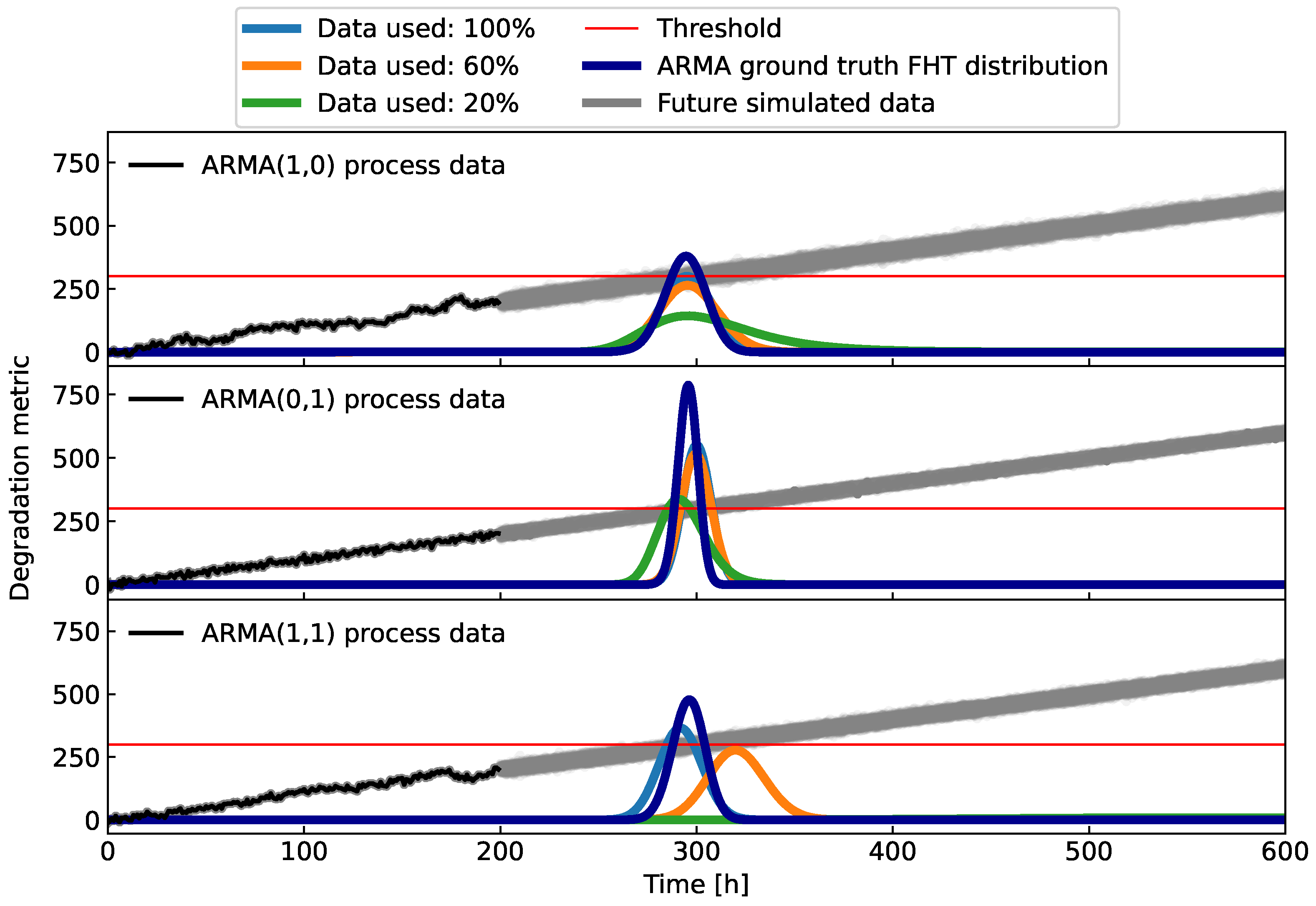
3.4. Case 4: Time Series Resulting from Arma Process with Abruptly Changing Parameters

In dynamical situations, an important feature of the prediction algorithm is the flexibility to quickly adapt to changes in trends. For that purpose, we again utilize limited-size time windows. Similarly to Section 3.2, the algorithm is tested on data generated by ARMA process featuring a change in the trend. The model parameters used for simulation are shown in Table 4.

Table 4. Parameters of the ARMA model with switching parameters.

Simulated Scenario	n	k	${\mathit{\sigma }}_{\mathit{\eta }}^2$	Time of Change [h]	$\mathit{\alpha }$
Case 4	$n_1=0$	$k_1=0.02$	$0.04$	500	60
	$n_2=-5$	$k_2=0.03$	$0.04$

In Figure 8 and Figure 9, the simulated ARMA process with a change in trend is depicted for two examples. The first example has the data from $t=[0,1000]$ h available and for the second one, we use $t=[0,1800]$ h. The change in trend is initiated around $t=500$ h for both examples. For the data interval up to about $t=500$ h, the slope of the trend is $0.02$, which changes to $0.03$ afterward. The resulting FHT distributions derived from different data windows are illustrated in Figure 8 and Figure 9. An obvious improvement in the quality of prognosis can be observed after incorporating only the data after the trend change.

Figure 8. Synthetic experiment on the ARMA time signal with an abrupt change in the trend (around $t=500$ h). Data, available for the prognosis, were limited up to $t=1000$ h. Actual EOL is compared to results from the developed algorithm with various amounts of data taken into account, namely $10\%$ (green square), $45\%$ (orange square)and $95\%$ of the available data (blue square).

Figure 9. Second example of synthetic time signals of the ARMA process with an abrupt change in the trend (around $t=500$ h). The FHT distributions are derived with various amounts of data taken into account, namely $15\%$ (green square), $50\%$ (orange square) and all of the available data (blue square). Relating to Figure 8, there were more available data for the prognostic algorithm here, up to $t=1800$ h. But on the other hand, EOL is now much closer and any large oscillations in time signal will importantly affect the actual breach of the threshold.

In Figure 10 and Figure 11, we show quantiles of FHT distributions from local trend models obtained from differently sized windows on the data. For example, a window $[800,1000]$ h includes $20\%$ of the data up to 1000 h. The consequence of such flexibility can be seen in frequent changes in the mean of the FHT distribution acquired from the most recent data, where the trend is not yet obvious. For comparison, ground truth FHT distribution (dark blue curve) is also provided.

Figure 10. Quantiles of FHT distributions over various percentages of available data at $t=1000$ h taken into account. The artificial data are from an ARMA process with a change in the trend. On the left, ground truth FHT is presented (dark blue curve). The prediction is best when taking at most $50\%$ of the recent data since that is when the trend change has occurred.

Figure 11. Quantiles of FHT distributions over various percentages of available data at $t=1800$ h taken into account. The artificial data are from an ARMA process with a change in the trend. On the left, ground truth FHT is presented (dark blue curve). The prediction improves when taking up at most $60\%$ of the recent data. Since the time of prediction is relatively close to the EOL, there is a noticeable difference between the bias and the variance in the ground truth and the predictive FHT distribution.

We notice that up to the point, adding data improves precision and accuracy. If we also include data before the trend change, the precision of the predictions does not suffer as much as the accuracy. This highlights a potential limitation in assessing the reliability of the prediction. Without the variance in the prediction ballooning, this could lead to a false sense of confidence in the prediction by the operator.

We also notice a slight bias in predictions when the time of prediction is somewhat close to the EOL; see Figure 9. Due to the limited time available, any large enough oscillation significantly impacts the point of threshold crossing. The latent variable is therefore unable to regress to the mean before the crossing, which significantly alters the ground truth distribution.

4. Application to the Prognosis of a Laboratory Sofc System

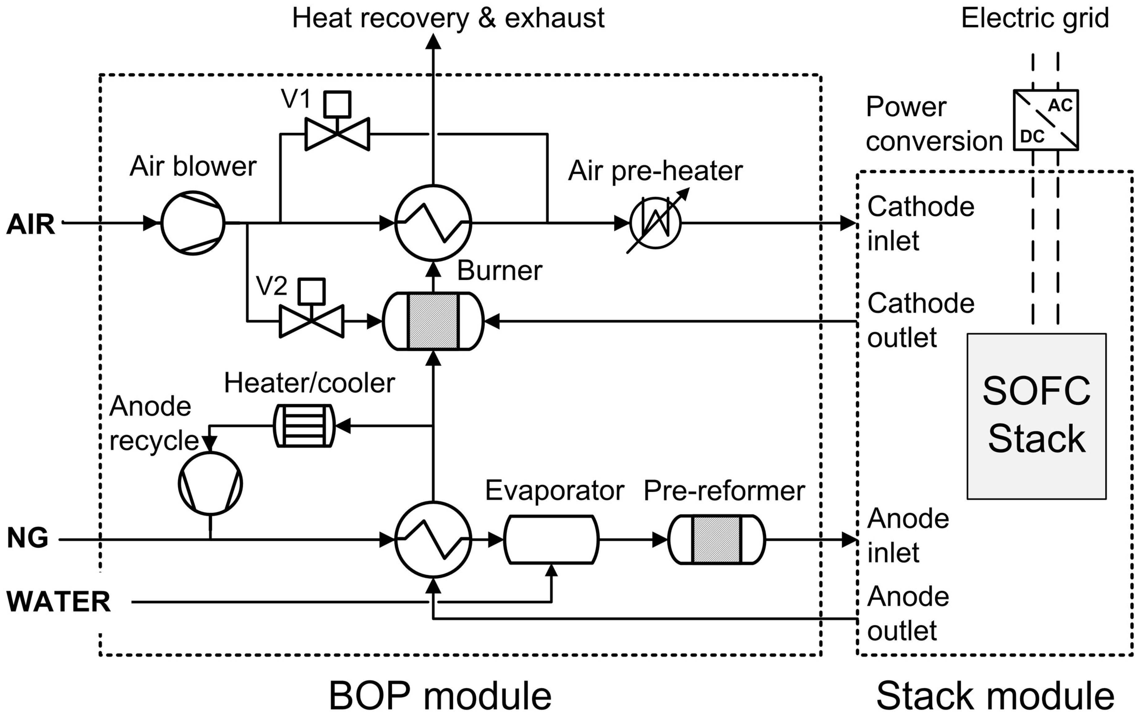
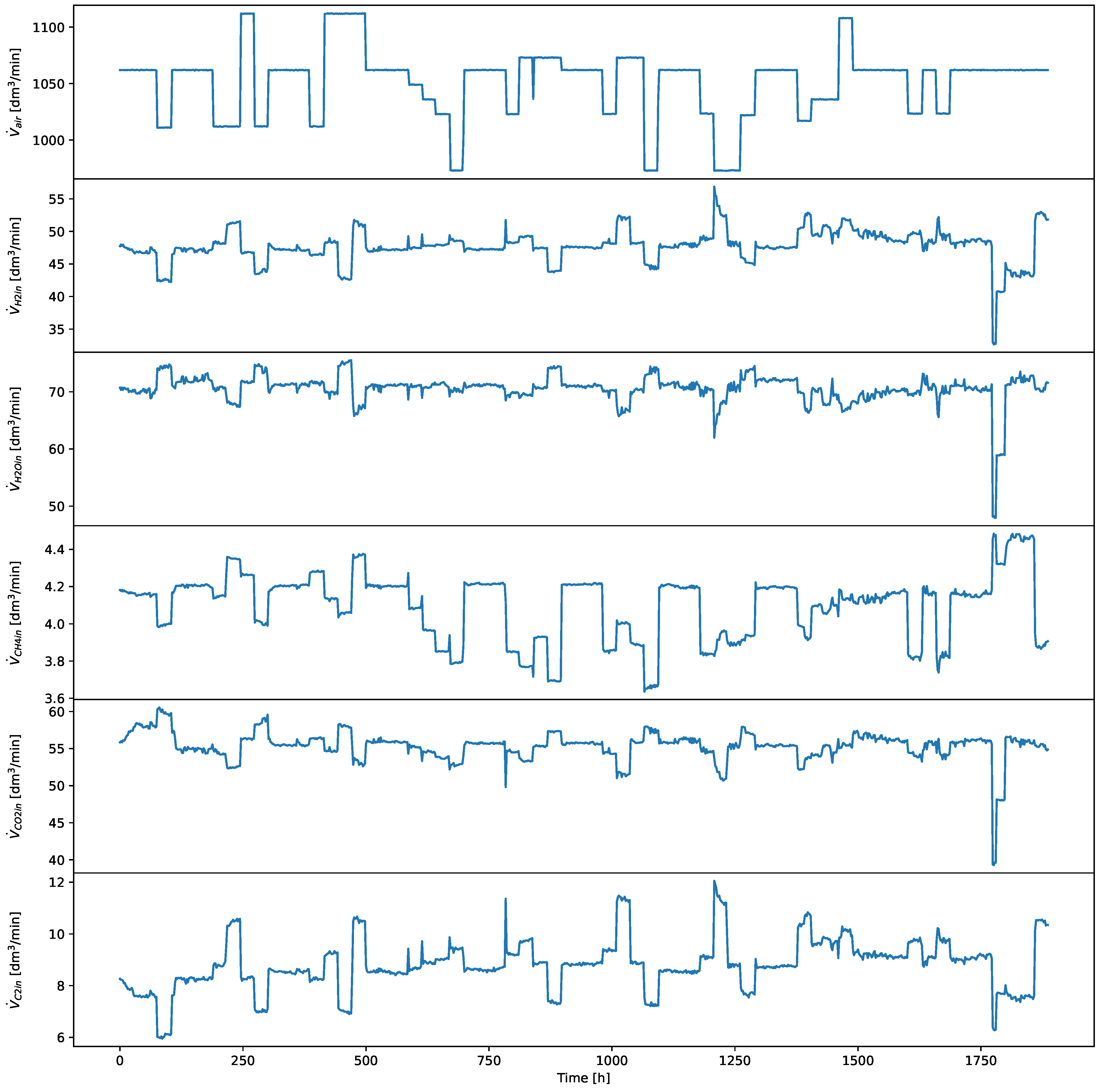
4.1. System Description

The study was conducted on a 10kW SOFC system, which consists of two interconnected modules, the balance of plant (BoP) and the stack. The layout of the system can be seen in Figure 12. It utilizes a single, planar, 80-cell SOFC stack powered by methane.

Figure 12. The layout of the 10kW SOFC system used for experimental validation.

Water–gas shift (WGS), steam methane reforming (SMR) and hydrogen-oxidation reactions take place inside to produce heat, water and electrical power. Air is fed by the blower to the cathode inlet of the stack. Methane is passed through a reformer in order to obtain hydrogen, which is then delivered to the anode inlet. The remaining fuel in the cathode output is recycled. During the test, various operational parameters were manipulated for a complete characterization of the system.

4.2. Lumped Model of the Stack

The model of the stack is based on its energy balance [3]

$${\mathrm{K}}_{\mathrm{s}}\frac{d{T}_{\mathrm{out}}}{dt}={\dot{E}}_{\mathrm{in}}\left(T_{\mathrm{in}}\right)-{\dot{E}}_{\mathrm{out}}\left(T_{\mathrm{out}}\right)-IU\left(T_{\mathrm{out}}\right),$$

(27)

where $T_{\mathrm{out}}$ and $T_{\mathrm{in}}$ are the outlet and inlet gas temperatures, ${\dot{E}}_{\mathrm{in}}$ and ${\dot{E}}_{\mathrm{out}}$ denote energy flows in and out of the stack, ${\mathrm{K}}_{\mathrm{s}}$ denotes lumped heat capacity of the stack, U is stack voltage and I is load current.

The inlet/outlet energy flows $\dot{E}$ are defined as [3]

$${\dot{E}}_{\xi }=\sum _i{\dot{n}}_i^{\xi }{h}_i\left(T^{\xi }\right),$$

(28)

where ${\dot{n}}_i^{\xi }$ denotes the molar flow of the $i^{\mathrm{th}}$ gas component, i ∈ {H₂, H₂O, CH₄, CO, CO₂, O₂, N₂}, at corresponding locations where $\xi \in \{\mathrm{in},\mathrm{out}\}$, i.e., stack inlet/outlet, and corresponding temperatures $T_i^{\xi }$. $h_i$ is the enthalpy of the gas.

For the purpose of constructing such a simple model, SMR, WGS and hydrogen oxidation reactions are considered to be in thermodynamic equilibrium. This assumption is often employed in SOFC systems and can be justified [3,22,23,24,25]. Assuming total methane reforming and using the WGS equilibrium constant from [26], the reforming equilibrium can be solved [27], yielding the concentration of each outlet gas component, which we take to be proportional to its flow rates.

The stack voltage U can be expressed as

$$U={\mathrm{N}}_0\left(U_0-\mathrm{ASR}\times \frac{I}{\mathrm{A}}\right),$$

(29)

where A is the active area of a single cell, ${\mathrm{N}}_0$ is the number of cells and $U_0$ is the Nernst voltage [28], p. 269

$$\begin{array}{c}\hfill U_0=1.2586-0.000252T+\frac{\mathrm{R}T}{2\mathrm{F}}ln\frac{p_{{\mathrm{H}}_2}{p}_{{\mathrm{O}}_2}^{0.5}}{p_{{\mathrm{H}}_2\mathrm{O}}},\end{array}$$

(30)

where R is the universal gas constant.

For an approximation of the partial pressure of gases inside the stack, the average of input and output molar flows is used

$$\begin{array}{c}\hfill p_j=\frac{1}{2}\left(\frac{{\dot{n}}_j^{\mathrm{in}}}{{\dot{n}}_{\mathrm{tot}.}^{\mathrm{in}}}+\frac{{\dot{n}}_j^{\mathrm{out}}}{{\dot{n}}_{\mathrm{tot}.}^{\mathrm{out}}}\right),\end{array}$$

(31)

where $j\in \left\{{\mathrm{H}}_2,{\mathrm{H}}_2\mathrm{O},{\mathrm{O}}_2\right\}$ and ${\dot{n}}_{\mathrm{tot}.}^{\mathrm{in}/\mathrm{out}}$ are total anode or cathode inlet/outlet molar flows.

The temperature variation of lumped Ohmic ASR of a single cell can be expressed by the second-order Steinhart–Hart equation [23,28]

$$\mathrm{ASR}={\mathrm{ASR}}_{0}exp\left[\frac{30000}{\mathrm{R}}\left(\frac{1}{T}-\frac{1}{T_0}\right)\right],$$

(32)

where ${\mathrm{ASR}}_0$ is ASR at reference temperature $T_0$. It is ${\mathrm{ASR}}_0$ we are actually after, since we are in a need of temperature-invariant health index.

Putting all the necessary parts together, we arrive at the full lumped dynamic model of the stack:

$$\begin{array}{c}\hfill \begin{array}{cc}\hfill {\mathrm{K}}_{\mathrm{s}}\frac{dT}{dt}& ={\dot{E}}_{\mathrm{in}}\left(T_{\mathrm{in}}\right)-{\dot{E}}_{\mathrm{out}}\left(T\right)\hfill \\ \hfill & -I{\mathrm{N}}_0\left(1.2586-0.000252T+\frac{\mathrm{R}T}{2\mathrm{F}}ln\frac{p_{{\mathrm{H}}_2}{p}_{{\mathrm{O}}_2}^{0.5}}{p_{{\mathrm{H}}_2\mathrm{O}}}-{\mathrm{ASR}}_{0}exp\left[\frac{30000}{\mathrm{R}}\left(\frac{1}{T}-\frac{1}{T_0}\right)\right]\times \frac{I}{\mathrm{A}}\right).\hfill \end{array}\end{array}$$

(33)

Since it was only possible to measure ${\mathrm{ASR}}_0$ indirectly, and (33) is non-linear, an unscented Kalman filter [29], highly suitable to such problems, was used to filter out as much noise from the measurements as possible.

Lastly, an adequate criterion for the EOL for the stack is needed. While we will be using some rather arbitrary value of ${\mathrm{ASR}}_0$ that signals the EOL to obtain a physically meaningful value, one needs to define the lowest appropriate stack voltage at the same typical operating point. This minimum voltage can be easily converted to an ${\mathrm{ASR}}_0$ value using (29).

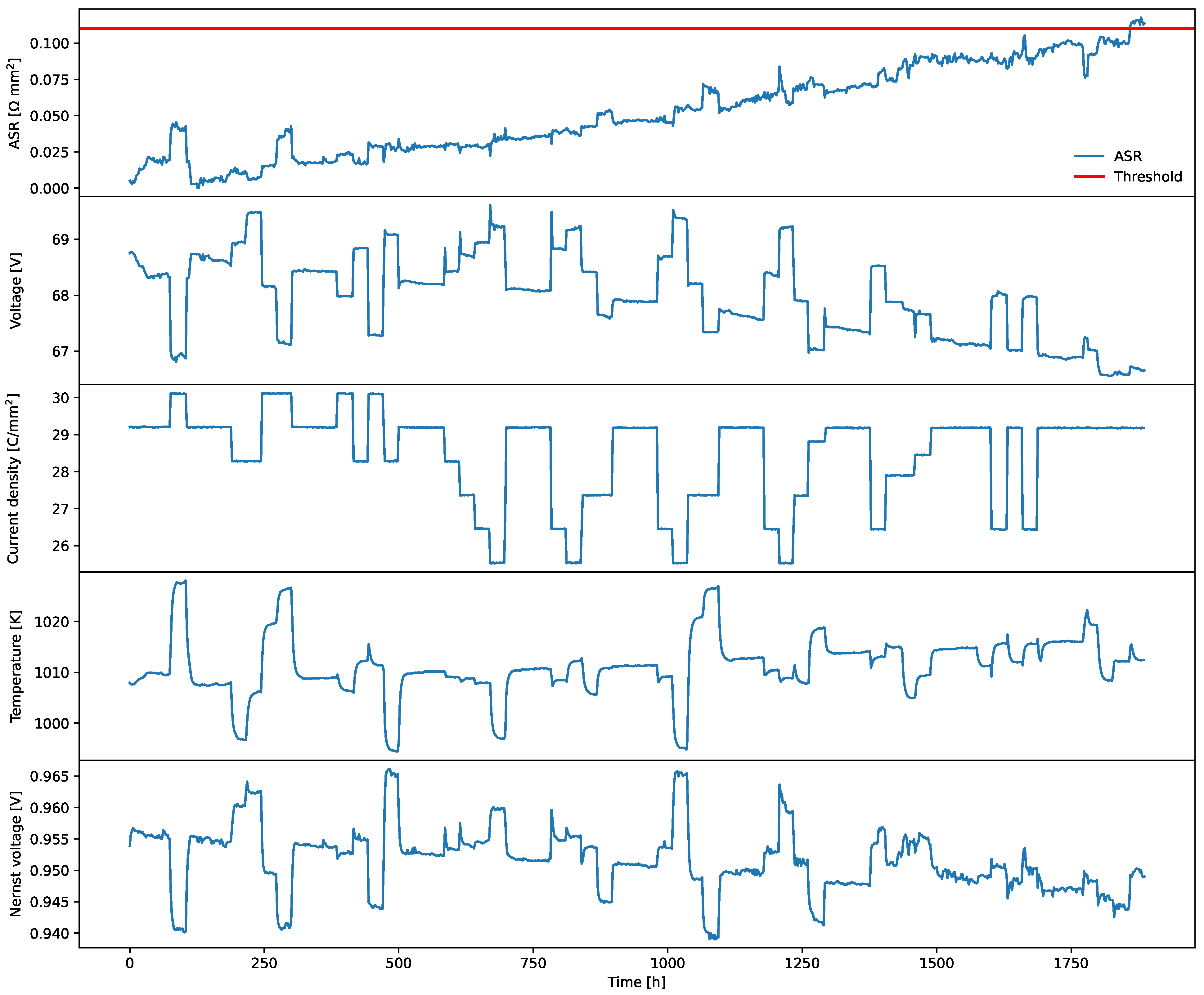
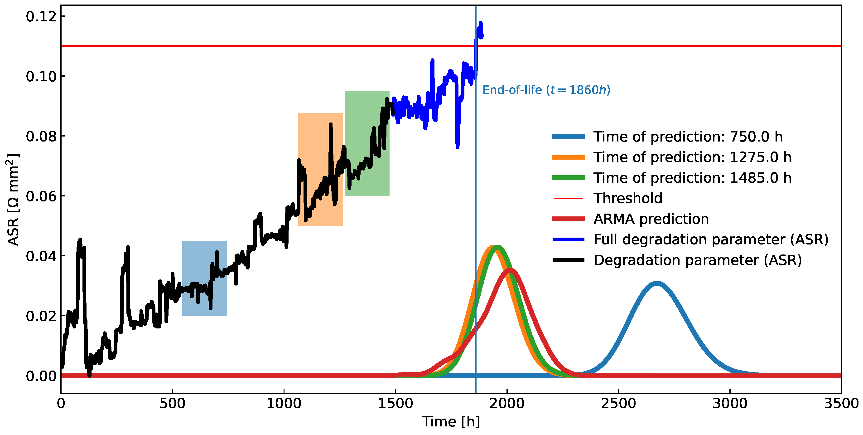
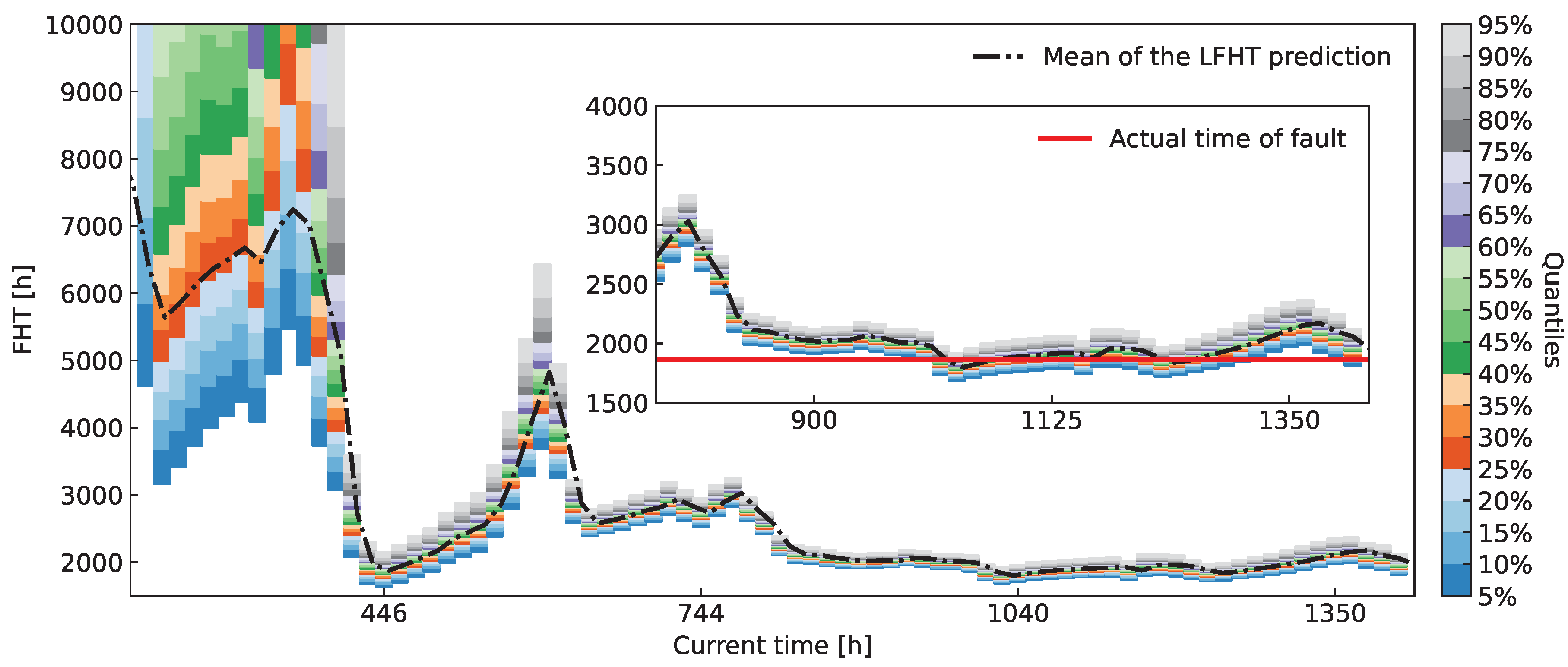
4.3. Prognostics of the Remaining Useful Life Based on ASR as a Health Indicator

In Figure 13 and Figure 14, operational data of almost 1850h are presented. The system was operated in a non-stationary regime during which there were frequent changes in the load. Therefore, the stack voltage is not the best candidate for the health indicator. Instead, ASR was chosen as the health metric since it is invariant to changes in process variables (technically, we have chosen ASR₀ as the metric according to (33)). For validation of the algorithm the threshold of ASR was set to $0.11\Omega$mm² (a red horizontal line in Figure 13).

Figure 13. Data from SOFC stack experiment in [12]. From top to bottom: ASR, stack voltage, current density, outlet temperature and Nernst voltage.

Figure 14. Inflow data from SOFC stack experiment in [12]. From top to bottom: Air, H₂, H₂O, CH₄, CO₂, C₂ flows.

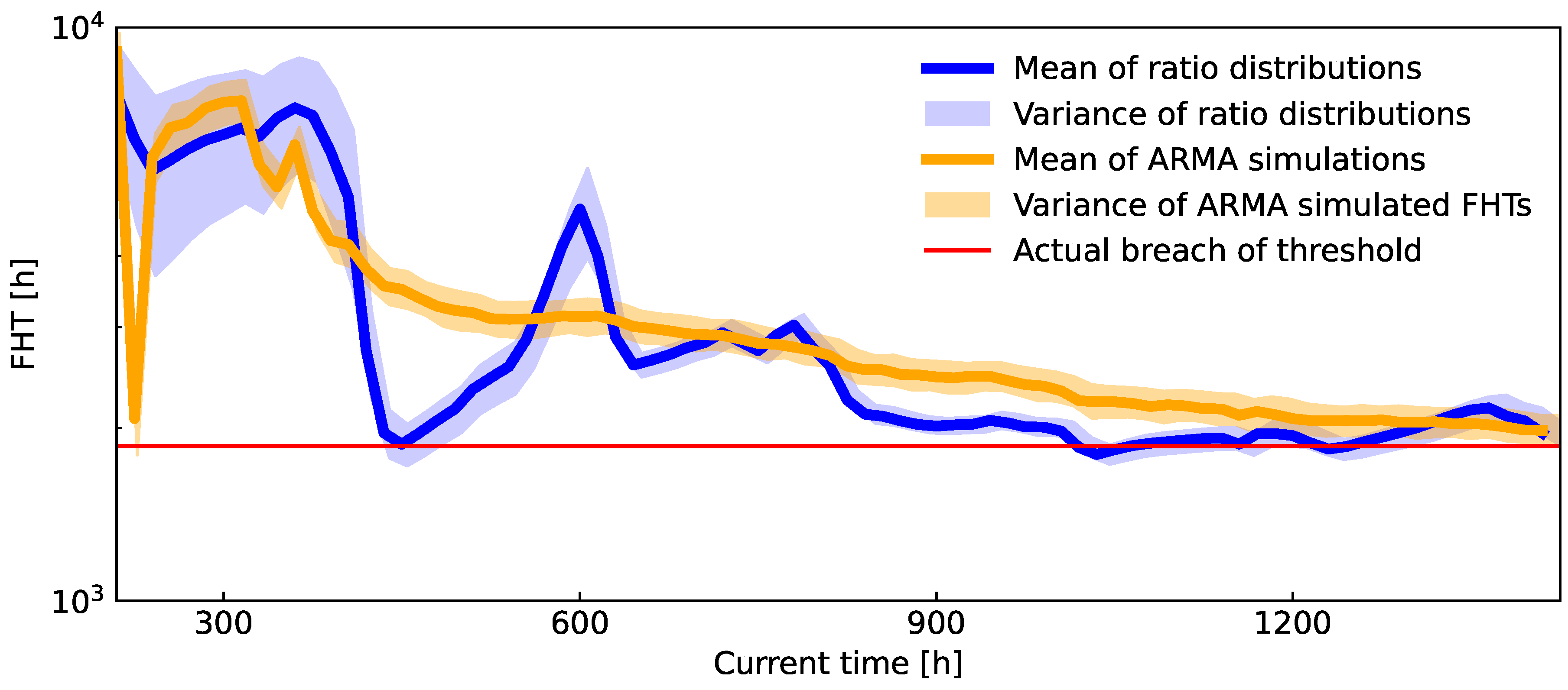
Validation of the Proposed Method by Comparison to an Alternative Prognostic Algorithm

To assess the new algorithm on experimental data, where the latent model is unknown, we decided to compare it to an ARMA process whose parameters were obtained by the maximum likelihood method. Specifically, we have used statsmodels v0.14.1 [30], a Python package for inference for statistical models. After comparing several different variations in the model via the Akaike information criterion, we have landed on ARMA $(2,0)$ with a deterministic linear function as an exogenous variable (same framework as in (23)).

4.4. Results

Results of the experimental data can be seen in Figure 15. The improvement in the quality of resulting FHT distribution is proportional to the number of data points included in the prognosis, which is expected since the ASR time signal includes no obvious trend changes. The alternative FHT distribution, sampled from fitted ARMA model, can be seen in Figure 15 as well. It was smoothed using kernel density estimation (KDE) [31] for easier comparison.

Figure 15. A demonstration of the application of the new algorithm on real-life ASR measurements. A major chunk of the data is used for learning (black curve), while the minor chunk is used for validation (dark blue curve). Few data windows, shown as rectangular colored windows (blue is the data window used for prediction at $t=750$ h, orange at $t=1275$ h and green at $t=1485$ h), were used on the learning part of the data to derive FHT predictions. The figure includes a comparison to an alternative prognostic algorithm, an ARMA process, fitted on the whole learning part of the data, which obtains similar results.

To further compare the quality of the derived algorithm to an ARMA model, Figure 16 shows the evolution of variance and mean of both predictive distributions over the amount of data taken into account. The time of perceived EOL is shown with a horizontal red line.

Figure 16. Comparison of ARMA and the derived prognostic algorithm on the experimental data. The x-axis represents the percentage of the full set of data used, simulating the real-life scenario of data accumulating over time. The horizontal red line denotes EOL for the stack. While both models converge to a similar solution, which is in line with the actual ASR’s breach of threshold when at least $2/3$ of data are available, they both experience major deviations from the correct result when the data are insufficient. The major difference between the methods is that the new prognostic algorithm undergoes variance explosion when data are scarce, while ARMA stays overconfident.

Again, the presented algorithm shows comparable results to the alternative. The larger variance at the start can be attributed to the lack of sufficient data. Such uncertainty in the prediction can be valuable for the operator, as it suggests a need for caution when interpreting the prognosis. Over time we can observe a slow regression of the mean to the ground truth FHT, together with the variance shrinking to a useful level.

On the other hand, the alternative prediction from an ARMA model suffers from overconfidence issues in the beginning, since only a point-wise fit is considered for the parameters. Other than that, it also slowly converges to the vicinity of the actual FHT.

Similarly to Figure 16, Figure 17 shows quantiles of FHT distributions derived throughout the experiment. Abrupt changes in the mean of the FHT distributions can be observed, which indicate volatile oscillations of ASR during the measurement process. In the magnified inset of the figure we again compare the actual FHT to the prediction. Upon closer examination, we conclude that the predicted FHT distributions successfully encompass the eventual EOL as early as $t=800$ h.

Figure 17. Quantile plot over time for ASR. The figure depicts the evolution of the FHT distribution over time, starting at 15% of the data and progressing to the full dataset. It simulates a real-life application where data comes in over time and the prognostic capabilities improve. The inset highlights the latter part of the measurement process, where the predicted FHT distribution can be trusted to assess the probable EOL.

5. Conclusions

In this paper, a novel algorithm for predicting the remaining useful life for SOFC systems based on adaptive trend estimation of the time-evolving health indicator is proposed. A distinctive feature of the algorithm is that the predicted distribution of the remaining useful life is provided in a closed form. Hence, the computational time is insignificant, thus rendering the algorithm appropriate for implementation in industrial low-cost platforms with limited computational resources.

The performance of the algorithm is first demonstrated on four different artificial types of time series that are intended to mimic the potential evolutions of the health indicators met in practice.

The study shows that in the simple case of a constant trend time series larger size data windows deliver more accurate predictions of FHT. If, on the other hand, the time series exhibits variable trends, shorter data windows offer better flexibility to account for the variations.

Tests on time series that depart from the strongly monotone features due to internal dynamics modeled by ARMA process show that the proposed algorithm consistently captures the distribution of FHT without the need for inferring the coefficients of the ARMA process.

Finally, the performance of the proposed algorithm is compared with a more elaborated algorithm ARMA $(2,0)$ on experimental data. Specifically, ASR measurements from a laboratory SOFC stack were modeled as a time series. It turns out that the proposed algorithm consistently delivers the same level of quality of prognosis throughout the experiment even though estimation of ARMA model parameters is computationally more demanding than operating with linear local trend.

To sum up, the proposed prognostic algorithm is usable as a plug-and-play tool appropriate for SOFC applications lacking specific prognostic models and without prior knowledge of the degradation. In the follow-up, it would be of interest to explore adaptive strategies to dynamically adjust the threshold values based on evolving system conditions. This adaptability could enhance the algorithm’s performance in handling varying degradation patterns and unexpected changes in the health indicator.

References

- Peng, J.; Huang, J.; Wu, X.; Xu, Y.; Chen, H.; Li, X. Solid oxide fuel cell (SOFC) performance evaluation, fault diagnosis and health control: A review. J. Power Sources 2021, 505, 230058. [Google Scholar] [CrossRef]
- Nakajo, A.; Tanasini, P.; Diethelm, S.; herle, J.V.; Favrat, D. Electrochemical model of solid oxide fuel cell for simulation at the stack scale II: Implementation of degradation processes. J. Electrochem. Soc. 2011, 158, B1102–B1118. [Google Scholar] [CrossRef]
- Marra, D.; Sorrentino, M.; Pohjoranta, A.; Pianese, C.; Kiviaho, J. A Lumped Dynamic Modelling Approach for Model-Based Control and Diagnosis of Solid Oxide Fuel Cell System with Anode Off-Gas Recycling. ECS Trans. 2015, 68, 3095. [Google Scholar] [CrossRef]
- Zhao, J.; Feng, X.; Pang, Q.; Wang, J.; Lian, Y.; Ouyang, M.; Burke, A.F. Battery prognostics and health management from a machine learning perspective. J. Power Sources 2023, 581, 233474. [Google Scholar] [CrossRef]
- Zhang, Y.; Tang, Q.; Zhang, Y.; Wang, J.; Stimming, U.; Lee, A.A. Identifying degradation patterns of lithium ion batteries from impedance spectroscopy using machine learning. Nat. Commun. 2020, 11, 1706. [Google Scholar] [CrossRef] [PubMed]
- Liu, H.; Chen, J.; Hissel, D.; Lu, J.; Hou, M.; Shao, Z. Prognostics methods and degradation indexes of proton exchange membrane fuel cells: A review. Renew. Sustain. Energy Rev. 2020, 123, 109721. [Google Scholar] [CrossRef]
- Ming, W.; Sun, P.; Zhang, Z.; Qiu, W.; Du, J.; Li, X.; Zhang, Y.; Zhang, G.; Liu, K.; Wang, Y.; et al. A systematic review of machine learning methods applied to fuel cells in performance evaluation, durability prediction, and application monitoring. Int. J. Hydrogen Energy 2023, 48, 5197–5228. [Google Scholar] [CrossRef]
- Marra, D.; Sorrentino, M.; Pianese, C.; Iwanschitz, B. A neural network estimator of solid oxide fuel cell performance for on-field diagnostics and prognostics applications. J. Power Sources 2013, 241, 320–329. [Google Scholar] [CrossRef]
- Wu, X.; Ye, Q. Fault diagnosis and prognostic of solid oxide fuel cells. J. Power Sources 2016, 321, 47–56. [Google Scholar] [CrossRef]
- Cheng, S.J.; Li, W.K.; Chang, T.J.; Hsu, C.H. Data-Driven Prognostics of the SOFC System Based on Dynamic Neural Network Models. Energies 2021, 14, 5841. [Google Scholar] [CrossRef]
- Zhang, X.; He, Z.; Zhan, Z.; Han, T. Performance degradation analysis and fault prognostics of solid oxide fuel cells using the data-driven method. Int. J. Hydrogen Energy 2021, 46, 18511–18523. [Google Scholar] [CrossRef]
- Dolenc, B.; Boškoski, P.; Pohjoranta, A.; Noponen, M.; Juričić, Đ. Hybrid Approach to Remaining Useful Life Prediction of Solid Oxide Fuel Cell Stack. ECS Trans. 2017, 78, 2251. [Google Scholar] [CrossRef]
- Cui, L.; Huo, H.; Xie, G.; Xu, J.; Kuang, X.; Dong, Z. Long-Term Degradation Trend Prediction and Remaining Useful Life Estimation for Solid Oxide Fuel Cells. Sustainability 2022, 14, 9069. [Google Scholar] [CrossRef]
- Dolenc, B.; Juričić, D.; Boškoski, P. Identification of the coupling functions between the process and the degradation dynamics by means of the variational Bayesian inference: An application to the solid-oxide fuel cells. Philos. Trans. R. Soc. A Math. Phys. Eng. Sci. 2019, 377, 20190086. [Google Scholar] [CrossRef] [PubMed]
- Xu, Y.; Jiang, C.; Peng, J.; Wu, X.L.; Xiao, L.; Li, X. Fault Prognosis Method for Solid Oxide Fuel Cells Based on Mechanism Degradation Process Model and Particle Filtering. IEEE Trans. Power Electron. 2023, 38, 6831–6840. [Google Scholar] [CrossRef]
- Polverino, P.; Gallo, M.; Pianese, C. Development of mathematical transfer functions correlating Solid Oxide Fuel Cell degradation to operating conditions for Accelerated Stress Test protocols design. J. Power Sources 2021, 491, 229521. [Google Scholar] [CrossRef]
- Guida, M.; Postiglione, F.; Pulcini, G. A random-effects model for long-term degradation analysis of solid oxide fuel cells. Reliab. Eng. Syst. Saf. 2015, 140, 88–98. [Google Scholar] [CrossRef]
- Naeini, M.; Cotton, J.S.; Adams, T.A. An eco-technoeconomic analysis of hydrogen production using solid oxide electrolysis cells that accounts for long-term degradation. Front. Energy Res. 2022, 10, 1015465. [Google Scholar] [CrossRef]
- Goldberger, A.; Shenhart, W.; Wilks, S. Econometric Theory; Wiley Series In Probability and Statistics: Applied Probability and Statist Ics Section Series; John Wiley & Sons: New York, NY, USA, 1964. [Google Scholar]
- Simon, M.K. Probability Distributions Involving Gaussian Random Variables: A Handbook for Engineers and Scientists; International Series in Engineering and Computer Science; Springer: New York, NY, USA, 2007. [Google Scholar]
- Shumway, R.H.; Stoffer, D.S. ARIMA Models. In Time Series Analysis and Its Applications: With R Examples; Springer International Publishing: Cham, Switzerland, 2017; pp. 75–163. [Google Scholar] [CrossRef]
- Aguiar, P.; Adjiman, C.S.; Brandon, N.P. Anode-supported intermediate temperature direct internal reforming solid oxide fuel cell. I: Model-based steady-state performance. J. Power Sources 2004, 138, 120–136. [Google Scholar] [CrossRef]
- Marra, D.; Pianese, C.; Polverino, P.; Sorrentino, M. Models Hierarchy; Springer: Berlin/Heidelberg, Germany, 2016. [Google Scholar] [CrossRef]
- Sorrentino, M.; Pianese, C.; Guezennec, Y.G. A hierarchical modeling approach to the simulation and control of planar solid oxide fuel cells. J. Power Sources 2008, 180, 380–392. [Google Scholar] [CrossRef]
- Wahl, S.; Segarra, A.G.; Horstmann, P.; Carré, M.; Bessler, W.G.; Lapicque, F.; Friedrich, K.A. Modeling of a thermally integrated 10 kWe planar solid oxide fuel cell system with anode offgas recycling and internal reforming by discretization in flow direction. J. Power Sources 2015, 279, 656–666. [Google Scholar] [CrossRef]
- Massardo, A.F.; Lubelli, F. Internal Reforming Solid Oxide Fuel Cell-Gas Turbine Combined Cycles (IRSOFC-GT): Part A—Cell Model and Cycle Thermodynamic Analysis. J. Eng. Gas Turbines Power 1999, 122, 27–35. [Google Scholar] [CrossRef]
- Dolenc, B.; Vrečko, D.; Juričić, Ð.; Pohjoranta, A.; Pianese, C. Online gas composition estimation in solid oxide fuel cell systems with anode off-gas recycle configuration. J. Power Sources 2017, 343, 246–253. [Google Scholar] [CrossRef]
- Huang, B.; Qi, Y.; Murshed, A.M. Dynamic Modelling and Predictive Control in Solid Oxide Fuel Cells: First Principle and Data-Based Approaches; John Wiley & Sons: New York, NY, USA, 2013. [Google Scholar] [CrossRef]
- Wan, E.; Van Der Merwe, R. The unscented Kalman filter for nonlinear estimation. In Proceedings of the IEEE 2000 Adaptive Systems for Signal Processing, Communications, and Control Symposium (Cat. No.00EX373), Lake Louise, AB, Canada, 4 October 2000; pp. 153–158. [Google Scholar] [CrossRef]
- Seabold, S.; Perktold, J. statsmodels: Econometric and statistical modeling with python. In Proceedings of the 9th Python in Science Conference, Austin, TX, USA, 28 June–3 July 2010. [Google Scholar]
- Härdle, W.K.; Müller, M.; Sperlich, S.; Werwatz, A. Nonparametric and Semiparametric Models; Springer: Berlin/Heidelberg, Germany, 2006; pp. 68–69. [Google Scholar] [CrossRef]
Disclaimer/Publisher’s Note: The statements, opinions and data contained in all publications are solely those of the individual author(s) and contributor(s) and not of MDPI and/or the editor(s). MDPI and/or the editor(s) disclaim responsibility for any injury to people or property resulting from any ideas, methods, instructions or products referred to in the content. |
© 2024 by the authors. Licensee MDPI, Basel, Switzerland. This article is an open access article distributed under the terms and conditions of the Creative Commons Attribution (CC BY) license (https://creativecommons.org/licenses/by/4.0/).