Article

Economic Policy Uncertainty and Co-Control of Air Pollutants and CO2: Evidence from 282 Cities in China

1
School of Environment and Natural Resources, Renmin University of China, Beijing 100872, China
2
School of Business, Hong Kong Baptist University, Hong Kong, China
3
Department of Business and Management Science, Norwegian School of Economics, 5045 Bergen, Norway
4
Chinese Academy of Macroeconomic Research, Beijing 100038, China
5
Institute of Spatial Planning & Regional Economy, National Development and Reform Commission (NDRC), Beijing 100038, China
6
Chinese Academy of Environmental Planning, Beijing 100041, China
*
Authors to whom correspondence should be addressed.
Energies 2024, 17(11), 2675; https://doi.org/10.3390/en17112675
Submission received: 26 March 2024 / Revised: 27 April 2024 / Accepted: 28 May 2024 / Published: 31 May 2024
(This article belongs to the Section B: Energy and Environment)

Abstract

:
China is currently focusing on the cooperative control of air pollution and CO2 emissions, as well as the mitigation of economic policy uncertainty (EPU). By using panel data from 282 cities spanning from 2003 to 2017 and a newly constructed city-level EPU index, a spatial Durbin, two-way fixed-effects model is employed, with the aim of estimating the impact of EPU on the synergistic emissions intensity (SEI) of air pollutants and CO2. Additionally, this paper investigates the potential channels through which EPU influences SEI. It also explores how pressures related to environmental protection and economic development affect the impact of EPU on SEI. The results indicate that a unit increase in EPU will result in a rise in the SEI of local cities, adjacent cities, and total cities by 930.9%, 69,162.7%, and 70,093.6%, respectively. Moreover, the channel analysis suggests that EPU exacerbates SEI by undermining the upgrading of the industrial structure, augmenting industrial structure distortion, and escalating labor market distortion. Furthermore, the effect of EPU on SEI may be lessened by an increase in environmental protection pressure, while an increase in economic development pressure may exert a positive influence. Finally, this paper concludes by recommending that policymakers should prioritize the maintenance and stability of economic policies, facilitate the advancement of the industrial structure, enhance the efficiency of labor resource allocation, and underscore the significance of managing urban air pollution and CO2 emissions.

1. Introduction

Economic policy uncertainty (EPU) represents the risk associated with the potential frequency of upcoming changes in government policies and regulatory frameworks [1]. However, mounting global challenges, such as the trade war, the global financial crisis, and notably, and the COVID-19 outbreak [2], in conjunction with specific factors within China, including the pervasive economic growth model and suboptimal quality of the developmental process, have markedly intensified EPU in recent years. Furthermore, the rapid economic growth rate in China has resulted in an increase in carbon emissions and air pollution [3]. In response to this, the Chinese government introduced the “Implementation Scheme of Synergistic Emission Reduction of CO2 and Air Pollutants” in 2022 [4], which delineates a comprehensive strategy for a coordinated reduction in both air pollution and carbon emissions [5]. Despite numerous efforts, China remains one of the world’s largest contributors to CO2 emissions and air pollution [6]. Consequently, the synchronized reduction in air pollutants and CO2 has become an increasingly pivotal concern in China [7].
At the same time, there is considerable variation in the comprehensiveness of carbon-neutral policies and the intensity of actions among different countries. Developed nations have made significant progress in both policy formulation and implementation, whereas many developing countries still lack comprehensive carbon-neutral policy frameworks. According to the World Bank, China’s carbon emissions in 2020 reached 10,944,686 tons, constituting 32.61% of global carbon emissions. As the world’s largest developing country, China’s experiences in addressing pollution issues and implementing emission-reduction policies can offer valuable insights to other developing nations. This paper aims to learn from China’s initiatives and identify effective emission-reduction strategies that can be replicated worldwide, which seek to not only enhance China’s proactive stance in addressing global climate change but also foster greater collaboration among countries in tackling this pressing challenge.
In the realm of co-controlling air pollutants and CO2, a significant portion of current research, largely from an engineering and technical standpoint, is dedicated to understanding the synergistic benefits of emission reduction [8,9] and evaluating the effectiveness of co-control measures [10]. Moreover, a majority of existing studies focus on a basic analysis of the impacts of emission-reduction policies on both air pollutants and CO2 emissions [11]. Few studies have ventured into exploring the potential of policies for synergistic emission intensity (SEI) from a comprehensive perspective [12]. That is, despite the widespread adoption of the EPU index’s single-dimensional impact on various perspectives, such as production activities [13], investment and innovation capability [14], and carbon emissions [15], there is a relative lack of research probing the correlation between EPU and the co-control of air pollutants, as well as CO2. Moreover, it is important to note that most of the Chinese EPU indicators used in existing studies are at the national or provincial level, overlooking the subtleties of individual cities or regional diversities [16]. Cities, as dynamic economic powerhouses, face numerous significant environmental challenges, especially in terms of air pollution [17] and carbon emissions [18].
Furthermore, with respect to local governments, an escalation in EPU often hinders investment activities and, in some cases, may precipitate an economic recession [19], thereby imposing greater fiscal constraints on these entities. Such intensified fiscal pressures often prompt governments to ease environmental regulations, shifting their focus away from environmental protection priorities [20]. In periods marked by increased EPU, pollution-generating entities typically adopt a cautious wait-and-see approach, driven by their inability to predict specific government policy changes. Consequently, they may boost profits by adjusting investment structures toward production and engaging in strategic interactions with the government, leading to a surge in pollutant emissions. However, only a handful of studies delve into how such variant government economic or environmental pressure could indirectly affect the relationship between EPU and air pollution, as well as CO2 emissions, through some potential channels, such as the industrial structure and labor market.
This paper utilizes a newly developed city-level EPU index, based on government work reports in China, to investigate how EPU affects SEI. The government report serves as a pivotal guiding document in China, encapsulating not only the government’s achievements over the past year but also delineating strategic goals for the future [21]. Local governments’ focus on environmental concerns can catalyze the enactment of more stringent laws and regulations, as well as the implementation of more efficacious environmental policies, thereby fostering green and sustainable growth within local economies. Moreover, research indicates that governmental attention to environmental issues significantly correlates with improvements in regional green efficiency and air quality [22]. Through textual analysis of local government work reports, it becomes feasible to comprehensively assess the implementation of environmental policies via prefecture-level city administrations, the vigor of environmental oversight, and their subsequent impacts [23]. In addition, aiming to uncover the underlying channels of this impact, this paper considers factors such as the industrial structure, allocative efficiency, and resident consumption. In the face of the dual challenges of environmental protection and economic growth, this paper carries out further analyses to determine whether local governments tend to prioritize economic growth over environmental concerns.
This paper contributes significantly to the existing literature in several ways. Firstly, it investigates the impact of both local and neighboring cities’ economic policy stability on local pollution control. In view of the geographical mobility of air pollutants and CO2 emissions, this paper on spillover effects can be expected to be beneficial for the improvement of government-coordinated control strategies. Secondly, this paper develops a city-level EPU indicator, which can encapsulate the fundamental ideas, policy orientations, and developmental objectives for local governments in the ensuing year. The adoption of this new indicator can serve as a more accurate determinant to capture the influence of economic instability on the decisions of producers and consumers. Thirdly, this paper pioneers the exploration of potential mechanisms through which EPU could influence SEI, considering both production and consumption perspectives. Lastly, this paper scrutinizes the effects of environmental protection pressure and economic development pressure on the relationship between EPU and SEI.
The remainder of this paper is structured as follows: Section 2 develops the hypothesis, while Section 3 introduces the empirical methodology and the corresponding data. Section 4 discusses the empirical results. The main conclusions of this study and policy implications are presented in Section 5.

2. Hypotheses and Methods

2.1. Hypothesis Development

The EPU encompasses the inherent instabilities in economic policies. As the EPU rises, market participants may find it more challenging to make judgments, considering the unpredictability of governmental adjustments to economic policies [24]. Specifically, an increase in EPU could impede investments and prompt firms to retain more cash or financial assets [25]. On this basis, scholars hold two contrasting views regarding the connection between the EPU-induced economic slowdown and pollution emissions.
On the one hand, some scholars argue that the decline in economic activity resulting from rising EPU reduces pollutant emissions. For instance, Shahiduzzaman and Layton [26] demonstrated, through a decomposition analysis, that both overall emissions and emission intensity fell more rapidly during a recession than during a boom period. Sheldon [27] used a time-series technique to study the US economy from 1950 to 2011 and discovered that CO2 emissions declined more quickly with a decrease in GDP. Similarly, Long et al. [28] studied toxic discharges during a recession and found a significant decrease in industrial pollution in the US.
On the other hand, some scholars posit that the decline in economic activities due to EPU elevation could put local governments under severe financial pressure. This pressure could compel local governments to sacrifice the environmental considerations in favor of economic development, leading to an increase in pollution emissions. The decentralized governance system in China affords local governments more discretionary authority due to the separation of administrative and economic functions [29]. Besides, economic growth is an important assessment indicator in the cadre evaluation system, and government officials who achieve higher relative economic growth performance are more likely to be promoted [30]. Therefore, local governments are strongly motivated to alter their discretionary economic policies to alleviate the fiscal pressures from the decline in economic activity [31]. In particular, increased fiscal pressure can induce local governments to loosen environmental regulations. Once fiscal squeeze emerges, local governments have little incentive to enforce environmental regulations [32]. They tend to ease up on sewage collection fees [33], cut back on spending on environmental regulation [34], and accept or even encourage polluting companies operating within their jurisdictions to condone illegal discharges [35]. Bai et al. [36] demonstrated that financial pressure has a detrimental effect on environmental quality.
In this paper, the following hypothesis is proposed:
H1: 
The increase in EPU will lead to an increase in SEI.
A growing number of scholars have highlighted the spillovers of EPU [37]. They have supported the existence of such spillovers between countries [38] and provinces within China [39]. Increased EPU is not merely an issue for a single city, but a challenge confronted by all cities due to the intricate connections in commerce and finance, as well as the potential for more complicated transmission networks. A rise in EPU in a city will affect both the production and consumption sides of the local city and will inevitably influence other cities through the inter-city industrial and consumption chains. In other words, urban EPU has spatial spillover effects. Additionally, air pollution and carbon emission also exhibit spatial spillovers.
Hence, the following hypothesis is proposed:
H2: 
The EPU has a positive spatial spillover effect on SEI.
EPU may impact both the production and consumption sectors, thereby affecting pollutant emissions. On the production side, rising EPU may affect national employment and output [40], which in turn has implications for industrial restructuring and the accompanying pollutant emissions [41]. Additionally, EPU can amplify the degree of information asymmetry and thus impair resource allocation efficiency [42]. Factors such as labor, capital, and their allocation structure can alter the pattern of economic development and fundamentally influence the reduction in pollutant emissions [43]. Moreover, the factor allocation and the industrial structural evolution are crucial measures for local governments to control pollution [44]. This implies that EPU may affect air pollution and carbon emissions by influencing industrial adjustment and resource allocation efficiency. In terms of the consumption side, EPU can make consumers more cautious in their investment and encourage spending on durable consumer goods [45], which can further affect pollutant emissions [46].
Considering the above potential impact channels, this paper proposes the following hypotheses:
H3a: 
Industrial structure adjustment is a channel through which EPU influences SEI.
H3b: 
Resource allocation efficiency is a potential channel through which EPU affects SEI.
H3c: 
Consumption patterns may be an underlying channel through which EPU influences SEI.
Vertical environmental protection pressure from the central government may serve as an important mechanism to curb the economic incentives of local governments, encouraging them to pay attention to environmental management and reduce pollution emissions [47]. Contrarily, an economic-performance-oriented promotion system for government officials can increase economic development pressure. This pressure can heighten the likelihood of local governments engaging in a “race to the bottom” in environmental regulation [48], supporting resource-based industries [49], and compromising sustainable development [50].
Therefore, the above ideas are summarized as the following hypotheses:
H4a: 
The increase in environmental protection pressure will weaken the impact of EPU on SEI.
H4b: 
The increase in economic development pressure will exacerbate the impact of EPU on SEI.
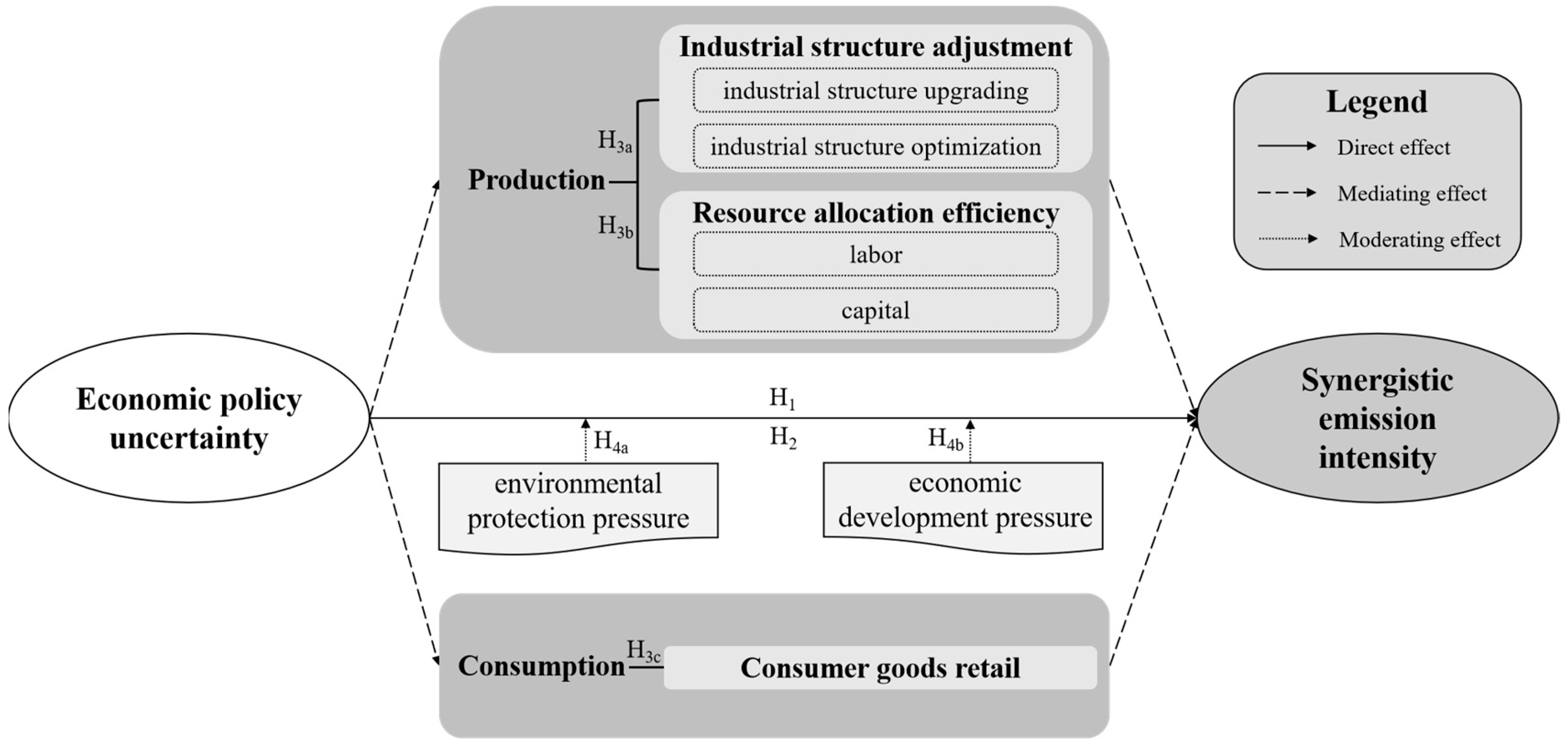
Based on the above analysis, here, a theoretical framework (Figure 1) of the impact of EPU on SEI was constructed.

2.2. The Empirical Model

While the traditional panel estimation method overlooks the potential spatial correlations, Anselin [51] incorporated the often-neglected spatial factor into the measurement model. This integration ensures that the estimated results are more accurate and closely aligned with reality. If the spatial autocorrelation test yields significant results, a spatial econometric model can be further constructed to explore the magnitude and direction of EPU spillover. This paper opted for the spatial Durbin model (SDM) to examine the spatial spillover effects of EPU and its associated influencing factors.
The specific model is as follows:
l n S E I i t = α 0 + ρ W i t l n S E I i t + α 1 E P U i t + θ 1 W i t E P U i t + α X X i t + θ X W i t X i t + σ i + μ t + ε i t
In Equation (1), the subscripts i and t represent the variables of the i-th city in the t-th year. SEIit denotes the synergistic emission intensity of air pollutants and CO2. lnSEIit is its logarithm, and EPUit is economic policy uncertainty. Xit is a vector composed of a set of control variables, including the level of infrastructure construction (empit), foreign direct investment (FDIit), the number of industrial enterprises above the scale (nieit), and the investment for controlling pollutant gases (ewgtit). Wit stands for the spatial weight matrix. WitlnSEIit represents the spatial lag of the SEIit in this city, WitEPUit is the spatial lag of EPUit, and WitXit represents the spatial impact of the adjacent regional explanatory variable on the regional explained variable. α0 is a constant term, while α1 and αX denote the effects of EPU and control variables on the SEI, respectively. ρ, θ1, and θX are the coefficients of the spatial lag term, used to examine the direction and degree of spatial spillover effects of SEI, EPU, and control variables. σi is the city fixed effect, μt is the year fixed effect, and εit stands for the random disturbance term. The standard errors are clustered at the city level.

2.3. Spatial Correlation Analysis

2.3.1. Spatial Weight Matrix Setting

To express the spatial correlation among regions, a geographical distance matrix, an adjacent space weight matrix, an economic distance matrix, and an economic geographic distance matrix were constructed. Specifically, the geographical distance matrix (W1) was employed to denote the spatial weight, which is the reciprocal of the distance between two adjacent cities [52]. If d is used to represent the distance between two cities, the calculation formula of geographical weight can be expressed as follows:
W 1 = 1 / d ,               a b 0 ,                       a = b
Furthermore, for the sake of robustness tests, an adjacent space matrix (W2) was built. When two cities are adjacent, the weight value is 1, otherwise it is 0, and the expression is as follows:
W 2 = 1 ,                           a   i s   a d j a c e n t   t o   b 0 ,             a   i s   n o t   a d j a c e n t   t o   b   o r   a = b
The economic distance matrix (W3) is the weighted average of adjacent space weight and economic weight [53]. This study introduced an economic distance spatial weight matrix based on the value of GDP per capita in each region into the model. The equation of the matrix is as follows:
W 3 = 1 / G D P a G D P b ,                 a b 0 ,                                                                             a = b
In Equation (4), GDPa and GDPb are the GDP of cities a and b, respectively.
According to Wan et al. [54], the economic geographic matrix (W4) can be expressed as follows:
W 4 = G D P a × G D P b / d 2 ,             a b 0 ,                                                                         a = b
In Equation (5), d 2 is the square number of the distance of cities a and b.

2.3.2. Exploratory Spatial Data Analysis

To ascertain the suitability of the spatial econometric model for this study, the Moran’s I index was utilized to investigate the spatial autocorrelation of the dependent and primary independent variables. Spatial autocorrelation pertains to regions with similar locations and variable values. In spatial econometrics, it is typically measured via Moran’s I index (I).
The calculation equation is as follows:
I = i = 1 n j = 1 n w i j [ y i E ( y i ) ] [ y j E ( y i ) ] / s 2 i = 1 n j = 1 n w i j
where s 2 = 1 n i = 1 n ( y i E ( y ) ) 2 , E ( y i ) = 1 n i = 1 n y i . n is the number of sample cities, and in this paper, n = 282. w i j stands for the spatial weight matrix. This paper mainly used a geographical distance matrix. The value range of Moran’s I is [−1, 1]. When Moran’s I > 0, it represents a positive spatial correlation; the larger the value is, the more obvious the spatial correlation is. Moran’s I < 0 indicates negative spatial correlation. The smaller the value is, the greater the spatial difference is. Moran’s I = 0 indicates spatial randomness.
Moreover, the aggregation characteristics of SEI and EPU were examined across cities in 2003, 2010, and 2017, respectively. This was carried out in order to delve deeper into the local autocorrelation patterns of urban SEI and EPU.

3. Datasets

3.1. Dependent Variable

In order to quantitatively reflect the overall emission intensity of CO2 and air pollutants, following Mao et al. [55], this paper applied the SEI indicator as a quantitative measuring scale. Different pollutants are converted into one “abstract pollutant” by assigning them appropriate weight factors. This approach has been used in numerous analyses [56,57]. To formulate the SEI indicator, the CO2 and air pollutants are converted and “integrated” through a linear formula, as follows:
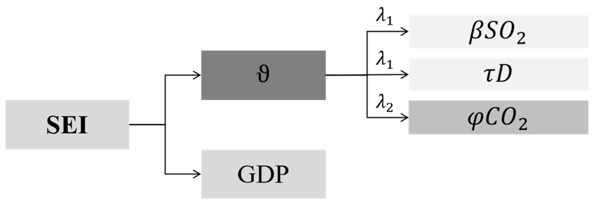
S E I = ϑ / G D P = [ λ 1 × ( β S O 2 + τ D ) + λ 2 × φ C O 2 ] / G D P
where ϑ is the combined emission equivalent of SO2, smoke and dust (D), and CO2. GDP is the average annual gross domestic product of each city. λ1 and λ2 are the relative weight factors of air pollutant emissions and greenhouse gases, respectively, used to reveal the relative importance of the two in terms of monetary value or price. β and τ denote the conversion coefficients for SO2 and smoke and dust, respectively, and φ is the conversion coefficient of CO2. As CO2 was the only greenhouse gas considered in this study, the value of φ is 1. The calculation process of SEI is shown in Figure 2.
Due to the lack of data on environmental protection tax amounts in various cities, the conversion coefficients between SO2 and smoke and dust, β and τ , were determined by referring to the tax items and tax amount tables in the environmental protection tax of various provinces in China. The average price of CO2 from 2003 to 2017 was CNY 22 (tCO2 equivalent)−1.

3.2. Measurement of Cities’ EPU in China

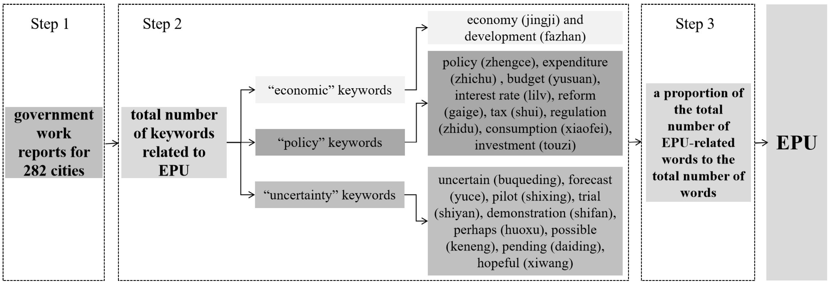
Referencing Yu et al. [58], city-level EPU indicators in China were constructed. Initially, government work reports for 282 cities were manually compiled using various information sources, including each city’s Statistical Yearbook, government websites, and local media. These city government work reports are significant official documents that reflect the work plan, particular objectives, and local government priorities for the upcoming year. They also guide lower government levels in establishing and strictly enforcing policy objectives. The reports include the targeted GDP growth rate and the policy goals of the local government, which are significant determinants of producer and consumer decisions. Secondly, the authors searched for the total number of keywords related to EPU, which can be categorized into three groups, namely, “economic” keywords, including economy (jingji) and development (fazhan); “policy” keywords, including policy (zhengce), expenditure (zhichu), budget (yusuan), interest rate (lilv), reform (gaige), tax (shui), regulation (zhidu), consumption (xiaofei), and investment (touzi); “uncertainty” keywords, containing uncertain (buqueding), forecast (yuce), pilot (shixing), trial (shiyan), demonstration (shifan), perhaps (huoxu), possible (keneng), pending (daiding), and hopeful (xiwang). The authors then summed up all occurrences of EPU-related keywords. Lastly, the EPU indicator for each city was calculated as the proportion of the total number of EPU-related words to the total number of words in that year’s government work report. The calculation process of EPU is shown in Figure 3.
The EPU indicator developed in this paper offers the following advantages. Firstly, this paper’s EPU is city-specific, enabling the investigation of city heterogeneity. Most existing studies have constructed EPU indicators based on the national or provincial level. For example, Baker et al. [59] treated China as a homogeneous entity, while Yu et al. [58] constructed EPU indicators based on provinces. Cities play a crucial role in the global emission reduction efforts, but most governments confront difficulties in lessening the effect of EPU on the co-control of CO2 and air pollution. Therefore, the design of an urban EPU indicator is more suited to the requirement for policy adjustment. Secondly, the methodology used to generate the urban EPU index in this study is more pertinent to pollutant emission behavior. Most of the existing literature conducted analyses based on the construction of EPU indexes from sources such as the South China Morning Post, an English-language newspaper in Hong Kong, China [59], or newspapers published in Mainland China [40]. In contrast, this paper used urban government work reports as the information source. These reports are officially released by the government, ensuring high authority and accuracy of their content, whereas newspaper reports may be influenced by the subjective judgment of editors or reporters. Furthermore, government work reports often outline the main policies and plans for the upcoming year, serving as a valuable information source for Chinese market players and significantly impacting the choices made by consumers and producers.

3.3. Channel Variables

In this paper, whether the production side is a potential mechanism for EPU to influence SEI is explored in two aspects: industrial structure adjustment and resource allocation efficiency. Industrial structure adjustment can be bifurcated into industrial structure upgrading and industrial structure rationalization, and the industrial-structure-level coefficient was chosen to measure the degree of industrial structure upgrading [60]. The following equation: I S U i t = ω = 1 3 ω × ς i t ω , where i denotes the city, t denotes the time, and ω denotes the industry, indicates the ratio of the value added of the industry to the gross domestic product of the region. The rationalization of industrial structure is usually measured by the Euclidean distance (ED), and the larger the ED is, the more irrational the industrial structure will be. Assuming that a country has multiple economic sectors (with a total number of k), ED between the proportion of industrial value added and the proportion of labor force employment is defined by the following equation: E D i = L F E i / k L F E k V A i / k V A k ,   E D = i E D i 2 , where LFEi and VAi are used to represent the labor force employment and industrial value added of sector i, respectively. EDi is the distance between the labor force employment share of sub-sector i and the industry value added share, and ED is the squared sum of the distance between the labor force share of all sub-sectors and the industry value added share, which represents the Euclidean distance between the overall labor force employment share and the industry value added share. In this paper, the three industrial sectors were selected, so k = 3 and 0 ≤ ED 3 . The larger the ED, the more distorted the industrial structure, i.e., the more irrational the industrial structure.
This paper used the allocation efficiency of two elements, labor (DL) and capital (DK), to measure the allocation efficiency of production factors, both of which are calculated as shown in the following equations: D L t = M P L t / χ t = ξ t Y t / L I t χ t , and D K t = M P K t / γ t = η t Y t / K I t γ t . Here, Yt represents output, LIt represents labor input, expressed as the number of employed persons at the end of the year, KIt represents capital input, expressed as the capital stock, while ξ t and η t represent the output elasticity coefficients of labor and capital, respectively. Using the traditional least squares method to estimate the output elasticity coefficients of labor and capital at the city level, the results showed that at the city level, the estimated output elasticity coefficients for labor and capital were 0.125 and 0.712, respectively, representing the wage of labor and the interest rate of capital, respectively. The wage of labor was expressed as wage income from disposable income per capita and was adjusted to the 2003 price level using the GDP deflator. The interest rate was expressed using the average of the legal loan tenor rates of financial institutions. Larger values of DL and DK represent more distorted allocation of labor and capital, i.e., less efficient allocation.
In exploring whether the consumption side could be a potential channel for EPU to influence SEI, the growth rate of total urban retail sales of social consumer goods was selected as the consumption-side indicator. Among various types of consumption-related statistics, the total urban retail sales of social consumer goods offered the most direct data expressing China’s consumption demand. Total urban retail sales of social consumer goods are the total amount of consumer goods sold directly to urban and rural residents, as well as social groups, by various industries of the national economy. It is an important indicator for analyzing the changes in China’s retail market and reflecting the degree of economic prosperity.

3.4. Control Variables

The following control variables were chosen in order to investigate the spatial effects of EPU on SEI in light of the fact that elements such as environmental infrastructure development, openness, urban economy, and the degree of emphasis on waste gas treatment have significant effects on the reduction of air pollution and carbon emissions. (1) The scales of the personnel in environmental protection agencies were used to characterize the level of environmental infrastructure development (eicit) because environmental protection administrative agencies and personnel scales could reflect the division of government environmental rights. This enables local governments to exert their information advantages and coordinate the allocation of funds and personnel in the process of environmental governance [48], thereby enhancing the Green Total Factor Energy Efficiency of local enterprises and implementing environmental protection [61]. (2) Openness was measured by foreign direct investment (FDIit). Foreign direct investment is often considered highly correlated with pollutant emissions [62], because heavy-polluting and high-energy-consuming industries are among those that receive investment, and the increasing production will promote carbon dioxide emissions. As a result, regional environmental pollution may be exacerbated and have a negative impact on regional green development [63]. (3) The urban economy was expressed as the number of industrial enterprises above the designated size (nieit) [64]. As key components of the industrial chain, these enterprises are the core of the organizational structure. The larger the size of the enterprise, the higher the productivity, and the more efficient the rate of industrial agglomeration, thus helping to attract more small and medium-sized enterprises and promoting the development of the entire urban economy [65]. The more industrial enterprises above the designated size, the higher the degree of urban economic development. However, as a major source of air pollution, the number of industrial enterprises above the designated size is closely linked to the possibility of urban air pollution. (4) The degree of emphasis on waste gas treatment (ewgtit) was characterized by utilizing the operating costs of waste gas treatment facilities. Studies have shown that the government’s fiscal expenditure on environmental protection has a significant effect on the improvement of environmental quality, which is the most effective and direct expenditure of local governments in environmental governance in China [66]. Due to the different levels of economic development of different cities, under the premise of limited budgets, cities’ governments need to strike a balance between fiscal expenditure and environmental pollution. Therefore, the allocation of funds and the operational input of waste gas treatment projects can represent the local government’s emphasis on waste gas treatment projects [67].

3.5. Data Sources

The sample data in this paper are panel data of 282 cities in China from 2003 to 2017 (Tibet, Hong Kong, Macao, and Taiwan Province of China were excluded from the study due to a lack of data). CO2 emissions data were from the University of Colorado Cooperative Institute for Environmental Sciences, USA (CIRES). GDP and FDI were calculated at constant prices in 2003. The China Statistical Yearbook for Regional Economy, China City Statistical Yearbook, China Statistical Yearbook, and China Statistical Yearbook on Environment are where the original data came from. Table 1 shows the description and statistics of the relevant variables (missing values were filled in via interpolation and means).

4. Results and Discussion

4.1. Basic Statistical Analysis

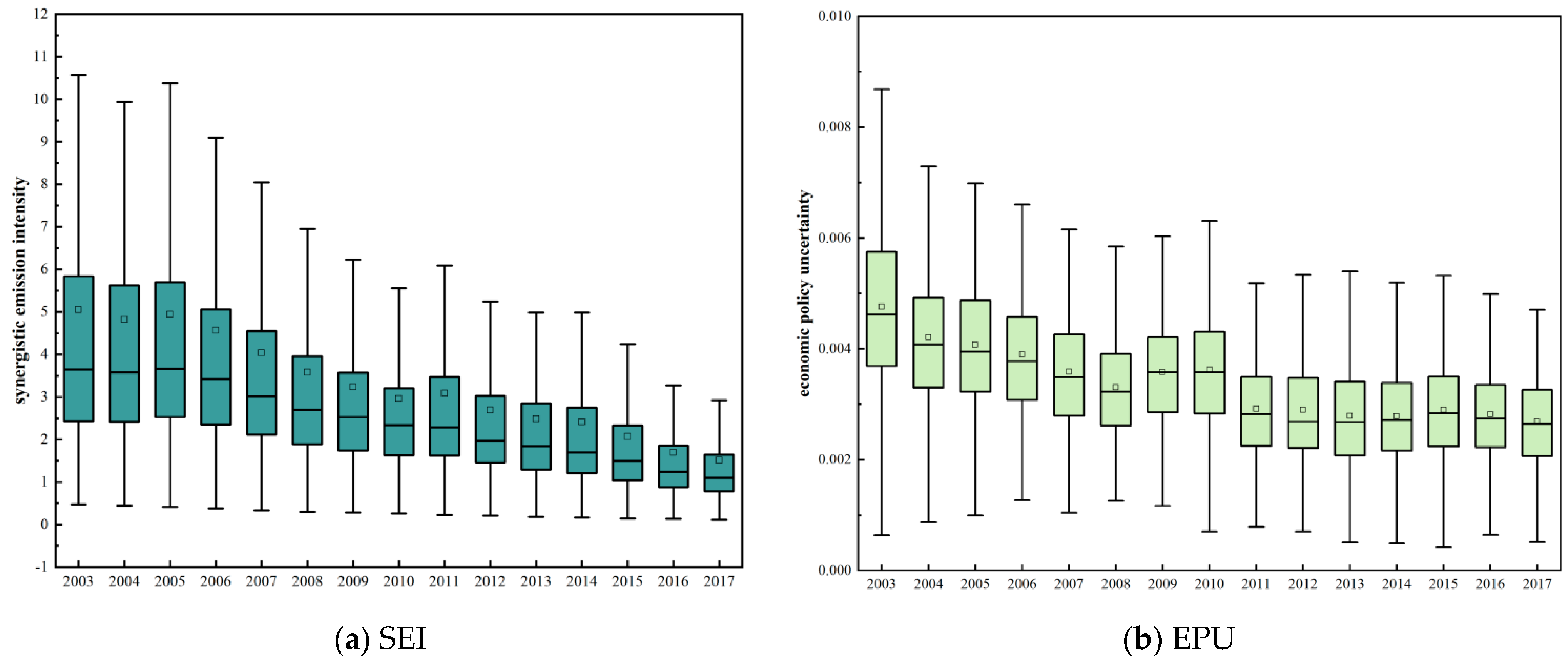
Before carrying out the econometric analysis, it was necessary to establish a basic statistical identification of China’s SEI and EPU. Figure 4 depicts the temporal evolution of SEI and EPU. From 2003 to 2017, both SEI and EPU generally exhibited a declining trend. SEI reached its peak in 2003, after which it steadily decreased. The average level of EPU in China’s cities decreased from 0.0047 in 2003 to 0.0027 in 2017, a reduction of 43.552%. This implies a gradual improvement in the stability of economic policies.
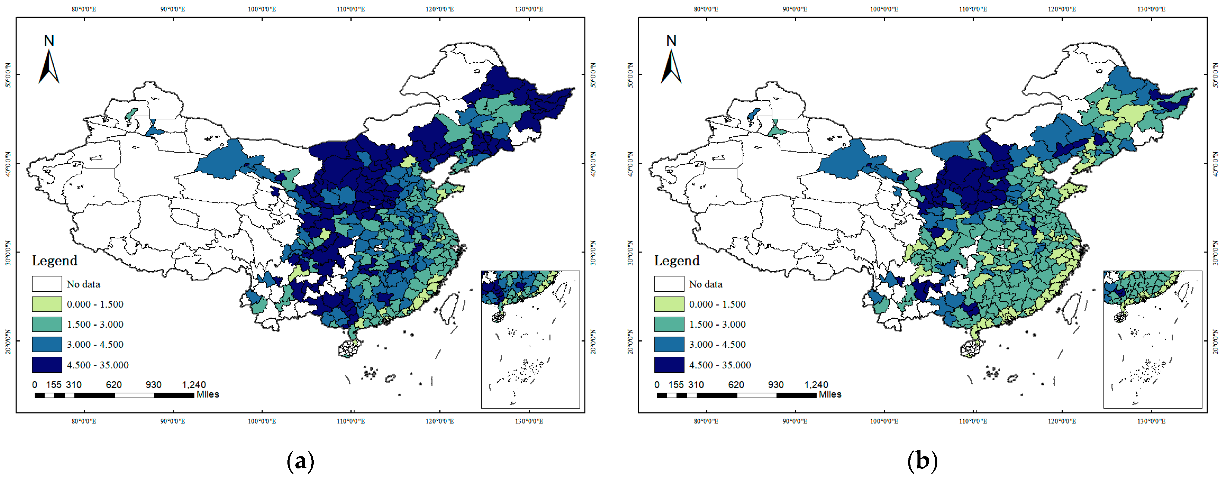
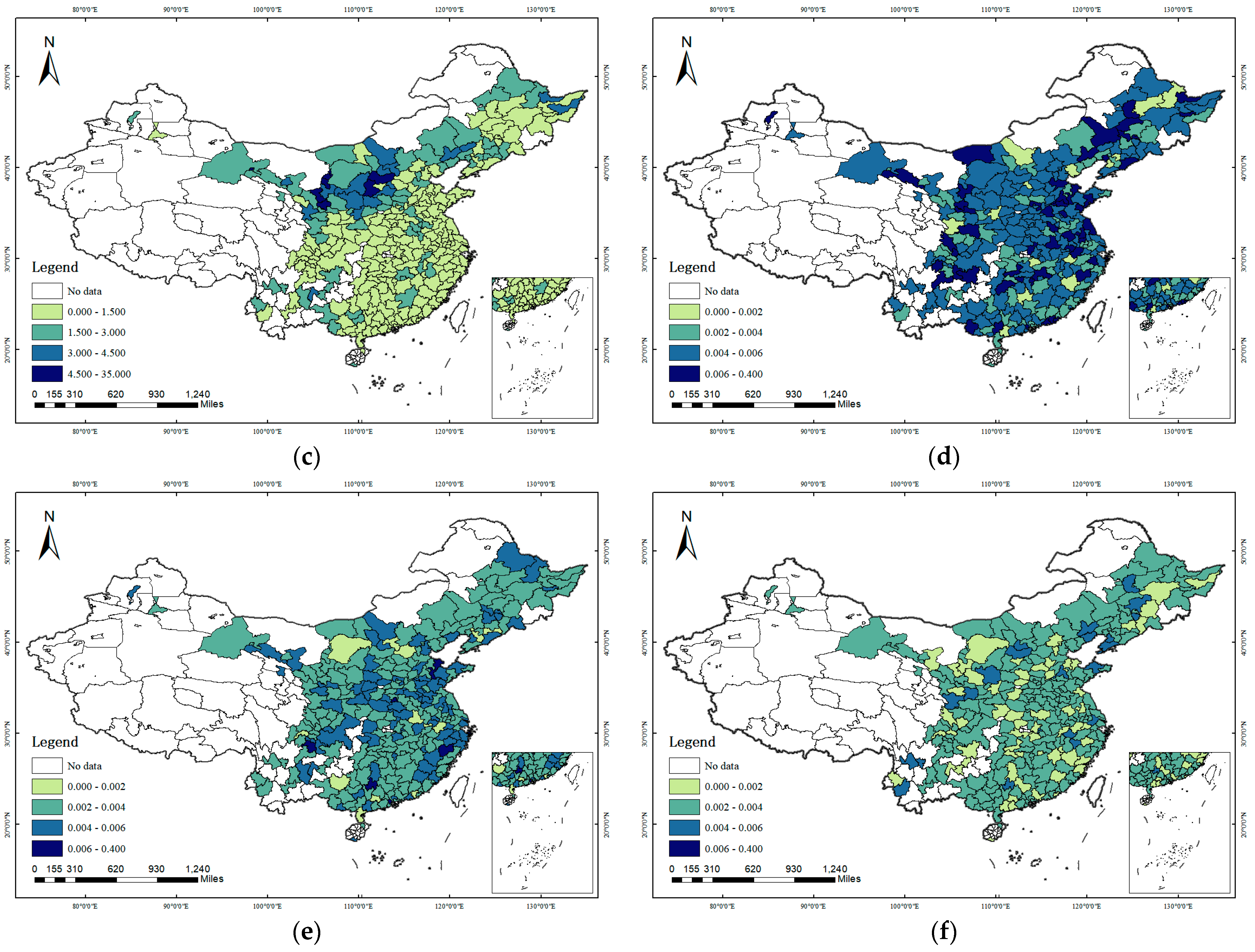
Additionally, the annual average spatial distributions of SEI and EPU were observed. As evident from Figure 5, the spatial distributions of SEI and EPU exhibited significant regional disparities. A distinct spatial club phenomenon was observed for SEI, leading to the formation of a pollution zone in the Beijing–Tianjin–Hebei region (the Beijing–Tianjin–Hebei region includes Beijing, Tianjin, Shijiazhuang, Tangshan, Qinhuangdao, Handan, Xingtai, Baoding, Zhangjiakou, Chengde, Cangzhou, Langfang, and Hengshui) and the Fenwei Plain (the Fenwei Plain includes Xi’an, Baoji, Xianyang, Weinan, and Tongchuan in Shaanxi Province, Taiyuan, Jinzhong, Lvliang, Linfen, and Yuncheng in Shanxi Province, and Luoyang and Sanmenxia in Henan Province, etc.). As for EPU, it consistently registered higher values in the northeast region (including Dandong, Dalian, Panjin, Baishan, Hegang, Qitaihe, etc.) and the Shandong Peninsula (including Zibo, Qingdao, Weifang, Rizhao, Dongying, etc.).

4.2. Empirical Analysis

4.2.1. Spatial Correlation Test

The regional Moran’s I test, as depicted in Equation (6), was employed to compute the Moran’s I index, the statistical Z-value under the geographical distance matrix of the SEI and EPU in China. The specific calculation results are shown in Table 2. The results revealed that the majority of Moran’s I indexes of SEI and EPU were significantly positive, indicating spatial correlations among the aforementioned variables. It is noteworthy that the Moran’s I indexes of EPU were negative in 2003 and 2004. This finding suggests that the spatial distribution of EPU in Chinese cities during the early period exhibited a certain degree of dispersion. Specifically, cities with similar levels of EPU tended to be located at spatially distant locations rather than adjacent ones. This negative correlation in the spatial distribution of EPU implies greater dissimilarity in EPU characteristics among neighboring cities. This phenomenon may be attributed to the comprehensive economic system reforms undertaken in China in 2003, along with the gradual promotion of governmental institutional reforms. These reforms mandated the coordination of “decision-making, execution, and supervision” among governmental departments. While some regions had already completed their governmental institutional reforms by 2003, most regions were still in the process of fact-finding and preparation. Consequently, there emerged a spatial dispersion of economic policy uncertainty.
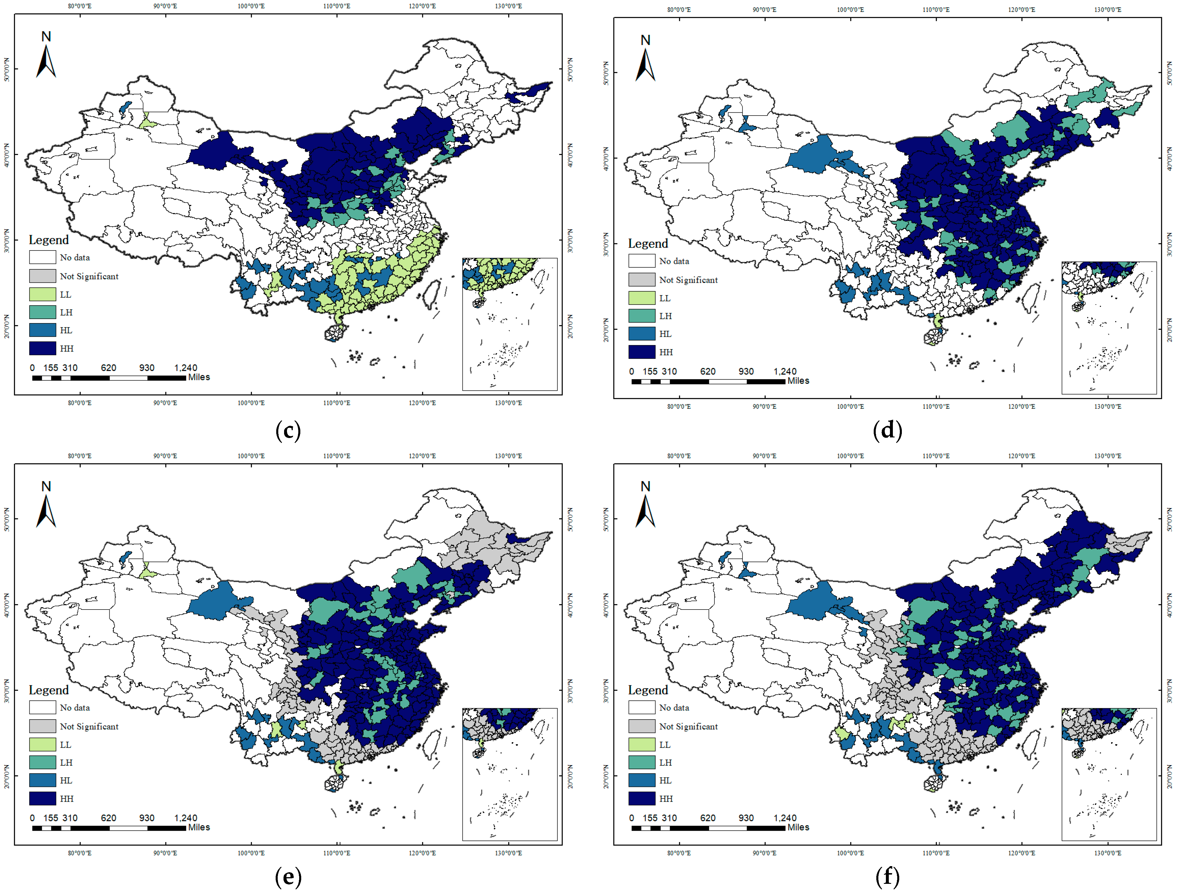
For a more detailed study of local autocorrelation patterns, LISA maps are presented in Figure 6. The figure reveals that the North China Plain, the Beijing–Tianjin–Hebei region, and the Fenwei Plain were the main distribution areas for the HH agglomeration (high–high agglomeration: high-SEI areas surrounded by high-SEI areas) of SEI under the geographic distance matrix. Additionally, the LL agglomeration (low–low agglomeration: low-SEI regions surrounded by low-SEI regions) of SEI was primarily observed in cities in southeast China, while the number of cities with HL agglomeration (high–low agglomeration: high-SEI regions surrounded by low-SEI regions) and LH agglomeration (low–high agglomeration: low-SEI regions surrounded by high-SEI regions) of SEI was relatively small. In the case of EPU, the HH agglomeration was primarily distributed in the northeastern area, central China, and southeast China, while the number of cities with LL, HL, and LH agglomeration was comparatively low. Considering these observations, it was imperative to employ a spatial econometric model for quantitative empirical research, as SEI and EPU in China exhibited considerable spatial correlation features.

4.2.2. Test Results of the Model Selection

As shown in Table 3, the results of the Hausman test indicated the necessity of a fixed-effects model. The results of the LR test advocated for the use of a two-way fixed-effects model. The LR test results also demonstrated that a spatial Durbin, two-way fixed-effects model should be used.

4.2.3. Empirical Results of the Spatial Durbin Model

In this paper, the impact of the EPU on SEI and its spatial spillover effect was estimated based on Equation (1), with the results presented in Table 4. Columns (1) and (3) display the impact and spillover effects of EPU on SEI without considering any control variables, while columns (2) and (4) show the spillover impact when city-level control variables were factored in. The findings in columns (1) and (2) reveal that the coefficients of EPU were significantly positive, irrespective of the inclusion of control variables in the regression model. When EPU increases by one unit, the SEI will increase by 586.5% (p < 0.05) and 675.6% (p < 0.01), respectively. This suggests that an increase in EPU corresponds to a rise in the intensity of air pollution and carbon emissions, thereby supporting Hypothesis H1. The results in columns (3) and (4) show that the coefficients of EPU were 152.865 and 144.606, which are both statistically significantly positive at the 1% level of significance, affirming H2 that EPU exerts a significant spatial spillover effect on the SEI.
To thoroughly examine the impact of EPU on SEI, the spatial effect decomposition approach of the spatial econometric model was used to split the total effect into direct and indirect effects. The indirect effect, also known as the spatial spillover effect, was utilized to analyze the influence of the EPU on the SEI in nearby cities. Conversely, the direct effect was used to examine the impact of EPU on the local SEI. Table 5 presents the effect decomposition derived from the estimations based on Equation (1) in Table 4. As can be observed, when EPU increases by one unit, the intensity of synergistic emissions of air pollutants and CO2 of local cities, adjacent cities, and total cities will surge by 930.9% (p < 0.01), 69162.7% (p < 0.01), and 70093.6% (p < 0.01), respectively. The direct effect suggested that EPU is a substantial contributor to the rise in local SEI. This finding is in line with previous estimations. When the geographical distance matrix was used as the spatial weight, the indirect effect results showed that the EPU had a significant positive spatial spillover effect on the SEI. Additionally, a comparison of the coefficients indicated that the spatial spillover effect of EPU on the SEI was greater than the direct effect. This suggests that reducing local EPU alone is not sufficient to decrease SEI. Instead, reducing EPU spillovers from neighboring cities and actively taking part in the inter-regional cooperation for reducing EPU are key for pursuing the synergistic reduction in air pollution and carbon emissions.

4.3. Robustness Check

This paper adopted two methods to test the robustness of the benchmark regression results: replacing the spatial weight matrix and altering the dependent variable. Based on Equation (1), Table 6 shows the estimation results of replacing the W1 with the W2, W3, and W4, respectively. As for total effects, under the three spatial matrices, W2, W3, and W4, when the EPU increases by one unit, the SEI of total cities will significantly increase by 4526.4% (p < 0.01), 1504.6% (p < 0.05), and 2867.1% (p < 0.01), respectively. The findings demonstrated the robustness of the benchmark regression, showing that the increase in EPU raised the SEI of both local and surrounding cities. Moreover, the findings also demonstrated that the positive spatial spillover impact of EPU on SEI was not confined to geographically proximate cities, but also extended to economically adjacent cities.
Table 7 displays the estimation results of substituting the dependent variable to measure the emission intensity of carbon and SO2 separately based on Equation (1). Under the geographical distance matrix, the coefficients of the direct, indirect, and total effects of EPU were all significantly positive. As for total effects, the results in columns (5) and (6) show that the coefficients of EPU were 320.750 and 1338.137, which were both statistically significantly positive. This suggests that EPU can significantly increase not only the local carbon and SO2 emission intensities but also those of nearby cities via spatial spillover effects. This finding is consistent with the baseline results of this study, as shown in Table 5.

4.4. Channel Analysis

In this section, this paper aims to explore the potential channels through which EPU affects SEI, thereby testing H3a, H3b, and H3c. The results, displayed in columns (1) and (2) of Table 8, showed that when EPU increases by one unit, the ISU of total cities will decrease by 21375.7% (p < 0.1), while the ED will increase by 23805.4% (p < 0.05). These results, based on Equation (1), indicate that EPU can impact SEI by influencing production-side factors, such as inhibiting industrial structure upgrading and increasing industrial structure distortion, thereby validating H3a. To attract investment for economic development, some local governments tend to externally intervene in the prices of production factors, i.e., they depress these prices. Consequently, enterprises may be more inclined to use low-cost tangible factors, which leads to a dependency on resource-intensive industries for local economic development. This also makes it profitable for those outdated production capacities that need to be eliminated to persist, thereby limiting the upgrading of the industrial structure [68]. This lock-in effect of the traditional industrial structure and sloppy economic growth has been an important cause of China’s environmental pollution problems in recent years [69].
Furthermore, the results represented in columns (3) and (4) based on Equation (1) indicate that when EPU increases by one unit, the DL of total cities will increase by 63,689.7% (p < 0.05). Distortions in the labor market serve as one of the mechanisms through which EPU influences the SEI. This may be attributed to the combined effect of the “promotion tournament” and fiscal decentralization. Under these circumstances, local governments may reduce labor wages to enhance investment attractiveness, thereby decreasing enterprise costs and attracting foreign investment in the short term. However, lower wages can constrain the upgrading of workers’ skills, indirectly impeding the potential for labor transfer to higher-level industries and exacerbating the mismatch of labor resources. This situation may lead enterprises to increase the input of tangible resources to improve business performance, subsequently reducing the initiative of independent innovation. It is also not conducive to the adoption of cleaner production technologies, the development of pollution control equipment, and the reduction in energy consumption per unit of output, thereby aggravating environmental pollution [70].
The results shown in columns (4) and (5) based on Equation (1) indicate that the total effects of EPU on capital allocation efficiency (26.065) and the growth rate of total retail sales of consumer goods (100.03) were not significant. This indicates that neither capital allocation efficiency nor the consumption side are underlying channels for EPU’s influence on the SEI. Therefore, H3b is partially supported, while H3c is not valid.

4.5. Heterogeneity Analysis

4.5.1. Environmental Protection Pressure

In 2002, the Former Ministry of Environmental Protection identified 113 cities as key environmental protection cities [71], requiring urgent air pollution prevention and control measures. The national 11th Five-Year Plan for environmental protection further stated that these 113 cities were of higher priority for air pollution control. Additionally, more sophisticated and comprehensive emission-monitoring systems have been set up for these cities, which results in key environmental protection cities having greater pressure to protect the environment compared to non-key environmental protection cities. Therefore, this paper divided the entire sample into two groups: key environmental protection cities (KEP; the cities with higher environmental protection pressure, including 112 cities (the city of Lhasa was not included in this paper because of a serious lack of data)) and non-key environmental protection cities (NKEP; the cities with lower environmental protection pressure, including 170 cities). The regression results are shown in Table 9.
According to the results in columns (5) and (6), the coefficients of EPU in NKEP and KEP cities, calculated via Equation (1), were 417.935 (p < 0.05) and −70.932 (p < 0.01), respectively. Upon considering the impact of environmental protection pressure, it was discovered that EPU in NKEP cities had a stronger inhibitory effect on the co-control of air pollutants and CO2 than in KEP cities. This suggests that pressure from the central government for environmental protection is indeed an important mechanism for curtailing the economic incentives of local governments and promoting their attention to environmental management and pollution reduction. This finding validates hypothesis H4a, which posits that environmental protection pressure is a significant mechanism for curbing the growth of air pollution and carbon emissions.

4.5.2. Economic Development Pressure

Under increased economic development pressure, local governments often resort to extensive economic development methods. They mobilize various resources and gradually relax their pollution monitoring and environmental enforcement of high-polluting enterprises to boost local GDP and secure promotional advantages [72]. Therefore, in order to explore the varying effect of EPU on the SEI under different economic development pressures, the authors followed the method of Zhao et al. [73] and measured the economic development pressure of local governments using the ranking of the GDP growth rate of each city in the previous year within its respective province (eco_rank). A lower GDP growth rate ranking for a city in the previous year implies higher GDP growth pressure in the current year. The regression results are shown in Table 10.
As can be seen from the findings based on Equation (1) in Table 10, the direct effect of the interaction term between GDP growth rate ranking and EPU was significantly negative (p < 0.05), while the indirect and total effects were not significant. When the interaction term between GDP growth rate ranking and EPU decreases by one unit, the SEI of local cities, adjacent cities, and total cities will decrease by 977.7% (p < 0.05) and increase by 6669.3% (p > 0.10) and 5691.6% (p > 0.10), respectively. This indicates that a city with a lower GDP growth rate ranking in the province in the previous year faces more economic development pressure in the current year, which in turn amplifies the impact of EPU on increasing pollutant emissions. This finding is consistent with H4b. This is likely because the pressure from economic growth significantly influences governmental operations. Governments typically embrace short-term development strategies that provide immediate economic advantages when they are under intense pressure for economic growth [74]. Unavoidably, this will result in distortions in resource investment and the allocation of production elements.

5. Conclusions and Implications

The authors constructed a new city-level EPU measurement method and employed a spatial Durbin, two-way fixed effects model to investigate the impact of EPU on the SEI across 282 cities in China. Moreover, the channels through which EPU affects the SEI were proposed and empirically tested and heterogeneity analysis was conducted to delve deeper into the influence of government environmental protection and economic development pressure on the relationship between EPU and SEI. The findings indicated the following: (1) Both the SEI and EPU exhibited a declining trend. The SEI steadily decreased and EPU decreased from 0.0047 in 2003 to 0.0027 in 2017, a reduction of 43.552%. The SEI and EPU in China exhibited positive spatial correlation features. A distinct spatial club phenomenon was observed for SEI in the Beijing–Tianjin–Hebei region and the Fenwei Plain. EPU consistently registered higher values in the northeast region and the Shandong Peninsula. (2) EPU imposed a significantly positive impact on the SEI in adjacent cities via the spatial spillover effect. When EPU increases by one unit, the intensity of synergistic emissions of air pollutants and CO2 of local cities, adjacent cities, and total cities will surge by 930.9%, 69,162.7%, and 70,093.6%, respectively. (3) The channel analysis suggested that EPU generally affects the SEI through two channels: industrial structure and allocative efficiency. Specifically, when EPU increases by one unit, the level of industrial structure upgrading will decrease by 21,375.7%, while industrial structure distortion and labor market distortion will increase by 23,805.4% and 63,689.7%, respectively. (4) The effect of EPU on the SEI can be diminished by increased environmental pressure but is enhanced by increased economic development pressure. It was found that EPU in NKEP cities had a stronger inhibitory effect on the co-control of air pollutants and CO2 than KEP cities, while the pressure of a city’s economic development ultimately magnified the impact of EPU on increasing pollutant emissions.
Regarding these empirical findings, this paper puts forth several policy suggestions for the government’s consideration. The hope is that this paper can contribute to more effective and sustainable economic and environmental policies. Firstly, it is recommended that policymakers ensure the continuity and stability of domestic economic policies. This is to mitigate the adverse effects of economic policy changes on cities’ synergistic control of air pollutants and CO2 emissions.
Secondly, considering the strong spatial correlation between the SEI and EPU, it is crucial for the central government to consider the design of a joint pollution control system and bolster inter-regional environmental governance cooperation. Moreover, the vertical pressure exerted by the central government on environmental protection serves as a crucial mechanism. This mechanism curbs the financial incentives of local governments, compelling them to concentrate on environmental management and reduce pollution emissions. Meanwhile, cities should proactively reduce local EPU and concurrently monitor the EPU of other cities. By taking timely and effective measures, cities can prevent the adverse impacts of economic uncertainty from adjacent cities on themselves. Furthermore, to deter local governments from engaging in “free-riding” and a “race to the bottom”, it is imperative for the cities to fortify the public environmental monitoring system and implement a sound environmental management policy.
Thirdly, it is essential to further promote the enhancement of the industrial structure, eliminate distortions within this structure, and improve labor market construction to improve the efficiency of labor resource allocation. To achieve industrial structure upgrading and transform the economic development mode, the strict regulation of polluting industries is necessary. Promoting the optimal allocation of factors and strengthening environmental supervision, as well as monitoring, could be helpful. Additionally, cities should keep promoting the free movement of labor resources and other production factors between cities. This involves removing barriers to industrial development across different cities and implementing corresponding policies related to household registration, education, healthcare, pensions, and other social aspects. The creation of commuter networks between cities with varying levels of productivity can enhance the effectiveness of resource distribution.
Author Contributions

Conceptualization, X.Y., G.C. and F.L.; methodology, X.Y., C.Q. and Y.W.; software, X.Y.; validation, X.Y. and L.S.; formal analysis, X.Y., G.C., C.Q., Z.C. and Y.W.; investigation, F.L.; resources, C.Q. and L.S.; data curation, Z.C.; writing—original draft, X.Y., G.C., Z.C. and Y.W.; writing—review and editing, G.C., C.Q., L.S. and F.L.; visualization, L.S.; supervision, G.C. and L.S.; project administration, L.S.; funding acquisition, X.Y. and L.S. All authors have read and agreed to the published version of the manuscript.

Funding

This research was funded by the Outstanding Innovative Talents Cultivation Funded Programs 2023 of Renmin University of China and the National Key R&D Program of China (No. 2018YFC0213702) funded by Ministry of Science and Technology of the People’s Republic of China.

Data Availability Statement

The original contributions presented in the study are included in the article, further inquiries can be directed to the corresponding author.

Conflicts of Interest

The authors declare no conflict of interest.

References

  1. Al-Thaqeb, S.A.; Algharabali, B.G. Economic policy uncertainty: A literature review. J. Econ. Asymmetries 2019, 20, e00133. [Google Scholar] [CrossRef]
  2. Gu, K.; Dong, F.; Sun, H.; Zhou, Y. How economic policy uncertainty processes impact on inclusive green growth in emerging industrialized countries: A case study of China. J. Clean. Prod. 2021, 322, 128963. [Google Scholar] [CrossRef]
  3. Zheng, J.; Mi, Z.; Coffman, D.; Milcheva, S.; Shan, Y.; Guan, D.; Wang, S. Regional development and carbon emissions in China. Energy Econ. 2019, 81, 25–36. [Google Scholar] [CrossRef]
  4. Ministry of Ecology and Environment and Other Seven Departments. Implementation Plan for Synergy of Pollution Reduction and Carbon Reduction. 2022. Available online: https://www.gov.cn/zhengce/zhengceku/2022-06/17/content_5696364.htm (accessed on 6 March 2023).
  5. Xiao, H.; Zhou, Y.; Zhang, N.; Wang, D.; Shan, Y.; Ren, J. CO2 emission reduction potential in China from combined effects of structural adjustment of economy and efficiency improvement. Resour. Conserv. Recycl. 2021, 174, 105760. [Google Scholar] [CrossRef]
  6. Anwar, M.N.; Shabbir, M.; Tahir, E.; Iftikhar, M.; Saif, H.; Tahir, A.; Murtaza, M.A.; Khokhar, M.F.; Rehan, M.; Aghbashlo, M.; et al. Emerging challenges of air pollution and particulate matter in China, India, and Pakistan and mitigating solutions. J. Hazard. Mater. 2021, 416, 125851. [Google Scholar] [CrossRef] [PubMed]
  7. Yang, L.; Hong, S. Impact of the clean energy structure of building operation on the co-benefits of CO2 and air pollutant emission reductions in Chinese provinces. J. Clean. Prod. 2023, 413, 137400. [Google Scholar] [CrossRef]
  8. Wang, Y.; Wen, Y.; Zhu, Q.; Luo, J.; Yang, Z.; Su, S.; Wang, X.; Hao, L.; Tan, J.; Yin, H.; et al. Real driving energy consumption and CO2 & pollutant emission characteristics of a parallel plug-in hybrid electric vehicle under different propulsion modes. Energy 2022, 244, 123076. [Google Scholar] [CrossRef]
  9. Jiao, J.; Huang, Y.; Liao, C. Co-benefits of reducing CO2 and air pollutant emissions in the urban transport sector: A case of Guangzhou. Energy Sustain. Dev. 2020, 59, 131–143. [Google Scholar] [CrossRef]
  10. Zeng, A.; Mao, X.; Hu, T.; Xing, Y.; Gao, Y.; Zhou, J.; Qian, Y. Regional co-control plan for local air pollutants and CO2 reduction: Method and practice. J. Clean. Prod. 2017, 140, 1226–1235. [Google Scholar] [CrossRef]
  11. Lu, Z.; Huang, L.; Liu, J.; Zhou, Y.; Chen, M.; Hu, J. Carbon dioxide mitigation co-benefit analysis of energy-related measures in the air pollution prevention and control action plan in the Jing-Jin-Ji region of China. Resour. Conserv. Recycl. 2019, 1, 100006. [Google Scholar] [CrossRef]
  12. Mao, X.; Zeng, A.; Hu, T.; Xing, Y.; Zhou, J.; Liu, Z. Co-control of local air pollutants and CO2 from the Chinese coal-fired power industry. J. Clean Prod. 2014, 67, 220–227. [Google Scholar] [CrossRef]
  13. Davis, S.J. Rising Policy Uncertainty; National Bureau of Economic Research: Cambridge, MA, USA, 2019. [Google Scholar]
  14. Wang, Y.; Chen, C.; Huang, Y. Economic policy uncertainty and corporate investment: Evidence from China. Pac. Basin Financ. J. 2014, 26, 227–243. [Google Scholar] [CrossRef]
  15. Li, Z.; Su, C.; Moldovan, N.C.; Umar, M. Energy consumption within policy uncertainty: Considering the climate and economic factors. Renew. Energ. 2023, 208, 567–576. [Google Scholar] [CrossRef]
  16. Shi, X.; Yu, J.; Cheong, T.S. Convergence and distribution dynamics of energy consumption among China’s households. Energ. Policy 2020, 142, 111496. [Google Scholar] [CrossRef]
  17. Han, L.; Zhou, W.; Li, W.; Li, L. Impact of urbanization level on urban air quality: A case of fine particles (PM2.5) in Chinese cities. Environ. Pollut. 2014, 194, 163–170. [Google Scholar] [CrossRef] [PubMed]
  18. Liang, L.; Wang, Z.; Li, J. The effect of urbanization on environmental pollution in rapidly developing urban agglomerations. J. Clean Prod. 2019, 237, 117649–117665. [Google Scholar] [CrossRef]
  19. Nguyen, T. Economic policy uncertainty and bank stability: Does bank regulation and supervision matter in major European economies? J. Int. Financ. Mark. Inst. Money 2021, 74, 101387. [Google Scholar] [CrossRef]
  20. Dang, D.; Fang, H.; He, M. Economic policy uncertainty, tax quotas and corporate tax burden: Evidence from China. China Econ. Rev. 2019, 56, 101303. [Google Scholar] [CrossRef]
  21. Yang, J.; Zheng, X. Government annual report: Decision usefulness, information accessibility and policy communication efficiency—Observations from 19 Chinese cities. Policy Stud. 2022, 43, 483–501. [Google Scholar] [CrossRef]
  22. Tu, C.; Liang, Y.; Fu, Y. How does the environmental attention of local governments affect regional green development? Empirical evidence from local governments in China. Hum. Soc. Sci. Commun. 2024, 11, 371. [Google Scholar] [CrossRef]
  23. Zheng, X.; Tan, Y.; Li, D. Navigating Environmental Governance in China’s Hog Sector: Unraveling the “Race to the Bottom” Phenomenon and Spatial Dynamics. J. Knowl. Econ. 2024, 1–38. [Google Scholar] [CrossRef]
  24. Gulen, H.; Ion, M. Policy uncertainty and corporate investment. Rev. Financ. Stud. 2016, 29, 523–564. [Google Scholar] [CrossRef]
  25. Demir, E.; Ersan, O. Economic policy uncertainty and cash holdings: Evidence from BRIC countries. Emerg. Mark. Rev. 2017, 33, 189–200. [Google Scholar] [CrossRef]
  26. Shahiduzzaman, M.; Layton, A. Changes in CO2 Emissions over Business Cycle Recessions and Expansions in the United States: A Decomposition Analysis. Appl. Energ. 2015, 150, 25–35. [Google Scholar] [CrossRef]
  27. Sheldon, T.L. Asymmetric effects of the business cycle on carbon dioxide emissions. Energy Econ. 2017, 61, 289–297. [Google Scholar] [CrossRef]
  28. Long, M.A.; Lynch, M.J.; Stretesky, P.B. The great recession, the treadmill of production and ecological disorganization: Did the recession decrease toxic releases across US states, 2005–2014? Ecol. Econ. 2018, 146, 184–192. [Google Scholar] [CrossRef]
  29. Li, X.; Liu, C.; Weng, X.; Zhou, L. Target setting in tournaments: Theory and evidence from China. Econ. J. 2019, 129, 2888–2915. [Google Scholar] [CrossRef]
  30. Wu, M.; Cao, X. Greening the career incentive structure for local officials in China: Does less pollution increase the chances of promotion for Chinese local leaders? J. Environ. Econ. Manag. 2021, 107, 102440. [Google Scholar] [CrossRef]
  31. Han, L.; Kung, J.K.S. Fiscal incentives and policy choices of local governments: Evidence from China. J. Dev. Econ. 2015, 116, 89–104. [Google Scholar] [CrossRef]
  32. Qi, Y.; Zhang, L. Local environmental enforcement constrained by central–local relations in China. Environ. Policy Gov. 2014, 24, 216–232. [Google Scholar] [CrossRef]
  33. Cai, H.; Chen, Y.; Gong, Q. Polluting thy neighbor: Unintended consequences of China’s pollution reduction mandates. J. Environ. Econ. Manag. 2016, 76, 86–104. [Google Scholar] [CrossRef]
  34. Long, W.; Hu, J. Energy-saving, and Emission-reduction Plan, Environmental Assessment and Boundary Pollution. Financ. Trade Econ. 2018, 39, 126–141. (In Chinese) [Google Scholar] [CrossRef]
  35. Zhang, B.; Chen, X.; He, G. Does Central Supervision Enhance Local Environmental Enforcement? Quasi experimental Evidence from China. J. Public Econ. 2018, 164, 70–90. [Google Scholar] [CrossRef]
  36. Bai, J.; Lu, J.; Li, S. Fiscal stress, tax competition and environmental pollution. Environ. Resour. Econ. 2019, 73, 431–447. [Google Scholar] [CrossRef]
  37. Nong, H. Have cross-category spillovers of economic policy uncertainty changed during the US–China trade war? J. Asian Econ. 2021, 74, 10132. [Google Scholar] [CrossRef]
  38. Zhou, Y.; Liu, Z.; Wu, S. The global economic policy uncertainty spillover analysis: In the background of COVID-19 pandemic. Res. Int. Bus. Financ. 2022, 61, 101666. [Google Scholar] [CrossRef] [PubMed]
  39. Ma, D.; Zhang, C.; Hui, Y.; Xu, B. Economic uncertainty spillover and social networks. J. Bus. Res. 2022, 145, 454–467. [Google Scholar] [CrossRef]
  40. Huang, Y.; Luk, P. Measuring economic policy uncertainty in China. China Econ. Rev. 2020, 59, 101367. [Google Scholar] [CrossRef]
  41. Ding, L.; Xia, H.; Shi, Y.; Cheng, S. Evolution of industrial structure and its environmental effects in the Yangtze River Economic Belt from 2000 to 2015. Saf. Environ. Eng. 2020, 27, 8–16. [Google Scholar] [CrossRef]
  42. Brogaard, J.; Detzel, A. The asset pricing implications of government economic policy uncertainty. Manag. Sci. 2015, 61, 3–18. [Google Scholar] [CrossRef]
  43. Li, L.; Hong, X.; Wang, J. Evaluating the impact of clean energy consumption and factor allocation on China’s air pollution: A spatial econometric approach. Energy 2020, 195, 116842. [Google Scholar] [CrossRef]
  44. Liu, C.; Gao, J. Management by objectives and misallocation of resources of local economic growth. Commer. Res. 2020, 10, 1–9. (In Chinese) [Google Scholar] [CrossRef]
  45. Altig, D.; Baker, S.; Barrero, J.M.; Bloom, N.; Bunn, P.; Chen, S.; Davis, S.J.; Leather, J.; Meyer, B.; Mihaylov, E.; et al. Economic uncertainty before and during the COVID-19 pandemic. J. Public Econ. 2020, 191, 104274. [Google Scholar] [CrossRef] [PubMed]
  46. Sajid, M.J.; Niu, H.L.; Liang, Z.J.; Xie, J.; Rahman, M.H.U. Final consumer embedded carbon emissions and externalities: A case of Chinese consumers. Environ. Dev. 2021, 39, 100642. [Google Scholar] [CrossRef]
  47. Lin, W.; Xiao, Y.; Yu, H.; Shen, S. Does vertical environmental protection pressure promote convergence of urban air pollution? J. Innov. Knowl. 2022, 7, 100186. [Google Scholar] [CrossRef]
  48. Wu, H.; Hao, Y.; Ren, S. How do environmental regulation and environmental decentralization affect green total factor energy efficiency: Evidence from China. Energy Econ. 2020, 91, 104880. [Google Scholar] [CrossRef]
  49. Yu, Y.; Wang, Z.; Liu, D.; Fu, L. Changes in officials, total factor productivity fluctuation and government transformation: Evidence from Chinese prefecture cities. Pac. Econ. Rev. 2021, 26, 283–299. [Google Scholar] [CrossRef]
  50. Liu, D.; Xu, C.; Yu, Y.; Rong, K.; Zhang, J. Economic Growth Target, Distortion of Public Expenditure and Business Cycle in China. China Econ. Rev. 2020, 63, 101373. [Google Scholar] [CrossRef]
  51. Anselin, L. Spatial externalities, spatial multipliers and spatial econometrics. Int. Reg. Sci. Rev. 2003, 26, 153–166. [Google Scholar] [CrossRef]
  52. Vega, S.; Elhorst, J.P. The Slx model. J. Reg. Sci. 2015, 55, 339–363. [Google Scholar] [CrossRef]
  53. Shao, S.; Li, X.; Cao, J.; Yang, L. China’s economic policy choices for governing smog pollution based on spatial spillover effects. Econ. Res. J. 2016, 51, 73–88. (In Chinese) [Google Scholar]
  54. Wan, Y.; Sheng, N.; Wei, X.; Su, H. Study on the spatial spillover effect and path mechanism of green finance development on China’s energy structure transformation. J. Clean. Prod. 2023, 415, 137820. [Google Scholar] [CrossRef]
  55. Mao, X.; Zeng, A.; Hu, T.; Zhou, J.; Xing, Y.; Liu, S. Co-control of local air pollutants and CO2 in the Chinese Iron and steel industry. Environ. Sci. Technol. 2013, 47, 12002–12010. [Google Scholar] [CrossRef] [PubMed]
  56. Yang, J.; Chen, B. Global warming impact assessment of a crop residue gasification project: A dynamic LCA perspective. Appl. Energy 2014, 122, 269–279. [Google Scholar] [CrossRef]
  57. Liu, Y.; Li, G.; Chen, Z.; Shen, Y.; Zhang, H.; Wang, S.; Qi, J.; Zhu, Z.; Wang, Y. Comprehensive analysis of environmental impacts and energy consumption of biomass-to-methanol and coal-to-methanol via life cycle assessment. Energy 2020, 204, 117961. [Google Scholar] [CrossRef]
  58. Yu, J.; Shi, X.; Guo, D.; Yang, L. Economic policy uncertainty (EPU) and firm carbon emissions: Evidence using a China provincial EPU index. Energ. Econ. 2021, 94, 105071. [Google Scholar] [CrossRef]
  59. Baker, S.R.; Bloom, N.; Davis, S.J. Measuring economic policy uncertainty. Q. J. Econ. 2016, 131, 1593–1636. [Google Scholar] [CrossRef]
  60. Yuan, H.; Zhu, C. Do National High-Tech Zones Promote the Transformation and Upgrading of China’s Industrial Structure. China Ind. Econ. 2018, 91, 60–77. (In Chinese) [Google Scholar] [CrossRef]
  61. Wu, F.; Wang, W.; Hong, J.; Pan, Y. Environmental decentralization and green development: The mediating role of industrial upgrading. Environ. Sci. Pollut. Res. 2023, 30, 99965–99978. [Google Scholar] [CrossRef]
  62. Chichilnisky, G. North-South Trade and the Global Environment. Am. Econ. Rev. 1994, 84, 851–874. [Google Scholar]
  63. Liu, J.; Zhang, Y.; Pu, L.; Huang, L.; Wang, H.; Sarfraz, M. Research on the Impact of Energy Efficiency on Green Development: A Case Study of the Yellow River Basin in China. Energies 2023, 16, 3660. [Google Scholar] [CrossRef]
  64. Shi, T.; Zhang, W.; Zhou, Q.; Wang, K. Industrial structure, urban governance and haze pollution: Spatiotemporal evidence from China. Sci. Total Environ. 2020, 742, 139228. [Google Scholar] [CrossRef] [PubMed]
  65. He, S.; Yang, S.; Razzaq, A.; Erfanian, S.; Abbas, A. Mechanism and Impact of Digital Economy on Urban Economic Resilience under the Carbon Emission Scenarios: Evidence from China’s Urban Development. Int. J. Environ. Res. Public Health 2023, 20, 4454. [Google Scholar] [CrossRef] [PubMed]
  66. Fan, W.; Yan, L.; Chen, B.Y.; Ding, W.W.; Wang, P. Environmental Governance Effects of Local Environmental Protection Expenditure in China. Resour. Policy 2022, 77, 102760. [Google Scholar] [CrossRef] [PubMed]
  67. Zhou, A.; Wang, W.; Wu, S.; Chu, Z. Evaluating the efficiency of municipal solid waste collection and disposal in the Yangtze River Delta of China: A DEA-model. J. Air Waste Manag. Assoc. 2022, 72, 1153–1160. [Google Scholar] [CrossRef] [PubMed]
  68. Acemoglu, D. Institution, factor prices and taxation: Virtues of strong states? Am. Econ. Rev. 2010, 100, 115–119. [Google Scholar] [CrossRef]
  69. He, J.; Wang, H. Economic structure, development policy and environmental quality: An empirical analysis of environmental Kuznets Curves with Chinese municipal data. Ecol. Econ. 2018, 76, 49–59. [Google Scholar] [CrossRef]
  70. Bian, Y.; Song, K.; Bai, J. Market segmentation, resource misallocation and environmental pollution. J. Clean. Prod. 2019, 228, 376–387. [Google Scholar] [CrossRef]
  71. MEPC (Ministry of Environmental Protection of China) Notice on Division Scheme of Key Cities for Air Pollution Prevention and Control. 2002. Available online: http://gfgzf0a77373cb4c14b45hq9o50bw0x66k66vp.fafx.libproxy.ruc.edu.cn/gkml/zj/wj/200910/t20091022_172141.htm (accessed on 20 February 2024). (In Chinese).
  72. Ren, S.; Du, M.; Bu, W.; Lin, T. Assessing the impact of economic growth target constraints on environmental pollution: Does environmental decentralization matter? J. Environ. Manag. 2023, 336, 117618. [Google Scholar] [CrossRef]
  73. Zhao, R.; Zhong, S.; Zhang, J. Unintended consequences: Flattening of government hierarchies and air pollution control. J. World Econ. 2022, 45, 162–187. (In Chinese) [Google Scholar] [CrossRef]
  74. Zhu, J.; Lin, B. Economic growth pressure and energy efficiency improvement: Empirical evidence from Chinese cities. Appl. Energy 2022, 307, 118275. [Google Scholar] [CrossRef]
Figure 1. Influencing mechanism of EPU on SEI.
Energies 17 02675 g001
Figure 2. Block diagram for SEI processing.
Energies 17 02675 g002
Figure 3. Block diagram for EPU processing.
Energies 17 02675 g003
Figure 4. Temporal evolution of city-level SEI and EPU from 2003 to 2017.
Energies 17 02675 g004
Figure 5. Spatial distribution of SEI and EPU in 282 cities of China: (a) SEI in 2003, (b) SEI in 2010, (c) SEI in 2017, (d) EPU in 2003, (e) EPU in 2010, and (f) EPU in 2017.
Energies 17 02675 g005aEnergies 17 02675 g005b
Figure 6. LISA maps of SEI and EPU under the geographic distance matrix: (a) LISA map of SEI in 2003, (b) LISA map of SEI in 2010, (c) LISA map of SEI in 2017, (d) LISA map of EPU in 2003, (e) LISA map of EPU in 2010, and (f) LISA map of EPU in 2017.
Energies 17 02675 g006aEnergies 17 02675 g006b
Table 1. Statistical description of 282 cities from 2003 to 2017.
VariableVariable DescriptionUnitObs.MeanStd. Dev.Min.Max.
Dependant variablelnSEISynergistic emissions intensity-42300.8860.745−2.1653.817
Independent variableEPUEconomic policy uncertainty-42300.0030.0010.0000.012
Control variableseicThe scales of the personnel in environmental protection agencies10,000 persons42300.7410.8890.01010.664
FDIForeign direct investment100 million CNY42300.4291.0490.00016.427
nieThe number of industrial enterprises above the designated size1000 persons42301.1881.6680.01918.792
ewgtOperating costs of waste gas treatment facilities100 million CNY42300.260.9670.00021.197
Table 2. The results of global Moran’s I.
YearSEIEPU
Moran’s Iz-ValueMoran’s Iz-Value
20030.124 ***24.681−0.004−0.150
20040.118 ***23.449−0.005−0.331
20050.121 ***24.1830.0010.876
20060.125 ***24.8360.012 ***3.015
20070.123 ***24.4380.005 *1.704
20080.127 ***25.2440.013 ***3.229
20090.129 ***25.6680.017 ***4.013
20100.136 ***27.0680.0031.185
20110.142 ***28.199−0.0010.499
20120.143 ***28.4260.0041.548
20130.141 ***28.0790.024 ***5.398
20140.140 ***27.872−0.0010.483
20150.139 ***27.5070.0021.147
20160.136 ***27.0150.017 ***3.925
20170.140 ***27.8710.005 *1.749
Note: z-value is the z-test value of Moran’s I; *** p < 0.01,and * p < 0.1.
Table 3. Model selection test results.
TestResults
Hausman test17.70 ***
LR testYear fixed effect8344.15 ***
City fixed effects53.42 ***
SDM-FE vs. SAR-FE44.13 ***
SDM-FE vs. SEM-FE43.86 ***
Note: *** p < 0.01.
Table 4. Spillover effects of EPU on the SEI.
Variables(1)(2)W·Variables(3)(4)
EPU5.865 **6.756 ***W·EPU152.865 ***144.606 ***
[2.597][2.578][39.291][39.458]
eic −0.017W·eic −0.734 ***
[0.011] [0.202]
FDI −0.030 ***W·FDI −0.067
[0.006] [0.090]
nie −0.007W·nie 0.030
[0.006] [0.042]
ewgt −0.002 ***W·ewgt 0.030 ***
[0.001] [0.007]
City_FEYesYesCity_FEYesYes
Year_FEYesYesYear_FEYesYes
N42304230N42304230
Note: Fixed effects included city and year fixed effects. Standard errors are in square parentheses. *** p < 0.01, ** p < 0.05.
Table 5. Spatial effects’ decomposition results.
VariablesLR_DirectLR_IndirectLR_Total
(1)(2)(3)(4)(5)(6)
EPU8.941 ***9.309 ***829.864 ***691.627 ***838.805 ***700.936 ***
[2.899][2.884][311.226][254.434][312.377][255.620]
eic −0.030 ** −3.413 ** −3.443 **
[0.013] [1.372] [1.378]
FDI −0.031 *** −0.418 −0.449
[0.006] [0.411] [0.412]
nie −0.006 0.125 0.119
[0.006] [0.188] [0.187]
ewgt −0.002 *** 0.130 *** 0.128 ***
[0.001] [0.043] [0.043]
City_FEYes
Year_FEYes
N4230
Note: Fixed effects included city and year fixed effects. Standard errors are in square parentheses. *** p < 0.01, ** p < 0.05.
Table 6. Robustness test results of the alternative matrices.
VariablesLR_DirectLR_IndirectLR_Total
W2W3W4W2W3W4W2W3W4
(1)(2)(3)(4)(5)(6)(7)(8)(9)
EPU6.571 **6.921 **6.791 **38.693 ***8.12521.880 ***45.264 ***15.046 **28.671 ***
[2.722][2.700][2.707][6.579][6.100][6.778][7.773][6.642][7.445]
eic−0.019 *−0.015−0.016−0.109 ***0.0350.038−0.129 ***0.0200.022
[0.011][0.011][0.011][0.030][0.025][0.031][0.035][0.028][0.035]
FDI−0.027 ***−0.032 ***−0.032 ***−0.0140.043 ***0.034 *−0.041 **0.0120.002
[0.006][0.006][0.006][0.015][0.015][0.019][0.017][0.015][0.019]
nie0.003−0.005−0.004−0.021 *0.0090.002−0.0180.004−0.001
[0.006][0.006][0.006][0.011][0.011][0.012][0.011][0.011][0.010]
ewgt−0.002 ***−0.002 ***−0.002 ***0.004 **−0.002−0.0030.002−0.004 **−0.005 **
[0.001][0.001][0.001][0.002][0.002][0.002][0.002][0.002][0.002]
City_FEYes
Year_FEYes
N4230
Note: Fixed effects included city and year fixed effects. Standard errors are in square parentheses. *** p < 0.01, ** p < 0.05, and * p < 0.1.
Table 7. Robustness test results for replacing the dependent variable.
VariablesLR_DirectLR_IndirectLR_Total
Carbon Emission IntensitySO2 Emission IntensityCarbon Emission IntensitySO2 Emission IntensityCarbon Emission IntensitySO2 Emission Intensity
(1)(2)(3)(4)(5)(6)
EPU3.688 ***14.299 *317.062 *1323.838 **320.750 *1338.137 **
[1.114][7.742][189.887][581.537][190.656][584.425]
eic−0.0040.034−1.972 *−5.200 *−1.976 *−5.167 *
[0.005][0.033][1.101][3.051][1.105][3.065]
FDI0.007 ***0.037 **−0.1181.719−0.1121.756
[0.002][0.017][0.364][1.192][0.366][1.197]
nie0.0000.044 ***0.387 *2.848 ***0.387 *2.892 ***
[0.002][0.017][0.200][0.844][0.200][0.843]
ewgt−0.000 *−0.001−0.0240.195 **−0.0240.194 **
[0.000][0.002][0.029][0.095][0.029][0.095]
City_FEYes
Year_FEYes
N4230
Note: Fixed effects included city and year fixed effects. Standard errors are in square parentheses. *** p < 0.01, ** p < 0.05, and * p < 0.1.
Table 8. The results of channel analysis.
VariablesISUEDDLDKConsumption
(1)(2)(3)(4)(5)
LR_Direct
EPU−1.551 **2.784 ***5.915 ***9.2950.528
[0.756][1.041][1.524][8.594][1.328]
LR_Indirect
EPU−212.206 *235.270 **630.982 **16.77199.502
[112.424][98.733][264.467][50.222][143.314]
LR_Total
EPU−213.757 *238.054 **636.897 **26.065100.03
[112.858][99.183][265.530][47.922][143.951]
ControlsYes
City_FEYes
Year_FEYes
N4230
Note: Fixed effects included city and year fixed effects. Standard errors are in square parentheses. *** p < 0.01, ** p < 0.05, and * p < 0.1.
Table 9. Heterogeneity of environmental protection pressure.
VariablesLR_DirectLR_IndirectLR_Total
NKEPKEPNKEPKEPNKEPKEP
(1)(2)(3)(4)(5)(6)
EPU10.956 ***5.315406.978 *−76.247 ***417.935 **−70.932 ***
[3.872][4.181][207.711][25.388][209.661][25.741]
eic0.062 **−0.025 **2.638 *0.1032.700 *0.078
[0.032][0.011][1.454][0.094][1.464][0.095]
FDI−0.091 ***−0.023 ***−0.7490.040−0.8410.017
[0.030][0.006][1.192][0.041][1.192][0.041]
nie0.001−0.0070.424−0.240 ***0.425−0.248 ***
[0.015][0.006][0.444][0.049][0.443][0.051]
ewgt−0.004 ***−0.001 *0.053−0.0060.048−0.007
[0.001][0.001][0.061][0.005][0.062][0.005]
City_FEYes
Year_FEYes
N255016802550168025501680
Note: Fixed effects included city and year fixed effects. Standard errors are in square parentheses. *** p < 0.01, ** p < 0.05, and * p < 0.1.
Table 10. Heterogeneity of economic development pressure.
VariablesLR_DirectLR_IndirectLR_Total
(1)(2)(3)
EPU14.548 ***657.500 **672.048 **
[3.621][290.501][291.627]
eco_rank0.011−0.838−0.827
[0.017][1.373][1.380]
EPU * eco_rank−9.777 **66.69356.916
[4.488][344.467][346.148]
eic−0.030 **−3.463 ***−3.493 ***
[0.012][1.309][1.313]
FDI−0.031 ***−0.36−0.39
[0.006][0.471][0.473]
nie−0.0060.0960.09
[0.006][0.185][0.184]
ewgt−0.002 **0.132 ***0.130 ***
[0.001][0.044][0.045]
City_FEYes
Year_FEYes
N4230
Note: Fixed effects included city and year fixed effects. Standard errors are in square parentheses. *** p < 0.01, ** p < 0.05, and * p < 0.1.
Disclaimer/Publisher’s Note: The statements, opinions and data contained in all publications are solely those of the individual author(s) and contributor(s) and not of MDPI and/or the editor(s). MDPI and/or the editor(s) disclaim responsibility for any injury to people or property resulting from any ideas, methods, instructions or products referred to in the content.