Article

Mixed Riccati–Lyapunov Balanced Truncation for Order Reduction of Electrical Circuit Systems

1
Faculty of Electronics, Thai Nguyen University of Technology, Thai Nguyen 251750, Vietnam
2
Faculty of Engineering and Technology, Thai Nguyen University of Information and Communication Technology, Thai Nguyen 250000, Vietnam
3
Research Development Institute of Advanced Industrial Technology (RIAT), Thai Nguyen University of Technology, Thai Nguyen 251750, Vietnam
4
Faculty of Electronics and Electrical Engineering, Hung Yen University of Technology and Education, Hung Yen 160000, Vietnam
5
Faculty of Mechanical, Electrical, Electronics Technology, Thai Nguyen University of Technology, Thai Nguyen 251750, Vietnam
*
Authors to whom correspondence should be addressed.
Energies 2024, 17(11), 2661; https://doi.org/10.3390/en17112661
Submission received: 2 May 2024 / Revised: 16 May 2024 / Accepted: 27 May 2024 / Published: 30 May 2024
(This article belongs to the Section F: Electrical Engineering)

Abstract

:
This paper proposes a novel algorithm, termed Mixed Riccati–Lyapunov Balanced Truncation (MRLBT), tailored for order reduction of Linear Time-Invariant Continuous-Time Descriptor Systems (LTI-CTD), commonly encountered in electrical and electronic circuit modeling. The MRLBT approach synergistically combines the advantages of balanced truncation (BT) and positive-real balanced truncation (PRBT) techniques while mitigating their limitations. Unlike BT, which preserves stability but not passivity, and PRBT, which retains passivity at the expense of larger reduction errors, MRLBT ensures the preservation of both stability and passivity inherent in the original system. Additionally, MRLBT achieves reduced computational complexity and minimized order reduction errors compared to PRBT. The proposed algorithm transforms the system into an equivalent Mixed Riccati–Lyapunov Balanced form, enabling the construction of a reduced-order model that retains the critical physical properties. Theoretical analysis and proofs are provided, establishing an upper bound on the global order reduction error. The efficacy of MRLBT is demonstrated through a numerical example involving an RLC ladder network, showcasing its superior performance over BT and PRBT in terms of reduced errors in the time and frequency domains.

1. Introduction

In the realm of electrical circuits and electronics simulation and modeling, Modified Nodal Analysis (MNA) emerges as a pivotal mathematical modeling technique for rendering circuit structures. The Modified Nodal Analysis (MNA) technique employs branch constitutive equations of circuit elements, which describe their voltage–current characteristics, along with Kirchhoff’s circuit laws [1,2,3]. Within this framework, the interplay between the input and output of the circuit is delineated through a Linear Time-Invariant Continuous-Time Descriptor System (LTI-CTD), denoted by Equation (1).
Note 1. 
The system described by Equation (1) exhibits several requirements and characteristics as follows: 
-
The matrices  E n x n , A n x n , B n x p , C p x n , D p x p  are the Description Matrix, State Space Matrix, Input Matrix, Output Matrix, and Direct Transmission Matrix, respectively; the vectors  x t n , u t p , y ( t ) p  are the state variable vector, control input vector, and output vector, respectively; n, p are the order (complexity) and input (equal to the number of outputs) of the system, respectively.
-
The system exhibits minimal, stable, and passive behavior, is controllable, and is observable.
-
The starting conditions are: x(0) = 0; u(0) = 0; y(0) = 0.
-
The matrices representing the system (E, Acomprise a matrix pencil with eigenvalues that possess nonpositive-real components. E is a positive definite matrix, A is a Hurwitz stable matrix; both E and A are non-singular, rank(E) = rank(A) = n; B = CT (or B = −CT); (D + DT) > 0.
E x ˙ t = A x t + B u t y t = C x t + D u t G s : = C ( s E A ) 1 B + D
In various scenarios such as electrical circuit simulations, object modeling, system identification, or time-dependent control problems, the order of the system can be significantly large. At the same time, the number of inputs and outputs is much smaller than the order of the system. Upon implementation, high-order systems may render computations infeasible due to hardware limitations, memory constraints, time considerations, and reliability issues, among other constraints. One approach to address this challenge is Model Order Reduction (MOR) [4]. The objective of MOR is to devise a reduced-order system with a lower-dimensional space that preserves the physical characteristics and responses akin to the original system. Reduced-order models can substitute high-order systems to meet real-time response requirements. Additionally, achieving fast simulation times and optimization is not the sole objective of applying MOR. Another crucial aspect is gaining profound insights into the dynamics of a system, such as object model identification with variables, state counts, etc., minimized or within bounds.
Note 2. 
When reducing the order of the model, it needs to meet the following basic requirements: 
-
The order reduction error is small and there exists a global error bound.
-
Some physical properties of the original system, such as stability and passivity, are preserved.
-
Increased computational efficiency.
To reduce the order of electrical and electronic circuit systems, there are several groups of methods and algorithms to mention, such as the Krylov subspace methods group [5]; techniques related to the iterative rational Krylov algorithm (IRKA) such as Asymptotic Waveform Evaluation (AWE) [6], Lanczos and the Arnold-algorithm [7], Padé approximation [8], etc.; the Proper Orthogonal Decomposition (POD) [9] group of methods and similar algorithms such as Principal Component Analysis (PCA) [10], etc.; the group of algorithms on Modal Truncation (MT) [11,12] and improved technique Subspace Accelerated Dominant Pole Algorithm (SADPA) [13]; and the technical group on Gramian balance, represented by balanced truncation (BT) [14], with improved algorithms such as frequency-limited balanced truncation [15], time-limited balanced truncation [16], bounded-real balanced truncation [17], positive-real balanced truncation (PRBT) [18], balanced stochastic truncation [19], linear-quadratic Gaussian balanced truncation [20], H-infinity balanced truncation [21], Hankel-norm approximation [22], etc.
The classic characteristics of techniques based on IRKA and POD have the advantage of low computational cost, the characteristics of the order reduction system in the time domain and frequency domain closely follow the original system, and the order reduction error is small; however, the order reduction model does not preserve stability and passivity. The basic MT method group has the advantage of retaining eigenvalues, poles, or important zeros and maintaining the stability of the original system, but it does not preserve passivity. In the algorithm group on balanced model reduction, we are interested in two techniques: BT [14,23,24] and PRBT [18,25,26]. BT offers the advantage of preserving stability and accuracy when reducing the model order. However, it does not maintain the passivity of the original system. PRBT ensures the preservation of critical physical attributes of electrical and electronic circuits, such as stability and passivity. However, PRBT typically requires higher computational costs.
Several studies have attempted to combine BT and PRBT methodologies to address their limitations, as described in references [27,28,29,30,31]. However, these combined approaches are primarily applicable to standard Linear Time-Invariant (LTI) systems and do not easily extend to LTI-CTD systems commonly encountered in electrical circuit modeling, and they can only be applied directly to mixed Gramian balanced systems. The articles referred to as [27,28,29,30] fail to provide an upper bound on the global order reduction error.
Starting from these limitations, we have developed a new algorithm called Mixed Riccati–Lyapunov Balanced Truncation (MRLBT), which is specifically tailored to reduce the order of LTI-CTD systems prevalent in electrical and electronic circuitry. MRLBT ensures that the stability and passivity inherent in the original system are preserved, while achieving reduced computational burdens and minimized reduction errors compared to BT and PRBT.

2. Preliminaries

2.1. Balanced Truncation (BT) Algorithm

Balanced truncation (BT) is also called Lyapunov balance truncation, performed by applying an equivalent transformation to diagonalize the two control Gramian and observation Gramian matrices of the system. These two matrices are determined by solving two Lyapunov Equations (2) and (3). From the balance space, the low-level model is determined by eliminating eigenvalues that contribute little to the relationship between the input and output of the system, that is, eliminating states that are difficult to control and difficult to observe. The sequence of steps to implement the BT algorithm is presented in detail in [14,23,24].
A P E T + E P A T + B B T = 0
A T Q E + E T Q A + C T C = 0
Definition 1. 
The LTI-CTD system (1) is minimal, stable, controllable, and observable, called the Lyapunov balance if the two Gramian matrices P and Q are solutions of (2) and (3) that satisfy conditions (4) [14,23,24].
P = P T = Q = Q T = d i a g σ 1 , σ 2 , , σ n P > 0 ; Q > 0
where  σ 1 , σ 2 , , σ n  are the Hankel singular values with  σ 1 > σ 2 > > σ n > 0 .
Theorem 1. 
LTI-CTD system (1) satisfies Definition 1 when, reducing the order using the BT algorithm, it has the properties of minimum, stability, controllability, and observability, and the upper limit of error satisfies condition (5) [14,23,24].
G ( s ) G B T ( s ) H 2 r + 1 n σ i

2.2. Positive-Real Balanced Truncation (PRBT) Algorithm

Positive-real balanced truncation (PRBT), also known as positive-real Riccati balance truncation, is specifically tailored for passive systems, as outlined in Note 1. In this approach, the controllability Gramian matrix Rc and the observability Gramian matrix Ro are calculated using two positive-real Riccati Equations (6) and (7) or satisfy Lemma 1 (Lemma KYP) [32,33]. The sequence of steps to implement the PRBT algorithm is presented in detail in [18,25,26].
A R c E T + E R c A T + ( E R c C T B ) ( D + D T ) 1 ( E R c C T B ) T = 0
A T R o E + E T R o A + ( E T R o B C T ) ( D + D T ) 1 ( E T R o B C T ) T = 0
Definition 2. 
The LTI-CTD system (1) satisfies Note 1, called the Riccati balance, if the two Gramian matrices Rc and Gramian Ro are solutions of (6) and (7) that satisfy conditions (8) [18,25,26].
R c = R c T = R o = R o T = d i a g π 1 , π 2 , , π n R c > 0 ; R o > 0
Lemma 1. 
(Lemma Kalman–Yakubovič–Popov (KYP)). The LTI-CTD system (1) is called positive-real if it satisfies the equations in (9) and (10) [32,33].
A R c E T + E R c A T = X c X c T ; E R c C T B = X c Y c ; D + D T = Y c T Y c
A T R o E + E T R o A = X o X o T ; E T R o B C T = X o Y o ; D + D T = Y o T Y o
Theorem 2. 
LTI-CTD system (1) satisfies Note 1, Lemma 1, and Definition 2 when, reducing the order using the PRBT algorithm, it has the properties of minimum, stability, controllability, and observability, and the upper limit of error satisfies condition (11) [18,25,26].
( D T + G ( s ) ) 1 ( D T + G P R B T ( s ) ) 1 H 2 ( D + D T ) 1 r + 1 n π i
where  π 1 , π 2 , , π n  are the positive-real singular values with  π 1 > π 2 > > π n > 0 .

3. Mixed Riccati–Lyapunov Balanced Truncation (MRLBT) Algorithm

Transform (2) and (3) into the Lyapunov equation of the form (12) and (13).
A n L c E T + E L c A n T + B n B n T = 0
A n T L o E + E T L o A n + C n T C n = 0
where:
F = ( D + D T ) 1 L c = ( A B F C ) 1 B F B - 1 A P ; L o = Q A C - 1 F C ( A B F C ) A n = ( A B F C ) ; B n = B F 1 / 2 ; C n = F 1 / 2 C
Theorem 3. 
The LTI-CTD system (1) is minimal, stable, controllable, and observable; then the eigenvalues of An have a negative-real part and the controllability Gramian matrix Lo  and the observability Gramian matrix Lc are symmetric, positive definite matrices, satisfying two Lyapunov Equations (12) and (13).
Proof of Theorem 3. 
Similarly to the proof of BT algorithm, see more in [14,23,24]. □
Definition 3. 
The LTI-CTD system (1) with the properties in Note 1 is referred to as a Mixed Riccati–Lyapunov Balanced System (MRLBS) if conditions (15) or (16) are satisfied.
L c = L c T = R o = R c T = M = d i a g μ 1 , μ 2 , , μ n
R c = R c T = L o = L c T = M = d i a g μ 1 , μ 2 , , μ n
where Lc and Ro are solutions of (12) and (7) respectively, and Lo and Rc are solutions of (13) and (6) respectively. Here μ 1 , μ 2 , , μ n  are the Hankel singular values of the MRLBS with  μ 1 > μ 2 > > μ n > 0 .
Note 3. 
If the LTI-CTD system (1) does not satisfy Definition 3, it can be transformed into the MRLBS through Theorem 4. 
Theorem 4. 
The LTI-CTD system (1) with the properties in Note 1 always exists with a nonsingular transformation through the transformation matrix T satisfying (17) or (18). 
T 1 L c T T = T T R o T = M = d i a g μ 1 , μ 2 , , μ n
T 1 R c T T = T T L o T = M = d i a g μ 1 , μ 2 , , μ n
Proof of Theorem 4. 
Cholesky decomposition for Lc and Ro according to (26) and (27), followed by performing SVD for K T J as (28) with K T K = I n and J T J = I n , then calculating T and its inverse according to (29) and (30), we have (19) and (20).
T 1 L c T T = M 1 / 2 U T K T × J J T × K U M 1 / 2 = M 1 / 2 U T × ( K T J ) × ( J T K ) × U M 1 / 2 T 1 L c T - T = M 1 / 2 U T × U M V T × V M U T × U M 1 / 2 T 1 L c T - T = M 1 / 2 × M × M × M 1 / 2 = M = d i a g μ 1 , μ 2 , , μ n
T T R o T = M 1 / 2 V T J T × K K T × J V M 1 / 2 = M 1 / 2 V T × ( J T K ) × ( K T J ) × V M 1 / 2 T T R o T = M 1 / 2 V T × V M U T × U M V T × V M 1 / 2 T T R o T = M 1 / 2 × M × M × M 1 / 2 = M = d i a g μ 1 , μ 2 , , μ n
Lemma 2. 
For an LTI-CTD system (1) that satisfies Note 1, the eigenvalues of the product  L c R o  or  R c L o  are positive and invariant under non-singular transformations through the matrix T.
Proof of Lemma 2. 
By diagonalizing the product of the matrix L c R o we get (21).
L c R o = T S T - 1
in which:
S = d i a g λ 1 , λ 2 , , λ n is the diagonal matrix containing the eigenvalues λi of L c R o ;
T is a matrix whose columns are eigenvectors of L c R o .
Besides, from (26), (27), (28), and (29), we have (22).
L c R o = J J T × K K T = J × ( K T J ) T × ( K T J ) × J 1 L c R o = ( T M 1 / 2 V 1 ) × ( V M U T ) × ( U M V T ) × ( V M 1 / 2 T 1 ) L c R o = T M 2 T 1
From (21) and (22) → S = M 2 d i a g λ 1 , λ 2 , , λ n = [ d i a g μ 1 , μ 2 , , μ n ] 2 so λ i = μ i 2 . Since μ i 2 > 0 is the Hankel singular values of the MRLBS with μ 1 > μ 2 > > μ n > 0 , then Lemma 2 is proven. □
Lemma 3. 
For an LTI-CTD system (1) with the properties in Note 1, there always exists a non-singular transformation through the matrix T to bring the system to a Mixed Riccati–Lyapunov balanced state, with the new system matrices as in (23).
( E M , A M , B M , C M , D M ) = ( T - 1 E T , T - 1 A n T , T - 1 B n , C n T , D )
Proof of Lemma 3. 
When substituting Equations (17) and (23) into (12) and (7), the new equivalent system is described by (24) and (25).
A M B M E M B T + E M B M A M B T + B M B B M B T = 0
A M B T M E M B , + E M B T M A M B + ( E M B T M B M B C M B T ) ( D M B + D M B T ) 1 ( E M B T M B M B C M B T ) T = 0
The two Equations (24) and (25) have solutions M = d i a g μ 1 , μ 2 , , μ n that satisfy Definition 3, so through the equivalent transformation (23), the non-singular matrix T has brought the original system to the MRLBS, thus adding Lemma 3 is proven. □
The Transformation into an Equivalent Mixed Riccati–Lyapunov Balanced Form algorithm is described as in Figure 1 and detailed in Algorithm 1.
Algorithm 1. Transformation into an Equivalent Mixed Riccati–Lyapunov Balanced Form.
Input: The LTI-CTD system (1) with the properties in Note 1.
  - Step 1. Compute Lc from (12) and Ro from (7) (or Lo from (13) and Rc from (6)).
  - Step 2. Cholesky decomposition for Lc and Ro (or Lo and Rc)) as (26) and (27).
J = ( c h o l ( L c ) ) T
K = ( c h o l ( R o ) ) T
  where J and K are lower triangular and invertible matrices.
  - Step 3. Singular value decomposition of K T J as (28).
K T J = U M V T
  - Step 4. Compute the non-singular transformation matrix T and its inverse as (29) and (30).
T = J V M 1 / 2
T 1 = M 1 / 2 U T K T
  - Step 5. Compute the new matrices of the equivalent MRLS according to (23).
Output: System described by matrices ( E M , A M , B M , C M , D M ) in Equivalent Mixed Riccati–Lyapunov balanced form.
Note 4. 
In this algorithm, we utilize the Gramian pair  ( L c , R o ) likewise, we can employ the Gramian pair  ( R c , L o )  due to the balancing and symmetry properties of MRLBS (1).
Corollary 1. 
The MRLBS (1) is the output of Algorithm 1 that has similar properties to Note 1; its control Gramian RLc and observability Gramian RLo are symmetric, positive definite diagonal matrices, and  R L c = R L o = M = d i a g μ 1 , μ 2 , , μ n .
Proof of Corollary 1. 
We demonstrate the stability and passivity properties of the MRLBS. When transformed to the Mixed Riccati–Lyapunov balanced form, (12) and (7) have the form (31) and (32) respectively.
A n R L c E T + E R L c A n T + B n B n T = 0
A T R L o E + E T R L o A + ( E T R L o B C T ) ( D + D T ) 1 ( E T R L o B C T ) T = 0
where:
R L c = T 1 L c T - T = M = d i a g μ 1 , μ 2 , , μ n
R L o = T T R o T = M = d i a g μ 1 , μ 2 , , μ n
The Gramians RLc and RLo are diagonal, symmetric matrices that are positive definite and satisfy Equations (12), (7), and Lemma 1. Therefore, the MRLBS demonstrates stability and passivity. □
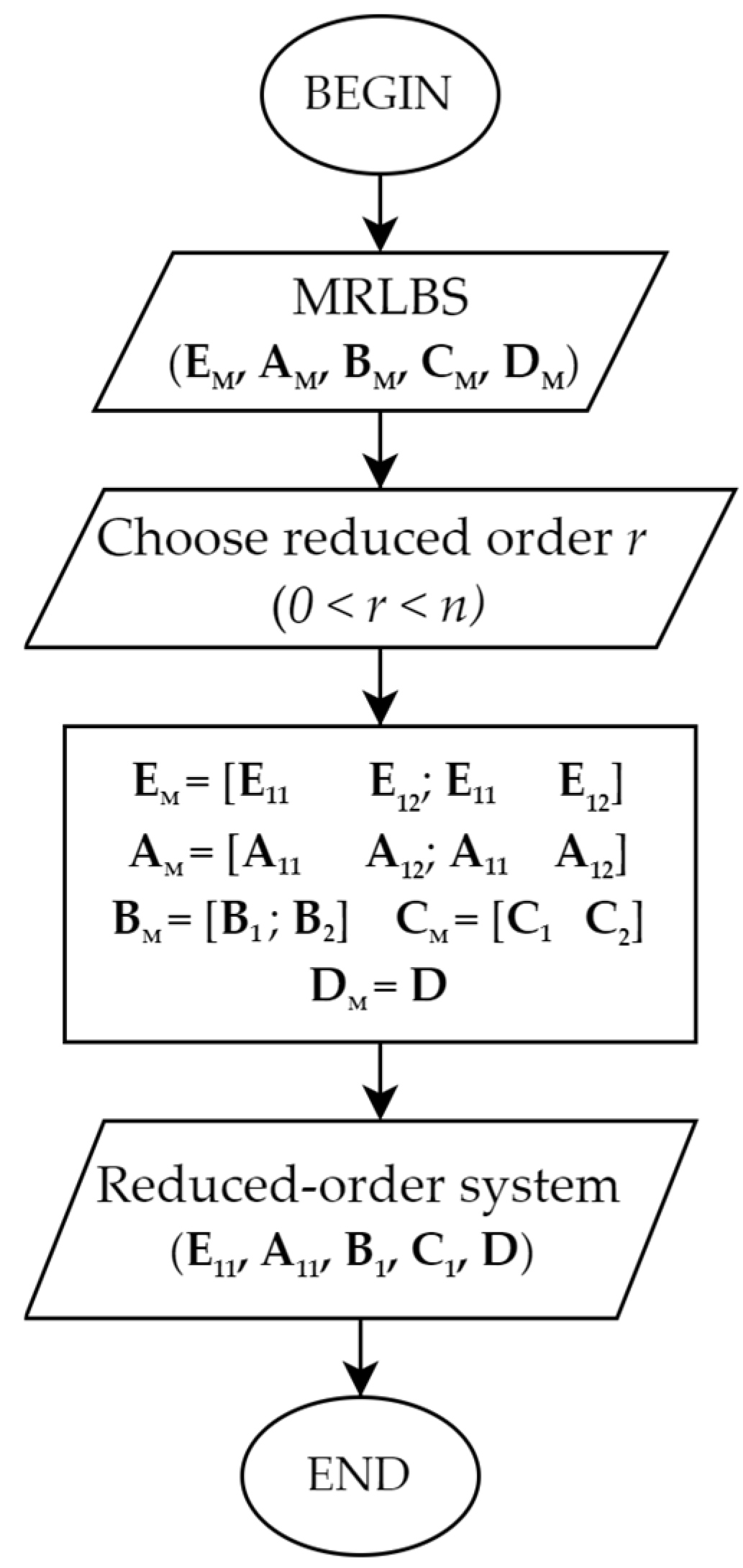
Algorithm Reduce model order using Mixed Riccati–Lyapunov Balanced Truncation (MRLBT) is depicted in Figure 2 and presented in Algorithm 2.
Algorithm 2. Reduce model order using Mixed Riccati–Lyapunov Balanced Truncation (MRLBT).
Input: The MRLBS ( E M , A M , B M , C M , D M ) .
  - Step 1. Choose the desired reduced-order r, where 0 < r < n.
  - Step 2. Represent the MRLBS matrices as block matrices as in (35).
E M = T - 1 E T = E 11 E 12 E 21 E 22 ; A M = T - 1 A n T = A 11 A 12 A 21 A 22 ; B M = T - 1 B n = B 1 B 2 ; C M = C n T = C 1 C 2 ; D M = D
  where:
   E 11 r × r , E 12 r × ( n r ) , E 21 ( n r ) × r , E 22 ( n r ) × ( n r ) ; A 11 r × r , A 12 r × ( n r ) , A 21 ( n r ) × r , A 22 ( n r ) × ( n r ) ; B 1 r × p , B 2 ( n r ) × p ; C 1 p × r , C 2 p × ( n r ) ; D p x p
Output: Reduced-order system ( E 11 , A 11 , B 1 , C 1 , D )
Theorem 5. 
The reduced-order system  ( E 11 , A 11 , B 1 , C 1 , D )  at the output of Algorithm 2 preserves the stability and passivity of the original LTI-CTD system (1).
Proof of Theorem 5. 
Equations (31) and (32) in block matrix form (38) and (39).
where:
M 1 = M 1 T = d i a g μ 1 , μ 2 , , μ r
M 2 = M 2 T = d i a g μ r + 1 , μ r + 2 , , μ n
A 11 A 12 A 21 A 22 M 1 0 0 M 2 E 11 E 12 E 21 E 22 T + E 11 E 12 E 21 E 22 M 1 0 0 M 2 A 11 A 12 A 21 A 22 T + B 1 B 2 B 1 B 2 T = 0
A 11 A 12 A 21 A 22 T M 1 0 0 M 2 E 11 E 12 E 21 E 22 + E 11 E 12 E 21 E 22 T M 1 0 0 M 2 A 11 A 12 A 21 A 22 + ( E 11 E 12 E 21 E 22 T M 1 0 0 M 2 B 1 B 2 C 1 C 2 T ) ( D + D T ) 1 × ( E 11 E 12 E 21 E 22 T M 1 0 0 M 2 B 1 B 2 C 1 C 2 T ) T = 0
Then the reduced-order system satisfies the Lyapunov Equation (40) and the positive-real Riccati Equation (41).
A 11 M 1 E 11 + E 11 M 1 A 11 T + B 11 B 11 T = 0
A 11 T M 1 E 11 + E 11 T M 1 A 11 + ( E 11 T M 1 B 1 C 1 T ) ( D + D T ) 1 ( E 11 T M 1 B 1 C 1 T ) T = 0
Since M1 is a diagonal, positive definite, symmetric matrix, satisfying Equations (12), (7), and Lemma 1, the reduced-order system in the output of Algorithm 2 preserves the stability and passivity of the original LTI-CTD system (1). □
Corollary 2. 
The reduced-order system  ( E 11 , A 11 , B 1 , C 1 , D )  at the output of Algorithm 2 satisfies Note 1, and its Gramian RLcr and Gramian RLor are diagonal, symmetric, positive definite matrices, containing r Hankel singular values of the original MRLBS (1): R L c r = R L o r = M 1 = M 1 T = d i a g m 1 , m 2 , , m r .
Proof of Corollary 2. 
From (36)–(39), what must be proven follows. □
Theorem 6. 
The LTI-CTD system (1), with the properties in Note 1, Lemma 1, and Definition 3 or which satisfies Theorem 4 (or Lemma 3) when reducing order using the MRLBT algorithm, has the upper limit of error as condition (42)
G ( s ) G M R L B T ( s ) H 2 r + 1 n μ i
Proof of Theorem 6. 
Expanding (7) we obtain Equation (43).
( A B ( D + D T ) 1 C ) T R o E + E T R o ( A B ( D + D T ) 1 C ) + E T R o B ( D + D T ) 1 B T C T ( D + D T ) 1 C = 0
According to (14) then, (43) has the form of Equation (44).
A n T R o E + E T R o A n + E T R o B n B n T R o E + C n T C n = 0
Cholesky decomposes E T R o B n B n T R o E + C n T C n to form (45).
E T R o B n B n T R o E + C n T C n = C m T C m
C m is the upper triangular matrix and is invertible.
The LTI-CTD system (1) is an MRLBS so R L c = R L o = M = d i a g μ 1 , μ 2 , , μ n , and (12) and (7) are transformed into two Equations (46) and (47), respectively.
A n M E T + E M A n T + B n B n T = 0
A n T M E + E T M A n + C m T C m = 0
These are two Lyapunov equations, so according to Definition 1 and Theorem 1, as well as according to the transformations and proofs in the BT algorithm, we have an error between the original system and the reduced-order system that satisfies Theorem 6. □

4. Illustrative Example

Considering that the RLC ladder network serves as a model for a transmission line, where the parameters R, L, and C are as in Figure 3 [34,35], with the number of nodes k = 8, and the order of this electrical network model is n = 15. The state variables x2j−1 are the voltage across Cjx2i is the current flowing through Liu is the input voltage, and y is the output current.
Applying the Modified Nodal Analysis (MNA) technique to the electrical circuit as shown in Figure 3 along with the given parameters, we obtain the system matrices as in Equation (48).
E = I 15 × 15 ; A = A 1 0 7 × 7 0 7 × 7 A 2 ; B = [ 0 1 × 14 5 ] T ;   C = [ 0 1 × 14 5 ] ;   D = 5
where I15×15 is the identity matrix of size 15 × 15, 07×7 is a zero matrix of size 7 × 7, and 01×14 is a zero matrix of size 1 × 4;
A 1 = 3 1 0 0 0 0 0 0 1 0 1 0 0 0 0 0 0 1 1 1 0 0 0 0 0 0 1 0 1 0 0 0 0 0 0 1 1 1 0 0 0 0 0 0 1 0 1 0 0 0 0 0 0 1 1 1 0 0 0 0 0 0 1 0 ; A 2 = 1 1 0 0 0 0 0 0 1 0 1 0 0 0 0 0 0 1 1 1 0 0 0 0 0 0 1 0 1 0 0 0 0 0 0 1 1 1 0 0 0 0 0 0 1 0 1 0 0 0 0 0 0 1 1 1 0 0 0 0 0 0 1 6
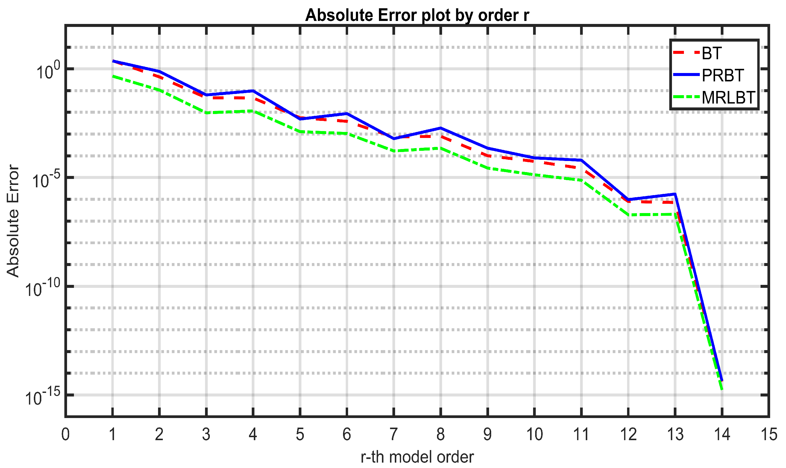
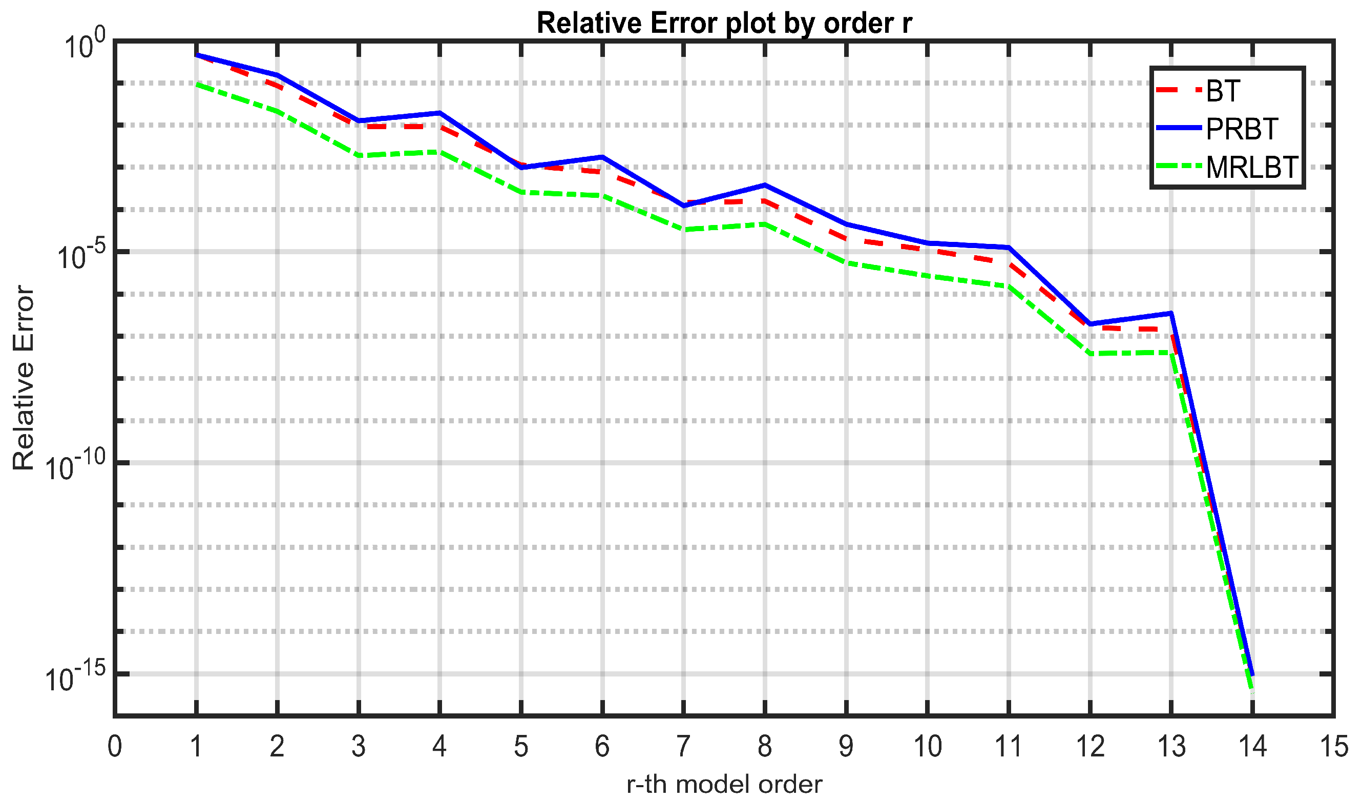
Implementing the BT, PRBT, and MRLBT algorithms in Matlab 2023b to reduce the order of this model from order r = 15 to order r = 1, for each model order r, we obtain absolute and relative errors as shown in Table 1 and Table 2. The plots of these errors are presented accordingly in Figure 4 and Figure 5.
From Table 1 and Table 2 and Figure 4 and Figure 5, along with the numerical data and visual representations, several observations can be made:
-
The error diminishes as the order decreases when applying all three algorithms, which aligns with theoretical expectations. As the model’s order decreases, its quality improves, resulting in smaller errors.
-
Across all orders r, the error between the original system and the reduced-order system using MRLBT is the smallest, followed by BT, with PRBT yielding the largest error.
-
When r ≥ 5, the error between the original and reduced-order systems approaches zero consistently across all three algorithms.
The Hankel Singular Values (HSV) of this transmission line model, when transformed into a Mixed Riccati–Lyapunov Balanced System, are presented in Table 3.
In Table 3, it is observed that the HSV of an MRLBS gradually decreases as the order r increases. This observation is consistent with theory and practice, since a smaller HSV implies less loss of information from the original system, leading to a corresponding increase in the reduction error as the system is reduced.
Examining Table 3 alongside the upper bound estimation formula for the error reduction provided by the MRLBT algorithm in Equation (42), the upper limit values of the proposed error are derived in Table 1’s “Proposed Error” column. When comparing these estimated errors with the actual errors obtained under the column “MRLBT Error” in Table 1, it is evident that the formula proposed in Theorem 6 is entirely feasible.
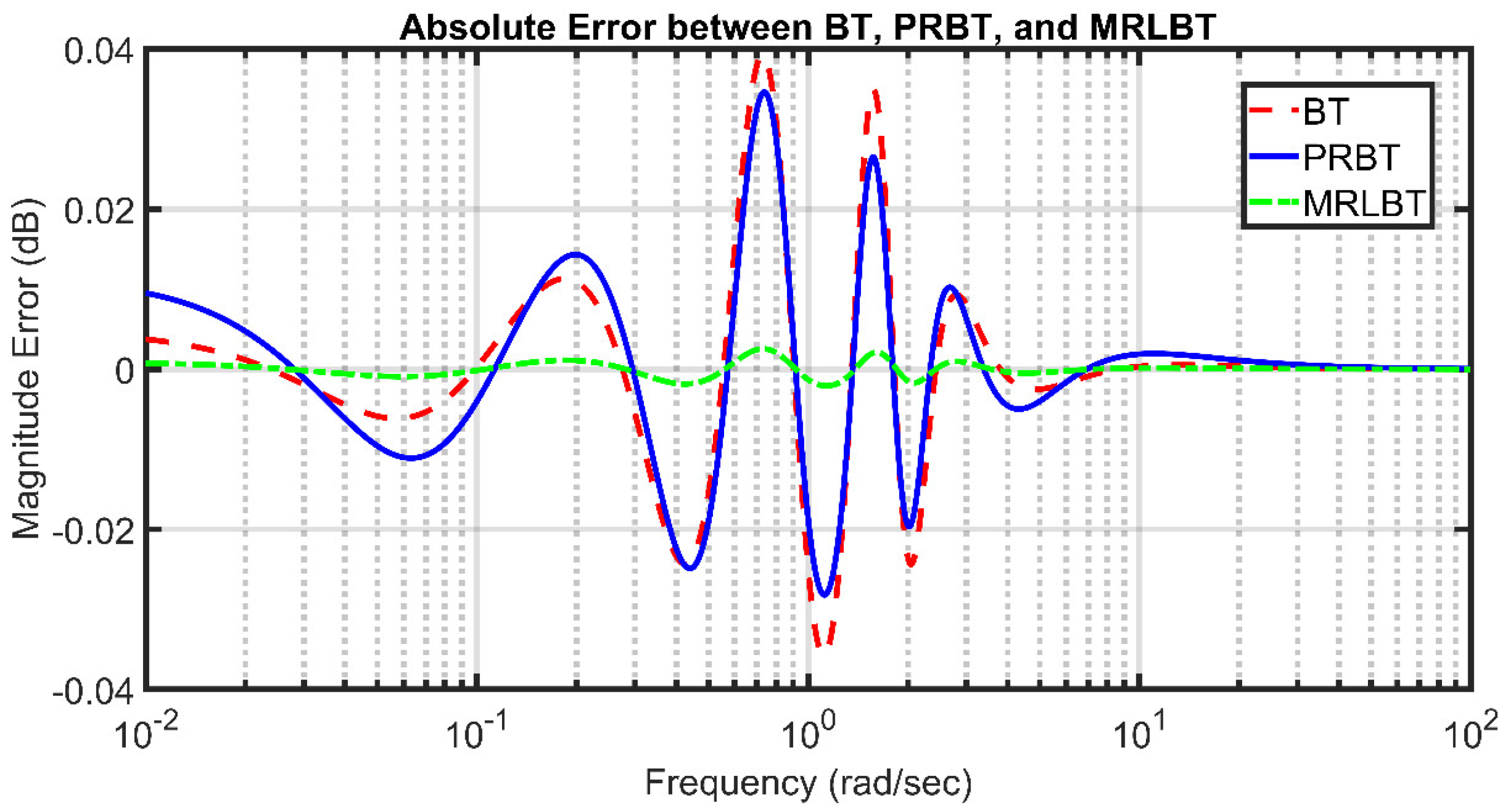
Considering the case of reducing the system to order r = 5 using the BT, PRBT, and MRLBT algorithms, we proceed to compare the Magnitude and Phase errors in the frequency domain and the Magnitude errors in the time domain. The results are illustrated in Figure 6, Figure 7 and Figure 8.
From the Magnitude and Phase error plots in the frequency domain (Figure 6 and Figure 7), it is observed that across the entire frequency range (from 10−2 Rad/s to 102 Rad/s), the MRLBT algorithm yields the best reduction in error, with very small discrepancies. BT and PRBT exhibit larger deviations from the original system. Beyond 102 Rad/s, all three algorithms show similar errors, approaching zero.
Similarly, in the Magnitude error plot in the time domain (Figure 8), the model reduced to order 5 using the MRLBT algorithm demonstrates the smallest error, while PRBT still exhibits the largest error. All three algorithms show increasing Magnitude discrepancies over time.
The 15th-order system G with reduced-order systems were analyzed to the 5th order using the PRBT, BT, and MRLBT algorithms, denoted as G_PRBT, G_BT, and G_MRLBT respectively, based on certain parameters: Transient Time (s), Settling Time (s), Settling Min (s), and Overshoot (s), as shown in Table 4.
In Table 4, “Transient Time” represents the time taken for the system’s response to settle within a specified error band, “Settling Time” indicates the time required for the system’s response to settle within a specified percentage of the final value, “Settling Min” refers to the minimum value reached by the system during settling, and “Overshoot” shows the percentage by which the system’s response exceeds the final value before settling. Based on these values, we have observations, assessments, and comparisons of the results:
-
Transient Time: System G_MRLBT exhibits the shortest transient time among all systems, indicating the fastest response to input changes. Systems G, G_PRBT, and G_BT have slightly longer transient times, suggesting slightly slower responses compared to G_MRLBT.
-
Settling Time: G_MRLBT achieves the fastest settling time, indicating quicker stabilization compared to the other systems. G, G_PRBT, and G_BT have similar settling times, which are notably longer than that of G_MRLBT.
-
Settling Min: G_MRLBT has the highest minimum settling value, indicating a more stable settling process compared to the other systems. G, G_PRBT, and G_BT have similar minimum settling values, which are notably lower than that of G_MRLBT.
-
Overshoot: G_MRLBT exhibits significantly lower overshoot compared to the other systems, suggesting a more controlled response. G, G_PRBT, and G_BT show similar levels of overshoot, which are substantially higher compared to G_MRLBT.
→ G_MRLBT demonstrates superior performance across all metrics, showing faster response times, quicker settling, higher stability, and lower overshoot compared to G, G_PRBT, and G_BT. This indicates that the modified robust loop-based tuning approach (G_MRLBT) potentially offers better control and stability characteristics compared to the other tuning methods evaluated.
Overall evaluation: The MRLBT algorithm demonstrates a significant advantage over BT and PRBT. This indicates that MRLBT is a preferable option for reducing the order of electrical and electronic circuit models. From the illustrated example, the simulation results align well with the theoretical foundation and the mathematical reasoning provided. This reaffirms that the proposed MRLBT reduction algorithm works as expected and achieves its intended goals.

5. Analysis and Discussion

5.1. Special Case of Matrix D = 0

In the special case where the system (1) has a D matrix equal to 0, as illustrated in the example of the RLC ladder network in Section 4, if RS is extremely large, meaning D = [1/RS] ≈ [0], then transformation (14) cannot be applied because F becomes non-invertible.
In this scenario, still adhering to the algorithmic approach, we proceed to determine the controllability Gramian matrix P from the Lyapunov Equation (2), and the observability Gramian matrix Ro obtained from Lemma 1 in Equation (10). Subsequently, we verify whether these two Gramian matrices satisfy Definition 3, i.e., P = Ro. If so, MRLBT can be implemented to reduce the model order following the steps outlined in Algorithm 2. If Definition 3 is not satisfied, Algorithm 1 is executed first, followed by the application of MRLBT. It is noted that in this case, Lc = P and Ro are not determined from (13) but from (10), specifically R o = E T C T B 1 .

5.2. Comparative Analysis of MRLBT with BT and PRBT

-
Comparison of MRLBT with BT and PRBT:
+
MRLBT utilizes a Lyapunov equation to determine the controllability Gramian, akin to BT, and employs a positive definite Riccati equation to determine the observability Gramian, akin to PRBT.
+
MRLBT preserves stability similar to BT and PRBT, as well as passive properties akin to PRBT.
+
Balanced Truncation Techniques: MRLBT, PRBT, and BT all utilize balanced truncation techniques as part of their reduction process. These techniques involve balancing the controllability and observability Gramians of the original system to identify the most significant system modes for retention in the reduced-order model.
+
Focus on Stability and Accuracy: All three methods prioritize stability and accuracy in the reduced-order model. They aim to retain the essential dynamics of the original system while discarding less significant modes to achieve computational efficiency without sacrificing model fidelity.
-
Advantages of MRLBT over BT and PRBT:
+
MRLBT incurs lower computational cost compared to PRBT, as it solves only one positive definite Riccati equation instead of two as in PRBT.
+
BT fails to preserve passive properties unlike MRLBT.
+
The reduction error of MRLBT is smaller than that of BT and PRBT.

5.3. Description of the Methodology of Using MRLBT for Electrical Engineering

Firstly, a system model in the form of (1) with the characteristics outlined in Note 1 is required. To obtain the dynamic representation (1), one can employ benchmark models of electrical circuits, electronics, or apply the Modified Nodal Analysis (MNA) technique to convert the circuit schematic into mathematical form (1).
Once a model in the LTI-CTD form is obtained, if the system satisfies Definition 3, Algorithm 2 (MRLBT algorithm) can be directly applied to reduce the model order.
In cases where the system (1) does not satisfy Definition 3, Algorithm 1 is applied to transform it into an equivalent MRLBS form. This transformation ensures the preservation of stability and passivity, critical properties of electrical circuits.
The transformation process involves solving Lyapunov equations to obtain the controllability and observability Gramian matrices, which are essential for determining the balanced form of the system. Additionally, a non-singular transformation matrix is computed to bring the original system into the balanced form.
Once the system is in the MRLBS form, the reduction process can commence. This involves selecting the desired reduced order and representing the MRLBS matrices as block matrices.
Finally, the reduced-order system is obtained by applying the MRLBT algorithm, which ensures that the stability and passivity of the original system are preserved in the reduced model.
The selection of the reduced order can be based on criteria such as: the reduced-order system having an absolute (or relative) error smaller than a specified threshold, or the response of the reduced-order system in the time domain, frequency domain, phase angle, or magnitude satisfying an application requirement, or preserving certain Hankel singular values of the system in the reduced-order model, etc.

5.4. Approaches Related to the Software and Practical Implementation of MRLBT

Practical implementation of the MRLBT algorithm involves translating the theoretical concepts into software code. This can be done using programming languages like MATLAB, Python 2.x and above versions, or other computational software tools.
The implementation typically consists of functions or scripts that perform the following tasks: Computing the controllability and observability Gramian matrices. Performing Cholesky decomposition and singular value decomposition to obtain the transformation matrix. Applying the transformation to convert the original system into the Mixed Riccati–Lyapunov balanced form. Selecting the desired reduced order and representing the system matrices as block matrices.
In addition to the algorithmic implementation, practical considerations such as computational efficiency and numerical stability should be taken into account, to ensure its correctness and reliability.

5.5. Error Analysis and Error Minimization Strategies for MRLBT

Improving the accuracy of the high-order model via advanced system identification techniques can mitigate modeling errors and enhance the precision of the reduced-order model.
Employing sophisticated algorithms or heuristics to ascertain the optimal reduced order according to predefined criteria, such as error bounds or system performance requirements, can mitigate errors while managing computational expenses.
Adopting more precise methods for approximating the controllability and observability Gramian matrices can mitigate errors linked to Gramian approximation.
Formulating strategies to better balance the controllability and observability Gramians can refine reduction accuracy and diminish error.
Utilizing the highest precision data types of numerical tools for improved approximation, employing novel algorithms to optimize matrix computations, equation solving procedures, mathematical transformations to minimize errors at each data processing step.
During the reduction process, additional optimization algorithms such as Slime Mould Algorithm, Simulated Annealing, Genetic Algorithm, Particle Swarm Optimization, Ant Colony Optimization, etc., can be integrated to compensate for errors, minimize reduction errors, or ensure that the reduced-order system closely follows the original system’s step response and Bode plot while preserving the physical properties of the original system, such as stability and passivity.

5.6. Limitations of the MRLBT Algorithm

MRLBT is primarily designed for Linear Time-Invariant Continuous-Time Descriptor Systems (LTI-CTD) that satisfy the properties in Note 1 and may not directly address present real-world electrical engineering problems.
The applicability of MRLBT may be limited to certain types of systems or scenarios. It may not be suitable for systems with highly nonlinear dynamics, unstable systems, or for cases where certain assumptions underlying the algorithm are violated.

6. Conclusions

This paper has presented a novel order reduction algorithm, termed Mixed Riccati–Lyapunov Balanced Truncation (MRLBT), tailored for Linear Time-Invariant Continuous-Time Descriptor Systems (LTI-CTD) prevalent in electrical and electronic circuit modeling. The MRLBT algorithm combines the advantages of balanced truncation (BT) and positive-real balanced truncation (PRBT) while addressing their respective limitations. Through theoretical analysis and mathematical proofs, it has been shown that MRLBT guarantees the preservation of stability and passivity inherent in the original system, a crucial requirement for electrical circuit models. Additionally, MRLBT achieves reduced computational complexity and minimized order reduction errors compared to PRBT. The efficacy of MRLBT has been demonstrated through a numerical example involving an RLC ladder network, representing a transmission line model. The simulation results have validated the theoretical foundations and showcased the superior performance of MRLBT over BT and PRBT in terms of reduced errors in both the time and frequency domains.
Overall, the proposed MRLBT algorithm presents a promising approach for order reduction of electrical and electronic circuit systems, enabling the development of computationally efficient and reliable reduced-order models while preserving critical physical properties. Future research directions may explore extending the MRLBT methodology to non-linear and time-varying systems, as well as investigating its applications in control system design and optimization.

Author Contributions

Conceptualization, H.-D.D.; Methodology, H.-D.D.; Software, T.-T.N. and H.-S.V.; Validation, N.-K.V. and H.-S.V.; Formal analysis, N.-K.V. and H.-Q.N.; Investigation, T.-T.N.; Resources, N.-K.V.; Data curation, T.-T.N., N.-K.V. and H.-S.V.; Writing—original draft, T.-T.N.; Writing—review & editing, N.-K.V.; Supervision, H.-Q.N.; Project administration, H.-Q.N.; Funding acquisition, H.-D.D. All authors have read and agreed to the published version of the manuscript.

Funding

This research was financially supported by the Program of the Ministry of Education and Training of Vietnam under grant number B2023-TNA-17.

Data Availability Statement

The data presented in this study are available in the present article.

Conflicts of Interest

The authors declare no conflicts of interest.

References

  1. Choupanzadeh, R.; Zadehgol, A. Blockwise vs. and General MNA for MOR. In Proceedings of the 2023 IEEE International Symposium on Antennas and Propagation and USNC-URSI Radio Science Meeting (USNC-URSI), Portland, OR, USA, 23–28 July 2023; pp. 847–848. [Google Scholar]
  2. Hao, L.; Shi, G. Realizable Reduction of Multi-Port RCL Networks by Block Elimination. IEEE Trans. Circuits Syst. I Regul. Pap. 2023, 70, 399–412. [Google Scholar] [CrossRef]
  3. Pavan, S.; Temes, G.C. Reciprocity and inter-reciprocity: A tutorial—Part I: Linear time-invariant networks. IEEE Trans. Circuits Syst. I Regul. Pap. 2023, 70, 3413–3421. [Google Scholar] [CrossRef]
  4. Benner, P. System- and Data-Driven Methods and Algorithms; De Gruyter: Berlin, Germany, 2021. [Google Scholar]
  5. Freund, R.W. Electronic Circuit Simulation and the Development of New Krylov-Subspace Methods. In Novel Mathematics Inspired by Industrial Challenges; Springer International Publishing: Cham, Switzerland, 2022; pp. 29–55. [Google Scholar]
  6. Liu, S.-M.; Jiang, L.-J.; Li, P. A Fast AWE-Augmented Wideband Discontinuous Galerkin Frequency-Domain Method in Solving Electromagnetic Wave Equations. In Proceedings of the 2022 IEEE International Symposium on Antennas and Propagation and USNC-URSI Radio Science Meeting (AP-S/URSI), Denver, CO, USA, 10–15 July 2022. [Google Scholar]
  7. Bhattacharya, A.; Nandy, P.; Nath, P.P.; Sahu, H. On Krylov complexity in open systems: An approach via bi-Lanczos algorithm. J. High Energy Phys. 2023, 12, 1–30. [Google Scholar] [CrossRef]
  8. Prajapati, A.K.; Prasad, R. Model reduction using the balanced truncation method and the Padé approximation method. IETE Tech. Rev. 2022, 39, 257–269. [Google Scholar] [CrossRef]
  9. Khattak, M.A.; Romano, D.; Antonini, G.; Ferranti, F. Efficient Frequency and Time-Domain Simulations of Delayed PEEC Models With Proper Orthogonal Decomposition Techniques. IEEE Access 2024, 12, 168–178. [Google Scholar] [CrossRef]
  10. Wang, G.; Yang, J.; Jiao, J. Voltage correlation-based principal component analysis method for short circuit fault diagnosis of series battery pack. IEEE Trans. Ind. Electron. 2022, 70, 9025–9034. [Google Scholar] [CrossRef]
  11. Vuillemin, P.; Maillard, A.; Poussot-Vassal, C. Optimal modal truncation. Syst. Control Lett. 2021, 156, 105011. [Google Scholar] [CrossRef]
  12. Ali, H.R.; Kunjumuhammed, L.P.; Pal, B.C.; Adamczyk, A.G.; Vershinin, K. Model Order Reduction of Wind Farms: Linear Approach. IEEE Trans. Sustain. Energy 2019, 10, 1194–1205. [Google Scholar] [CrossRef]
  13. Freitas, F.D.; Rommes, J.; Martins, N. Developments in the Computation of Reduced Order Models with the Use of Dominant Spectral Zeros. In Realization and Model Reduction of Dynamical Systems: A Festschrift in Honor of the 70th Birthday of Thanos Antoulas; Springer International Publishing: Cham, Switzerland, 2022; pp. 215–233. [Google Scholar]
  14. Moore, B. Principal component analysis in linear systems: Controllability, observability, and model reduction. IEEE Trans. Autom. Control 1981, 26, 17–32. [Google Scholar] [CrossRef]
  15. Benner, P.; Du, X.; Yang, G.; Ye, D. Balanced truncation of linear time-invariant systems over finite-frequency ranges. Adv. Comput. Math. 2020, 46, 1–34. [Google Scholar] [CrossRef]
  16. König, J.; Freitag, M.A. Time-Limited Balanced Truncation for Data Assimilation Problems. J. Sci. Comput. 2023, 97, 47. [Google Scholar] [CrossRef]
  17. Wu, J.-L.; Yung, C.-F.; Liu, W.-T. A new bounded real lemma for discrete-time linear descriptor systems. Asian J. Control 2023, 26, 1068–1076. [Google Scholar] [CrossRef]
  18. Tan, S.; He, L. Advanced Model Order Reduction Techniques in VLSI Design; Cambridge University Press: Cambridge, UK, 2007. [Google Scholar]
  19. Becker, S.; Hartmann, C. Infinite-dimensional bilinear and stochastic balanced truncation with explicit error bounds. Math. Control Signals Syst. 2019, 31, 1–37. [Google Scholar] [CrossRef]
  20. Damm, T.; Redmann, M. Complexity reduction of large-scale stochastic systems using linear quadratic Gaussian balancing. J. Franklin Inst. 2023, 360, 14534–14552. [Google Scholar] [CrossRef]
  21. Raja, C.V.N.; Surendra, P. Design of H-infinity controller for a reduced order linearized power electronic cricuit. J. Electr. Eng. 2020, 20, 9. [Google Scholar]
  22. Benner, P.; Werner, S.W.R. Hankel-norm approximation of large-scale descriptor systems. Adv. Comput. Math. 2020, 46, 40. [Google Scholar] [CrossRef]
  23. Antoulas, A.C. Approximation of Large-Scale Dynamical Systems; Society for Industrial and Applied Mathematics: Philadelphia, PA, USA, 2005. [Google Scholar]
  24. Mehrmann, V.; Stykel, T. Balanced truncation model reduction for large-scale systems in descriptor form. In Dimension Reduction of Large-Scale Systems: Proceedings of a Workshop Held in Oberwolfach, Germany, October 19–25, 2003; Springer: Berlin/Heidelberg, Germany, 2005. [Google Scholar]
  25. Reis, T.; Stykel, T. Positive real and bounded real balancing for model reduction of descriptor systems. Int. J. Control 2010, 83, 74–88. [Google Scholar] [CrossRef]
  26. Benner, P.; Stykel, T. Model Order Reduction for Differential-Algebraic Equations: A Survey. In Surveys in Differential-Algebraic Equations IV; Ilchmann, A., Reis, T., Eds.; Differential-Algebraic Equations Forum; Springer: Cham, Switzerland, 2017. [Google Scholar]
  27. Unneland, K.; Van Dooren, P.; Egeland, O. New Schemes for Positive Real Truncation. Model. Identif. Control A Norw. Res. Bull. 2007, 28, 53–65. [Google Scholar] [CrossRef]
  28. Phillips, J.R.; Daniel, L.; Silveira, L.M. Guaranteed passive balancing transformations for model order reduction. IEEE Trans. Comput.-Aided Des. Integr. Circuits Syst. 2003, 22, 1027–1041. [Google Scholar] [CrossRef]
  29. Unneland, K.; Van Dooren, P.; Egeland, O. A Novel Scheme for Positive Real Balanced Truncation. In Proceedings of the 2007 American Control Conference, New York, NY, USA, 9–13 July 2007; pp. 947–952. [Google Scholar]
  30. Zulfiqar, U.; Tariq, W.; Li, L.; Liaquat, M. A Passivity-Preserving Frequency-Weighted Model Order Reduction Technique. IEEE Trans. Circuits Syst. II Express Briefs 2017, 64, 1327–1331. [Google Scholar] [CrossRef]
  31. Zulfiqar, U.; Imran, M.; Ghafoor, A.; Liaqat, M. Time/frequency-limited positive-real truncated balanced realizations. IMA J. Math. Control Inf. 2020, 37, 64–81. [Google Scholar] [CrossRef]
  32. Stefanovski, J. Kalman–Yakubovič–Popov lemma for descriptor systems. Syst. Control Lett. 2014, 74, 8–13. [Google Scholar] [CrossRef]
  33. Iwasaki, T. KYP Lemma and Generalizations/Applications. In Encyclopedia of Systems and Control; Baillieul, J., Samad, T., Eds.; Springer: Cham, Switzerland, 2021. [Google Scholar]
  34. Saadvandi, M. Passivity Preserving Model Reduction and Selection of Spectral Zeros. Master’s Thesis, Royal Institute of Technology KTH, Stockholm, Sweden, 2008. [Google Scholar]
  35. Antoulas, A.C.; Ionutiu, R.; Martins, N.; ter Maten, E.J.W.; Mohaghegh, K.; Pulch, R.; Rommes, J.; Saadvandi, M.; Striebel, M. Model order reduction: Methods, concepts and properties. In Coupled Multiscale Simulation and Optimization in Nanoelectronics; Springer: Berlin/Heidelberg, Germany, 2015; pp. 159–265. [Google Scholar]
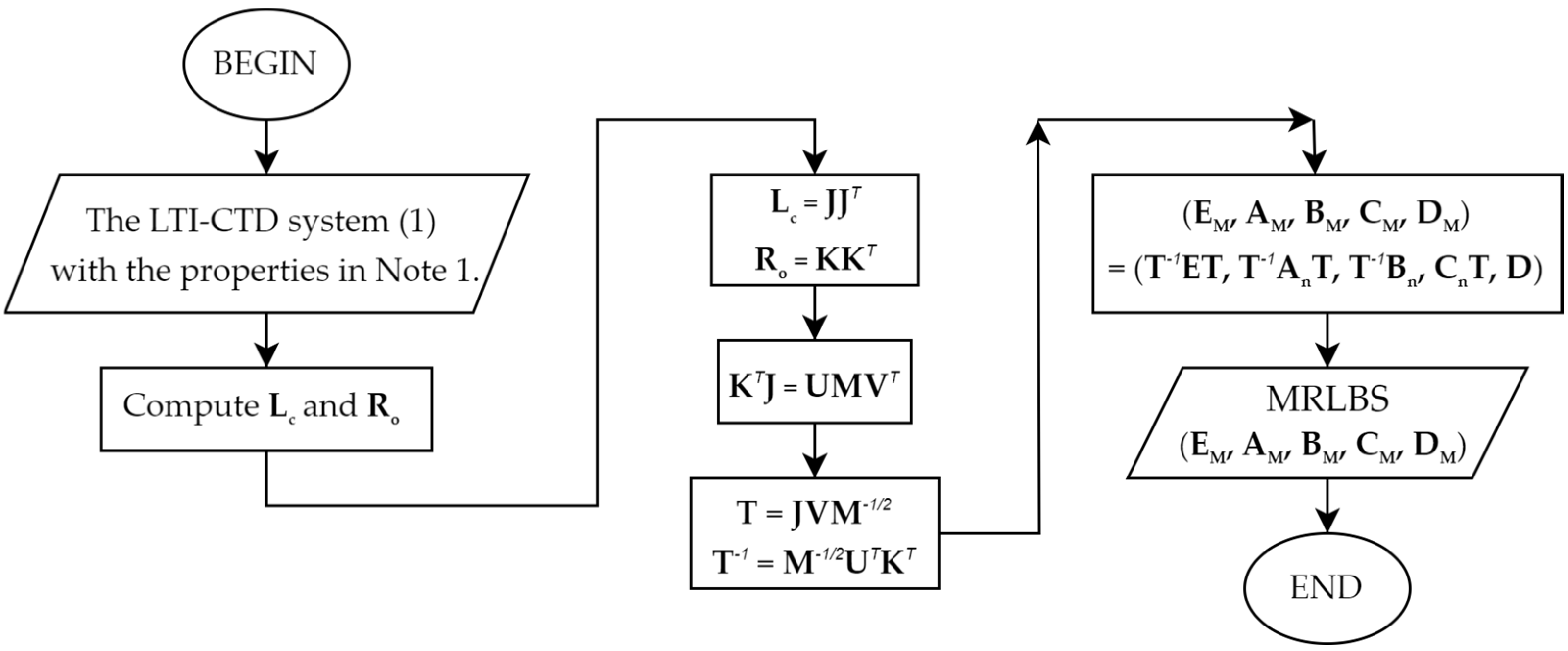
Figure 1. Flowchart of Algorithm 1.
Energies 17 02661 g001
Figure 2. Flowchart of Algorithm 2.
Energies 17 02661 g002
Figure 3. RLC ladder network with n order.
Energies 17 02661 g003
Figure 4. Corresponding absolute error plot according to r-th order.
Energies 17 02661 g004
Figure 5. Corresponding relative error plot according to r-th order.
Energies 17 02661 g005
Figure 6. Magnitude error when model order reduced using BT, PRBT, and MRLBT.
Energies 17 02661 g006
Figure 7. Phase error when model order reduced using BT, PRBT, and MRLBT.
Energies 17 02661 g007
Figure 8. Absolute error in amplitude when model order reduced using BT, PRBT, and MRLBT.
Energies 17 02661 g008
Table 1. Absolute errors of the BT, PRBT, and MRLBT algorithms, and proposed error bound.
Order rAbEBTAbEPRBTAbEMRLBT(AbEMRLBT/AbEBT)%(AbEMRLBT/AbEPRBT)%Proposed Error
123.78220 × 10−123.15991 × 10−14.643264 × 10−119.52411520.048715.496241 × 10−1
24.266310 × 10−17.612429 × 10−11.059499 × 10−124.83408413.918011.369536 × 10−1
34.681724 × 10−26.319774 × 10−20.9515981 × 10−220.32580515.057473.550382 × 10−2
44.583141 × 10−29.715357 × 10−21.163701 × 10−225.39090511.977951.555651 × 10−2
55.654912 × 10−34.922613 × 10−31.289766 × 10−322.80788826.200843.180862 × 10−3
63.866860 × 10−38.780551 × 10−31.068293 × 10−327.62688612.166581.577823 × 10−3
77.330208 × 10−46.161054 × 10−41.672907 × 10−422.82209527.152944.904308 × 10−4
87.915596 × 10−418.98488 × 10−42.246624 × 10−428.38224711.833752.639496 × 10−4
910.10776 × 10−522.49021 × 10−52.733811 × 10−527.04665512.155566.256161 × 10−5
105.566608 × 10−58.014040 × 10−51.342566 × 10−524.11820616.752672.535941 × 10−5
1126.68909 × 10−663.19410 × 10−67.550555 × 10−628.29079211.94828.352720 × 10−6
127.920579 × 10−79.672938 × 10−71.945731 × 10−724.56551520.11525.337477 × 10−7
137.153312 × 10−717.45577 × 10−72.051143 × 10−728.67403211.750522.116865 × 10−7
144.160653 × 10−154.424140 × 10−151.708269 × 10−1541.05771438.612452.342412 × 10−9
Table 2. Relative errors of the BT, PRBT, and MRLBT algorithms.
Order rReEBTReEPRBTReEMRLBT(ReEMRLBT/ReEBT)%(ReEMRLBT/ReEPRBT)%
14.756440 × 10−14.631982 × 10−10.9286528 × 10−119.52411520.04871
28.532620 × 10−215.22486 × 10−22.118998 × 10−224.83408413.91801
39.363448 × 10−312.63955 × 10−31.903196 × 10−320.32580315.05747
49.166282 × 10−319.43071 × 10−32.327401 × 10−325.39089511.97795
511.30982 × 10−49.845227 × 10−42.579532 × 10−422.80789626.20084
67.733720 × 10−417.56110 × 10−42.136586 × 10−427.62688612.16658
714.66042 × 10−512.32211 × 10−53.345814 × 10−522.82208827.15293
815.83119 × 10−537.96976 × 10−54.493248 × 10−528.38225011.83375
920.21553 × 10−644.98042 × 10−65.467622 × 10−627.04664212.15556
1011.13322 × 10−516.02808 × 10−62.685133 × 10−624.11820716.75268
115.337817 × 10−612.63882 × 10−61.510111 × 10−628.29079811.9482
1215.84116 × 10−819.34588 × 10−83.891463 × 10−824.56551820.1152
1314.30662 × 10−834.91154 × 10−84.102287 × 10−828.67404711.75052
148.321307 × 10−168.848280 × 10−163.416538 × 10−1641.05770938.61245
Table 3. HSV of the RLC ladder network when converted to an MRLBS.
μiHSV of MRLBSμiHSV of MRLBS
13.5536 × 10−191.0069 × 10⁻⁴
22.0634 × 10−1101.8601 × 10−5
35.0725 × 10−2118.5033 × 10−6
49.9737 × 10−3123.9095 × 10−6
56.1878 × 10−3131.6103 × 10−7
68.0152 × 10−4141.0467 × 10−7
75.4370 × 10−4151.1712 × 10−9
81.1324 × 10⁻⁴
Table 4. Comparison of performance metrics for systems G, G_PRBT, G_BT, and G_MRLBT.
ParameterGG_PRBTG_BTG_MRLBT
Transient Time (s)62.7962.1362.4148.71
Settling Time (s)55.6355.0455.3015.65
Settling Min (s)1.141.141.144.39
Overshoot (s)50.0050.2050.084.18
Disclaimer/Publisher’s Note: The statements, opinions and data contained in all publications are solely those of the individual author(s) and contributor(s) and not of MDPI and/or the editor(s). MDPI and/or the editor(s) disclaim responsibility for any injury to people or property resulting from any ideas, methods, instructions or products referred to in the content.