Article

Modeling Wind-Speed Statistics beyond the Weibull Distribution

1
Department of Computer Science, OsloMet–Oslo Metropolitan University, N-0130 Oslo, Norway
2
Artificial Intelligence Lab, Oslo Metropolitan University, N-0166 Oslo, Norway
3
NordSTAR–Nordic Center for Sustainable and Trustworthy AI Research, Pilestredet 52, N-0166 Oslo, Norway
4
Simula Research Laboratory, Numerical Analysis and Scientific Computing, N-0164 Oslo, Norway
*
Author to whom correspondence should be addressed.
Energies 2024, 17(11), 2621; https://doi.org/10.3390/en17112621
Submission received: 6 May 2024 / Revised: 25 May 2024 / Accepted: 28 May 2024 / Published: 29 May 2024
(This article belongs to the Special Issue Recent Development and Future Perspective of Wind Power Generation)

Abstract

:
While it is well known that the Weibull distribution is a good model for wind-speed measurements and can be explained through simple statistical arguments, how such a model holds for shorter time periods is still an open question. In this paper, we present a systematic investigation of the accuracy of the Weibull distribution to wind-speed measurements, in comparison with other possible “cousin” distributions. In particular, we show that the Gaussian distribution enables one to predict wind-speed histograms with higher accuracy than the Weibull distribution. Two other good candidates are the Nakagami and the Rice distributions, which can be interpreted as particular cases of the Weibull distribution for particular choices of the shape and scale parameters. These findings hold not only when predicting next-point values of the wind speed but also when predicting the wind energy values. Finally, we discuss such findings in the context of wind power forecasting and monitoring for power-grid assessment.

1. Introduction: What Is the Model Underlying Wind-Speed Distributions?

Historically, sets of wind-speed measurements have been modeled as a two-parameter distribution, the so-called Weibull distribution [1], since it follows from simple statistical assumptions, as we briefly explain below. However, although this model has been found to be the most appropriate [2], being used in the large majority of studies [3], recent studies have pointed towards other alternative models, such as the inverse Weibull distribution and the Rayleigh distribution, which show stronger accuracy to fit wind-speed distributions in some cases [4,5,6]. For example, in Ref. [2] the authors develop a system of wind-speed distributions able to retrieve the main statistical features of wind-speed regimes, combining statistical models with machine-learning implementations. Modeling distributions of stochastic variables have also been addressed in other contexts, namely in finance to assess the non-stationary evolution of volume-price in the stock market [7].
An accurate model for the distribution of wind-speed measurements is important in the present conjuncture of energy transfer strategies from conventional to renewable energy sources [8,9], since the dynamical features, including the high fluctuations and turbulent character of the wind speed, are reflected in the power output of wind turbines [10,11,12] and, consequently, in the economical viability of renewable energy strategies in many countries [13,14,15,16,17]. Models for the distributions of wind-speed measurements are fundamental to estimate the power output of wind turbines [18] and in the application of mathematical and artificial-intelligence methods to power-grid modeling and monitoring [19]. In particular, wind-speed fluctuations have been modeled with auto-regressive integrated moving average (ARIMA) models [20] to reproduce heavy-tail features of power output. Moreover, approaches derived from statistical physics out of equilibrium were proposed to derive deterministic and stochastic contributions in wind-speed time-series, handling wind speed as a stochastic process [21,22,23], which can then be used to assess the power performance of wind turbines [11,24] and to model short-time fluctuations [25] as well as 10-min average wind power curves [12], wind turbine vibrations [26], torque [27], and fatigue loads [28].
The purpose of this paper is to present a systematic investigation of a family of two-parameter distributions of wind speeds measured over different time-periods, spanning from 10-min to one-month windows. As an overall outcome, we show that while the Weibull distribution is a good model for large time windows, the simple Gaussian distribution as well as particular variants of the Weibull distribution, namely the Nakagami and the Rician distributions, show better goodness-of-fit for short time windows. We begin in Section 2 by presenting the main models and methods and describing the data from FINO-1. In Section 3, we present the main results, which are then discussed in Section 4, which also presents the main conclusions of the paper.

2. Models, Methods, and Data

2.1. Wind Data Measured at FINO-1 Tower at the North Sea

Our analysis is carried out with data from the FINO-1 platform, located at the North Sea, within Alpha Ventus, a wind farm with 12 wind turbines used for research in wind energy production and wind energy systems; see Figure 1. FINO stands for Forschungsplattformen in Nord- und Ostsee and comprises three research platforms, funded by the Federal Ministry for Economic Affairs and Energy (BMWi), with the aim of reducing wind energy costs and providing more reliable operation procedures for wind turbines.
The datasets comprise 1 Hz wind-speed measurements collected at the Offshore Research Platfrom FINO-1 located in the North Sea, approximately 45 km north of the German island of Borkum (N 54° 00 53.5 , E 6° 35 15.15 ). As shown in Figure 1 (left), FINO-1 is located in the immediate vicinity of the wind farm Alpha Ventus. The dataset spans three years and is collected at different heights of the tour—cf. Figure 1 (right). Here we only consider the anemometer at 100 m.
While it is typical to use 10-min or 15-min aggregated data of wind speeds when monitoring and analysis wind turbine functioning, there are several reasons to consider higher sampling frequency [11]. First, turbulent fluctuations with time scales of less than 10 min are part of the local wind structure. Second, the main shaft of the turbine eolian responds to gusts within time-frames of one second. Third, it is known that inhomogeneous and intermittent effects in turbulent systems, such as the atmosphere, manifest at several time-scales, down to the order of seconds, and therefore are reflected in the dynamics of wind power generation.
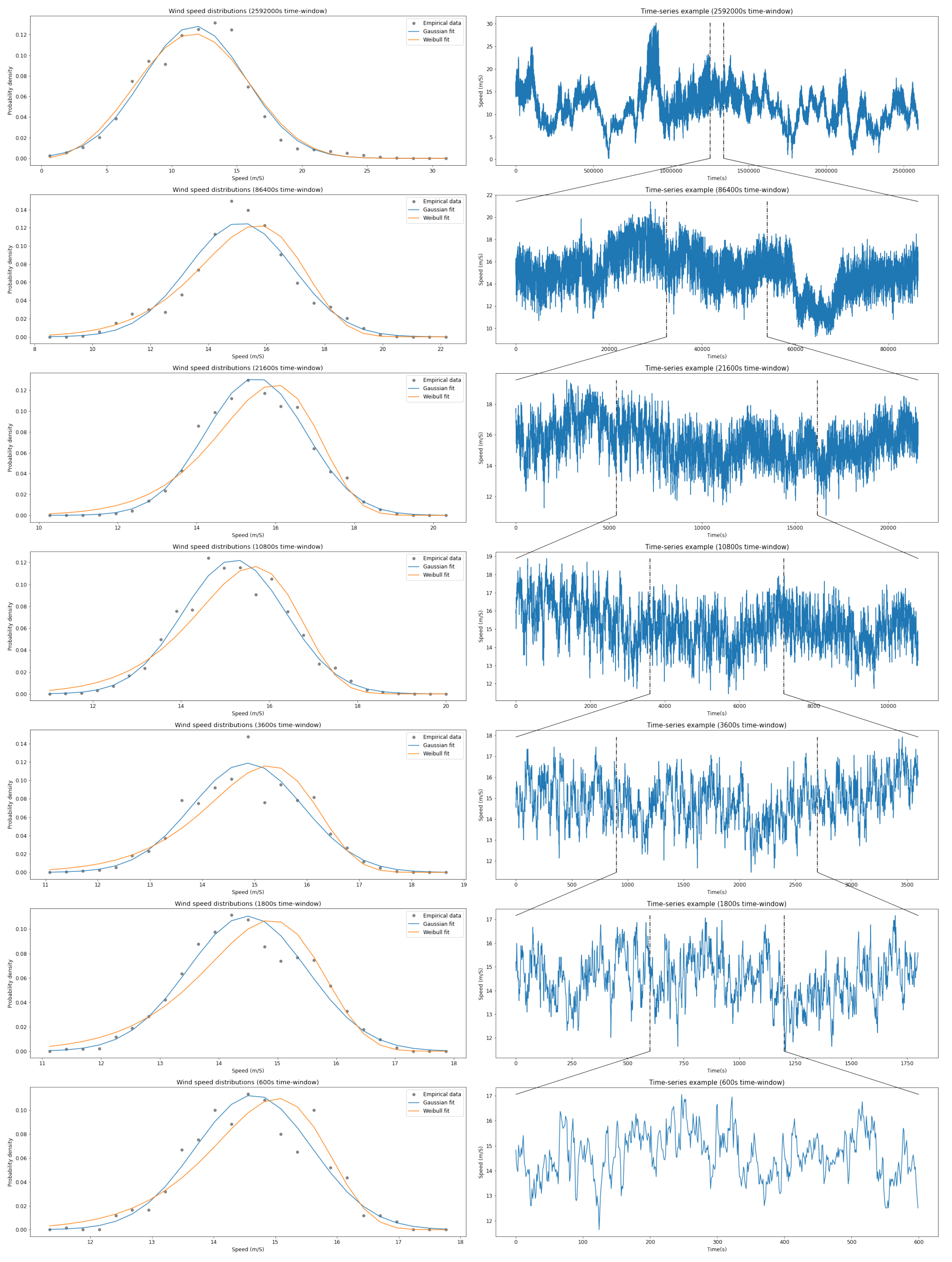
We detected that 1% of the total data points were NaNs (Not a Number). This fraction was discarded from the analysis. Furthermore, we analyze the data in different time-frames of length T, namely T = 10 , 30 , and 60 min and also 1 h, 3 h, 6 h, 1 day, and 1 month. We also discarded time windows with more than 40% of NaNs. Figure 2 illustrates both typical time series within this time-frame of length T (right), together with its wind-speed distribution (left). In the latter plots we also indicate the best Weibull and Gaussian distribution. It should be noted that, whereas for large time-frames, e.g., 1 month, the Weibull fits better than the Gaussian, for shorter time scales, of 10 min, Gaussian models seems to surpass Weibull. Below we address this point in more detail, after introducing our models and metrics.

2.2. The Weibull Distribution as a Model for Wind-Speed Measurements and Some of Its “Cousins”

The Weibull distribution is a common model for the distribution of measurements of wind speed v, defined as
f W ( v ) = k λ v λ k 1 exp v λ k ,
where λ and k are the scale and shape parameters, respectively. This was introduced by Waloddi Weibull in 1951 [29,30].
As shown in [31], a Weibull wind-speed distribution follows from a Gaussian distribution of each one of the velocity components in the two-dimensional plane, assuming that both components are completely uncorrelated and have zero mean and the same standard deviation, σ . For that particular case, the Weibull distribution yields k = 2 and λ = 2 σ . Indeed, as reported in the literature [32,33], when fitting wind-speed measurements with a Weibull distribution (1) the shape parameter k takes values typically around 2, and therefore such assumptions are acceptable.
Having introduced the Weibull distribution, we can now describe two of its “cousins”, namely, the Nakagami and the Rician distributions.
The Rician distribution [34] has a probability density function defined as
f R ( v ) = x σ R 2 exp v 2 + ν 2 2 σ R 2 I v ν σ R 2 ,
where I ( x ) represents the modified Bessel function of the first kind of x and σ and ν represent the spread parameter and the distance between the reference point and center of the distribution, respectively. Notice that, while the Bessel function is an odd function, I ( x ) = I ( x ) , here the argument x is always positive since σ , v , ν > 0 . For ν = 0 , the Rician distribution reduces to a Weibull distribution with k = 2 and λ = 2 σ R .
The Nakagami distribution is defined by [35]
f N ( v ) = 2 Γ ( m ) m Ω m v 2 m 1 exp m Ω v 2 ,
where Ω and m represent the spread and the shape parameters, respectively. For the particular case of m = 1 , the Nakagami distribution reduces to a Weibull distribution with λ = Ω and k = 2 / λ 2 . Since in the case of wind-speed measurements k 2 , we conclude that Nakagami distribution is a good model for wind-speed data series with a scale parameter of λ 1 .
Together with these two “cousin” distributions of the Weibull model, we also consider the usual Gaussian distribution, defined as
f G ( v ) = 1 σ 2 π exp 1 2 v μ σ 2 ,
where μ is the mean and σ is the standard deviation. As we will see, each one of these three variants is sometimes better than the Weibull distribution as a model for s.
Finally, for consistency, we will also consider other distributions, not usually assumed in wind-data modeling, namely the Gamma distribution, the inverse-Gamma distribution, and the log-normal distribution, none of which are reducible to a Weibull distribution. The Gamma distribution is defined by
f G ( v ) = 1 Γ k θ k v k 1 exp v θ ,
where θ and k are the scale and shape parameters, respectively. The inverse-Gamma distribution is defined by
f I ( v ) = β α Γ α v α 1 exp β v ,
where β and α are the shape and the scale parameters, respectively. The log-normal distribution is defined by:
f L ( v ) = 1 v σ 2 π exp ln v μ 2 2 σ 2 ,
where μ represents the mean and σ the standard deviation of the logarithm of the wind speed v.
Figure 3 illustrates each one of these distributions for two representative time windows, one with T = 10 min and another with T = 1 month. Note that the fit here is done by solving the parameter values of each distribution above to match the same mean and variance of the empirical wind-speed measurements in that window.

2.3. Performance Measures: Evaluating the Fitness of Each Model

We evaluate the performance of each model with respect to each of three questions:
(I)
How well does each model enable one to predict the next value of the wind speed?
(II)
How well does each distribution model fit the empirical histogram of measurements?
(III)
How well does each model enable one to predict the energy associated with the wind speed, i.e., the square of the wind speed?
To evaluate the prediction power of the next value of the wind speed, we define a quantity called Next-Point-Probability (NPP), defined as the probability of observing the empirical data point immediately following the time window where the probability distribution was calculated. When NPP is close to one, the predictive power is high, whereas a probability close to zero shows a low predictive power. For clarity, we consider henceforth the logarithm of the NPP, L = log ( N P P ) . It is important to note that this quantity serves the purpose of an out-of-sample metric of a distribution’s fit quality and also of a short-term propagator.
To fit each distribution to the empirical histogram of each time window, we consider the Kullback–Leibler divergence (KLD), which is a non-negative and non-commutative measurement, fulfilling a maximum likelihood estimation scheme [36]. It is also called Relative Entropy and is defined as
D K L ( f X | | ρ emp ) = i bins / data f X ( i ) log f X ( i ) ρ emp ( i ) ,
where ρ emp is the empirical distribution and f X is one of the models above. The sum runs over the number of bins for which the empirical histogram is defined or over the data points in each time window in case a kernel-based estimator is chosen, depending on how it is implemented. Empirical distributions with two local maxima were discarded, which represented less than 2 % of the total number of time windows. For the inverse-Gamma fits, infinite values could be obtained when the likelihood was lower than computational resolution, though this occurs for only 0.1 % of the total number of time windows, and therefore we discarded these windows for this model.
Finally, to estimate the prediction power of each model for predicting the energy from wind-speed data, we evaluated the square velocity relative deviation, namely
Δ = v emp 2 v fit 2 v emp 2 ,
where the average runs over the time window. Our own routine was implemented. It should be highlighted that the fitting was performed on the empirical measurements (not their square), and from that, v fit 2 was estimated. Empirical distributions with two local maxima were discarded, which cover 2 % of the total number of time windows.

3. Results: Turbulence Features, Wind-Speed Statistics, and Prediction of Speed and Energy

We present our results by showing first how the average speed and respective standard deviation change with the size T of the time windows. Those two quantities are shown in Figure 4a and Figure 4b, respectively. We observe an almost constant average speed, μ , together with a standard deviation, σ , which increases five times when increasing the size of the time windows from T = 10 min to T = 1 month. Consequently, the intermittency of wind-speed measurements, which is defined as the quotient between the standard deviation and the mean, namely I = σ μ , increases linearly with the standard deviations; see Figure 4c.
Since the intermittency increases monotonically with the time-window size T, one would expect that the fitness or prediction power, assessed with the metrics introduced above ( L , D K L , and Δ ), should decrease with T. However, as we will see next, this is not always the case.
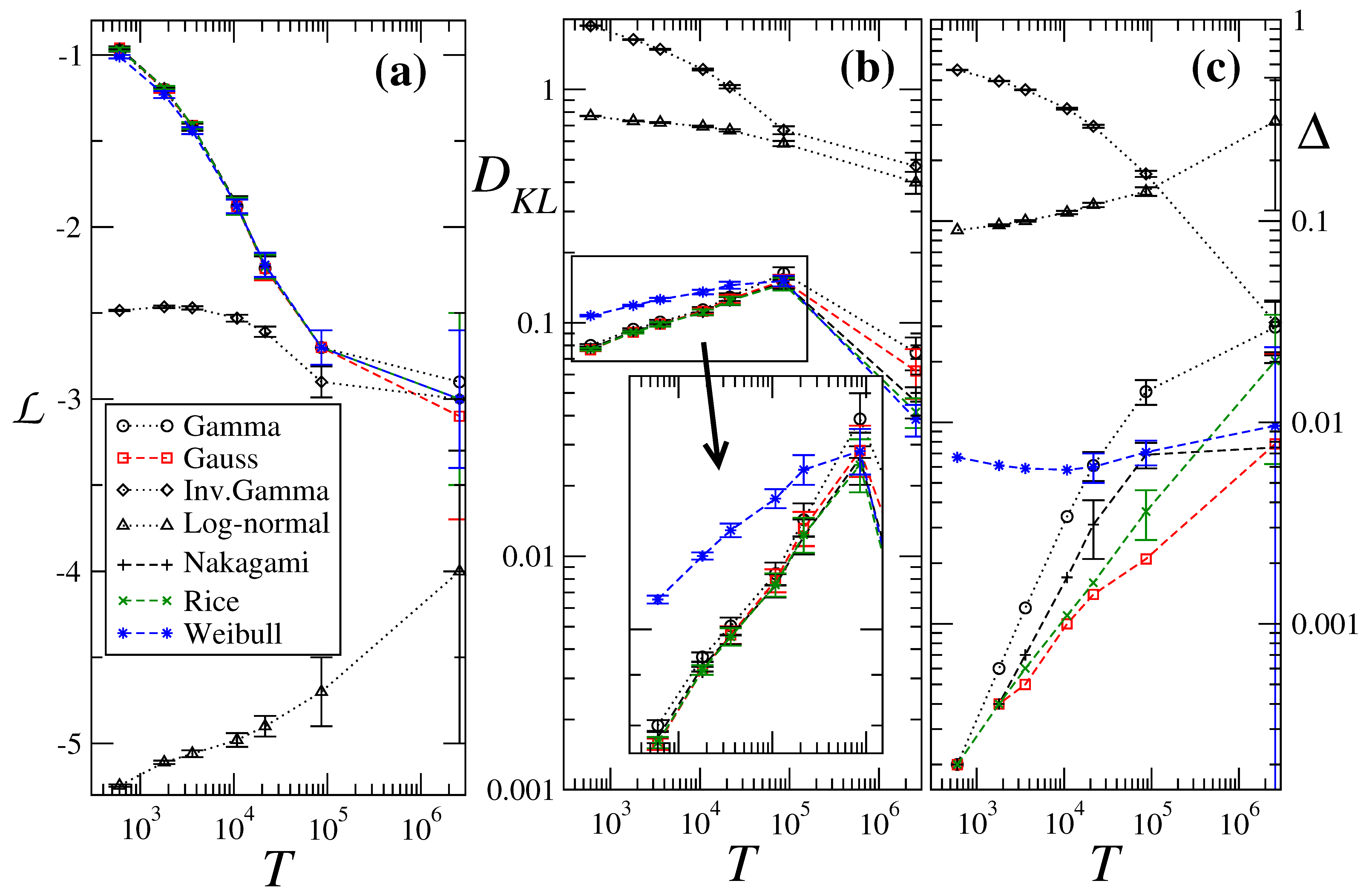
To address each one of the questions introduced above, in Section 2.3 we compute the respective metrics, namely L for question I, D K L for question II, and Δ for question III. The results are shown in Figure 5.
For the NPP, measured by L , the lower curves in Figure 5a are observed for the inverse-Gamma and log-normal. These two are therefore the worst models for next-point probability of the wind speed. As for all the other models, the performance in NPP is very similar and decreases monotonically with T. Interestingly, here the Gaussian model is ∼2% better than the Weibull one, being surpassed only by the Nakagami model, and sometimes the Rice model. Note that for windows of 1 month, all models perform equally well, with the exception of the log-normal model.
In Figure 5b we show how well the different distribution models fit the empirical wind-speed histogram, using D K L . Again, the log-normal and inverse-Gamma models perform poorly. Notably, for windows of 1 day or less, the Gauss, Gamma, Nakagami, and Rice distributions perform similarly, representing an improvement relative to the canonically used Weibull distribution (inset of Figure 5b).
When assessing the error in energy prediction, again we observe that the log-normal and inverse-Gamma distributions perform worse than the other distributions. We see that the Gauss, Gamma, Nakagami, and Rice distributions perform better than the Weibull here as well for smaller time windows. We observe in Figure 5c a performance of a few percent or less ( Δ 0.03 ) for all models, except log-normal and inverse-Gamma distribution, and for all window sizes T.
Finally, we assess the error in energy prediction. In Figure 5c, one observes a performance of a few percent or less, Δ 0.03 , for all models, except log-normal and inverse-Gamma distribution, and for all window sizes T. Here one observes that the Weibull model performs robustly, with an error of only Δ 0.01 . However, it does not surpass the performance of both Gauss and Nakagami. The Rice model is only worse than these latter three models for time windows of one month. Surprisingly, of all the models, the Gauss distribution model is the one retrieving the least amount of errors in energy predictions, independent of the window size. For better comparison, we provide in Table 1 all values of the curves plotted in Figure 5, for a better inspection of the values of all performance values.

4. Discussion and Conclusions

In this paper, we presented a systematic assessment of different distribution models for wind-speed measurements. The aim was to compare the performance of these models with the standard Weibull and Gauss distributions.
We provided quantitative evidence that, similarly to other studies, the Weibull distribution is not always the distribution that best fits wind speeds [4,5,6] and also not for predicting wind speeds and wind energy (square of the speed). For larger time-frames, namely within 1 day and 1 month, Weibull retrieves the best fit of the wind-speed distribution, supporting the standard assumption that—for large enough samples—wind-speed measurements follow a Weibull distribution.
However, we have provided evidence that, for all time windows, the Weibull model is not necessarily the best model for retrieving the prediction of the average wind speed and average wind energy. Moreover, while the Rice and Nakagami models, being related to the Weibull distribution, can retrieve more accurate predictions, it is surprising that Gauss performs equally well, and in some cases better than any other model.
Our findings may be of importance in the context of wind power forecasting and monitoring for power-grid assessment. Commonly, the Gauss model is used when addressing wind power and other observables in wind energy systems. Our results show that for 10-min or larger windows, Gauss models provide reasonable performance, and in some cases it is even the best model. However, one should note that, differently from what was shown in Figure 4, at time-scales smaller than minutes towards a few seconds or sub-seconds the intermittency may be higher than observed for 10-min windows.
For future research, one can consider studying the process in scale, seeing not only how standard deviation scales with the time-window scale, but also performing an analysis of correlations and Hurst exponents. Such analysis may shed further light on the limitations (or lack of them) of assigning a particular statistical distribution to wind speed.

Author Contributions

P.L. performed most of the simulations. A.Y. and P.G.L. contributed equally to the methodology design. P.G.L. contributed to conceptualization and overall supervision of the work. All authors have read and agreed to the published version of the manuscript.

Funding

This research received no external funding.

Data Availability Statement

Dataset available on request from the FINO.

Acknowledgments

The authors thank the FINO-project and the Forschungs- und Entwicklungszentrum Fachhochschule Kiel GmbH for providing the data sets. The authors also acknowledge Leonardo Rydin for useful discussions.

Conflicts of Interest

The authors declare no conflicts of interest.

References

  1. Tuller, S.E.; Brett, A.C. The characteristics of wind velocity that favor the fitting of a Weibull distribution in wind speed analysis. J. Appl. Meteorol. Climatol. 1984, 23, 124–134. [Google Scholar] [CrossRef]
  2. Jung, C.; Schindler, D. Global comparison of the goodness-of-fit of wind speed distributions. Energy Convers. Manag. 2017, 133, 216–234. [Google Scholar] [CrossRef]
  3. Jung, C.; Schindler, D. Wind speed distribution selection—A review of recent development and progress. Renew. Sustain. Energy Rev. 2019, 114, 109290. [Google Scholar] [CrossRef]
  4. Akgül, F.G.; Şenoğlu, B.; Arslan, T. An alternative distribution to Weibull for modeling the wind speed data: Inverse Weibull distribution. Energy Convers. Manag. 2016, 114, 234–240. [Google Scholar] [CrossRef]
  5. Ouahabi, M.H.; Benabdelouahab, F.; Khamlichi, A. Analyzing wind speed data and wind power density of Tetouan city in Morocco by adjustment to Weibull and Rayleigh distribution functions. Wind Eng. 2017, 41, 174–184. [Google Scholar] [CrossRef]
  6. Serban, A.; Paraschiv, L.S.; Paraschiv, S. Assessment of wind energy potential based on Weibull and Rayleigh distribution models. Energy Rep. 2020, 6, 250–267. [Google Scholar] [CrossRef]
  7. Rocha, P.; Raischel, F.; Boto, J.; Lind, P. Uncovering the evolution of non-stationary stochastic variables: The example of asset volume-price fluctuations. Phys. Rev. E 2016, 93, 052122. [Google Scholar] [CrossRef] [PubMed]
  8. Inglesi-Lotz, R.; Dogan, E. The role of renewable versus non-renewable energy to the level of CO2 emissions a panel analysis of sub-Saharan Africa’s Big 10 electricity generators. Renew. Energy 2018, 123, 36–43. [Google Scholar] [CrossRef]
  9. Furlan, C.; Mortarino, C. Forecasting the impact of renewable energies in competition with non-renewable sources. Renew. Sustain. Energy Rev. 2018, 81, 1879–1886. [Google Scholar] [CrossRef]
  10. Milan, P.; Wächter, M.; Peinke, J. Stochastic modeling and performance monitoring of wind farm power production. J. Renew. Sustain. Energy 2014, 6, 033119. [Google Scholar] [CrossRef]
  11. Milan, P.; Wächter, M.; Peinke, J. Turbulent Character of Wind Energy. Phys. Rev. Lett. 2013, 110, 138701. [Google Scholar] [CrossRef] [PubMed]
  12. Raischel, F.; Scholz, T.; Lopes, V.; Lind, P. Uncovering wind turbine properties through two-dimensional stochastic modeling of wind dynamics. Phys. Rev. E 2013, 88, 042146. [Google Scholar] [CrossRef]
  13. Hansen, K.; Mathiesen, B.V.; Skov, I.R. Full energy system transition towards 100% renewable energy in Germany in 2050. Renew. Sustain. Energy Rev. 2019, 102, 1–13. [Google Scholar] [CrossRef]
  14. Akermi, R.; Triki, A. The green energy transition and civil society in Tunisia: Actions, motivations and barriers. Energy Procedia 2017, 136, 79–84. [Google Scholar] [CrossRef]
  15. Zafar, U.; Rashid, T.U.; Khosa, A.A.; Khalil, M.S.; Rashid, M. An overview of implemented renewable energy policy of Pakistan. Renew. Sustain. Energy Rev. 2018, 82, 654–665. [Google Scholar] [CrossRef]
  16. Cadoret, I.; Padovano, F. The political drivers of renewable energies policies. Energy Econ. 2016, 56, 261–269. [Google Scholar] [CrossRef]
  17. Intergovernmental Panel on Climate Change. Technology-specific Cost and Performance Parameters. In Climate Change 2014: Mitigation of Climate Change: Working Group III Contribution to the IPCC Fifth Assessment Report; Cambridge University Press: Cambridge, UK, 2015; pp. 1329–1356. [Google Scholar] [CrossRef]
  18. Kampers, G.; Wächter, M.; Hölling, M.; Lind, P.G.; Queirós, S.M.; Peinke, J. Disentangling stochastic signals superposed on short localized oscillations. Phys. Lett. A 2020, 384, 126307. [Google Scholar] [CrossRef]
  19. Srinivasan, S.; Kumarasamy, S.; Andreadakis, Z.E.; Lind, P.G. Artificial Intelligence and Mathematical Models of Power Grids Driven by Renewable Energy Sources: A Survey. Energies 2023, 16, 5383. [Google Scholar] [CrossRef]
  20. Sim, S.K.; Maass, P.; Lind, P.G. Wind Speed Modeling by Nested ARIMA Processes. Energies 2019, 12, 69. [Google Scholar] [CrossRef]
  21. Friedrich, R.; Peinke, J. Description of a turbulent cascade by a Fokker-Planck equation. Phys. Rev. Lett. 1997, 78, 863–866. [Google Scholar] [CrossRef]
  22. Siegert, S.; Friedrich, R.; Peinke, J. Analysis of data sets of stochastic systems. Phys. Lett. A 1998, 243, 275–280. [Google Scholar] [CrossRef]
  23. Friedrich, R.; Peinke, J.; Sahimi, M.; Tabar, M. Approaching complexity by stochastic methods: From biological systems to turbulence. Phys. Rep. 2011, 506, 87–162. [Google Scholar] [CrossRef]
  24. Wächter, M.; Milan, P.; Mücke, T.; Peinke, J. Power performance of wind energy converters characterized as stochastic process: Applications of the Langevin power curve. Wind Energy 2011, 14, 711–717. [Google Scholar] [CrossRef]
  25. Anvari, M.; Lohmann, G.; Wächter, M.; Milan, P.; Lorenz, E.; Heinemann, D.; Kleinhans, D.; Rahimi Tabar, M.R. Short-term fluctuations of wind and solar power systems. New J. Phys. 2016, 18, 063027. [Google Scholar] [CrossRef]
  26. Lind, P.G.; Vera-Tudela, L.; Wächter, M.; Kühn, M.; Peinke, J. Normal Behaviour Models for Wind Turbine Vibrations: Comparison of Neural Networks and a Stochastic Approach. Energies 2017, 10, 1944. [Google Scholar] [CrossRef]
  27. Lind, P.G.; Wächter, M.; Peinke, J. Reconstructing the intermittent dynamics of the torque in wind turbines. J. Phys. Conf. Ser. 2014, 524, 012179. [Google Scholar] [CrossRef]
  28. Lind, P.G.; Herráez, I.; Wächter, M.; Peinke, J. Fatigue Loads Estimation Through a Simple Stochastic Model. Energies 2014, 7, 8279–8293. [Google Scholar] [CrossRef]
  29. Weibull, W. A Statistical Distribution Function of Wide Applicability. ASME J. Appl. Mech. 1951, 18, 293–297. [Google Scholar] [CrossRef]
  30. Abernethy, R. The New Weibull Handbook Fifth Edition, Reliability and Statistical Analysis for Predicting Life, Safety, Supportability, Risk, Cost and Warranty Claims, 5th ed.; Dr. Robert. Abernethy: Boston, MA, USA, 2006. [Google Scholar]
  31. Harris, R.; Cook, N. The parent wind speed distribution: Why Weibull? J. Wind Eng. Ind. Aerodyn. 2014, 131, 72–87. [Google Scholar] [CrossRef]
  32. Carrillo, C.; Cidrás, J.; Díaz-Dorado, E.; Obando-Montaño, A.F. An Approach to Determine the Weibull Parameters for Wind Energy Analysis: The Case of Galicia (Spain). Energies 2014, 7, 2676–2700. [Google Scholar] [CrossRef]
  33. Yu, J.; Fu, Y.; Yu, Y.; Wu, S.; Wu, Y.; You, M.; Guo, S.; Li, M. Assessment of Offshore Wind Characteristics and Wind Energy Potential in Bohai Bay, China. Energies 2019, 12, 2879. [Google Scholar] [CrossRef]
  34. Rice, S.O. Mathematical analysis of random noise. Bell Syst. Tech. J. 1944, 23, 282–332. [Google Scholar] [CrossRef]
  35. Nakagami, M. The m-distribution—A general formula of intensity distribution of rapid fading. In Statistical Methods in Radio Wave Propagation; Elsevier: Amsterdam, The Netherlands, 1960; pp. 3–36. [Google Scholar]
  36. Hershey, J.R.; Olsen, P.A. Approximating the Kullback Leibler Divergence between Gaussian Mixture Models. In Proceedings of the 2007 IEEE International Conference on Acoustics, Speech and Signal Processing—ICASSP ’07, Honolulu, HI, USA, 15–20 April 2007; Volume 4, pp. IV–317–IV–320. [Google Scholar]
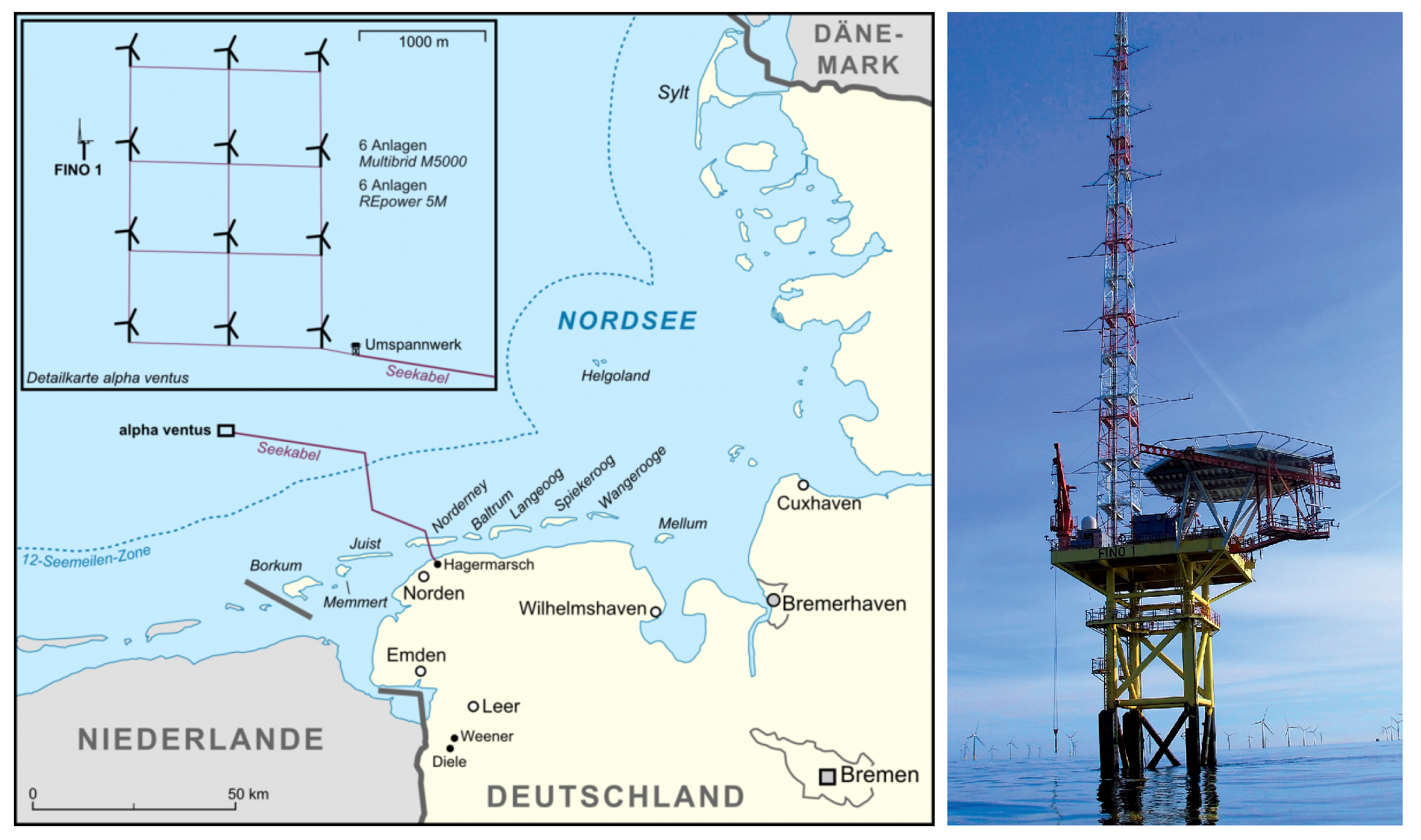
Figure 1. (Left) Location of the FINO-1 tower at the North Sea, as part of the Alpha Ventus wind park, and (Right) a close-up of the FINO-1 tower where the wind-speed measurements are collected at different heights. In this paper, we consider wind speed measured at 100 m with a sampling frequency of 1 Hz.
Energies 17 02621 g001
Figure 2. Wind speed measurements within time windows of different lengths, namely (from bottom to top), T = 600, 1800, 3600, 10,800, 21,600, 86,400, 2,592,000 s. On the right, representative time-series for each one of these time windows is shown, and on the left one sees the corresponding histogram of those wind-speed values (symbols), together with the best fit of a Weibull (orange, Equation (1)) and Gaussian (blue, Equation (4)) distribution. We use a Gaussian kernel for the density estimate.
Energies 17 02621 g002
Figure 3. Illustration of each one of the two-parameter distributions mentioned in Section 2.2 in two representative time windows for (Left) T = 600 s (10 min) and (Right) T = 2,592,000 s (1 month). As we will see, depending on the scale one considers (time-window size), the best model is different.
Energies 17 02621 g003
Figure 4. Assessing turbulence features within time windows of different sizes, T: (a) the mean μ of the wind speed, (b) the standard deviation, σ , of the wind speed, and (c) the turbulent intermittency, I = σ μ . While the mean of the wind speed is approximately independent of T, the standard deviation increases with the time-window size. Therefore, the intermittency of wind-speed fields seems to scale linearly with the standard deviation of wind speed (inset).
Energies 17 02621 g004
Figure 5. Assessing the fitness of different models of wind speed measured within a time window of size T. Here we consider three different types of fitness to evaluate the prediction power (see text): (a) How well each model is able to predict the next value of the wind speed, which is measured by the (logarithm of the) next-point-probability, L . (b) How well each distribution model fits the empirical histogram of measurements, which is measured by the Kullback–Leibler divergence, cf. Equation (8). (c) How well each model is able to predict the energy associated with the wind speed, i.e., the square of the wind speed, which is measured by the percentual deviation Δ , cf. Equation (9). Details on what the best models are can be found in the text.
Energies 17 02621 g005
Table 1. All values of the curves in Figure 5.
Time(s)GaussWeibullGammaInvGamNakagamiRiceLogN
6000.0770.1070.0801.8750.0780.0770.769
(±0.001)(±0.001)(±0.001)(±0.004)(±0.001)(±0.001)(±0.002)
18000.09100.1190.0941.6360.0920.0910.733
(±0.001)(±0.001)(±0.001)(±0.006)(±0.001)(±0.001)(±0.003)
36000.0990.1260.1011.4870.0990.0980.721
(±0.002)(±0.002)(±0.002)(±0.008)(±0.002)(±0.002)(±0.004)
D K L 10,8000.1120.1350.1141.220.1110.1110.694
(±0.003)(±0.003)(±0.003)(±0.01)(±0.003)(±0.003)(±0.006)
21,6000.1260.1450.1291.030.1240.1240.668
(±0.005)(±0.005)(±0.005)(±0.02)(±0.005)(±0.005)(±0.008)
86,4000.1510.1510.160.670.1490.1460.59
(±0.009)(±0.008)(±0.01)(±0.03)(±0.009)(±0.009)(±0.02)
2,592,0000.060.0390.070.470.0460.0410.40
(±0.015)(±0.006)(±0.01)(±0.07)(±0.007)(±0.006)(±0.04)
600−0.96−1.01−0.97−2.485−0.96−0.97−5.245
(±0.01)(±0.01)(±0.01)(±0.004)(±0.01)(±0.01)(±0.007)
1800−1.20−1.23−1.20−2.464−1.19−1.19−5.11
(±0.02)(±0.02)(±0.01)(±0.007)(± 0.01)(±0.01)(±0.01)
3600−1.41−1.44−1.42−2.47−1.41−1.41−5.06
(±0.02)(±0.02)(±0.02)(±0.01)(±0.02)(±0.02)(±0.02)
L 10,800−1.88−1.88−1.88−2.53−1.87−1.88−4.98
(±0.04)(±0.04)(±0.05)(±0.02)(±0.05)(±0.05)(±0.04)
21,600−2.24−2.22−2.24−2.61−2.23−2.23−4.90
(±0.07)(±0.07)(±0.07)(±0.03)(±0.06)(±0.07)(±0.06)
86,400−2.7−2.7−2.7−2.90−2.7−2.7−4.7
(±0.1)(±0.1)(±0.1)(±0.09)(±0.1)(±0.1)(±0.2)
2,592,000−3.1−3.0−2.9−3.0−3.0−3.0−4
(±0.6)(±0.4)(±0.4)(±0.4)(±0.5)(±0.5)(±1)
6000.00020.00670.00020.5630.00020.00020.0901
(±0.0001)(±0.0001)(±0.0001)(±0.001)(±0.0001)(±0.0001)(±0.0001)
18000.00040.00610.00060.4960.00040.00040.095
(±0.0001)(±0.0001)(±0.0001)(±0.001)(±0.0001)(±0.0001)(±0.001)
36000.00050.00590.00120.4490.00070.00060.100
(±0.0001)(±0.0001)(±0.0001)(±0.002)(±0.0001)(±0.0001)(±0.001)
Δ 10,8000.00100.00580.00340.3610.00170.00110.110
(±0.0001)(±0.0001)(±0.0001)(±0.004)(±0.0001)(±0.0001)(±0.002)
21,6000.00140.0060.0060.2960.0030.00160.120
(±0.0001)(±0.001)(±0.001)(±0.005)(±0.001)(±0.0001)(±0.003)
86,4000.00210.0070.0140.1720.0070.0040.140
(±0.0001)(±0.001)(±0.002)(±0.006)(±0.001)(±0.001)(±0.007)
2,592,0000.010.010.030.0310.010.020.3
(±0.01)(±0.01)(±0.01)(±0.009)(±0.01)(±0.01)(±0.2)
Disclaimer/Publisher’s Note: The statements, opinions and data contained in all publications are solely those of the individual author(s) and contributor(s) and not of MDPI and/or the editor(s). MDPI and/or the editor(s) disclaim responsibility for any injury to people or property resulting from any ideas, methods, instructions or products referred to in the content.