Article

Power System State Estimation Based on Fusion of PMU and SCADA Data

1
School of Electrical Engineering, Anhui Polytechnic University, Wuhu 241000, China
2
Key Laboratory of Advanced Perception and Intelligent Control of High-End Equipment, Chinese Ministry of Education, Wuhu 241000, China
*
Author to whom correspondence should be addressed.
Energies 2024, 17(11), 2609; https://doi.org/10.3390/en17112609
Submission received: 10 April 2024 / Revised: 23 May 2024 / Accepted: 25 May 2024 / Published: 28 May 2024

Abstract

:
This paper introduces a novel hybrid filtering algorithm that leverages the advantages of Phasor Measurement Units (PMU) to address state estimation challenges in power systems. The primary objective is to integrate the benefits of PMU measurements into the design of traditional power system dynamic estimators. It is noteworthy that PMUs and Supervisory Control and Data Acquisition (SCADA) systems typically operate at different sampling rates in power system estimation, necessitating synchronization during the filtering process. To address this issue, the paper employs a predictive interpolation method for SCADA measurements within the framework of the Extended Kalman Filter (EKF) algorithm. This approach achieves more accurate estimates, closer to real observation data, by averaging the KL distribution. The algorithm is particularly well-suited for state estimation tasks in power systems that combine traditional and PMU measurements. Extensive simulations were conducted on the IEEE-14 and IEEE-30 test systems, and the results demonstrate that the fused estimator outperforms individual estimators in terms of estimation accuracy.

1. Introduction

The estimation of a power system’s state constitutes a fundamental aspect of the energy management system within a power system dispatch center. This essential function involves the assessment of the current operational state of the power system based on diverse measurements and information [1,2]. The energy management system accomplishes the detection of erroneous data, maintenance of system stability, and enhancement of reliability by computing the phasors of each bus, encompassing both voltage magnitude and phase angle. Furthermore, within the power system context, a consistent and accurate state estimation is imperative for most Energy Management System (EMS) operations. Any significant faults or abrupt changes have the potential to induce severe issues in the power system, such as instability and blackouts [3].
Over the past few decades, there has been rapid advancement in SCADA systems, which have found extensive applications in the power industry. Virtually all EMSs worldwide have integrated SCADA [4]. A multitude of Remote Terminal Units (RTUs) deployed at remote locations collect local bus voltage, injected power, and current values, transmitting this data to the central terminal unit for consolidated state estimation. However, the measurements available in SCADA systems tend to exhibit relative slowness, and the physical distances within the power system are of significance. Additionally, SCADA systems are incapable of directly measuring power states.
With the widespread integration of Phasor Measurement Units (PMUs) and the support of existing dynamic state estimation tools, such as the Kalman filtering technique, there is now an enhanced capability to estimate the dynamic state of interconnected power systems with sufficient temporal precision. The PMU has a fast sampling frequency, delivering 30–60 measurement samples per second [5]. In contrast, conventional measurement systems within power systems, such as SCADA systems based on RTUs, offer a significantly lower rate of 1–2 measurement samples per second. With the acknowledgment of PMUs as a pivotal component of the future power grid, they are gradually replacing traditional SCADA systems [6]. Nevertheless, this transformation is unlikely to be accomplished in the short term. Despite certain advantages of PMUs over SCADA systems, a complete replacement of traditional SCADA systems in the short term poses a substantial challenge. The main obstacle to this challenge lies in the long-term dependence of most power systems on SCADA systems, with substantial investments made by enterprises in SCADA infrastructure [7,8,9]. Additionally, existing SCADA systems demonstrate stable operation within power systems, devoid of major issues or defects. Consequently, attempting a comprehensive replacement would result in severe operational losses. PMUs and traditional SCADA systems will coexist within the power grid [10,11,12]. This gives rise to an intricate scenario, necessitating the monitoring of system dynamics through a diverse array of sensors with varying sampling rates.
Opting for a strategy where PMUs are deployed at each bus, thereby simply measuring the power system’s state, would yield superior accuracy and speed compared to the conventional SCADA approach. Nevertheless, practical implementation constraints arise due to the high installation cost of PMUs, leading most power systems to deploy only a limited number of PMUs [13,14]. Nonetheless, the state of the power system can still be observed through the careful positioning of each PMU.
Hence, the amalgamation of measurement data from both SCADA and PMUs for hybrid power state estimation emerges as a more precise methodology [15,16]. This entails the strategic deployment of a limited number of PMUs to integrate observations from both PMUs and SCADA. Leveraging the expeditious measurement data from PMUs, this approach yields more accurate state estimates compared to reliance solely on traditional SCADA systems.
The majority of State Estimation (SE) methodologies identified in the literature that rely on SCADA–PMU measurements fall within the category of single SE. In this approach, PMU measurements are integrated with traditional SCADA measurements, forming what is termed HSE (Hybrid SE). The primary aim of this integration is to enhance precision without accounting for errors [17]. In the work documented in [18], the authors elucidate the formation of Jacobian matrices and covariance matrices encompassing both measurement types. The outcomes of testing demonstrate a substantial improvement in estimation precision. Another investigation, outlined in [18], analyzes two alternative approaches involving phasor current measurements, whether expressed in polar or rectangular coordinates. A notable limitation across these approaches is the neglect of sampling rate differences between PMU and SCADA measurements, essentially executing state estimation on the slower time scale of SCADA. However, to capture the real-time state of the power system, estimation must be conducted at an appropriate fine time scale.
In response to the aforementioned issues, this paper proposes a hybrid state estimation strategy based on EKF. The strategy involves predicting the current SCADA estimate using the EKF algorithm to establish a new estimate. The measurement time scale of this new estimate aligns with that of PMUs, allowing for the fusion of the PMU estimate and the newly defined estimate. The introduced fusion estimator effectively addresses the disparate sampling rates between PMUs and SCADA. In comparison to [19], our newly defined estimate is obtained using the EKF algorithm under KLA averaging, resulting in a new estimate that is closer to the actual SCADA measurements.
The rest of this paper is structured as follows: Section 2 introduces the conventional power system model, and Section 3 derives the KLA formula and utilizes it to establish a new state estimation through EKF. The filtering steps of EKF are demonstrated in Section 4, followed by an introduction to the working principles of fusion algorithms, explaining how to incorporate new estimates into the fusion estimator. Section 5 presents the results of simulation experiments, demonstrating the significant advantages of the fusion estimator. Finally, in Section 6, a summary and outlook on this paper’s work are provided.

2. The Model of the Power System

2.1. Power System Dynamical Equations

The estimation of the power system state is a critical component in the EMS at the power system dispatch center, functioning as a key element. This process primarily aims to determine the current operational state of the power system by utilizing various measurement data collected from its components [20]. In this study, we assume that the measurement values and state variables of the power system are denoted by m and n, respectively. Typically, in power information systems, there exists a complex nonlinear relationship between the measurement values and state variables within the system [21]:
z = h ( x ) + v
z 1 z 2 z m = h 1 ( x 1 , x 2 x n ) h 2 ( x 1 , x 2 x n ) h m ( x 1 , x 2 x n ) + v 1 v 2 v m
where v is the measurement error vector in R m × 1 . The mean of R is zero, and it follows a normal distribution with R = diag ( σ 1 2 , , σ m 2 ) . z R m × 1 is the measurement vector and  x R n × 1 represents the state variables to be estimated. The function h ( · ) describes the relationship between z and x . z is the measurement vector and  x is the state vector. The nonlinear relationship between z and x is given as follows [22]:
P i = V i j Ω i V j ( G i j cos θ i j + B i j sin θ i j )
Q i = V i j Ω i V j ( G i j sin θ i j B i j cos θ i j )
P i j = V i 2 ( g s i + g i j ) V i V j ( g i j cos θ i j + b i j sin θ i j )
Q i j = V i 2 ( b s i + b i j ) V i V j ( g i j sin θ i j + b i j cos θ i j )
where V i stands for the voltage at bus i; P i is the active power injections at bus i; P i j represents the real power flows from bus i to bus j; Q i denotes the active and reactive power injections at bus i; Q i j represents reactive power flows from bus i to bus j; θ i indicates the phase angle at bus i, and  θ i j is the phase angle difference between buses i and j. The line admittance between buses i and j is given by G i j + j B i j , and the admittance of the shunt branches at bus i is represented by g i j + j b i j . Finally, Ω i is the set of buses connected to bus i.

2.2. Measurement Equation

As mentioned in Section 1, the sampling rate of a PMU is several times that of SCADA. However, when applying standard Kalman filtering, it is necessary to have two sets of measurements obtained at the same sampling rate. Therefore, we make the following assumptions:
Assumption A1.
The ratio of the sampling rates of the two types of sensors is a positive integer: where n p and n s are the sampling rates of the PMU and SCADA, respectively, and the measurement instant of the two samples is represented by k p and k s , respectively, and R is the ratio of the sampling rates of the two, i.e., the r-th SCADA measurement timestamps coincides with the ( r × n )-th measurement timestamps.
In this article, it is assumed that the sampling rate ratio of PMU to SCADA is 4:1, i.e.,  r = 4 . As shown in Figure 1, it can be observed that during the initial measurement phase ( k = 0 ), PMU and SCADA measurements coincide instantaneously. Subsequently, the PMU measures every four times, while SCADA measures only once. Moreover, whenever the measurements of the two coincide, it is always the case that k s = n and k p = r × n .

2.2.1. PMU Measurements

Assuming PMUs are deployed within a subset of the bus, denoted as subset B i , where i ranges from 1 to N, N denotes the total number of buses, the measurement vector of PMUs in this paper comprises the voltage magnitude and phase angle of bus nodes. Consequently, we can derive the following measurement equations.
z p = h p ( x p ) + v p
where z p is the vector of measured values obtained from the PMU, z p R m p , and it is essential that the quantity of measurements exceeds the count of the state variable, i.e.,  m p = 2 n p + 1 . x p denotes a vector of state variables, where each element corresponds to the voltage magnitude and phase angle of the bus node.

2.2.2. SCADA Measurements

The measurements of SCADA are received at a rate of n s . Here, the measurement vectors of SCADA are the line power P i j and Q i j . Similar to the measurement equations of PMUs above, the measurement equations of SCADA can be obtained as follows:
z s = h s ( x s ) + v s
where z s R m s , as we know from Section 2.2.1, m s = 2 n s + 1 . v s is the measurement noise, It is worth noting that the measurement noise in Equation (7) shares the same characteristics as v s , both being Gaussian white noise.
It is important to note that this discretization does not impact the measurement Jacobian matrix H . As mentioned earlier, we use the SCADA system to monitor active power and reactive power, and then transfer the collected active power and reactive power data to the RTU. Simultaneously, the PMU system collects voltage amplitude and phase angle data.
In fact, it is possible to combine active power and reactive power into a complex power, which can then indirectly allow SCADA to measure voltage amplitude and phase angle, as follows:
S = P i j + j Q i j
where S represents complex power and j denotes the imaginary unit. We can then use the following complex current formula to combine the magnitude and phase angle of the currents into one complex current,
I c = I e j θ
where θ is the phase angle of the current. Using the complex power formula, we can link complex power with complex current,
S = V b I c
so
V b = P i j + j Q i j I e j θ
As a result, we can obtain the magnitude and phase angle of the voltage, making it convenient for us to perform data fusion.

3. Dynamic State Estimation Model

The state variables of the power system generally exhibit a multidimensional nonlinearity, a property that is typically reflected in the power flow equations within the power system. In dynamic state estimation, its state equation and measurement equation can be described by the following Equations [22]:
x k + 1 = f ( x k ) + w k
z k = z ( x k ) + v k
where f is the state transition equation from state vector x k to x k + 1 ; x k indicates the state vectors at time k, and for the same reason, x k + 1 denotes the state vectors at time k + 1 , respectively. h signifies the nonlinear connection between x and z . w k and v k denote the systematic error and measurement error at time k, assuming w k and v k are uncorrelated and follow white Gaussian noise distributions with zero mean. Then, we will denote their error covariance matrices by Q and R , respectively; z k is the measurement vector at time k.
The Kalman filter, as a linear estimator, finds extensive application [23]. However, in power information physical systems, the power system equations exhibit highly multi-dimensional and nonlinear characteristics, rendering the direct use of the standard Kalman filter impractical. Therefore, in this study, we instead contemplate utilizing the EKF for state estimation. The linearization model of the EKF can be described by the following Equations:
x k + 1 = F k x k + G k + v k
z k = H k x k + v k
where F k = f f x | x = x ^ k x | x = x ^ k is a non-zero diagonal matrix that signifies the relationships among state variables. G k is the input matrix.

3.1. PMU-Only State Estimation

According to the measurement equation in Section 2, we can obtain the measurement values based on the PMU time scale n p . The state estimation equation at point k p is:
x ^ p ( k p + 1 | k p + 1 ) = E { x p ( k p + 1 ) | z p ( 1 ) , z p ( 2 ) , , z p ( k p + 1 ) }
where x ^ p is the estimation of x p ( k p + 1 ) based on the measurement values obtained from PMU observations up to time k p + 1 , k p is the instant of PMU measurement within the time interval T, and z p ( 1 ) , z p ( 2 ) , , z p ( k p + 1 ) refers to the measurement values taken by the PMU at various instants from time 1 to k p .

3.2. SCADA-Only State Estimation

Similar to the derivation process in Equation (17), we can obtain the measurement values based on the SCADA time scale n s . The state estimation equation at point k s is:
x ^ s ( k s + 1 | k s + 1 ) = E { x s ( k s + 1 ) | z s ( 1 ) , z s ( 2 ) , , z s ( k s + 1 ) }
where x ^ s is the estimation of x s ( k s + 1 ) based on the measurement values obtained from SCADA observations up to time k s + 1 , k s is the instant of SCADA measurement within the time interval T, and z s ( 1 ) , z s ( 2 ) , , z s ( k s + 1 ) refers to the measurement values taken by SCADA at various instants from time 1 to k s .

3.3. The SCADA State Estimation at Scale n p

According to different time steps, there are differences in the measurement equations of PMUs and SCADA, so for the fusion of PMUs and SCADA, we can see it as a special case of multi-scale multi-sensor fusion algorithms [24,25]. As shown in Figure 2, we use the process of working to establish a new estimation x ^ s based on the measurements of SCADA, and the new estimation is carried out on the estimation results of SCADA in the time scale of the PMU. The new estimation is made on the time scale of the PMU to the measurements of SCADA, and the KLA averaging algorithm is used to generalize the noise distribution of the original state estimation of SCADA to comply with the closest distribution as our new estimation; the specific process is as follows:
From Section 2, we find that v p , v s are Gaussian white noise, so their probability density functions all obey a Gaussian distribution, hence we defined a community as,
q i = { p p 1 , p p 2 , p p m , p s 1 , p s 2 , p s w }
where { p p 1 , p p 2 , p p m } is the PDF of PMU process noise, and { p s 1 , p s 2 , p s w } is the PDF of SCADA process noise
Now, we find a distribution P that is close to q i ; here, we use the Kullback–Leibler average (KLA) of N PDFs q i ( · ) belonging to the parametric family P is the PDF defined as follows,
p ¯ = arg inf p P i = 1 N 1 N D K L p q i
According to the definition of KL dispersion, we can obtain
D K L = i = 1 N p ( x ) log p ( x ) q i ( x )
Now, we simplify (20) to obtain:
D K L = i = 1 N p ( x ) log p ( x ) q i ( x ) = i = 1 N p ( x ) log p ( x ) p ( x ) log q i ( x ) = i = 1 N p ( x ) log p ( x ) i = 1 N p ( x ) log q i ( x ) = p ( x ) N log p ( x ) log i = 1 N q i ( x ) = p ( x ) log p ( x ) N i = 1 N q i ( x )
In Equation (19), inf in mathematics denotes the lower exact bound, i.e., the smallest upper bound in a set of real numbers. According to the definition of KL scatter, KL scatter is greater than or equal to zero. Therefore, if we take the smallest lower bound, we can obtain the following equation:
p ( x ) N = i = 1 N q i ( x )
In Section 2, we can see that v p and v s are both Gaussian white noise, so their probability density functions (PDF) both obey a Gaussian distribution. The vector form of a Gaussian distribution usually refers to the vector form of a multivariate Gaussian distribution Suppose that x = x 1 , x 2 , , x n T is an n-dimensional vector whose multivariate Gaussian distribution has a probability density function of
p ( x ) = 1 ( 2 π ) n 2 | Σ | exp 1 2 ( x μ ) T Σ 1 ( x μ )
where μ is a k -dimensional vector called the mean vector and Σ is the noise covariance of k × k . k is the dimension of the random vector x . In addition, there is another representation of the PDF in Gaussian format, which is represented in the canonical form of
p ( x ) = exp ζ + η T x 1 2 x T Λ x
where Λ = Σ 1 , η = Σ 1 μ and ζ = 1 2 d log 2 π log | Λ | + η T Λ 1 η ; so, we first start analyzing the product of N identical PDFs,
p ( x ) N = exp i = 1 N ζ + η T x 1 2 x T Λ x = exp N ζ + ( N η ) T x 1 2 x T N Λ x
Now, the product of N Gaussian PDFs i = 1 n is
i = 1 n q i ( x ) = exp ζ i = 1 n + i = 1 N η i T x 1 2 x T i = 1 N Λ i x
where
ζ i = 1 N = i = 1 N ζ i = 1 2 n d log 2 π i = 1 N log Λ i + i = 1 N η i T Λ i 1 η i
So
i = 1 N q i ( x ) = exp ζ i = 1 N + ζ N ζ N + i = 1 N η i T x 1 2 x T i = 1 N Λ i x = exp ζ i = 1 N ζ N exp ζ N + η N T x 1 2 x T Λ N x
where
Λ N = i = 1 N Λ i , η N = i = 1 N η i
and
ζ n = 1 2 N d log 2 π log Λ N + η N T Λ N 1 η N
So
i = 1 N q i ( x ) = exp ζ N + η N x 1 2 x T Λ N x
Comparing this with the previous equations, we can see that for Equation (22) to hold, the coefficients in Equations (24) and (27) need to be equal, so
N Λ = Λ N N η = η N
Substituting the data in the standard form of Gaussian PDFs, we obtain
Σ ¯ 1 = 1 N i = 1 N Σ i 1 μ ¯ Σ ¯ 1 = 1 N i = 1 N Σ i 1 μ i
where Σ ¯ and μ ¯ will be considered as the measurement noise for the new estimation. From Equation (28), we can see that the covariance matrix of the new distribution P is smaller than the covariance matrix of the individual probability density functions. If v f , is the noise of the fused estimating equations, we can obtain the following state estimating equations,
z s p = h s ( x s p ) + v s p
where z s p is the newly established estimated measurement equation, x s p is the state vector of the SCADA measurement equation, and  v s p is the noise vector obtained by KLA, which approximates the noise distributions of SCADA and the PMU, with a mean of μ ¯ and a variance of Σ ¯ .
From Equation (28), it is not difficult to see that the noise adopted by the measurement equation established in this article should be situated between v p and v s , and it is closer to v p . Compared to traditional SCADA measurement equations, Equation (29) combines the noise characteristics of the two sets of traditional measurement equations more effectively, making it more suitable as a measurement equation in the fusion process.
Because of the complexity and multi-dimensionality of the power system, along with the variability of loads in the network, it is challenging to determine the state transition matrices in the EKF. The use of linearized state equations introduces errors. Therefore, this paper employs the Double Exponential Smoothing method to forecast the state values at the following time point. In the Kalman initial value prediction, the exponential smoothing method omits the step of estimating the initial state, and through the weighted average of the observed data, the initial state estimation can be determined quickly, and through this weighted average, quickly makes the prediction value close to the real value to accelerate the convergence of the filter, saving calculation time and reducing the complexity of the calculation. Its state equations can be expressed as follows:
x ^ k + 1 | k = a k + b k a k = τ x ^ k + ( 1 λ ) x ^ k | k 1 b k = λ ( a k a k 1 ) + ( 1 λ ) b k 1
where x ^ k p is the state estimation vector and x ^ k p | k p 1 represents the predicted vector at time k p , respectively; and τ and λ are both indicated as smoothing factors. After calculation, we choose τ = 0.84 and λ = 0.06 . Hence, the linearized state equation can be expressed as,
x ^ k + 1 | k = τ ( 1 + λ ) x ^ k + ( 1 + λ ) ( 1 + τ ) x ^ k | k 1 λ a k 1 + ( 1 τ ) b k 1

4. Data Fusion

4.1. Filter Step

The collective system equations are summarized below.
x k + 1 = f ( x k , μ k ) + w k
z p = h p ( x ) + v p
z s = h s ( x ) + v s
z s p = h s ( x ) + v s p
Here, we are using an extended Kalman filter for state estimation of PMU and SCADA monitoring data. The specific prediction and updating steps of the extended Kalman filter algorithm are as follows:
(1) Forecasting steps:
x ^ s | s 1 = F s 1 x ^ s 1
P s | s 1 = F k 1 F k 1 F k 1 T + Q k 1
(2) Updating steps:
x ^ s = x ^ s | s 1 + K s [ z s h ( x ^ s | s 1 ) ]
K s = P s | s 1 H s T ( H s P s | s 1 H s T + R s ) 1
P s = ( I K s H s ) P s | s 1
where P k | k 1 and P k represent the covariance matrices of the prior and posterior estimation errors at time k, respectively, while K k stands for the Kalman gain at time k. The initial state value is set as P 0 = 0 , and the estimation error matrix P 0 is derived using exponential smoothing, as described in Equations (29) and (30).
(1) Forecasting steps:
x ^ p | p 1 = F p 1 x ^ p 1
P p | p 1 = F k 1 F k 1 F k 1 T + Q k 1
(2) Updating steps:
x ^ p = x ^ p | p 1 + K p [ z p h ( x ^ p | p 1 ) ]
K p = P p | p 1 H p T ( H p P p | p 1 H p T + R p ) 1
P p = ( I K p H p ) P p | p 1

4.2. PMU Observability Issues

Both SCADA observability and PMU observability are essential prerequisites for implementing the estimation fusion strategy. These conditions are crucial for computing individual estimates, denoted as x ^ s p and B , which are subsequently fused. The assumption of network observability based on SCADA measurements is practical, as current SCADA-based state estimation techniques utilize metering schemes designed to ensure observability even under challenging conditions. However, the situation is different for PMU observability due to the limited penetration of PMUs in power networks, with no significant changes expected in the short term.
For the problem of PMU observability, ref. [26] proposes to assign a priori information for PMU unobservable buses as pseudo-measurement data. This method solves the problem of PMU global observability in the fusion process but increases the computational volume in the fusion process. To better solve this problem, this paper adopts the method of assigning the PMU positions through careful deployment, which both maximizes limiting the number of PMUs to reduce the cost and makes the PMUs globally observable during the fusion estimation process.
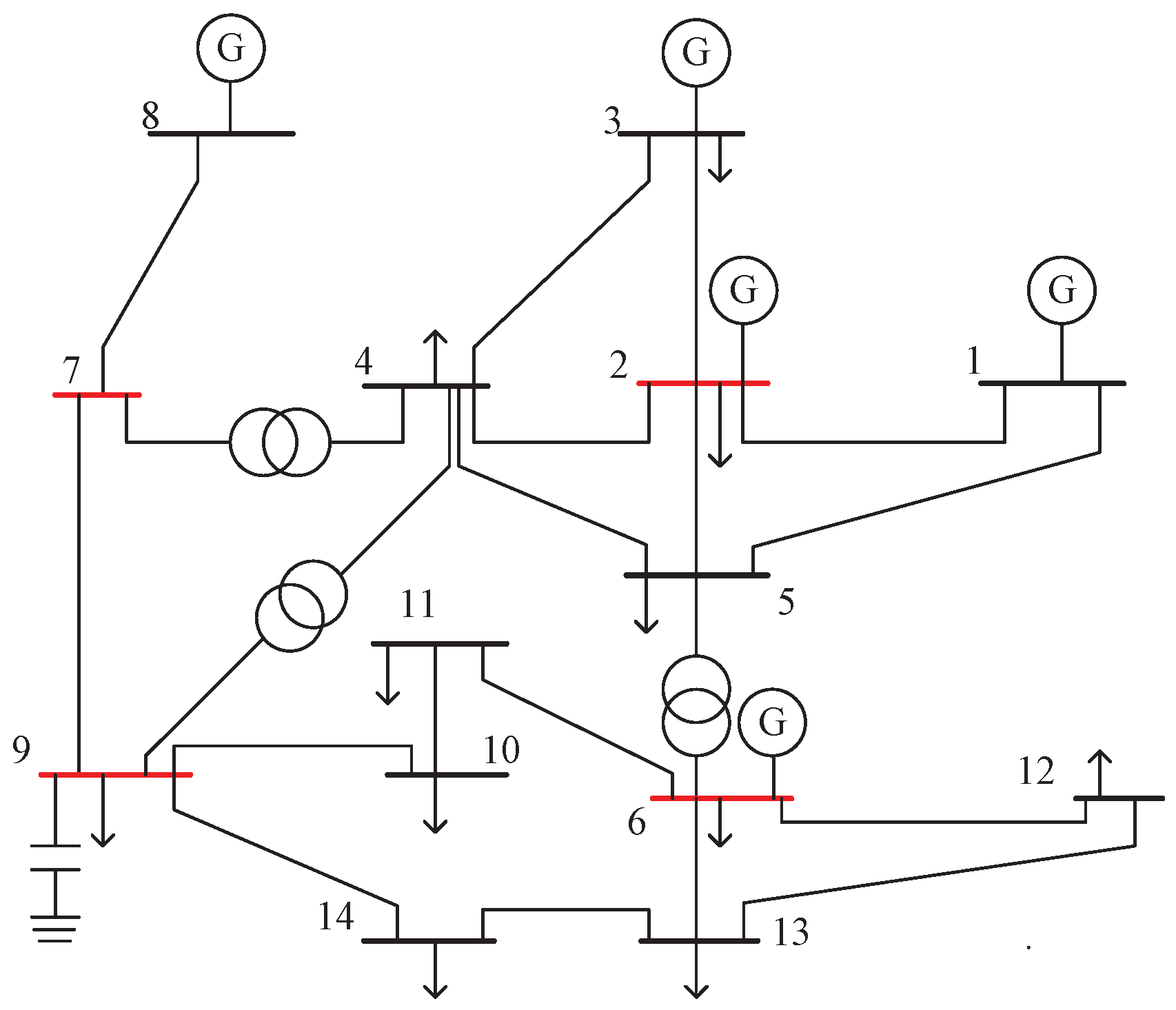
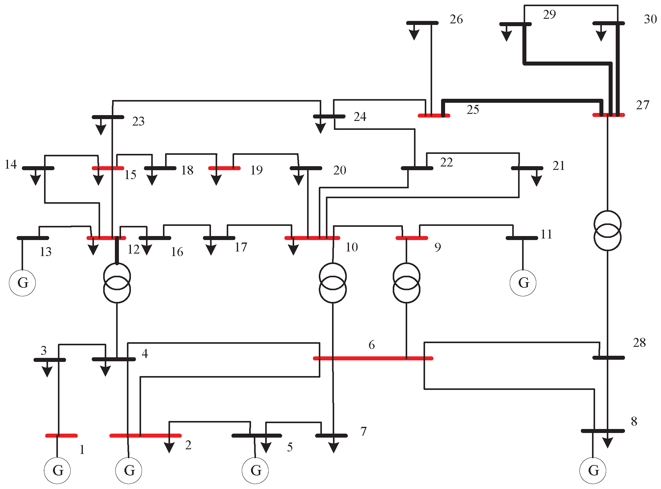
In accordance with the optimal PMU placement outlined in refs. [27,28,29,30]. As shown in Figure 3, in the IEEE-14 system, PMUs are placed at the optimal placement points of nodes 2, 6, 7, and 9. Meanwhile, nodes 1, 2, 6, 9, 10, 12, 15, 19, 25, and 27 are the optimal locations of PMUs in the IEEE-30 bus system. This is shown in Figure 4. It is worth noting that in Figure 3 and Figure 4, we have labeled buses deployed with PMUs in red, while the others are indicated in black. This placement strategy achieves global observability of the system with the minimum number of PMUs while also possessing higher redundancy compared to other strategies in terms of information redundancy.

4.3. Bar-Shalom–Campo Data Fusion

Now, we define the fusion-based estimation as follows,
x ^ f ( k p + 1 | k p + 1 ) : = E x p ( k p + 1 ) z s p ( 1 ) , z s p ( 2 ) , , z s p ( k p + 1 ) z p ( 1 ) , z p ( 2 ) , , z p ( k p + 1 )
where x ^ f represents the fused state estimate. This formula describes the predicted value of the state variable x ^ f at time step k p + 1 , given that the prediction is based on two sets of previously collected measurement data: z s p ( 1 ) , z s p ( 2 ) , , z s p ( k p + 1 ) and z p ( 1 ) , z p ( 2 ) , , z p ( k p + 1 ) . The expectation operation E { · } computes a weighted average over all possible values of the state variable x p ( k p + 1 ) given these two sets of measurement data.
The fuse state estimate, denoted as x ^ f , in the context of fusion, can be mathematically formulated as a weighted combination of the individual sensor-based estimates. This is expressed by Equation [12]:
x ^ f = i = 1 N w i x i
where x i represents the estimate obtained from the i-th sensor, and w i denotes the corresponding weight assigned to the estimate of that sensor. This approach leverages the collective information from multiple sensors to enhance the accuracy and robustness of the overall state estimation process.
This paper particularly focuses on the scenario where the consideration is limited to two categories of sensors. For this, assuming that w 1 and w 2 are uncorrelated, Equation (37) can be rewritten as [31,32]:
x ^ f = w 1 x ^ s p + w 2 x ^ p
where w 1 and w 2 are weighting matrices satisfying w 1 + w 2 = I , and I is the Identity Matrix.
The determination of weighting matrices can be achieved through the resolution of the subsequent optimization problem:
min w 1 , w 2 E { ( x ^ f x p ) ( x ^ f x p ) T }
The solution to the aforementioned constrained problem can be derived from the Bar-Shalom–Campo fusion formula:
w 1 = P s p 1 P s p 1 + P p 1 w 2 = P p 1 P s p 1 + P p 1
where P s p and P p are the estimation error covariance matrices of x ^ s p and x ^ s p , respectively. Similarly, according to the Bar-Shalom–Campo formula, we can obtain the error covariance matrix P f of the fused,
P f = P s p + P p P s p · P p 1
Based on the above, the PMU and SCADA data fusion method proposed in this paper is shown in Algorithm 1.
Algorithm 1 Multi-sensor multi-rate fusion method
Input: Sampling period n p , n s ; measurement value v p , v s ; initial state x ^ 0 and state error covariance P 0 ; noise covariance matrix R p , R s ; smoothing factor a , b .
Output: integrated estimation result x ^ f ;
1:
Extract measurement vector z p , z s ,calculate Jacobian matrices separately H p , H s ;
2:
Using exponential smoothing to forecast state variables, serving as the initial state vector.
3:
for all  k = 1 : N 1  do
4:
   Compute the measurement noise v s p of z s p using the KLA algorithm (Equations (18)–(28));
5:
   if  k > 1   then
6:
     if  r e m ( k , n s ) = = 0  then
7:
       Perform predictive updating on x ^ p ( 0 ) using Equations (27) and (28);
8:
        x ^ f ( 1 ) = x ^ p ( k + 1 ) ;
9:
     else
10:
       Obtain the initial state variable x ^ s p ( 0 ) using exponential smoothing;
11:
       Perform predictive updating on x ^ s p ( 0 ) using Equations (29)–(31);
12:
       Calculate weight matrices w 1 , w 2 ;
13:
        x ^ f ( k + 1 ) = w 1 x ^ p ( k ) + w 2 x ^ s ( k + 1 ) ;
14:
     end if
15:
   else if  k > 1  then
16:
     Perform predictive updating on x ^ p ( 0 ) using Equations (27) and (28);
17:
      x ^ f ( 1 ) = x ^ p ( k + 1 ) ;
18:
   end if
19:
end for

5. Simulation Result

This study utilized MATLAB R2018b for simulation purposes. To obtain the measurement data, this study employs the MatPower 7.1 toolbox in MATLAB to perform Gauss–Newton load flow calculations [33,34], which are used to update the voltage magnitudes across the entire system. The outcomes of the load flow calculations, particularly the voltage magnitudes and phase angles, depict the genuine state variables of the system. In addition, to observe the state over a long period, the total simulation time T is set to 80 s. According to Assumption 1 in Section 2.2, within T = 80 s, the measurement data from the PMUs should be four times that of SCADA. Therefore, in the simulation, the sampling time for the PMUs is set to 25 ms, and for SCADA, it is set to 1 s. Table 1 shows the measurement data of the PMU we used. Furthermore, to more closely simulate real-world operating conditions, Gaussian noise with a mean of zero is added to the observation data from both the PMU and SCADA, where σ s = 0.002 and σ p = 0.001 .
In order to enhance the accuracy of the simulation experiments, this simulation will be conducted separately on the IEEE-14 and IEEE-30 bus systems. Due to the significantly higher accuracy of PMUs compared to SCADA, and the large discrepancies observed between SCADA and PMU results in simulation output, the simulation does not directly depict SCADA simulation results in the graphical representation. Instead, it presents the estimation errors between SCADA and the PMUs in tabular form, as shown in Table 2, to visually illustrate the performance gap between PMUs and the fusion estimator. If the estimation error of SCADA is greater than that of the PMUs, and the performance after fusion is superior to that of the PMUs alone, it is sufficient to demonstrate that the fusion estimator outperforms individual estimators.

5.1. Comparison of State Values between Single Estimator and Fusion Estimator

In the power system, voltage magnitude and angle are important parameters describing the state of the power system. Through the estimation of the state of voltage magnitude and angle of the power system, this approach can discover and deal with the abnormal situation in the power system in time, and improve the stability and reliability of the power system. Secondly, it can be used for fault diagnosis and fault location of the power system. Through the estimation of voltage magnitude and angle state of the power system, the type and location of faults in the power system can be judged, providing guidance for fault handling. Therefore, in this simulation experiment, we focus on observing the estimation results of the estimator for voltage magnitude.
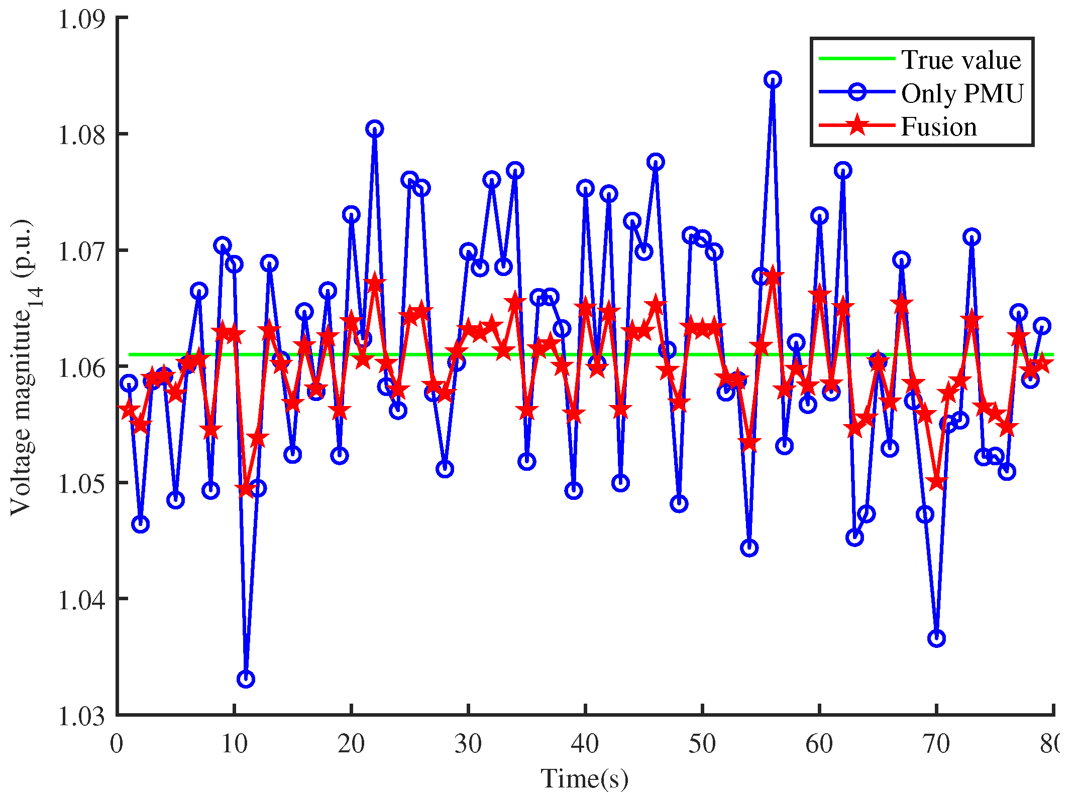
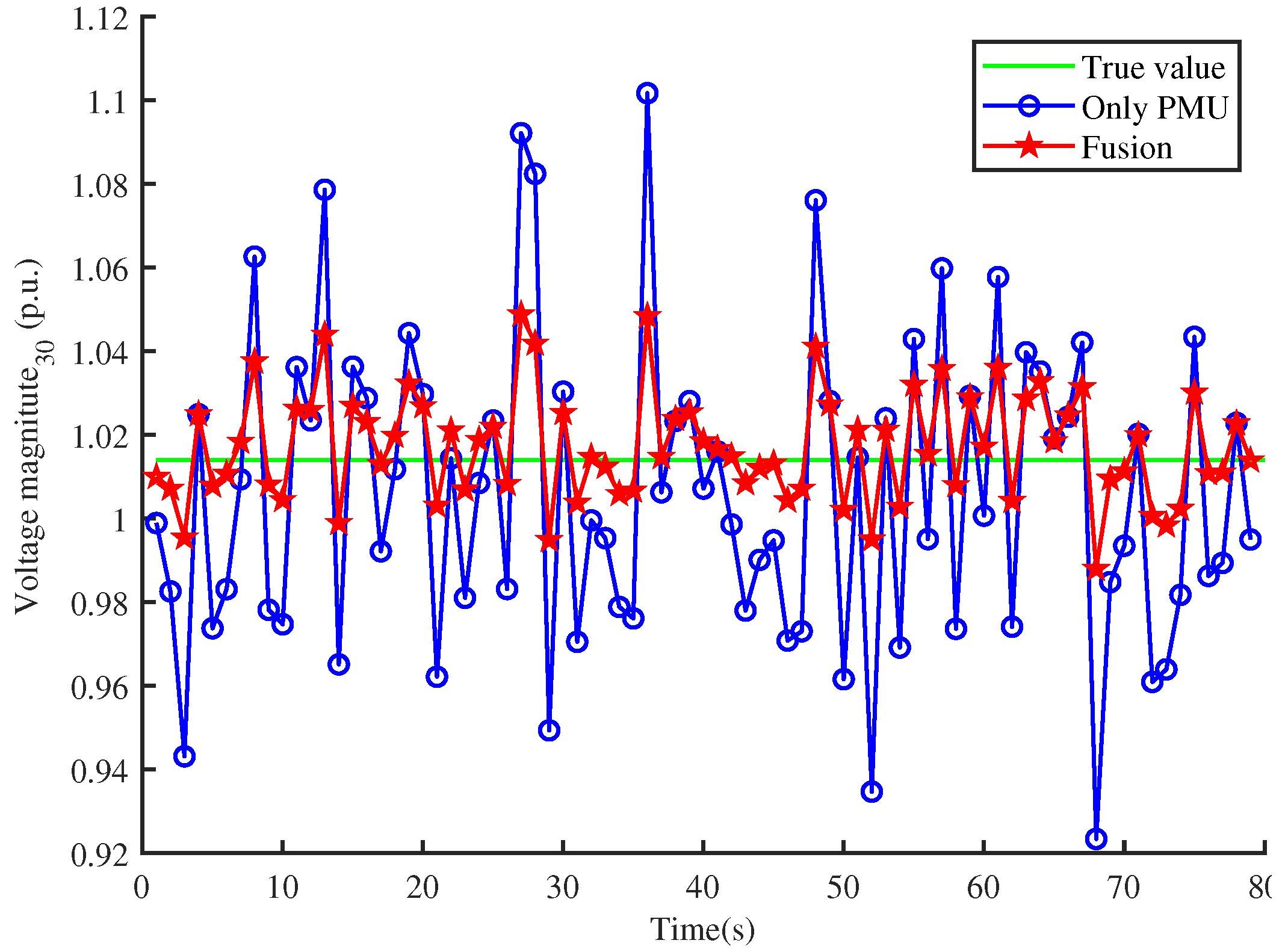
In order to avoid the influence of chance on the simulation experiment, the experiment is conducted in two power systems, respectively, to better determine the accuracy of the simulation experiment. Figure 5 and Figure 6 show the state estimation result graphs of the PMU-only estimator and the fusion estimator at a single node, which is node No. 8 in the IEEE-14 bus system and node No. 28 in the IEEE-30 bus system, respectively. These graphs show the estimator’s state estimation results at a single node at all moments during the iterative computation process.
Based on the power flow calculations, the true voltage magnitude at bus 8 in the IEEE-14 system should be 1.610 p.u. During the iterative process, this value is used as the baseline to compare the performance of the PMU-only estimator and the fusion estimator. From Figure 5 and Figure 6, it can be clearly seen that in the iterative process, the fusion estimator’s estimates at individual nodes are all closer to the true value than that of the PMU-only estimator, which also indicates that the fusion estimator has a better performance in the estimation process. The errors in the state estimates of the PMU and the SCADA are averaged, and the results are shown in Table 2, where it can be seen that the accuracy of the estimator that contains only the PMU is better than that of the estimator that contains only the SCADA estimator.
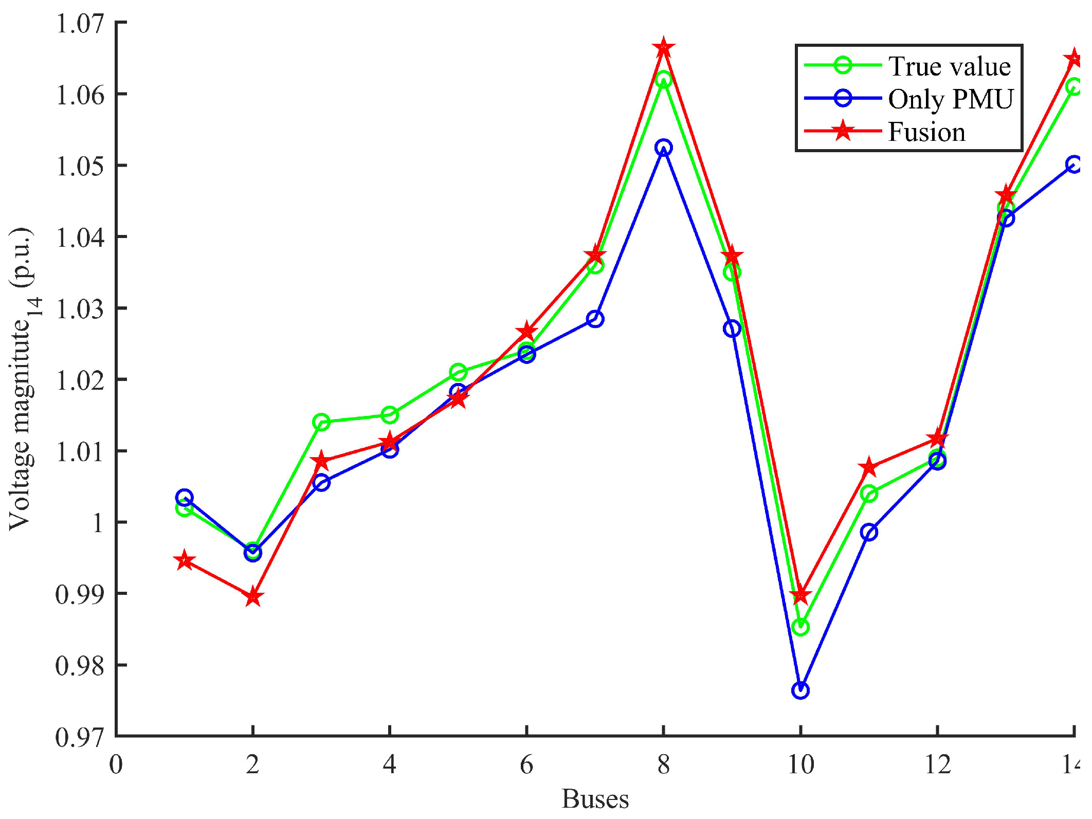
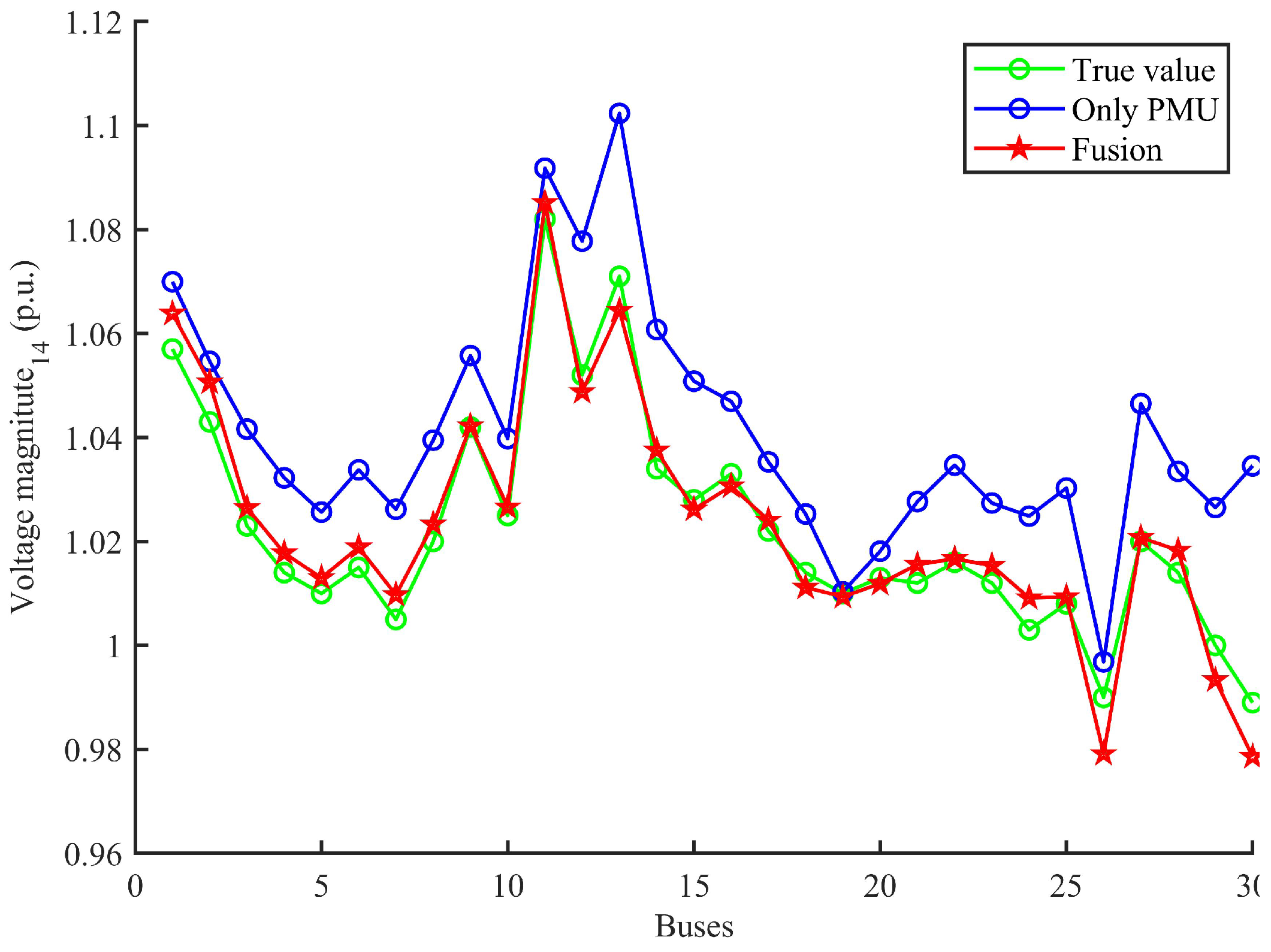
It is important to note that the selection of nodes was random. This was done to demonstrate that the performance of the fused estimator over various time periods in the filtering process is superior to that of individual estimators, and, therefore, does not carry any specific significance. In the IEEE-14 system, we could select any node from 1 to 14. However, in the IEEE-30 system, to better distinguish between different systems, we conducted random selections from nodes 15 to 30. Other nodes also exhibit similarly good performance, as illustrated in Figure 7 and Figure 8.
Figure 7 and Figure 8 show the state estimation effect of the estimator at each node of the IEEE-14 and IEEE-30 bus system at a certain moment of the iterative process. Added to the average PMU and SCADA estimation errors in Table 1, it is easy to see that the performance of the fusion estimator in performance in both power systems is better than the state estimation effect of a single estimator.

5.2. Analysis of Differentiation

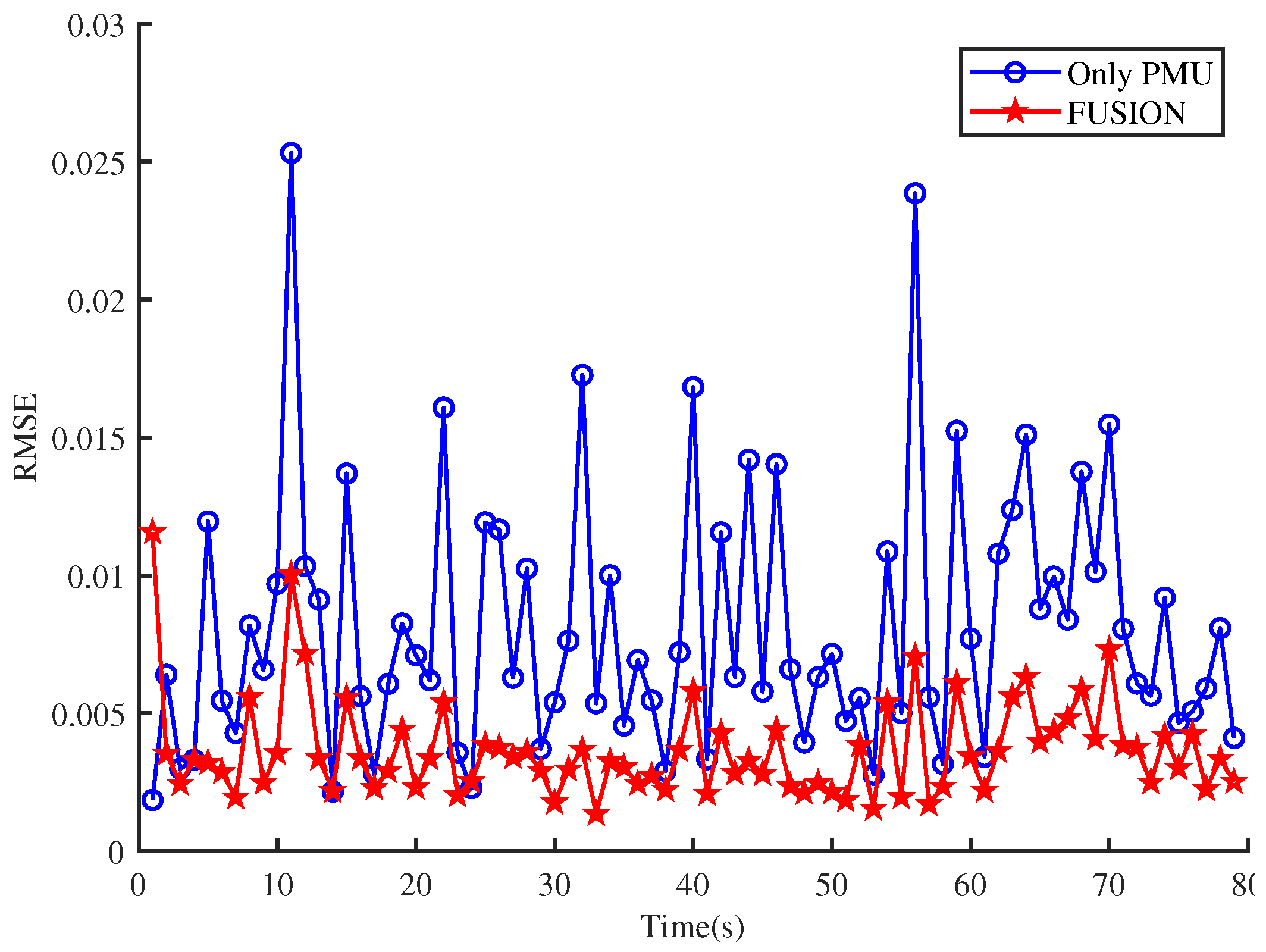
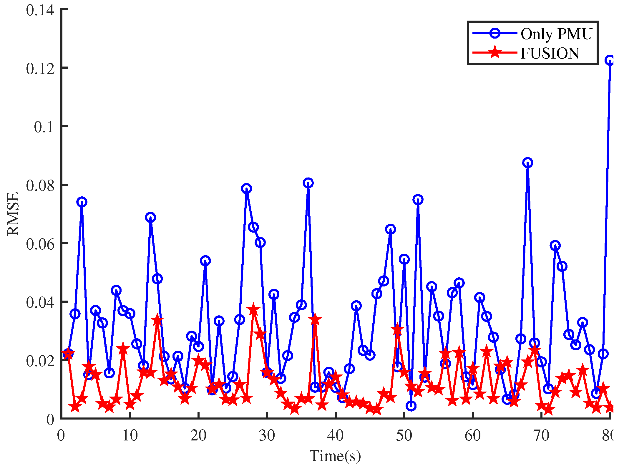
To ascertain the relative effectiveness of individual estimators compared to the fusion estimator, this study employs the root mean square error (RMSE) as a metric for evaluating estimation accuracy across the three estimators. RMSE quantifies the disparity between the predicted estimator and the actual value, thereby assessing the estimation error. Therefore, to better observe the superiority of the fusion estimator over that of PMUs alone, this subsection will focus on showcasing the performance differences between the PMU-only estimator and the fusion estimator.
As mentioned above, RMSE (Root Mean Square Error) is a commonly used performance evaluation metric used to measure the discrepancy between estimated values and actual values. In this section, RMSE represents the discrepancy between the estimated voltage state and the actual values. A smaller RMSE indicates better performance of the estimator, as it signifies a smaller discrepancy between estimated values and actual values. The RMSE is calculated as the square root of the average of the squared differences between the predicted and true values. This metric measures how much the predicted values deviate from the actual values and is particularly sensitive to outliers in the dataset.
RMSE = 1 m i = 1 m x ^ i x i 2
where m represents the total number of buses. The IEEE-14 and IEEE-30 bus systems are used for this simulation, so here m = 14 or m = 30 . i represents the bus number, i.e., i 1 m . x ^ i and x i , respectively, denote the estimated and actual values of voltage.
It is worth noting that the RMSE calculated here pertains to the amplitude of all nodes and illustrates the changes over an 80-second period in the simulation graph. Figure 9 and Figure 10, respectively, present the root mean square error values of estimators containing only PMUs and fusion estimators on the IEEE-14 and IEEE-30 bus systems. From the figures, it can be observed that regardless of whether on the 14-bus or the 30-bus system, the overall root mean square error of the fusion estimator is consistently smaller than that of the PMU estimator. This indicates that during the state estimation process, the state estimation results provided by the fusion estimator proposed in this paper exhibit smaller discrepancies from the true values.
From the above simulation experiments, it can be seen that although the performance of PMU estimation is superior to SCADA, the overall performance of the fusion estimator surpasses that of individual estimators. This is because the fusion estimator integrates the advantages of both PMUs and SCADA, incorporating the information from both estimators into one. As a result, during the state estimation process, the redundancy of system information is significantly increased. Hence, the obtained state estimation results are more accurate.
Additionally, when establishing new estimates, the KLA averaging method is employed. Consequently, the error covariance matrix of the new SCADA-based estimate x ^ s p is smaller compared to traditional SCADA estimates. Thus, integrating this newly estimated, lower-error value with PMUs will yield better results than traditional mixed estimation methods.

6. Conclusions

This paper introduces a novel fusion state estimator for power systems. Utilizing the KLA averaging distribution, this fusion estimator establishes a new SCADA-based estimation. This estimation process leverages PMU sampling times to estimate the state based on SCADA observations, effectively addressing the mismatch in sampling rates between SCADA and PMUs, a crucial factor in ensuring the accuracy of power system state estimation. In this study, the exponential smoothing method is used to neglect the step of estimating the initial state, and the initial state estimation can be determined quickly by weighted averaging the observed data, which reduces the computational time and complexity of the fusion process. The simulation results distinctly demonstrate that the fusion estimator proposed in this paper exhibits higher accuracy compared to estimators solely relying on PMU or SCADA data. This significant improvement highlights the efficacy of the proposed fusion method in enhancing the precision of power system state estimation.

Author Contributions

Conceptualization, J.Z.; methodology, Y.L. and W.G.; software, J.Z. and X.G.; validation, X.G.; formal analysis, X.G.; resources, W.G.; data curation, G.Z.; writing—original draft preparation, J.Z.; writing—review and editing, W.G. and Y.L.; visualization, G.Z. and W.S.; supervision, W.G.; project administration, Y.L.; funding acquisition, W.G. All authors have read and agreed to the published version of the manuscript.

Funding

This research was supported in part by the National Natural Science Foundation of China (NSFC) under Grant U21A20146, in part by the Collaborative Innovation Project of Anhui Universities under Grant GXXT-2020-070, in part by the Open Research Fund of Anhui Province Key Laboratory of Detection Technology and Energy Saving Devices under Grant JCKJ2022A10, and in part by the College Students’ Innovative Entrepreneurial Training Plan Program (202310363207).

Data Availability Statement

The Original contributions from the study are included in the article; for further enquiries, please contact the corresponding author.

Acknowledgments

All of us thank the anonymous reviewers for their valuable comments.

Conflicts of Interest

The authors declare no conflicts of interest.

References

  1. Jesus, P.M.D.O.; Rodriguez, N.A.; Celeita, D.F.; Ramos, G.A. PMU-Based System State Estimation for Multigrounded Distribution Systems. IEEE Trans. Power Syst. 2021, 36, 1071–1081. [Google Scholar] [CrossRef]
  2. Zhao, J.; Netto, M.; Huang, Z.; Yu, S.S.; Gómez-Expósito, A.; Wang, S.; Kamwa, I.; Akhlaghi, S.; Mili, L.; Terzija, V.; et al. Roles of Dynamic State Estimation in Power System Modeling, Monitoring and Operation. IEEE Trans. Power Syst. 2021, 36, 2462–2472. [Google Scholar] [CrossRef]
  3. Abooshahab, M.A.; Hovd, M.; Brekke, E.; Song, X. A Covariance Consistent Data Fusion method for Power Networks with Multirate Sensors. In Proceedings of the 2020 IEEE Conference on Control Technology and Applications (CCTA), Montreal, QC, Canada, 24–26 August 2020; pp. 807–814. [Google Scholar]
  4. Dobakhshari, A.S.; Azizi, S.; Paolone, M.; Terzija, V. Ultra Fast Linear State Estimation Utilizing SCADA Measurements. IEEE Trans. Power Syst. 2019, 34, 2622–2631. [Google Scholar] [CrossRef]
  5. Bose, A. Smart Transmission Grid Applications and Their Supporting Infrastructure. IEEE Trans. Smart Grid. 2010, 1, 11–19. [Google Scholar] [CrossRef]
  6. Dong, Q.; Sun, J.; Wu, Q.; Liu, Y. A Method for Filtering Low Frequency Disturbance in PMU Data Before Coordinated Usage in SCADA. IEEE Trans. Power Syst. 2017, 32, 2810–2816. [Google Scholar] [CrossRef]
  7. Cheng, G.; Lin, Y.; Zhao, J.; Yan, J. A Two-Stage State Estimator for Dynamic Monitoring of Power Systems. IEEE Trans. J. 2017, 11, 1767–1776. [Google Scholar]
  8. Zhou, N.; Meng, D.; Huang, Z.; Welch, G. Dynamic state estimation of a synchronous machine using PMU data: A comparative study. IEEE Trans. Smart Grid. 2015, 6, 450–460. [Google Scholar] [CrossRef]
  9. Sun, K.; Huang, M.; Wei, Z.; Zhao, J.; Sun, G. A Real-Time Recursion Correction Hybrid Linear State Estimator Using Stream Processing. IEEE Trans. Ind. Inf. 2023, 19, 2317–2329. [Google Scholar] [CrossRef]
  10. Sun, K.; Huang, M.; Wei, Z.; Sun, G. High-Refresh-Rate Robust State Estimation Based on Recursive Correction for Large-Scale Power Systems. IEEE Trans. Instrum. Meas. 2023, 72, 9002413. [Google Scholar] [CrossRef]
  11. Jorjani, M.; Seifi, H.; Varjani, A.Y. SCADA and PMU Measurements for Improving Power System State Estimation. IEEE Lat. Am. Trans. 2015, 13, 2245–2251. [Google Scholar]
  12. Kabiri, M.; Amjady, N. A New Hybrid State Estimation Considering Different Accuracy Levels of PMU and SCADA Measurements. IEEE Trans. Instrum. Meas. 2019, 68, 3078–3089. [Google Scholar] [CrossRef]
  13. Du, J.; Ma, S.; Wu, Y.-C.; Poor, H.V. Distributed Hybrid Power State Estimation Under PMU Sampling Phase Errors. IEEE Trans. Signal Process. 2014, 62, 4052–4063. [Google Scholar] [CrossRef]
  14. Rabha, P.; Shyam, C.C.; Sinha, A.K. Hybrid state estimation of power system using conventional and phasor measurements. In Proceedings of the 2015 International Conference on Energy, Power and Environment: Towards Sustainable Growth (ICEPE), Shillong, India, 12–13 June 2015; pp. 1–6. [Google Scholar]
  15. Albuquerque, A.; Bez, D.; Simões, A. Multistage strategies to incorporate phasor measurements into power system state estimation. In Proceedings of the 2013 IREP Symposium Bulk Power System Dynamics and Control—IX Optimization, Security and Control of the Emerging Power Grid, Rethymno, Greece, 25–30 August 2013; pp. 1–11. [Google Scholar]
  16. Netto, M.; Zhao, J.; Mili, L. A robust extended Kalman filter for power system dynamic state estimation using PMU measurements. In Proceedings of the 2016 IEEE Power and Energy Society General Meeting (PESGM), Boston, MA, USA, 17–21 July 2016; pp. 1–5. [Google Scholar]
  17. Aminifar, F.; Shahidehpour, M.; Fotuhi-Firuzabad, M.; Kamalinia, S. Power System Dynamic State Estimation With Synchronized Phasor Measurements. IEEE Trans. Instrum. Meas. 2014, 63, 352–363. [Google Scholar] [CrossRef]
  18. Bi, T.S.; Qin, X.H.; Yang, Q.X. A novel hybrid state estimator for including synchronized phasor measurements. Electr. Power Syst. Res. 2018, 78, 1343–1352. [Google Scholar] [CrossRef]
  19. Ghosal, M.; Rao, V. Fusion of Multirate Measurements for Nonlinear Dynamic State Estimation of the Power Systemss. IEEE Trans. Smart Grid. 2019, 10, 216–226. [Google Scholar] [CrossRef]
  20. Li, Z.; Li, S.; Liu, B.; Yu, S.S.; Shi, P. A Stochastic Event-Triggered Robust Cubature Kalman Filtering Approach to Power System Dynamic State Estimation with Non–Gaussian Measurement Noises. IEEE Trans. Contr. Syst. Technol. 2023, 31, 889–896. [Google Scholar] [CrossRef]
  21. Zhao, J.; Gómez-Expósito, A.; Netto, M.; Mili, L.; Abur, A.; Terzija, V.; Kamwa, I.; Pal, B.; Singh, A.K.; Qi, J.; et al. Sakis Power System Dynamic State Estimation: Motivations, Definitions, Methodologies, and Future Work. IEEE Trans. Power Syst. 2019, 34, 3188–3198. [Google Scholar] [CrossRef]
  22. Kong, X.; Zhang, X.; Zhang, X.; Wang, C.; Chiang, H.-D.; Li, P. Adaptive Dynamic State Estimation of Distribution Network Based on Interacting Multiple Model. IEEE Trans. Sustain. Energy 2022, 13, 643–652. [Google Scholar] [CrossRef]
  23. Abur, A.; Expoisito, A.G. Power System State Estimation: Theory and Implementation, 1st ed.; Marcel Dekker: New York, NY, USA, 2004. [Google Scholar]
  24. Liu, H.; Liang, F.; Hu, T.; Hong, J.; Ma, H. Multi-Scale Fusion Model Based on Gated Recurrent Unit for Enhancing Prediction Accuracy of State-of-Charge in Battery Energy Storage Systems. J. Mod. Power Syst. Clean Energy 2024, 12, 405–414. [Google Scholar] [CrossRef]
  25. Cristi, R.; Tummala, M. Multirate, multiresolution, recursive Kalman filter. Signal Process. 2000, 80, 1945–1958. [Google Scholar] [CrossRef]
  26. Chen, J.; Yue, D.; Hu, S.; Ge, H.; Zhang, H. Power System Fusion State Estimation Based on a Switched System Model: Comparison Between EKF and UKF. In Proceedings of the 2019 Chinese Control Conference (CCC), Guangzhou, China, 27–30 July 2019; pp. 7280–7284. [Google Scholar]
  27. Kiio, M.N.; Wekesa, C.W.; Kamau, S.I. Evaluating Performance of a Linear Hybrid State Estimator Utilizing Measurements from RTUs and Optimally Placed PMUs. IEEE Access 2022, 10, 63113–63131. [Google Scholar] [CrossRef]
  28. He, Y.; Mendis, G.J.; Wei, J. Observability Analysis and Measurement Placement for Systems with PMUs. In Proceedings of the 2014 International Conference on Computing, Networking and Communications (ICNC), New York, NY, USA, 10–13 October 2004; pp. 943–946. [Google Scholar]
  29. Göl, M.; Abur, A. A Hybrid State Estimator For Systems With Limited Number of PMUs. IEEE Trans. Power Syst. 2015, 30, 1511–1517. [Google Scholar] [CrossRef]
  30. Wakti, M.H.; Putranto, L.M.; Hadi, S.P.; Yasirroni, M.; Marsiano, A.F.D. PMU Location Determination in a Hybrid PMU-SCADA System. In Proceedings of the 2020 12th International Conference on Information Technology and Electrical Engineering (ICITEE), Yogyakarta, Indonesia, 6–8 July 2020; pp. 245–250. [Google Scholar]
  31. Simões Costa, A.; Albuquerque, A.; Bez, D. An estimation fusion method for including phasor measurements into power system real-time modeling. IEEE Trans. Power Syst. 2013, 28, 1910–1920. [Google Scholar] [CrossRef]
  32. Moslemi, R.; Mesbahi, A.; Velni, J.M. The Effect of the Common Process Noise on the Two-Sensor Fused-Track Covariance. IEEE Trans. Aerosp. Electron. Syst. 1986, 22, 803–805. [Google Scholar]
  33. Chen, Y.; Huang, S.; Liu, F.; Wang, Z.; Sun, X. Enhancement of hybrid state estimation using pseudo flow measurements. In Proceedings of the 2011 IEEE Power and Energy Society General Meeting, Detroit, MI, USA, 24–28 July 2011; pp. 1–7. [Google Scholar]
  34. Zimmerman, R.D.; Murillo-Sánchez, C.E.; Thomas, R.J. MATPOWER: Steady-State Operations, Planning, and Analysis Tools for Power Systems Research and Education. IEEE Trans. Power Syst. 2011, 26, 12–19. [Google Scholar] [CrossRef]
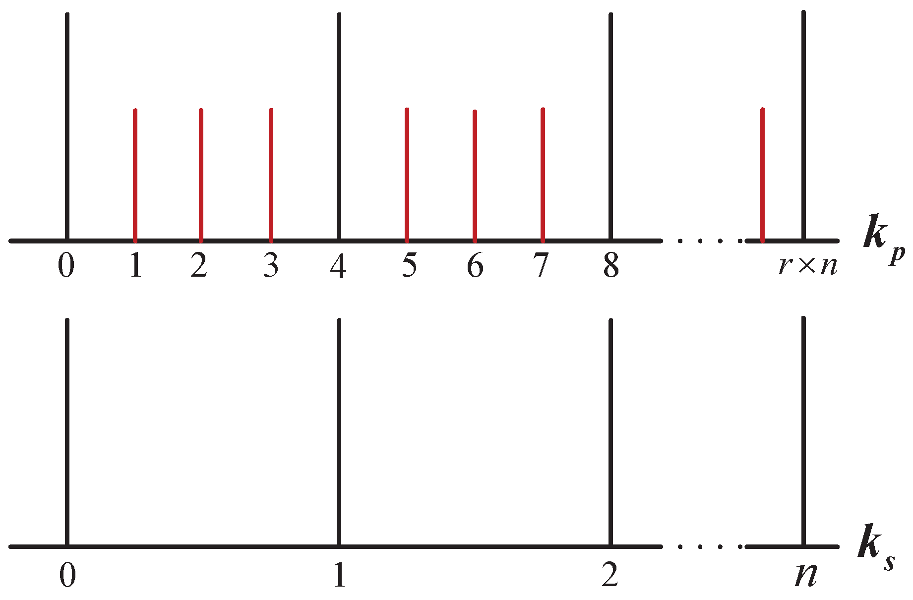
Figure 1. PMU and SCADA Measurement Instantaneous Comparison.
Energies 17 02609 g001
Figure 2. The Execution Process of the Fusion Algorithm.
Energies 17 02609 g002
Figure 3. PMU Placement on IEEE-14 Bus System.
Energies 17 02609 g003
Figure 4. PMU Placement on IEEE-30 Bus System.
Energies 17 02609 g004
Figure 5. The voltage magnitude at Node 8 before and after fusion in the IEEE-14 bus system.
Energies 17 02609 g005
Figure 6. The voltage magnitude at Node 28 before and after fusion in the IEEE-30 bus system.
Energies 17 02609 g006
Figure 7. The voltage magnitude state estimation results for the IEEE-14 bus system.
Energies 17 02609 g007
Figure 8. The voltage magnitude state estimation results for the IEEE-30 bus system.
Energies 17 02609 g008
Figure 9. Root Mean Square Error (RMSE) of Individual Estimator (PMU-Only) and Fused Estimator State Estimation in the IEEE-14 Bus System.
Energies 17 02609 g009
Figure 10. Root Mean Square Error (RMSE) of Individual Estimator (PMU-Only) and Fused Estimator State Estimation in the IEEE-30 Bus System.
Energies 17 02609 g010
Table 1. Phasor Measurement Data.
TypeMagnAngleFrom BusTo Bus
Voltage Phasor 1.0450 0.0871 20
1.0700 0.2521 60
1.0457 0.2310 70
1.0305 0.2587 90
Current Phasor 1.4910 3.0307 21
0.7046 0.1678 23
0.5361 0.1395 24
0.4019 0.2001 25
0.1136 1.0730 611
0.0810 0.6273 612
0.1951 0.7506 613
0.1947 1.3398 78
0.2950 0.7314 79
0.0435 0.0556 910
1.0305 0.2959 914
Table 2. Comparison of Average Estimation Errors between SCADA and the PMUs.
BusesSCADA (p.u.)PMU (p.u.)
IEEE-14 5.23 × 10 2 7.35 × 10 3
IEEE-30 8.12 × 10 2 2.64 × 10 3
Disclaimer/Publisher’s Note: The statements, opinions and data contained in all publications are solely those of the individual author(s) and contributor(s) and not of MDPI and/or the editor(s). MDPI and/or the editor(s) disclaim responsibility for any injury to people or property resulting from any ideas, methods, instructions or products referred to in the content.