An Improved WOA (Whale Optimization Algorithm)-Based CNN-BIGRU-CBAM Model and Its Application to Short-Term Power Load Forecasting

Abstract

The accuracy requirements for short-term power load forecasting have been increasing due to the rapid development of the electric power industry. Nevertheless, the short-term load exhibits both elasticity and instability characteristics, posing challenges for accurate load forecasting. Meanwhile, the traditional prediction model suffers from the issues of inadequate precision and inefficient training. In this work, a proposed model called IWOA-CNN-BIGRU-CBAM is introduced. To solve the problem of the Squeeze-and-Excitation (SE) attention mechanism’s inability to collect information in the spatial dimension effectively, the Convolutional Block Attention Module (CBAM) is firstly introduced as a replacement. This change aims to enhance the ability to capture location attributes. Subsequently, we propose an improved Whale Optimization Algorithm (IWOA) that addresses its limitations, such as heavy reliance on the initial solution and susceptibility to local optimum solutions. The proposed IWOA is also applied for the hyperparameter optimization of the Convolutional Neural Network–Bidirectional Gated Recurrent Unit–Convolutional Block Attention Module (CNN-BiGRU-CBAM) to improve the precision of predictions. Ultimately, applying the proposed model to forecast short-term power demand yields results that show that the CBAM effectively addresses the problem of the SE attention mechanism’s inability to capture spatial characteristics fully. The proposed IWOA exhibits a homogeneous dispersion of the initial population and an effective capability to identify the optimal solution. Compared to other models, the proposed model improves R² by 0.00224, reduces the RMSE by 18.5781, and reduces MAE by 25.8940, and the model’s applicability and superiority are validated.

1. Introduction

Accurate load forecasting has become crucial in dispatching power to satisfy customer demands, load switching, and infrastructure expansion as modern energy systems become increasingly complex and flexible [1]. Short-term power load forecasting (STLF) is essential for the smooth functioning of the power system, and precise load prediction is crucial for guaranteeing the secure and steady operation of the power system [2]. The significance of predicting short-term load has increased with the advancement of the power industry. Nevertheless, the immediate demand exhibits characteristics of elasticity and unpredictability, resulting in increased challenges in accurate load forecasting.

Researchers have provided a variety of models in the past decades to make more accurate short-term load forecasts. The methods mainly consist of traditional methods for forecasting and artificial intelligence methods [3]. Conventional approaches to STLF primarily include the ARIMA model [4], the grey model (GM) [5], and the Kalman filtering method [6]. The ARIMA model is a statistical model based on time-series data, commonly used for analysing and forecasting trends and periodicity in time-series data. The Grey Model (GM) is a modelling method based on a small amount of data, particularly suitable for predicting when there is insufficient data support. Kalman filtering is a recursive filtering technique used to estimate system states, particularly suitable for systems with dynamic changes. These three methods have their advantages and limitations in dealing with different types of load data and forecasting periods. The ARIMA model is suitable for stable load data and short-term forecasts, but may perform poorly for nonlinear and dynamically changing load data; the GM method is suitable for situations with fewer data or slow load changes, but may be insufficient for handling rapid changes and complex data; the Kalman filtering method is suitable for situations that require consideration of system dynamic changes and time variations, but requires a good understanding and modelling of the system’s state space model. Additionally, due to the non-linear characteristics of load data, the above traditional forecasting methods encounter difficulties in accurately predicting load trends. In power systems, load data characteristics are complex and variable, with nonlinear features being particularly prominent. The nonlinearity of load data is primarily reflected in the following aspects: (1) Complexity of load demand: Power load demand is influenced by numerous factors, including temperature, humidity, seasonal changes, and economic activities. These factors have complex nonlinear relationships, causing power load to exhibit significant nonlinear characteristics. (2) Diversity of user behaviour: Different users exhibit varying electricity usage behaviours, with industrial, commercial, and residential users showing distinct usage patterns. This behavioural diversity makes the nonlinear characteristics of load data more complex. (3) Dynamic characteristics of power systems: The power system itself is a complex dynamic system. The start-up and shutdown of generation equipment, faults, and maintenance all cause fluctuations in load. Additionally, mechanisms for supply and demand balance in the power market, and real-time price fluctuations also impart nonlinear effects on load data.

Therefore, scholars have proposed artificial intelligence methods. Artificial intelligence (AI) techniques have recently seen increased use in STLF, which include Support Vector Machine (SVM) [7], Long Short-Term Memory (LSTM) network [8], Bi-directional Long Short-Term Memory (BiLSTM) [9], Gated Recurrent Unit (GRU) [10] network, and the improved models of various scholars, etc., which can capture the non-linear characteristics of power loads better and significantly enhance the precision of load forecasting. BiGRU [11] can consider past and future known data and learn more feature information effectively. Most of these single neural network models make predictions for time series. However, a single neural network model produces inferior forecasts in intricate tasks as it neglects to account for the spatial correlations among data points.

Further, extracting spatiotemporal features in load data can provide more comprehensive and accurate data, thus helping to capture the characteristics of load changes at a finer level and improve prediction accuracy. CNN-BiGRU [12] improves prediction accuracy by introducing a CNN layer to extract intricate high-dimensional spatio-temporal features. The CNN-BiGRU-Attention model enhances its prediction accuracy by incorporating the SE-Attention mechanism into the CNN-BiGRU model. However, factors such as the inability of the SE-Attention mechanism to capture valid information in the spatial dimension and the high human interference in the model parameters lead to poor prediction accuracy of the CNN-BiGRU-Attention.

The issue of selecting hyperparameters for the model can be considered an optimization problem, which is generally optimized using exact algorithms such as the Bayesian optimization algorithm [13], Adam’s algorithm [14], or heuristic algorithms. The exact approach can yield a precise solution. However, the efficiency of the solution is not good. Heuristic algorithms like Grey Wolf Optimizer (GWO) [15] and Particle Swarm Optimization (PSO) have the advantages of being highly effective in finding the optimal solution and having greater optimization efficiency, making them more competitive. Nevertheless, heuristic algorithms exhibit certain limitations. For instance, the GWO algorithm has inadequate population diversity and limited global search capability.

Similarly, the PSO algorithm exhibits a deceleration in convergence as the search progresses toward its later phases and is prone to becoming trapped in optimal local settings. Mirjalili and Lewis introduced the WOA [16] heuristic optimization algorithm in 2016, with good global search performance, few control parameters, ease of implementation, etc. Consequently, it has gained popularity in various problem-solving domains, such as combinatorial optimization, image segmentation, data prediction, path planning, etc. However, WOA also suffers from the problems of being sensitive to parameters, possibly falling into a local optimal solution, and having a strong dependence on the initial solution.

In summary, an IWOA-CNN-BIGRU-CBAM model is introduced in this paper. To mitigate the limitation of the SE attention mechanism to scenes with a greater number of channels and its inability to capture spatio-temporal features effectively, the CBAM is implemented as an alternative to enhance the capability of capturing such features. Meanwhile, considering the drawbacks of WOA falling into local optimal solutions and the strong dependence on the initial solution, an improved WOA is proposed. The improved WOA is applied to hyperparameter optimization of CNN-BiGRU-CBAM to enhance the accuracy of predictions. The proposed approach exhibits exceptional precision and effectiveness, making it well-suited for addressing issues such as the inadequate accuracy of STLF. This study contributes the following.

• Aiming at the problem that the CNN-BiGRU-Attention model cannot capture adequate information in the spatial dimension, the CBAM is implemented to boost the model’s capacity to capture positional information.
• Considering that WOA has the shortcomings of being sensitive to parameters, dependent on the initial solution, and easily falling into local optimal solutions, an improved WOA is proposed, which, by introducing good point sets, improved convergence factors, and mutation mechanisms, boosts the optimization potential of WOA.
• Through experiments, this study presents a model that achieves high levels of prediction accuracy and high training efficiency. Compared with models such as BiLSTM, RMSE and MAE decreased by 291.9470 and 219.9830, respectively, and R² improved by 0.06941.

2. Related Work

The traditional methods for power load forecasting mainly include the ARIMA model, the grey model (GM), and the improved models of various scholars. For example, scholars such as Fei Wu [17] proposed a fractional autoregressive integral moving average (FARIMA) model optimized with the cuckoo search (CS) algorithm, and scholars such as Saadat Bahrami [18] formulated a model integrating the WT (wavelet transform) and GM optimized with the PSO algorithm. Similarly, there are linear regression and non-linear regression models [19]. The ARIMA model is suitable for linear data and is easy to implement, but it performs poorly with nonlinear data and long-term forecasting. The Grey Model (GM) adapts well to small samples and uncertain systems, but it has limited prediction accuracy and capability to handle abrupt data changes. The FARIMA model optimized with the Cuckoo Search (CS) algorithm and the integrated model of Wavelet Transform (WT) and Grey Model (GM) optimized with the Particle Swarm Optimization (PSO) algorithm excel in handling complex data and improving prediction accuracy. However, they have high computational complexity and difficulty in parameter tuning. Linear and nonlinear regression models are simple and intuitive, widely applied, but the former lacks the ability to handle nonlinear relationships, while the latter is more complex in model selection and parameter tuning. The continuous development of these methods has improved the accuracy of power load forecasting, but their respective limitations still need to be comprehensively considered in practical applications.

AI techniques for STLF have grown in popularity in the last several years. For instance, machine learning-based approaches have been employed, including Support Vector Machines (SVM) [20,21], Random Forest (RF) and eXtreme Gradient Boosting (XGBoost) [22]; artificial neural networks (ANN), BP neural networks [23,24], the deep neural network (DNN) algorithm [25] and deep learning-based methods are also used, including the Gated Recurrent Unit (GRU), Long Short-Term Memory (LSTM), Convolutional Neural Network (CNN), and improved models by various scholars, etc. These methods show broad application prospects in short-term load forecasting. Machine learning methods such as Support Vector Machines (SVM), Random Forest (RF), Extreme Gradient Boosting (XGBoost), etc., can handle complex nonlinear relationships, while deep learning methods such as Gated Recurrent Unit (GRU), Long Short-Term Memory (LSTM), Convolutional Neural Network (CNN), etc., can effectively extract spatio-temporal features. Model fusion and improved structures also bring new ideas for improving prediction accuracy. However, these methods still face challenges in terms of computational complexity, parameter tuning, and handling high-dimensional nonlinear data, which require further research and improvement.

Accordingly, scholars such as Mu Yangyang [26] improved prediction accuracy by combining the sequence-to-sequence structure with LSTM. Fang Liu [27] and other scholars proposed an ultra-short-term power load-forecasting model by integrating an attention mechanism, BiLSTM, and CNN, which extracts load data-related spatio-temporal features using CNN and BiLSTM. Wu Kuihua [28] and other scholars suggested a model for STLF that integrates LSTM and BiLSTM with an attention-based CNN. The combination prediction model based on the LSTM module faces challenges when dealing with long sequential data, such as high computational complexity, difficulty in capturing long-term dependencies, and high memory consumption. The GRU model was introduced with a simpler structure and fewer parameters. The GRU model improves training speed and computational efficiency while maintaining performance, making it widely used in sequence modelling tasks. Scholars such as Jia Taorong [29] have suggested a method for predicting short-term power load using a combination of CEEMDAN, the Multiverse optimization (MVO) algorithm, and the GRU based on the Rectified Adam (RAdam) optimizer. Using the GRU as a foundation, the BiGRU model was further proposed to extract contextual information from sequence data more effectively. Liang Rong [30] and other scholars proposed an Adamax-BiGRU model using the Adamax optimization algorithm. Further, Zhang Chu [12] and other scholars proposed an integrated multivariate PV power prediction model incorporating VMD, CNN, and BiGRU with full consideration of load data’s geographical and chronological aspects. Then, the attention mechanism can notably enhance the predictive efficacy of the model by allocating distinct weights to the crucial information. Meng Yuyu [31] and other scholars proposed an ACNN-BiGRU wind power ultrashort-term prediction model, which applies a CNN to extract important spatio-temporal properties from the input data. Xu Yucheng [32] and other scholars proposed a hybrid model called BiGRU-SENet, which incorporates the attention mechanism. This model is particularly effective in handling the nonlinearities found in high-dimensional time-series data. The SE attention mechanism, however, cannot capture adequate information in the spatial dimension, which applies to the problem of scenarios with more channels, and its computational efficiency is not high.

The prediction model training process involves many parameters, which can be an optimization issue. Currently, it is generally solved by exact optimization algorithms or heuristic algorithms. Biao Yang [33] and other scholars built a Bayes-BiLSTM model by optimizing the BiLSTM parameters utilizing a Bayesian optimization technique. Dashe Li [14] and other scholars established the Enhanced Clustering Algorithm and Adam-based Radial Basis Function Neural Network (ECA-Adam-RBFNN). Although it produces accurate solutions, the precise approach is inefficient because it relies too much on gradient information. The heuristic algorithm is more competitive with the advantages of optimality-seeking solid ability, faster training efficiency, higher optimization efficiency, and shorter solution time. Scholars such as Mengdan Feng [34] developed the GWO-XGBOOST-CEEMDAN model for carbon price forecasting by optimizing the parameters of the XGBOOST model utilizing the GWO algorithm. However, the GWO algorithm has poor population diversity and weak global search ability. Jun Guo [35] and other scholars established the PSO-GRU model to forecast air-mining coal temperatures; Manzhe Xiao [36] and other scholars proposed an enhanced BP neural network based on the PSO algorithm to predict carbon price. The PSO algorithm slows the convergence speed in the late stage of the search, and it is rather simple to become stuck in the local optimum. The WOA has the advantages of good global search performance and easy implementation, etc. Luo Jun [37] and other scholars proposed an ARIMA-WOA-LSTM model, where WOA is applied for hyper-parameter optimization of the LSTM. Sun Youzhuang [38] and others developed a WOA-Elman model. These research methods demonstrate the potential of combining optimization algorithms with neural network models in various fields. By utilizing optimization algorithms to adjust model parameters, researchers have successfully improved the performance of prediction models. The advantage of this approach lies in its ability to better adapt to complex data structures and achieve more accurate results in prediction tasks. However, some optimization algorithms such as GWO and PSO have limitations in terms of population diversity and global search, which may result in slow convergence or convergence to local optima. Therefore, future research needs to further improve these algorithms to enhance their efficiency and robustness in optimizing prediction models.

3. Model and Methodology

3.1. CNN-BiGRU-CBAM

Figure 1 shows the architecture of the CNN-BiGRU-CBAM model. Figure 1 illustrates that after the historical load data are entered from the input layer, they enter the CNN network layer, where features are extracted. Data correlation is captured utilizing the convolutional layer. Network learning efficiency is enhanced by using the pooling layer, which reduces data dimensionality via pooling operations. The CBAM module facilitates the model’s learning and extraction of local features and the extended memorable features in the data. Then, the data enter the BiGRU network, and the processed data are fully learned, further improving spatio-temporal feature extraction accuracy. Ultimately, the fully interconnected layer generates final forecasting outcomes.

3.1.1. CNN

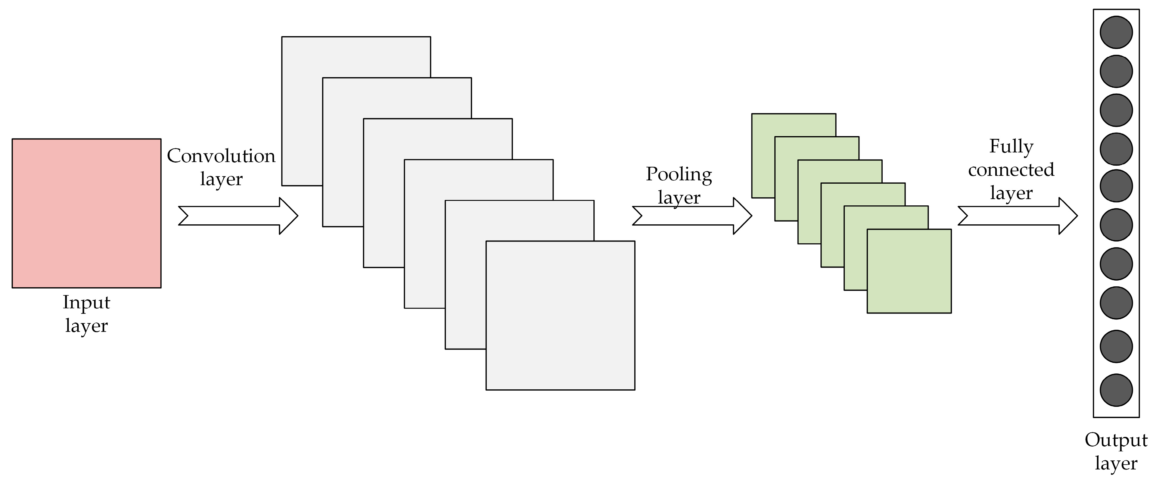
Convolutional neural networks (CNN) [39] are a subtype of feed-forward neural networks characterized by their deep architecture and incorporation of convolution processing. They frequently address overfitting, inefficiency, and spatial data loss. Figure 2 presents the CNN structure.

The CNN model structure can automatically extract features at different levels and scales by combining convolutional and pooling layers, enabling efficient feature-learning and classification tasks.

3.1.2. BiGRU

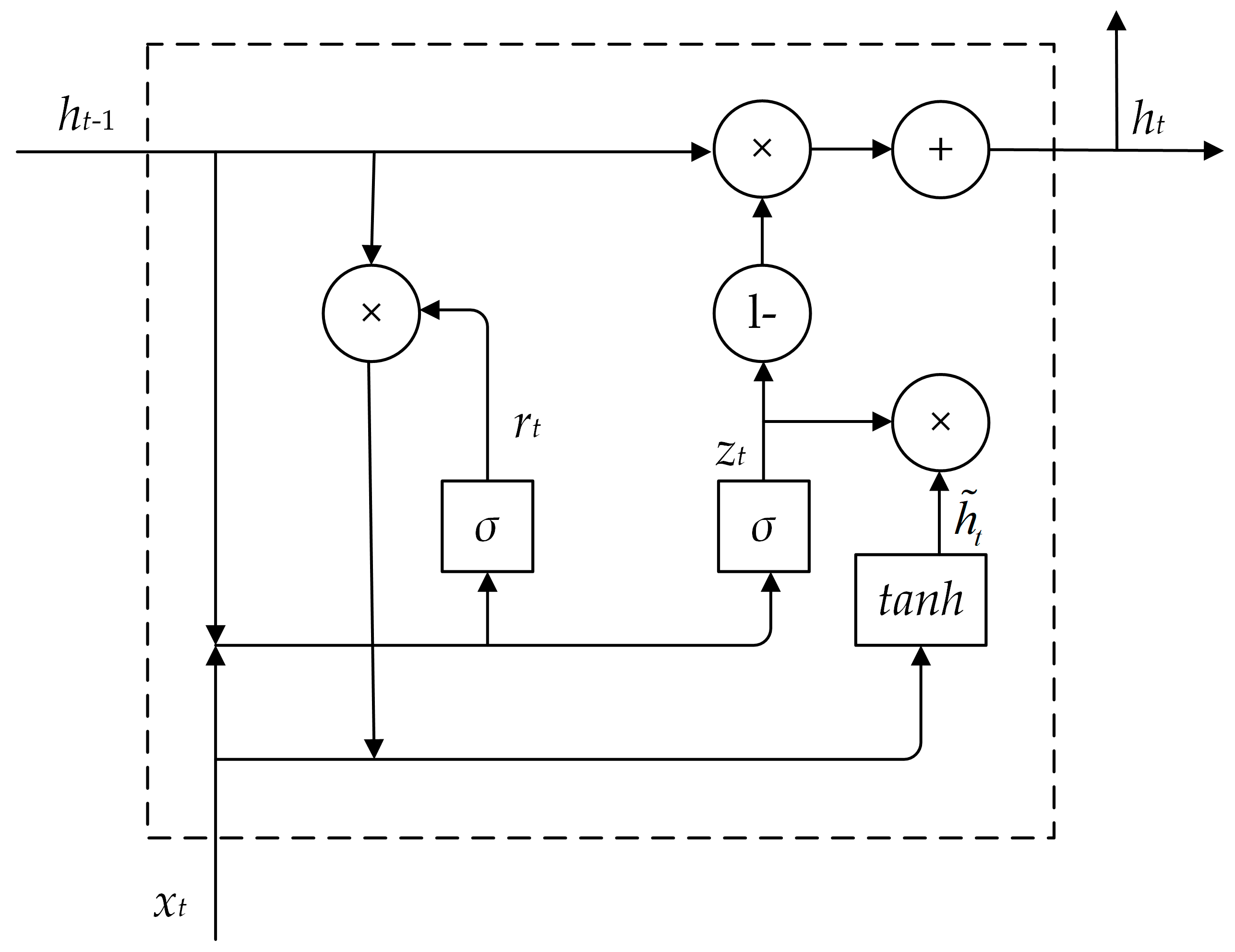
BIGRU [11] is a model that utilizes the deep learning algorithm to process sequence data. It is based on improving GRU [40] to better capture contextual information in sequence data by introducing a bidirectional loop structure. Each BiGRU unit contains two gated loop units, one dedicated to forward-direction sequence data processing and the other to reverse-direction sequence data processing. These two directional units can capture different information in the sequence and combine them to provide a more comprehensive contextual understanding. Figure 3 illustrates the structure of the GRU, and Figure 4 depicts the BiGRU structure.

A GRU (Gated Recurrent Unit) [39] consists of update gate $z_t$ and reset gate $r_t$, which combines the input gate and forgetting gate in LSTM into a single update gate, which reduces the training parameters of the model and the model convergence time, reduces the training complexity, and has fewer parameters and faster convergence time during training.

$$r_t=\sigma \left(W_r{x}_t+U_r{h}_{t-1}\right)$$

(1)

$$z_t=\sigma \left(W_z{x}_t+U_z{h}_{t-1}\right)$$

(2)

$$\widetilde{h_t}=\tanh \left(W{x}_t+U\left(r_t\odot h_{t-1}\right)\right)$$

(3)

$$h_t=\left(1-z_t\right)h_{t-1}+z_t\widetilde{h_t}$$

(4)

where $W_t$, $W_z$, $W$, $U_r$, $U_z$, $U$ are the weight matrix of GRU. $\sigma$ denotes the logical sigmoid function; $tanh$ denotes the tanh function; $\odot$ denotes the element multiplication operation; $z_t$ denotes the update gate, which can decide the degree of updating of the activation value of the GRU unit, which is jointly decided by the input state and the state of the previous hidden layer; $r_t$ denotes the reset gate, whose updating process is similar to the process of $z_t$; $\widetilde{h_t}$ denotes the candidate hidden layer; and $h_t$ denotes the hidden layer.

3.1.3. CBAM (Convolutional Block Attention Module)

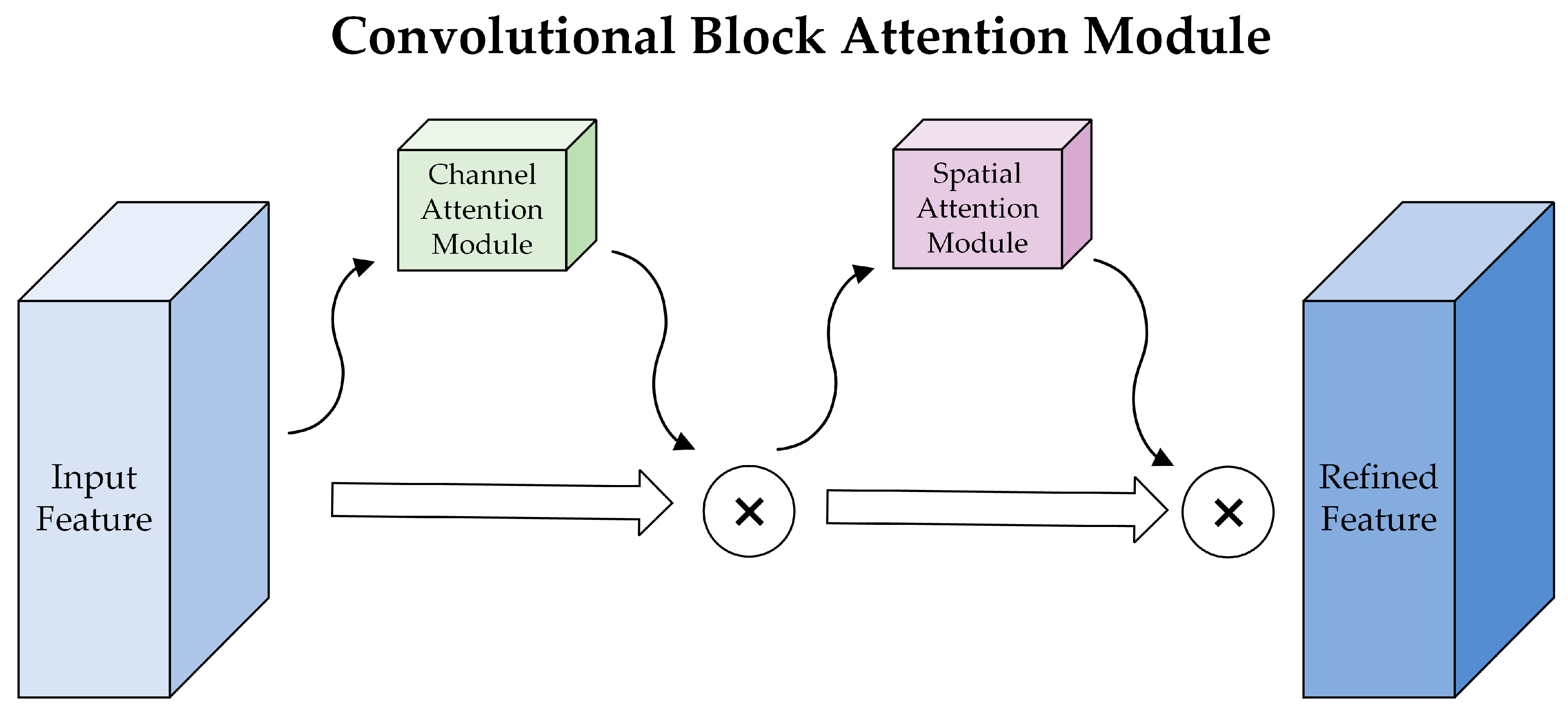
CBAM [41] is an attention mechanism used to enhance the efficiency of convolutional neural networks. The model’s representation capacity is enhanced by incorporating an attention mechanism into the convolutional block, allowing the model to prioritize the significant aspects of the input effectively. The CBAM architecture is illustrated in Figure 5.

Channel attention and spatial attention modules are the two sequential steps of the CBAM. The input feature map $F$ undergoes global maximum and global average pooling in the channel attention module to obtain $F_{avg}^c$ and $F_{\max }^c$, after the Share MLP module, channel attention, is generated. Next, element-wise addition is used to merge the output feature vectors, which are subjected to compression using a sigmoid function followed by multiplication with the original input feature map to obtain the weighted feature map. Notably, the structure can be observed in Figure 6. The formula for channel attention is displayed below.

$$\begin{array}{c}{M}_c\left(F\right)=\sigma \left(MLP\left(AvgPool\left(F\right)\right)+MLP\left(MaxPool\left(F\right)\right)\right)\\ =\sigma \left(W_1\left(W_0\left(F_{avg}^c\right)\right)+W_1\left(W_0\left(F_{\max }^c\right)\right)\right)\end{array}$$

(5)

By applying global maximum and global average pooling to the channel attention output, $F_{avg}^s$ and $F_{\max }^s$ can be obtained for the spatial attention module, after which the resulting feature maps are stacked and then made into one-channel feature maps by a convolutional layer, followed by compression by a sigmoid function and multiplication with the original input feature maps to obtain the weighted feature maps. Its resulting structure is illustrated in Figure 7. Below is the formula for spatial attention:

$$\begin{array}{c}{M}_s\left(F\right)=\sigma \left(f^{7\times 7}\left(\left[AvgPool\left(F\right);MaxPool\left(F\right)\right]\right)\right)\\ =\sigma \left(f^{7\times 7}\left(\left[F_{avg}^s;F_{\max }^s\right]\right)\right)\end{array}$$

(6)

The CBAM enables the model to dynamically acquire knowledge about the significance of each channel and location, hence enhancing the model’s capacity for expression. The CBAM exhibits clear advantages over the SE attention mechanism regarding channel characteristics, spatial characteristics, computational efficiency, and scalability.

Meanwhile, CBAM can handle the high-dimensional spatio-temporal features extracted by CNN, and the combination of the two can handle the spatio-temporal features well in load data. BiGRU does not take spatial correlations among data points into account. In this paper, the combination of CNN and CBAM is used to enhance the accuracy of predictions.

3.2. Improved Whale Optimization Algorithm (IWOA)

An IWOA is introduced to address its limitations, including sensitivity to parameters, susceptibility to local optimal solutions, and heavy reliance on the initial solution. The proposed algorithm incorporates strategies such as a friend variation mechanism, an improved convergence factor, and a suitable point set.

3.2.1. WOA

Mirjalili and Lewis developed the WOA, a heuristic optimization technique, in 2016 [16]. The hunting behaviour of humpback whales served as an inspiration for the algorithm, which was mathematically modelled by simulating the whales’ round-up behaviour and the attack mechanism of bubble-net foraging to achieve optimization. The WOA possesses the advantages of a smaller amount of control parameters, uncomplicated implementation, and an effective global search capability. This program follows a three-step process that mimics the distinctive search technique and feeding behaviour of humpback whales: prey seining, bubble net foraging, and prey searching. The WOA considers each location of humpback whales as a potential solution, and the optimal solution is obtained by consistently revising the whales’ locations within the solution space.

1.

Rounding up prey

WOA postulates that the present most favourable candidate solution is either the desired prey or a solution very close to optimal. After identifying the optimal search agent, subsequent search agents will strive to synchronize their positions with those of the highest-performing agent. The following formulae express this behaviour.

$$\overrightarrow{D}=\left|\overrightarrow{C}\cdot \overrightarrow{X^{\ast }}\left(t\right)-\overrightarrow{X}\left(t\right)\right|$$

(7)

$$\overrightarrow{X}\left(t+1\right)=\overrightarrow{X^{\ast }}\left(t\right)-\overrightarrow{A}\cdot \overrightarrow{D}$$

(8)

where t denotes the current iteration numbers, and $\overrightarrow{A}$ and $\overrightarrow{C}$ denote the coefficient vectors. The position vector $\overrightarrow{X^{\ast }}\left(t\right)$ represents the most optimal solution achieved thus far. When a superior solution is available, an update of $\overrightarrow{X^{\ast }}\left(t\right)$ will be made on each iteration. Below are the formulae for calculating $\overrightarrow{A}$ and $\overrightarrow{C}$.

$$\overrightarrow{A}=2\overrightarrow{a}\cdot \overrightarrow{{\mathrm{r}}_1}-\overrightarrow{a}$$

(9)

$$\overrightarrow{C}=2\cdot \overrightarrow{r_2}$$

(10)

$$\overrightarrow{a}=2-\frac{2t}{T_{\max }}$$

(11)

where a linear drop in the value of $\overrightarrow{a}$ from 2 to 0 occurs during the iteration, and $\overrightarrow{r_1}$ and $\overrightarrow{r_2}$ are random vectors in $\left[0, 1\right]$. $T_{\max }$ is the maximum number of iterations.

2.

Bubble netting

Humpback whale predation mainly occurs through bubble-net and encircling predation. The humpback whale’s and its prey’s position updates during bubble-net feeding are calculated using the following logarithmic spiral equation.

$$\overrightarrow{X}\left(t+1\right)=\overrightarrow{D\prime }\cdot e^{bl}\cdot \cos \left(2\pi l\right)+\overrightarrow{X^{\ast }}\left(t\right)$$

(12)

$$\overrightarrow{D\prime }=\left|\overrightarrow{X^{\ast }}\left(t\right)-\overrightarrow{X}\left(t\right)\right|$$

(13)

where $\overrightarrow{D\prime }$ represents the distance vector between the current searching individual and the current optimal solution, $b$ denotes a finite constant determining the helix shape, and $l$ is a randomly and uniformly distributed number with a value range of $\left[-1, 1\right]$.

Meanwhile, when leaning towards the prey, the WOA exhibits two predatory behaviours: constriction encirclement or bubble-net predation. $p$ determines the choice between these behaviours, and the position is updated based on the formula below:

$$\overrightarrow{X}\left(t+1\right)=\left\{\begin{array}{l}\overrightarrow{X^{\ast }}\left(t\right)-\overrightarrow{A}\cdot \overrightarrow{D}, p<0.5;\\ \overrightarrow{D\prime }\cdot e^{bl}\cdot \cos \left(2\pi l\right)+\overrightarrow{X^{\ast }}\left(t\right), p\ge 0.5.\end{array}\right.$$

(14)

where $p$ represents the predation mechanism’s probability, a random number ranging from 0 to 1.

Following an increase in iterations t, a steady decrease occurs in both the convergence factor $a$ and the parameter $\overrightarrow{A}$, and if $\left|\overrightarrow{A}\right|<1$, the whales progressively surround the current optimal solution as a component of the WOA’s local optimal search phase.

3.

Searching for prey

To facilitate thorough exploration of the solution space by all whales, WOA adjusts the position of each whale based on its distance from other whales, hence promoting randomized searching. Thus, if $\left|\overrightarrow{A}\right|\ge 1$, the individual searching will swim toward a randomly chosen whale as follows:

$$\overrightarrow{D}=\left|\overrightarrow{C}\cdot {\overrightarrow{X}}_r\left(t\right)-\overrightarrow{X}\left(t\right)\right|$$

(15)

$$\overrightarrow{X}\left(t+1\right)={\overrightarrow{X}}_r\left(t\right)-\overrightarrow{A}\cdot \overrightarrow{D}$$

(16)

where $\overrightarrow{D}$ denotes the distance separating the random individual from the current searching individual, while ${\overrightarrow{X}}_r\left(t\right)$ denotes the position vector of the current following individual.

The Whale Optimization Algorithm (WOA) offers several advantages, including simplicity in implementation, fewer parameters to tune compared to other optimization algorithms, and strong global search capability. It effectively balances exploration and exploitation during the optimization process, making it suitable for solving complex and high-dimensional optimization problems. Additionally, WOA has demonstrated robustness and efficiency in finding optimal or near-optimal solutions across various applications.

However, WOA also has some disadvantages, specifically: (1) The performance of the WOA is highly influenced by the parameters used, such as the initial position of the whale, step size, direction, and so on. These parameters significantly affect the efficacy of the algorithm. Inadequate parameter selection might result in suboptimal algorithm performance or even convergence to a local optimum. (2) The WOA is a computational method that emulates whales’ foraging behaviour to find the best possible solution. It achieves this by modelling the feeding behaviour of whales. However, due to the randomness of the whale’s behaviour, the algorithm might become trapped in the local optimum solution while searching without finding the global optimal solution. (3) The WOA exhibits a significant reliance on the initial solution. If the initial solution is not appropriately chosen, it can negatively impact the algorithm’s search efficiency and outcomes.

3.2.2. Improvement of the Initial Population

Generating an initial population with a good point set makes it more evenly distributed in space and more accessible to find the global optimum. The unit cube in s-dimensional Euclidean space is denoted as G_s. It is shaped as:

$$P_n\left(k\right)=\left\{\left(\left\{r_1^{\left(n\right)}\cdot k\right\},\left\{r_2^{\left(n\right)}\cdot k\right\},\cdots ,\left\{r_s^{\left(n\right)}\cdot k\right\}\right), 1\le k\le n\right\}$$

(17)

Its deviation $\phi \left(n\right)$ satisfies $\phi \left(n\right)=C\left(r,\epsilon \right)n^{-1+\epsilon }$, where $C\left(r,\epsilon \right)$ denotes a constant which is only related to $r$ and $\epsilon$ ($\epsilon$ represents an arbitrary positive value), with $P_n\left(k\right)$ and $r$ considered as the set of good points, taken as $r=\left\{2\cos \left(2\pi k/p\right), 1\le k\le s\right\}$, where p denotes the smallest prime number satisfying $\left(p-3\right)/2\ge s$

The two-dimensional initial populations were generated using a combination of the good point set and random method for comparison. A total of 80 populations were created, and the results can be observed in Figure 8 and Figure 9. It is evident that when taking the same number of points, the good point set method yields more evenly distributed points than the random method. Hence, by mapping the favourable aspects of G_s onto the objective solution space, the initial population becomes more navigable, thereby enhancing the attainment of the global optimum.

3.2.3. Convergence Factors

When the convergence factor $a$ has a high value, the algorithm is more proficient in conducting a global search. In contrast, when the convergence factor $a$ has a small value, the algorithm is more capable of local search, so to balance the two, this paper considers updating the convergence factor as follows:

$$\left\{\begin{array}{l}a=a_1+\left(a_0-a_1\right)\frac{1+{\left[\cos \left((t-1)\pi /\left(t_{\max }-1\right)\right)\right]}^n}{2}, t\le t_{\max }/2;\\ a=a_{1 }+\left(a_0-a_1\right)\frac{1-{\left|\cos \left((t-1)\pi /\left(t_{\max }-1\right)\right)\right|}^n}{2},t_{\max }/2<t\le t_{\max }.\end{array}\right.$$

(18)

where $a_0=2, a_1=0, n=0.4$, and $t_{\max }$ is the highest possible number of iterations.

3.2.4. Mechanisms for Friend Variation

It defines the extent of the circle of friends in terms of European distances.

$$Di{s}_i\left(t\right)=‖X_i\left(t\right)-X_{i-WOA}\left(t+1\right)‖$$

(19)

where $Di{s}_i\left(t\right)$ denotes the Euclidean distance between the current and previous generation individuals, $X_i\left(t\right)$ represents the previous generation individual, and $X_{i-WOA}\left(t+1\right)$ indicates the typically updated current generation individual. A friend is defined as if the following conditions are satisfied:

$$P{F}_i\left(t\right)=\left\{X_j\left(t\right)\left|D_i\left(X_i\left(t\right),X_j\left(t\right)\right)\le Di{s}_i\left(t\right),X_j\left(t\right)\in Pop\right.\right\}$$

(20)

where $P{F}_i\left(t\right)$ is the friend group of $X_j\left(t\right)$ and $D_i\left(X_i\left(t\right),X_j\left(t\right)\right)$ is the Euclidean distance of $X_i\left(t\right)$ and $X_j\left(t\right)$.

Each person’s behaviour is more similar to that of their friends, so the friends are selected from the friend group for location update as follows:

$$\left\{\begin{array}{l}{X}_{i-Fri,d}(t+1)=X_{i,d}(t)+rand\times \left(X_{n1,d}(t)-X_{r1,d}(t)\right)+rand\times \left(X_{n2,d}(t)-X_{r2,d}(t)\right), p<0.5;\\ X_{i-Fri,d}(t+1)=X_{i,d}(t)+rand\times \left(X_{best,d}(t)-X_{r1,d}(t)\right), p\ge 0.5.\end{array}\right.$$

(21)

where $X_{i-Fri,d}(t+1)$ is the updated individual, $X_{i,d}(t)$ is the previous generation individual, $X_{n1,d}(t)$ and $X_{n2,d}(t)$ are the randomly selected friends from the friend group. $X_{r1,d}(t)$ and $X_{r2,d}(t)$ are the randomly selected individuals from the population, $X_{best,d}(t)$ are the globally optimal individuals, and $rand$ are the random numbers obeying standard normal distribution. Then, greedy updating is performed:

$$X_i(t+1)=\left\{\begin{array}{cc}{X}_{i-WOA}(t+1),& \mathrm{if} f\left(X_{i-WOA}\right)<f\left(X_{i-Fri}\right);\\ X_{i-Fri}(t+1),& \mathrm{otherwise}.\end{array}\right.$$

(22)

The flow of IWOA is as follows:

• Good point set method for initializing populations;
• When $p<0.5$, the encircling prey behaviour is performed; otherwise, the bubble-net behaviour is performed, the individual $X_i$ is updated, and the fitness value is calculated;
• Individuals $X_{i-Fri}$ were updated using Equation (21), and fitness values were calculated;
• Individuals in the population were updated using Equation (22);
• The convergence factor $a$ is updated;
• Determine whether the iteration end condition is reached. If so, the optimum solution will be ended and output. If not, jump back to step 2 to continue the loop.

Pseudocode of the IWOA is described in Algorithm 1.

Algorithm 1: Pseudocode of the IWOA.

Input: Number of search agents: N, Dim, tmax. Output: Optimal fitness value. Generate the search agent’s initial position by using the good point set method. Calculate each search agent’s fitness value. The search agent with the best fitness was selected as the lead whale. While t < tmax Calculate parameter a, by Equation (18). Calculate parameters A and C by Equations (9) and (10): If p < 0.5    If |A| < 1      Apply Equation (8) to update the current search agent’s position.    Else      Apply Equation (16) to update the current search agent’s position.    End if Else    Apply Equation (12) to update the current search agent’s position. End if Calculate the fitness value named Fit1 for current search agents. Calculate the friends radius for current search agents by Equation (19). Determine friends of every current search agent using Equation (20). Update the current search agent’s new position named XFri using Equation (21). Calculate the fitness value named Fit2 of XFri. Update the current search agent’s position using Equation (22). Should a better solution emerge, update X*. t = t + 1 End while Return X* and optimal fitness value.

Figure 10 shows the IWOA flowchart.

4. Experiments and Analyses

4.1. Data Sources, Environmental Configuration, and Evaluation Indicators

This study selects electricity load data samples from a southern region, specifically from 1 January 2017 0:00:00 to 31 January 2017 23:45:00. A total of 96 data points are gathered daily, with a time interval of 15 min. The training set to test set ratio is 7:3. The computer environment used 16 GB of RAM, an NVIDIA GeForce RTX 3060 Laptop GPU, and an AMD Ryzen 7-5800H processor with Radeon Graphics. All experiments were conducted using MATLAB 2021a simulation software.

Table 1. Model parameters.

Parameters	Value
CNN	2 convolutional layers 2 pooling layers
Convolution kernel size	3 × 1
Initial learn rate	0.01
Batch size	128
Epochs	500
The hidden neurons of BiGRU	8 + 8
The hidden neurons of BiLSTM	8 + 8

specifies the model parameters.

This research applies commonly used evaluation indices, namely, RMSE, R² and MAE, to compare the predictive performance of different models. The calculation of these indices is as follows:

$$RMSE=\sqrt{\frac{1}{n}{\displaystyle \sum _{i=1}^n{\left(y_i-\widehat{y_i}\right)}^2}}$$

(23)

$$R^2=1-\frac{{{\displaystyle \sum _{i=1}^n\left(\widehat{y_i}-y_i\right)}}^2}{{\displaystyle \sum _{i=1}^n{\left(\overline{y}-y_i\right)}^2}}$$

(24)

$$MAE=\frac{1}{n}{\displaystyle \sum _{i=1}^n\left|y_i-\widehat{y_i}\right|}$$

(25)

where $y_i$ denotes the first $i$ sample point’s true value; $\widehat{y_i}$ represents the sample point’s predicted value; $n$ denotes the sum of all test samples; and $\overline{y}$ denotes the mean of all true y-values.

The value of RMSE, which is highly responsive to both significant and minor inaccuracies in a set of outcomes, can be used to measure the prediction accuracy effectively. As the RMSE value decreases, the load forecast becomes more precise. R² evaluates the level of accuracy of the predicted value compared to the true value. Its value closer to 1 suggests a higher level of accuracy for the model. MAE is not sensitive to outliers, and a smaller MAE value suggests a better fit for the model.

4.2. Model Validation

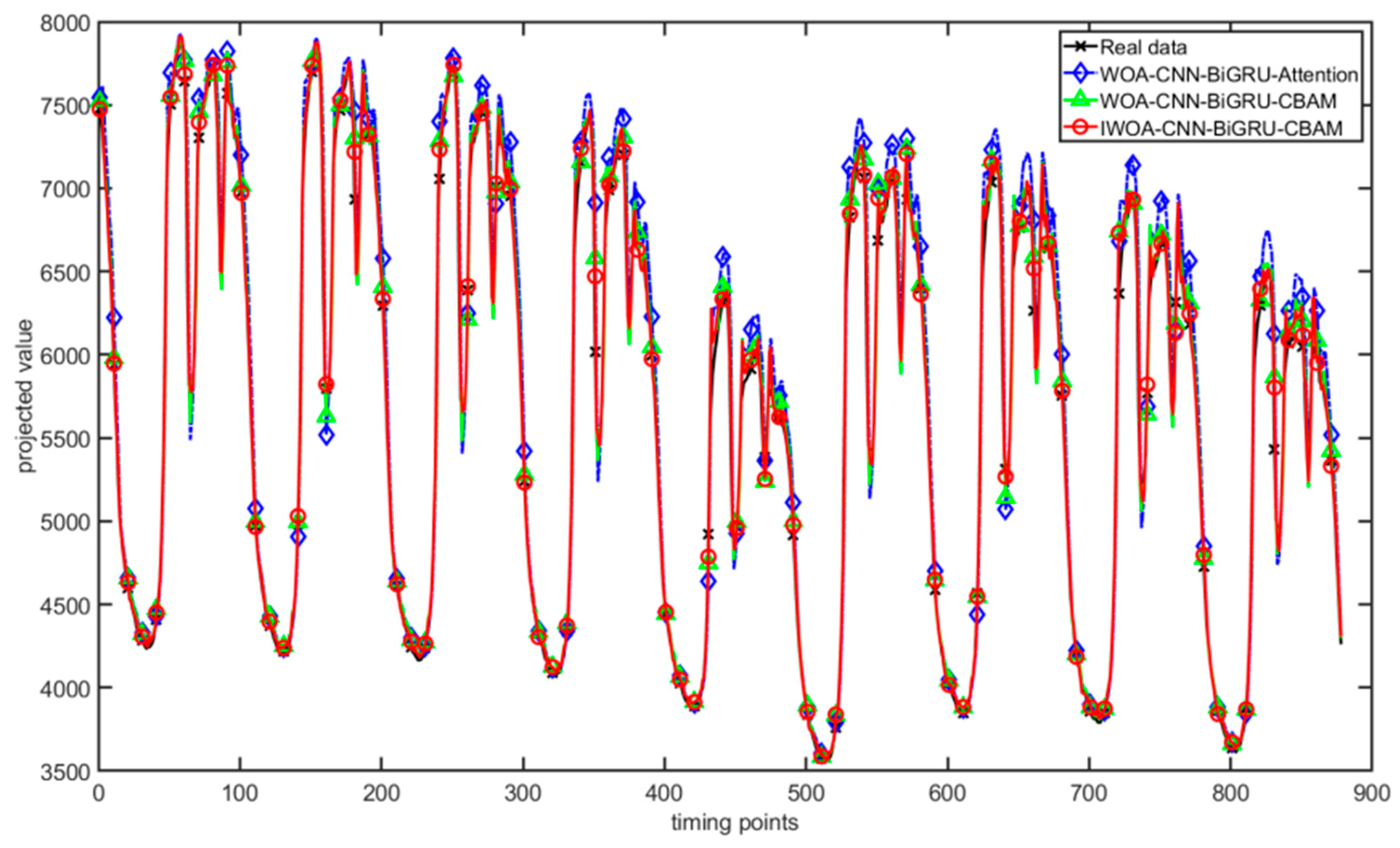
The IWOA-CNN-BiGRU-CBAM is compared with WOA-CNN-BiGRU-Attention and WOA-CNN-BiGRU-CBAM on the dataset for the experiments. In this case, the hyperparameters for optimization are all chosen as the learning rate of the model; the BiGRU layer’s hidden neurons count with L2 regularization coefficients, the number of algorithmic search agents are all 6, and the number of iterations is 10. Each parameter of the model is detailed in Table 1. In addition, Figure 11 shows the loss training plot of the IWOA-CNN-BiGRU-CBAM model. Figure 12 shows a comparison plot of the predictions of the three models.

Table 2. An analysis of the accuracy of forecasting in several models.

Model	RMSE/kw	Var	R2	MAE$/\mathbf{kw}$	Var
WOA-CNN-BiGRU-Attention	119.5528	83.5879	0.99099	94.8737	81.6412
WOA-CNN-BiGRU-CBAM	105.008	61.5237	0.99305	81.9422	65.8345
IWOA-CNN-BiGRU-CBAM	86.4299	25.4416	0.99529	56.0482	21.5276

illustrates the prediction accuracy results of these three models. All the above results are average results obtained from 50 model runs. The variance of the results of these 50 runs is recorded in Table 2.

As shown in Figure 12 and Table 2 comparing WOA-CNN-BiGRU-CBAM and WOA-CNN-BiGRU-Attention, there is a 14.5448 and 12.9315 decrease in the RMSE and MAE, respectively, and a 0.00206 improvement in R², indicating that adding CBAM can enhance the accuracy of predictions and fitting effect of the model; then, comparing IWOA-CNN-BiGRU-CBAM and WOA-CNN-BiGRU-CBAM, RMSE and MAE are reduced by 18.5781 and 25.8940, respectively, and R² is improved by 0.00224, suggesting that the IWOA improvement effect is superior to that of WOA. In conclusion, the prediction accuracy and fitting effect of the IWOA-CNN-BiGRU-CBAM model established in this study are excellent. Meanwhile, by comparing the variance of RMSE and MAE of the above three models, the stability of the IWOA-CNN-BiGRU-CBAM model is shown to be superior.

4.3. Validation of IWOA

The performance evaluation of the five algorithms presented in this paper is conducted using the cec2022 test function set. IWOA and WOA, msWOA [42], mFOA [43], mPSO [44], and mSCA [45] are compared in this test function set, and these algorithms are run 100 times, respectively. The worst, best, and mean values and the standard deviation are taken as the evaluation indexes, and

Table 3. The comparison of obtained solutions.

(a) F1–F6
Function		IWOA	WOA	msWOA	mFOA	mPSO	mSCA
F1	best	300	300	300	300	300.0001	300.0001
	worst	300	300	300.0294	300	300.3384	300.0524
	mean	300	300	300.0035	300	300.0486	300.0133
	std	2.27 × 10−12	7.54 × 10−8	0.004477	0	0.058025	0.0128
F2	best	400.2777	401.6992	413.2647	403.3437	408.3338	421.0018
	worst	479.3967	717.1292	1183.94	748.6179	857.7683	502.4041
	mean	422.1213	458.1891	612.9995	475.8902	496.6692	455.5791
	std	24.36634	61.39288	171.0077	73.62923	103.6627	16.61971
F3	best	600	600	600.0087	600	600.0081	600.0409
	worst	600.003	600.1573	600.9438	600.0976	600.855	601.2707
	mean	600.0001	600.0202	600.2592	600.0023	600.2633	600.4247
	std	0.000322	0.037195	0.171672	0.011841	0.173438	0.238818
F4	best	812.9351	812.3129	812.4637	809.7649	820.047	822.6616
	worst	876.6685	900.7113	868.3376	853.5478	863.1018	853.6567
	mean	843.9564	838.2078	839.1272	825.2598	838.2995	839.0441
	std	20.24485	14.55806	12.25264	9.418728	7.613952	6.627878
F5	best	900	900	900	900	900	900
	worst	900	900	900.0076	900	900.0735	900.0028
	mean	900	900	900.0006	900	900.0067	900.0004
	std	1.37 × 10−11	1.81 × 10−7	0.001221	0	0.009845	0.000393
F6	best	1883.559	1891.493	6177.15	1842.683	15,077.6	41,854.58
	worst	8135.544	42,432.68	530,264.3	2,982,948	1,494,901	10,471,639
	mean	3500.321	4691.582	110,153.8	81,266.17	446,976.4	1,507,792
	std	1631.162	4312.319	99,805.16	365,816	346,708	1,588,267
(b) F7–F12
Function		IWOA	WOA	msWOA	mFOA	mPSO	mSCA
F7	best	2089.897	2077.67	2103.471	2075.351	2073.808	2105.105
	worst	2384.001	2482.748	2338.527	2348.3	2292.895	2240.146
	mean	2204.2	2214.59	2187.575	2178.615	2160.963	2164.61
	std	63.97263	70.09778	48.44177	57.09852	45.1093	24.47191
F8	best	2208.254	2222.903	2230.031	2218.175	2221.917	2220.173
	worst	2247.829	2285.338	2374.429	2257.819	2414.043	2239.526
	mean	2232.685	2236.215	2261.016	2230.435	2242.665	2232.556
	std	5.452965	11.42288	46.94911	6.241747	28.48983	3.501958
F9	best	2300	2300	2300.055	2300	2300.342	2300.031
	worst	2500	2300.031	2500.089	2500.304	2306.865	2303.564
	mean	2304	2300.006	2323.26	2351.198	2302.544	2301.311
	std	28.14106	0.006375	62.57088	84.78268	1.550569	0.760773
F10	best	2500.174	2500.291	2500.566	2500.385	2500.862	2500.655
	worst	2501.906	3740.123	2502.508	2669.412	3943.525	2649.952
	mean	2500.704	2600.032	2501.291	2540.491	2607.37	2511.309
	std	0.252649	227.4614	0.418806	63.03421	231.2993	36.14797
F11	best	2600.182	2625.687	2735.615	3010.665	2775.496	2758.747
	worst	4654.493	4679.533	4620.619	11652.84	3780.67	2883.853
	mean	2940.107	2986.62	3154.811	5540.764	3101.457	2785.171
	std	327.2382	270.581	275.6916	1545.086	328.7328	19.76031
F12	best	2861.531	2864.334	2896.135	2860.835	2862.535	2864.759
	worst	2887.873	3094.582	2961.506	3070.876	3043.66	2879.305
	mean	2867.674	2902.119	2952.313	2902.824	2892.679	2870.294
	std	4.905309	43.53633	5.842151	38.01212	32.24627	2.236951

depicts the results. Further, the overall results were subjected to the Friedman test [46], and the results are shown in Table 3, where the functions F1, F3, F5, and F9 were tested with dimension 2. The functions F2, F4, F6, F10, F11, F12 were tested with dimension 10, and the functions F7, F8 were tested with dimension 20. Figure 13 displays the convergence curves of each algorithm for the F2, F3, F8, and F12 functions.

As shown in Table 3, when IWOA optimizes the F1, F2, F3, F5, F6, F8, F9, F10, and F12 functions, its optimal value is closest to the theoretically optimal value, the mean value index is the best among many algorithms, and the standard deviation index is smaller, indicating that its optimization effect is more stable and the algorithm performance is better; to further assess the strengths and weaknesses of the algorithms, the results in the table are subjected to non-parametric tests. The results are displayed in

Table 4. Comparison of different algorithmic rank averages.

Algorithm	Ordinal Mean
IWOA	2.87
WOA	4.15
msWOA	5.77
mFOA	3.98
mPSO	5.97
mSCA	4.15

. The IWOA has been determined to have the highest ranking, and its optimization effect is notably outstanding.

Figure 13 proves that IWOA performs better in optimizing the F2, F3, F8, and F12 functions. Initially, these functions display more fluctuations but converge rapidly in the early phases. The fluctuations decrease when the iterations continue to progress, and the downward trend of the curve indicates that the search agents are effectively collaborating to update their positions to achieve better results. Table 3 and Table 4 provide evidence that IWOA exhibits superior convergence behaviour and displays an improved capacity to balance the two extremes of exploitation and exploration throughout the iteration process compared to other algorithms.

4.4. Comparative Experiments

In this section, all the model parameters involved are depicted in Table 1, with the average results obtained from 50 runs of the model.

Firstly, the hidden neuron number in the BiGRU layer, the learning rate, the L2 regularization coefficients, the number of searching agents (fixed at six), and the number of iterations (maintained at ten) are optimized by the IWOA algorithm for the CNN-BiGRU, CNN-BiGRU-Attention, and CNN-BiGRU-CBAM models, respectively. The mentioned models are employed for the experiments on the selected dataset, and the forecasts’ accuracy findings are illustrated in

Table 5. Comparison of forecasting accuracy in different models.

Model	RMSE/kw	R2	MAE$/\mathbf{kw}$
IWOA-BiGRU	183.9619	0.9789	124.1239
IWOA-CNN-BiGRU	158.6322	0.98431	115.6731
IWOA-CNN-BiGRU-Attention	111.2914	0.99225	85.4261
IWOA-CNN-BiGRU-CBAM	86.4299	0.99529	56.0482

.

In Table 5, by introducing CNN, the prediction error RMSE is reduced by 13.77%, MAE is reduced by 6.81%, and R² is improved by 0.00541. By introducing the attention mechanism, the prediction error RMSE is reduced from 158.6322 to 111.2914, which is a reduction of 29.84%; MAE is reduced by 26.15%, and R² is improved by 0.00794, which is more than that of introducing CNN. Therefore, the effect of the attention mechanism on the performance of the model’s predictions is truly astounding. While introducing CBAM instead of SE, the prediction error RMSE is reduced by 22.34%, MAE by 34.39%, and R² is improved by 0.00304, proving the superiority of CBAM.

Then, five algorithms such as WOA, msWOA, mFOA, mPSO, and mSCA, are optimized for, respectively, hidden neuron count in the BiGRU layer, learning rate, and L2 regularization coefficients of the CNN-BiGRU-CBAM model; this model optimized with IWOA was used for experiments on the selected dataset.

Table 6. Comparative analysis of forecast precision across various models.

Model	RMSE/kw	R2	MAE$/\mathbf{kw}$
IWOA-CNN-BiGRU-CBAM	86.4299	0.99529	56.0482
WOA-CNN-BiGRU-CBAM	105.008	0.99305	81.9422
msWOA-CNN-BiGRU-CBAM	101.7268	0.99348	77.2248
mFOA-CNN-BiGRU-CBAM	300.6814	0.94303	239.2391
mPSO-CNN-BiGRU-CBAM	116.3347	0.99147	88.6592
mSCA-CNN-BiGRU-CBAM	102.1971	0.99342	69.5965

illustrates the load-forecasting accuracy of various modelling approaches presented.

According to Table 6, the proposed model demonstrates the least amount of prediction error when contrasted with the other five models. Its RMSE value is 86.4299, R² value is 0.99529, and MAE value is 56.0482, which are improved by 18.5781, 0.00224, and 25.894, respectively, compared to WOA, which shows that the influence of IWOA on optimization is mainly reflected in the significant reduction of RMSE and MAE. Comparing it with msWOA, the effectiveness of the improvement measures presented in this research for WOA is evident. Then, the predictive accuracy of the optimized model of iWOA is paired against that of the three improved algorithms, namely mFOA, mPSO, and mSCA. It can be seen that the optimized model of IWOA has a considerable decrease in RMSE and MAE, and the precision of the prediction is greatly enhanced. Meanwhile, the improvement of R² also indicates that the model-fitting effect of the optimized model of IWOA has been improved. Simultaneously, the enhancement of the indicators also signifies that the model-fitting effect of the IWOA optimization presented in this paper has been enhanced. To summarize, the model proposed exhibits enhancements in the indicators RMSE, MAE, R², indicating that the overall prediction accuracy and model performance of the IWOA-CNN-BIGRU-CBAM model proposed has been greatly improved in the prediction process. The efficacy of the model described in this research is validated.

Then, the predictions of BiLSTM, IWOA-CNN-BiLSTM-Attention, IWOA-CNN-BiLSTM-CBAM, and IWOA-CNN-BiGRU-CBAM models are compared with each other, and

Table 7. Comparison of forecasting accuracy in different models.

Model	RMSE/kw	R2	MAE$/\mathbf{kw}$
BiLSTM	387.3769	0.92588	276.0312
IWOA-CNN-BiLSTM-Attention	185.1584	0.96124	162.2335
IWOA-CNN-BiLSTM-CBAM	154.6835	0.97247	137.2238
IWOA-CNN-BiGRU-CBAM	86.4299	0.99529	56.0482

depicts the corresponding results.

In Table 7, comparing IWOA-CNN-BiLSTM-Attention with BiLSTM, RMSE, MAE, respectively, are reduced by 202.2185 and 113.7977, and R² improves by 0.03536. Comparing IWOA-CNN-BiLSTM-CBAM with IWOA-CNN-BiLSTM-Attention, RMSE, MAE, respectively, are reduced by 30.4749, 25.0097, and R² improves by 0.01123. Comparing IWOA-CNN-BiGRU-CBAM with IWOA-CNN-BiLSTM-CBAM, RMSE and MAE decrease, respectively, by 68.2536, 81.1756, and R² improves by 0.02282. As seen from the above, the proposed IWOA-CNN-BiGRU-CBAM model is more efficient in optimisation than BiLSTM and other models.

5. Conclusions

An IWOA-CNN-BiGRU-CBAM model is proposed to resolve the challenge of short-term power load forecasting. To address the issue of the SE attention mechanism’s inability to effectively capture information in the spatial dimension and its limited applicability to scenarios with many channels, the CBAM is proposed as a replacement. Meanwhile, considering the drawbacks of WOA falling into local optimal solutions and the strong dependence on the initial solution, an improved WOA algorithm is proposed and subsequently employed for hyper-parameter training of CNN-BiGRU-CBAM to enhance the precision of model training. The proposed IWOA-CNN-BiGRU-CBAM model is applied to the power load dataset for short-term forecasting. The experiment’s results indicate that the CBAM, as presented, can significantly enhance the model’s potential for generalization. The suggested IWOA exhibits enhanced optimization search capabilities and is better suited for addressing the hyperparameter optimization problem of the CNN-BIGRU-CBAM model. Compared with other models, IWOA-CNN-BiGRU-CBAM improves the R² metric by 0.0224, RMSE decreases by 18.5781, and MAE decreases by 25.8940. The prediction accuracy and the interval coverage of the IWOA-CNN-BiGRU-CBAM model proposed are higher on the dataset, indicating a superior generalization capacity. The next step involves enhancing the multi-scenario processing capability of the forecasting model by incorporating meteorological factors such as rainfall, temperature, humidity, and holidays when addressing the more sophisticated task of short-term load forecasting in complex settings.

References

1. Sheng, Z.; An, Z.; Wang, H.; Chen, G.; Tian, K. Residual LSTM based short-term load forecasting. Appl. Soft Comput. J. 2023, 144, 110461. [Google Scholar] [CrossRef]
2. Anh, N.N.; Dat, D.T.; Elena, V.; Vijender, K.S. Short-term forecasting electricity load by long short-term memory and reinforcement learning for optimization of hyper-parameters. Evol. Intell. 2023, 16, 1729–1746. [Google Scholar]
3. Kim, D.; Lee, D.; Nam, H.; Joo, S.K. Short-Term Load Forecasting for Commercial Building Using Convolutional Neural Network (CNN) and Long Short-Term Memory (LSTM) Network with Similar Day Selection Model. J. Electr. Eng. Technol. 2023, 18, 4001–4009. [Google Scholar] [CrossRef]
4. Dima, A.; Mark, L. Short-term load forecasting in smart meters with sliding window-based ARIMA algorithms. Vietnam J. Comput. Sci. 2018, 5, 241–249. [Google Scholar]
5. Mi, J.; Fan, L.; Duan, X.; Qiu, Y. Short-Term Power Load Forecasting Method Based on Improved Exponential Smoothing Grey Model. Math. Probl. Eng. 2018, 2018, 3894723. [Google Scholar] [CrossRef]
6. Shalini, S.; Angshul, M.; Victor, E.; Emilie, C. Blind Kalman Filtering for Short-Term Load Forecasting. IEEE Trans. Power Syst. 2020, 35, 4916–4919. [Google Scholar]
7. Pang, X.; Sun, W.; Li, H.; Wang, Y.; Luan, C. Short-term power load forecasting based on gray relational analysis and support vector machine optimized by artificial bee colony algorithm. Peer J. Comput. Sci. 2022, 8, e1108. [Google Scholar] [CrossRef] [PubMed]
8. Jin, Y.; Guo, H.; Wang, J.; Song, A. A Hybrid System Based on LSTM for Short-Term Power Load Forecasting. Energies 2020, 13, 6241. [Google Scholar] [CrossRef]
9. Zhao, H.; Zhou, Z.; Zhang, P. Forecasting of the Short-Term Electricity Load Based on WOA-BILSTM. Int. J. Pattern Recognit. Artif. Intell. 2023, 37, 272–286. [Google Scholar] [CrossRef]
10. Gao, X.; Li, X.; Zhao, B.; Ji, W.; Jing, X.; He, Y. Short-Term Electricity Load Forecasting Model Based on EMD-GRU with Feature Selection. Energies 2019, 12, 1140. [Google Scholar] [CrossRef]
11. Ji, X.; Liu, D.; Xiong, P. Multi-model fusion short-term power load forecasting based on improved WOA optimization. Math. Biosci. Eng. 2022, 19, 13399–13420. [Google Scholar] [CrossRef] [PubMed]
12. Chu, Z.; Tian, P.; Shahzad, N.M. A novel integrated photovoltaic power forecasting model based on variational mode decomposition and CNN-BiGRU considering meteorological variables. Electr. Power Syst. Res. 2022, 213, 108796. [Google Scholar]
13. Dao, F.; Zeng, Y.; Qian, J. Fault diagnosis of hydro-turbine via the incorporation of bayesian algorithm optimized CNN-LSTM neural network. Energy 2024, 290, 2901–2916. [Google Scholar] [CrossRef]
14. Li, D.; Wang, X.; Sun, J.; Feng, Y. Radial Basis Function Neural Network Model for Dissolved Oxygen Concentration Prediction Based on an Enhanced Clustering Algorithm and Adam. IEEE Access 2021, 9, 44521–44533. [Google Scholar] [CrossRef]
15. Ge, L.; Xian, Y.; Wang, Z.; Gao, B.; Chi, F.; Sun, K. A GWO-GRNN based model for short-term load forecasting of regional distribution network. CSEE J. Power Energy Syst. 2020, 7, 1093–1101. [Google Scholar]
16. Mirjalili, S.; Lewis, A. The Whale Optimization Algorithm. Adv. Eng. Softw. 2016, 95, 51–67. [Google Scholar] [CrossRef]
17. Wu, F.; Cattani, C.; Song, W.; Zio, E. Fractional ARIMA with an improved cuckoo search optimization for the efficient Short-term power load forecasting. Alex. Eng. J. 2020, 59, 3111–3118. [Google Scholar] [CrossRef]
18. Bahrami, S.; Hooshmand, R.-A.; Parastegari, M. Short term electric load forecasting by wavelet transform and grey model improved by PSO (particle swarm optimization) algorithm. Energy 2014, 72, 434–442. [Google Scholar] [CrossRef]
19. Abu-Shikhah, N.; Elkarmi, F.; Aloquili, O.M. Medium-Term Electric Load Forecasting Using Multivariable Linear and Non-Linear Regression. Smart Grid Renew. Energy 2011, 2, 126–135. [Google Scholar] [CrossRef]
20. Zhang, X.; Wang, J.; Zhang, K. Short-term electric load forecasting based on singular spectrum analysis and support vector machine optimized by Cuckoo search algorithm. Electr. Power Syst. Res. 2017, 146, 270–285. [Google Scholar] [CrossRef]
21. Liu, T.; Fan, D.; Chen, Y.; Dai, Y.; Jiao, Y.; Cui, P.; Wang, Y.; Zhu, Z. Prediction of CO2 solubility in ionic liquids via convolutional autoencoder based on molecular structure encoding. AIChE J. 2023, 69, e18182. [Google Scholar] [CrossRef]
22. Fan, D.; Xue, K.; Zhang, R.; Zhu, W.; Zhang, H.; Qi, J.; Zhu, Z.; Wang, Y.; Cui, P. Application of interpretable machine learning models to improve the prediction performance of ionic liquids toxicity. Sci. Total Environ. 2023, 908, 168168. [Google Scholar] [CrossRef] [PubMed]
23. Bian, H.; Zhong, Y.; Sun, J.; Shi, F. Study on power consumption load forecast based on K-means clustering and FCM–BP model. Energy Rep. 2020, 6, 693–700. [Google Scholar] [CrossRef]
24. Lin, W.; Zhang, B.; Li, H.; Lu, R. Short-term load forecasting based on EEMD-Adaboost-BP. Syst. Sci. Control Eng. 2022, 10, 846–853. [Google Scholar] [CrossRef]
25. Liu, T.; Chu, X.; Fan, D.; Ma, Z.; Dai, Y.; Zhu, Z.; Wang, Y.; Gao, J. Intelligent prediction model of ammonia solubility in designable green solvents based on microstructure group contribution. Mol. Phys. 2022, 120, e2124203. [Google Scholar] [CrossRef]
26. Mu, Y.; Wang, M.; Zheng, X.; Gao, H. An improved LSTM-Seq2Seq-based forecasting method for electricity load. Front. Energy Res. 2023, 10, 1093667. [Google Scholar] [CrossRef]
27. Liu, F.; Liang, C. Short-term power load forecasting based on AC-BiLSTM model. Energy Rep. 2024, 11, 1570–1579. [Google Scholar] [CrossRef]
28. Wu, K.; Wu, J.; Feng, L.; Yang, B.; Liang, R.; Yang, S.; Zhao, R. An attention-based CNN-LSTM-BiLSTM model for short-term electric load forecasting in integrated energy system. Int. Trans. Electr. Energy Syst. 2020, 31, 576–583. [Google Scholar] [CrossRef]
29. Jia, T.; Yao, L.; Yang, G.; He, Q. A Short-Term Power Load Forecasting Method of Based on the CEEMDAN-MVO-GRU. Sustainability 2022, 14, 16460. [Google Scholar] [CrossRef]
30. Liang, R.; Chang, X.; Jia, P.; Xu, C. Mine Gas Concentration Forecasting Model Based on an Optimized BiGRU Network. ACS Omega 2020, 5, 28579–28586. [Google Scholar] [CrossRef]
31. Meng, Y.; Chang, C.; Huo, J.; Zhang, Y.; Al-Neshmi, H.M.M.; Xu, J.; Xie, T. Research on Ultra-Short-Term Prediction Model of Wind Power Based on Attention Mechanism and CNN-BiGRU Combined. Front. Energy Res. 2022, 10, 920835. [Google Scholar] [CrossRef]
32. Xu, Y.; Jiang, X. Short-term power load forecasting based on BiGRU-Attention-SENet model. Energy Sources Part A Recovery Util. Environ. Eff. 2022, 44, 973–985. [Google Scholar] [CrossRef]
33. Yang, B.; Wang, Y.; Zhan, Y. Lithium Battery State-of-Charge Estimation Based on a Bayesian Optimization Bidirectional Long Short-Term Memory Neural Network. Energies 2022, 15, 4670. [Google Scholar] [CrossRef]
34. Feng, M.; Duan, Y.; Wang, X.; Zhang, J.; Ma, L. Carbon price prediction based on decomposition technique and extreme gradient boosting optimized by the grey wolf optimizer algorithm. Sci. Rep. 2023, 13, 18447. [Google Scholar] [CrossRef] [PubMed]
35. Guo, J.; Chen, C.; Wen, H.; Cai, G.; Liu, Y. Prediction model of goaf coal temperature based on PSO-GRU deep neural network. Case Stud. Therm. Eng. 2024, 53, 103813. [Google Scholar] [CrossRef]
36. Xiao, M.; Luo, R.; Chen, Y.; Ge, X. Prediction model of asphalt pavement functional and structural performance using PSO-BPNN algorithm. Constr. Build. Mater. 2023, 407, 133534. [Google Scholar] [CrossRef]
37. Luo, J.; Gong, Y. Air pollutant prediction based on ARIMA-WOA-LSTM model. Atmos. Pollut. Res. 2023, 14, 101761. [Google Scholar] [CrossRef]
38. Sun, Y.; Zhang, J.; Yu, Z.; Liu, Z.; Yin, P. WOA (Whale Optimization Algorithm) Optimizes Elman Neural Network Model to Predict Porosity Value in Well Logging Curve. Energies 2022, 15, 4456. [Google Scholar] [CrossRef]
39. Chen, L.; Li, S.; Bai, Q.; Yang, J.; Jiang, S.; Miao, Y. Review of Image Classification Algorithms Based on Convolutional Neural Networks. Remote Sens. 2021, 13, 4712. [Google Scholar] [CrossRef]
40. Mansour, A.A.; Tilioua, A.; Touzani, M. Bi-LSTM, GRU and 1D-CNN models for short-term photovoltaic panel efficiency forecasting case amorphous silicon grid-connected PV system. Results Eng. 2024, 21, 101886. [Google Scholar] [CrossRef]
41. Woo, S.; Park, J.; Lee, J.-Y.; Kweon, I.S. CBAM: Convolutional Block Attention Module; Lecture Notes in Computer Science (Including Subseries Lecture Notes in Artificial Intelligence and Lecture Notes in Bioinformatics); Springer: Cham, Switzerland, 2018; Volume 11211, pp. 3–19. [Google Scholar]
42. Yang, W.; Xia, K.; Fan, S.; Wang, L.; Li, T.; Zhang, J.; Feng, Y. A Multi-Strategy Whale Optimization Algorithm and Its Application. Eng. Appl. Artif. Intell. 2022, 108, 104558. [Google Scholar] [CrossRef]
43. Mirjalili, S. Moth-flame optimization algorithm: A novel nature-inspired heuristic paradigm. Knowl.-Based Syst. 2015, 89, 228–249. [Google Scholar] [CrossRef]
44. Zhou, H.; Pang, J.; Chen, P.-K.; Chou, F.-D. A modified particle swarm optimization algorithm for a batch-processing machine scheduling problem with arbitrary release times and non-identical job sizes. Comput. Ind. Eng. 2018, 123, 67–81. [Google Scholar] [CrossRef]
45. Gupta, S.; Deep, K. A hybrid self-adaptive sine cosine algorithm with opposition based learning. Expert Syst. Appl. 2019, 119, 210–230. [Google Scholar] [CrossRef]
46. Derrac, J.; García, S.; Molina, D.; Herrera, F. A practical tutorial on the use of nonparametric statistical tests as a methodology for comparing evolutionary and swarm intelligence algorithms. Swarm Evol. Comput. 2011, 1, 3–18. [Google Scholar] [CrossRef]
Figure 1. Structure of CNN-BiGRU-CBAM.
Energies 17 02559 g001
Figure 2. Structure of CNN.
Energies 17 02559 g002
Figure 3. Structure of GRU.
Energies 17 02559 g003
Figure 4. Structure of BiGRU.
Energies 17 02559 g004
Figure 5. CBAM architecture.
Energies 17 02559 g005
Figure 6. Channel attention structure.
Energies 17 02559 g006
Figure 7. Spatial attention structure.
Energies 17 02559 g007
Figure 8. Good point set method-generated initial two-dimensional population.
Energies 17 02559 g008
Figure 9. Initial two-dimensional population generated using the stochastic method.
Energies 17 02559 g009
Figure 10. Flowchart of the IWOA.
Energies 17 02559 g010
Figure 11. Training loss of the proposed model.
Energies 17 02559 g011
Figure 12. Comparison of forecasting results.
Energies 17 02559 g012
Figure 13. Convergence diagram.
Energies 17 02559 g013