Research on the EMA Control Method Based on Transmission Error Compensation

Abstract

This research investigates the impact of nonlinear clearance factors on position tracking accuracy in the servo drive system of a harmonic reducer. The study introduces a technique for modeling and compensating for transmission errors, thereby improving position tracking accuracy through online compensation combined with an auto-disturbance rejection controller. Initially, the mathematical model of the permanent magnet synchronous motor is outlined, and the current loop and speed loop control models are derived. Subsequently, an electromechanical actuator (EMA) simulation model with clearance is established, and detailed simulation analysis is conducted to verify the impact of clearance on tracking accuracy. A model for online compensation of transmission errors is then developed. Following the principles of active disturbance rejection control (ADRC), a second-order ADRC is formulated for real-time compensation of transmission errors in EMA position mode. Finally, through no-load and load experiments, the change in position tracking error with and without transmission error compensation is compared and analyzed. The results demonstrate that utilizing automatic disturbance rejection control with transmission error compensation achieves the highest position tracking accuracy. Compared to the proportion integration differentiation (PID) control method, the root mean square of position tracking error is reduced by approximately 12.8% and 17.3% under no-load and load conditions, respectively. By compensating for position errors online, the accuracy of the EMA position can be improved.

1. Introduction

Robot joints, also known as electromechanical actuators (EMAs), play a critical role in the effectiveness of robots overall [1,2]. As humanoid and service robots advance rapidly, EMAs are evolving to become more compact, lightweight, modular, integrated, precise, and dynamically efficient. Typically, EMAs consist of motors, reducers, encoders, drivers, and controllers. Harmonic drives are particularly notable for their characteristics like low noise, compact size, lightweight, high load capacity, high reduction ratio, and efficiency, making them increasingly popular in industrial, service, and specialized robots. The accuracy of harmonic drives’ transmission is influenced by factors such as transmission friction, stiffness, and clearance [3,4,5,6]. This paper focuses on examining how clearance affects transmission accuracy, considering causes like meshing gaps between flexible and rigid wheels, manufacturing and assembly inaccuracies, clearance in moving parts of wave generators, elastic deformation, and temperature variations. Clearance significantly impacts EMA’s operational precision, leading to oscillations near steady state, “impact phenomenon” during start, stop, acceleration, and deceleration phases, and “flat top phenomenon” in the sine tracking of position loops, ultimately reducing the dynamic tracking accuracy. Additionally, as wear and tear accumulate over service time, gaps widen, further influencing EMA performance.

Enhancing the precision of machining and assembly in harmonic drives can reduce gaps, but this method is expensive and poses challenges for widespread use, with limited effectiveness in gap reduction [7]. Compensation control, achieved through controllers such as sliding mode and neural network compensation control, often tackles external disturbances caused by gap effects without direct measurement for compensation. The field-oriented control algorithm and proportion integration differentiation (PID) triple closed-loop control strategy are commonly used in EMA control systems. Despite the simplicity, easy implementation, and minimal control parameters of the PID controller, its selection of error signal can introduce significant initial system errors, potentially leading to overshoot. Differential signal approximation amplifies noise, significantly distorting the signal. Balancing speed and overshoot remains a challenge through linear combinations of proportional, integral, and differential actions. Han Jingqing introduced active disturbance rejection control technology, which, unlike traditional methods, does not rely on the precise mathematical model of the controlled object [8]. It considers uncertain, unmodeled parts of the system, external disturbances, complex nonlinearities, and time-varying factors such as “total disturbance”. An extended state observer estimates this disturbance in real time for feedback control compensation, enhancing dynamic performance through nonlinear feedback and managing nonlinear and uncertain system elements [9,10]. Active disturbance rejection controllers have been utilized in motor control systems by various scholars, notably improving motor control performance [11,12,13,14].

Further research examined the first-order active disturbance rejection control (ADRC) for speed and current loops, resulting in the development of a cascade active disturbance rejection controller for the PMSM speed control system [15]. The control law consisting of proportional feedback and disturbance feedforward compensation is developed to control the q-axis current, but the application of this method is relatively cumbersome. Integrating a sliding mode controller into ADRC decreased steady-state errors in the permanent magnet synchronous motor control system [16]. However, this method has a slight vibration problem. A first-order speed loop ADRC can enhance PMSM speed regulation; however, its accuracy heavily relies on the extended state observer’s observation accuracy [17,18]. Simulation of the PMSM model and FOC algorithm utilized first-order ADRC instead of the d-q axis PI controller to enhance the dynamic and static performance of the permanent magnet synchronous motor [19]. This method introduces two ADRC controllers, increasing the difficulty of adjusting control parameters.

This article presents a nonlinear mathematical model for the transmission clearance of EMAs and verifies the effect of different clearance values on tracking accuracy through simulation. Following this, a model for compensating position errors was developed and integrated into the Active ADRC algorithm to improve the control precision of EMAs by compensating for position errors. The methodology was validated through experiments.

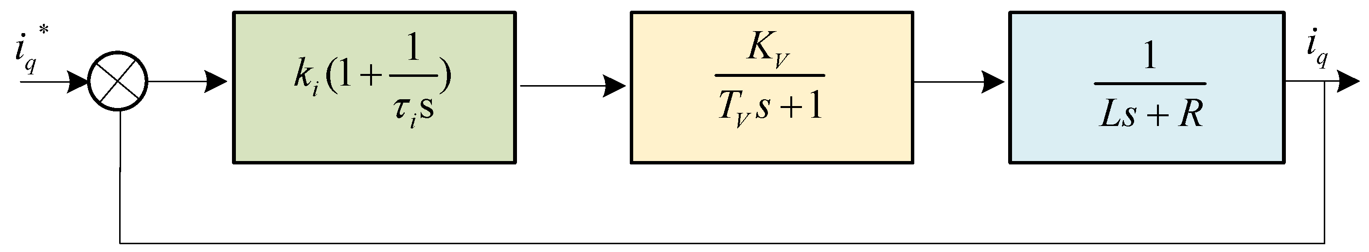
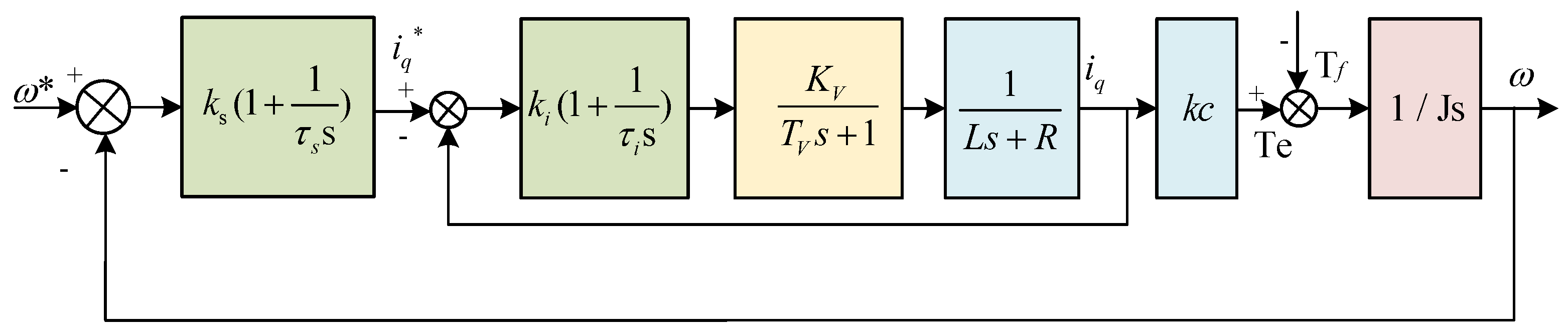
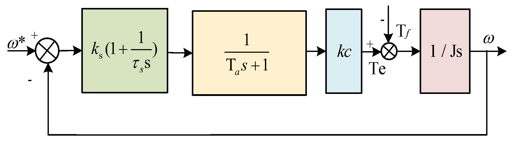
2. The PMSM Mathematical Model in the EMA

PMSMs have the advantages of simple structure, high power density, high efficiency, and PMSMs offer the advantages of a simple structure, high power density, high efficiency, and rapid dynamic response, making them extensively utilized in various fields such as robotics, aerospace, precision instruments, machine tools, new energy vehicles, and healthcare [20,21,22,23,24]. The mathematical model of EMAs primarily encompasses two nonlinear factors: PMSM and harmonic drive. The coupling between PMSM and harmonic drive occurs through the torque current. Vector control (VC), also referred to as field-oriented control (FOC) and direct torque control (DTC), is a common approach in PMSMs. While FOC offers high performance, it involves complex calculations compared to DTC control. The PMSM mathematical model under the FOC control strategy mainly comprises a voltage equation, magnetic linkage equation, electromagnetic torque equation, and mechanical equation. According to references [25,26], the mathematical model of the PMSM in a two-phase d-q rotating coordinate system is

$$\left\{\begin{array}{l}\left.\begin{array}{l}{u}_d=R_s{i}_d+\frac{d{\Psi }_d}{dt}-\omega {\Psi }_q\hspace{1em}\hspace{1em}\hspace{1em}\hspace{1em}\\ u_q=R_s{i}_q+\frac{d{\Psi }_q}{dt}+\omega {\Psi }_d\hspace{1em}\hspace{1em}\hspace{1em}\hspace{1em}\end{array}\right\}\mathrm{Voltage} \mathrm{equation}\\ \left.\begin{array}{l}{\Psi }_d=L_d{i}_d+{\Psi }_f\hspace{1em}\hspace{1em}\hspace{1em}\hspace{1em}\hspace{1em}\hspace{1em}\hspace{1em}\\ {\Psi }_q=L_q{i}_q\hspace{1em}\hspace{1em}\hspace{1em}\hspace{1em}\hspace{1em}\hspace{1em}\hspace{1em}\end{array}\right\}\mathrm{Flux} \mathrm{equation}\\ \left.T_e=1.5p_n[{\Psi }_f{i}_q+(L_d-L_q)i_d{i}_q]\hspace{1em}\right\}\mathrm{Electromagnetic} \mathrm{torque} \mathrm{equation}\\ \left.J\frac{d{\omega }_r}{dt}=T_e-T_L-B{\omega }_r\hspace{1em}\hspace{1em}\hspace{1em}\hspace{1em}\hspace{1em}\right\}\mathrm{Mechanical} \mathrm{equation}\end{array}\right.$$

(1)

where, u_d and u_q represent the stator voltage in the d-q coordinate system, ω_e is the electrical angular velocity, i_d and i_q denote the stator current in the d-q coordinate system, R_s is the phase resistance, and ψ_d and ψ_q represent the d-q axis excitation winding flux. The expressions for ψ_d and ψ_q are the magnetic flux equations in Equation (1).

i_d, i_q, u_d, u_q, L_d, L_q, ψ_d, and ψ_q are the d-q axis current, voltage, inductance, and flux, respectively; p_n is the polar logarithm; T_e is the electromagnetic torque; J is the moment of inertia; T_L is the load torque; and B is the damping coefficient. ψ_f is the permanent magnet flux, and ω and ω_r are the electrical angular velocity and mechanical angular velocity, respectively. For a surface-mounted PMSM with L_d = L_q = L_s, using a surface-mounted PMSM or the i_d=0 control method, the electromagnetic torque equation in Equation (1) can be simplified as

$$T_e=1.5p_n{\Psi }_f{i}_q$$

(2)

The current loop is at the core of the PMSM’s three closed-loop control system, playing a pivotal role in ensuring the system’s precision and dynamic properties [27,28]. Essentially, it consists of a PI controller circuit, an inverter circuit, and an armature circuit. As changes in motor speed characteristics are much smaller than changes in electrical characteristics, the influence of back electromotive force on the current loop is neglected. Figure 1 illustrates the equivalent control block diagram for the current loop.

According to Figure 1, the open-loop transfer function of the PMSM is

$$G_{\mathrm{k}s}(s)=k_i(\frac{{\tau }_i\mathrm{s}+1}{{\tau }_i\mathrm{s}})\ast \frac{K_V}{T_{V}s+1}\ast \frac{1}{Ls+R}$$

(3)

Let T_i = L/R, T_i is the PMSM electromagnetic time constant, and let τ_i = T_i; Equation (3) can be simplified.

$$G_{ks}(s)=\frac{k_i{K}_V/R}{{\tau }_{i}s(T_{V}s+1)}$$

(4)

Based on Figure 1 and Equation (4), the transfer function of the PMSM current loop is

$$G_{\mathrm{b}s}(s)=\frac{G_{ks}}{1+\frac{1}{(\tau s+1)}{G}_{ks}}=\frac{(k_i{K}_V/R{\tau }_i)}{s(T_{V}s+1)+(k_i{K}_V/R{\tau }_i)}$$

(5)

Because of the inverter mathematical model’s relatively small time constant and the negligible relative mechanical time constant, Equation (5) can be reduced and simplified as

$$G_{bs}(s)=\frac{(k_i{K}_V/R{\tau }_i)}{s+(k_i{K}_V/R{\tau }_i)}=\frac{1}{T_{a}s+1}$$

(6)

In this setup, the output from the speed loop serves as the input for the current loop, and the speed loop substantially impacts the overall system behavior. By integrating a filtering element into the speed feedback loop and combining it with the current loop’s block diagram, the control block diagram for the speed loop is obtained, as depicted in Figure 2. The speed loop control system, which includes a current loop, is categorized as a multi-loop system and is simplified following Equation (6). Figure 3 illustrates the simplified control block diagram for the speed loop.

Where k_c represents the torque coefficient, k_c = 1.5p_nψ_f, and τ_s is the constant of integration of the PI controller.

3. EMA Position Error Online Compensation

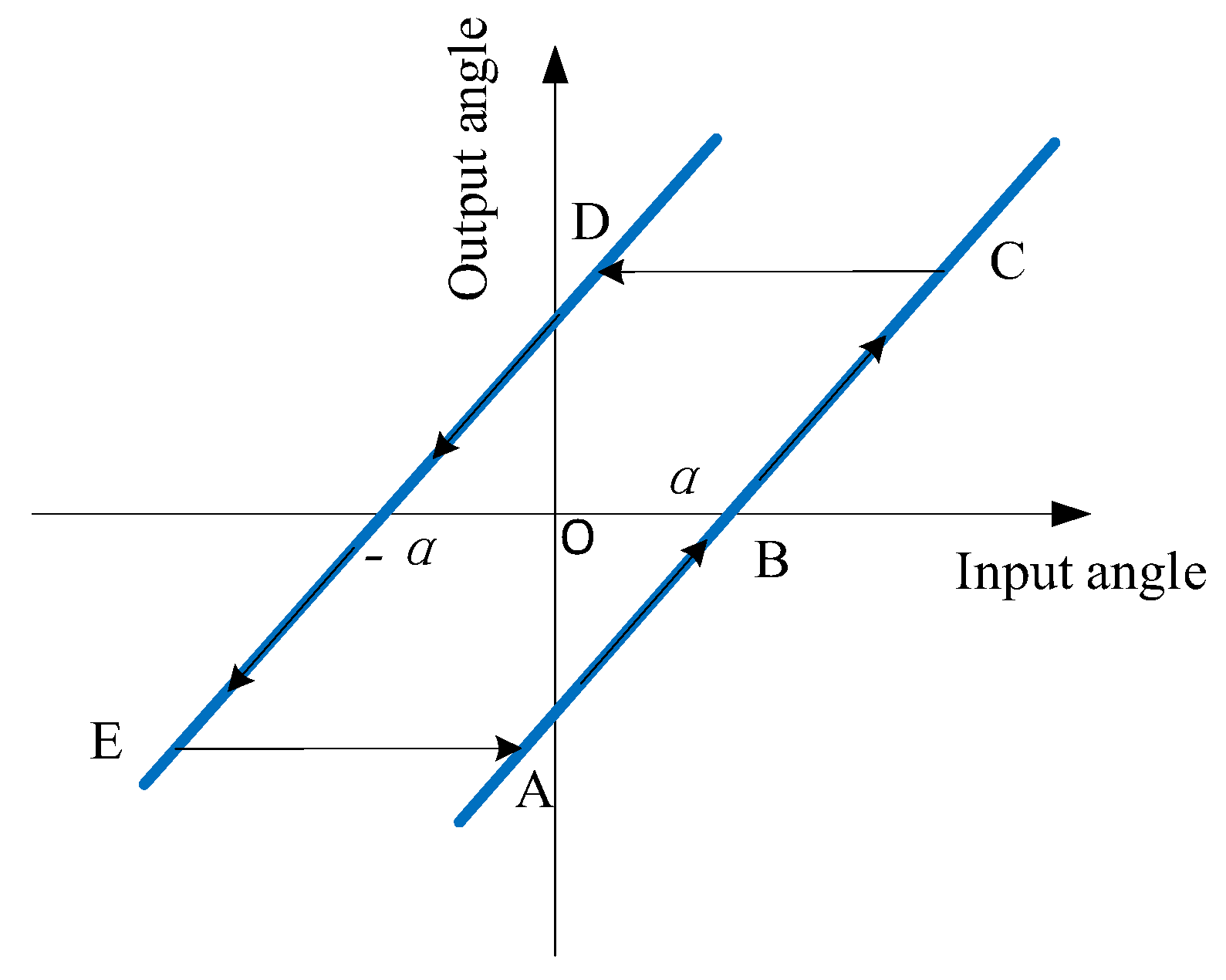
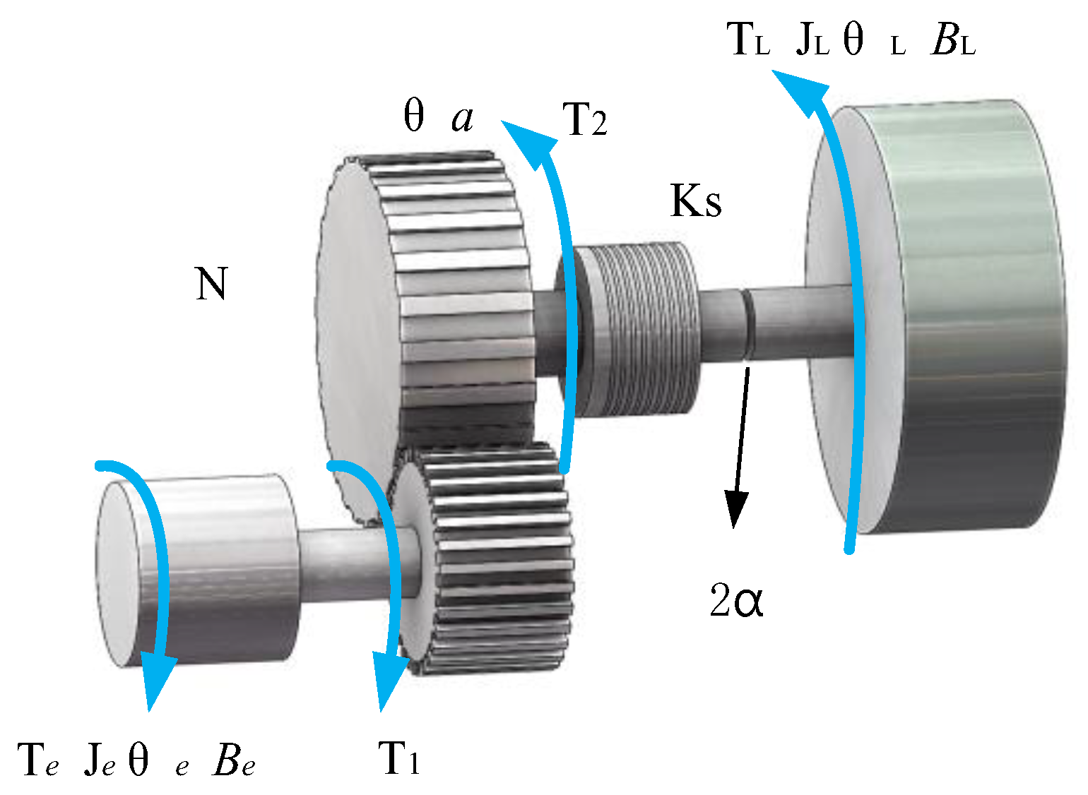
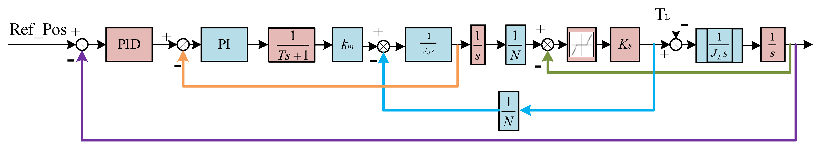
3.1. EMA Model with Gaps

Precision harmonic drives typically comprise flexible wheels, rigid wheels, and wave generators, as illustrated in Figure 4 [29]. In robot joints, the rigid wheel of the EMA remains stationary, while the rotor connects to the wave generator, and the flexible wheel acts as the driven component. The wave generator commonly consists of thin-walled flexible rolling ball bearings and standard elliptical cams. Upon installation of the wave generator into the flexible wheel, the latter deforms into an elliptical shape, facilitating partial contact between the outer ring gear of the flexible wheel and the inner ring gear of the rigid wheel. Typically, around 30% of the gears engage during operation. Acting as the active component in the harmonic drive, the wave generator induces a controllable elastic deformation of the flexible wheel when it rotates, facilitating motion and power transmission. The gear count difference between the flexible and rigid gears usually stands at two, with the transmission ratio defined as i = −Z2/(Z1 − Z2), where Z1 and Z2 represent the number of teeth on the rigid and flexible gears, respectively.

In the harmonic drive transmission system, a minor gap is maintained on the non-working surface during gear meshing to accommodate lubricating oil, reducing friction, and preventing jamming. This setup results in a large clearance with relatively low friction, while a small clearance leads to higher friction. Additionally, clearance compensates for dimensional deviations caused by temperature changes and elastic deformation, crucial for effective EMA transmission. Figure 5 illustrates the impact of the EMA gap factor on input and output. When the rotor’s rotation angle is below the gap threshold, the output end of the flexible wheel remains static, known as the OB section or the dead zone. As the rotation angle exceeds the gap, the flexible wheel starts rotating, and the input and output exhibit a deceleration ratio relationship, corresponding to the BC section. To reverse its motion with the rotor’s direction change, the rotation angle must surpass twice the OB, labeled as the CD segment. Once the rotation angle exceeds twice the OB value, the flexible wheel begins reverse movement, aligning with the DE segment. Similarly, changing the rotor’s direction requires traversing the EA section for the flexible wheel to alter its direction and proceed along the AC section.

In the harmonic drive transmission system, the pathway from the motor to the load can be simplified as a transmission with concentrated masses, separated by elastic elements and gaps. When we consider the motor and wave generator as one mass system, and the flexible wheel along with the load as another, the EMA system simplifies into a dual mass system [30,31]. According to Equation (2), the motor’s torque T_e is modulated by controlling the torque current i_q. Given the fast response of the current, the motor’s output torque is seen as an ideal torque source. Considering the impact of gap factors, Figure 6 illustrates the schematic representation of the EMA dual mass system model. Here, T_e, J_e, θ_e, and B_e symbolize the electromagnetic torque, moment of inertia, rotor angle, and damping coefficient at the motor end, respectively. Conversely, T_L, J_L, θ_L, and B_L denote the torque, moment of inertia, angle, and damping coefficient at the output end of the harmonic drive, respectively. N signifies the reduction ratio of the harmonic drive, Ks the stiffness coefficient, and 2α the gap in the transmission system. T₁ and T₂ represent the transmission torque driven by the model.

If there are no gaps in the system, then

$$\left\{\begin{array}{l}{T}_1=\frac{T_2}{N}\\ T_2=K_s\Delta \theta \\ \Delta \theta =(\frac{1}{N}{\theta }_e-{\theta }_L)\end{array}\right.$$

(7)

The relative angular displacement Δθ can be obtained from the transmission error calculation formula, with the transmission error expressed as

$$T_{e\_error}={\theta }_{out}-\frac{{\theta }_{in}}{N}$$

(8)

Given that the transmission error is defined as the angular displacement at the output end minus the angular displacement at the input end divided by the reduction ratio, to align the direction of T₁ consistent with the sign of the relative displacement, the opposite value of transmission errors is considered here. The influence of gap factors is disregarded based on the EMA dynamic model depicted in Figure 6.

$$\left\{\begin{array}{l}{J}_e{\ddot{\theta }}_e+B_e{\dot{\theta }}_e=T_e-T_1\\ \\ J_L{\ddot{\theta }}_L+B_L{\dot{\theta }}_L=T_2-T_L\end{array}\right.$$

(9)

Ignoring the damping effect in the system and combining Equations (7)–(9) can be transformed into

$$\left\{\begin{array}{l}{J}_e{\ddot{\theta }}_e+\frac{K_s}{N}\Delta \theta =T_e\\ \\ J_L{\ddot{\theta }}_L-K_s\Delta \theta =-T_L\end{array}\right.$$

(10)

When characterizing the nonlinear clearance model of the transmission system, commonly used models include the hysteresis model, dead zone model, and “vibration impact” model. The dead zone model takes the relative displacement as its input, with the output torque determined by multiplying this relative displacement by the stiffness coefficient. This model delineates the torque transmission relationship between the driving and driven components. In scenarios where a gap exists in the EMA, power transmission requires the relative displacement ΔθΔθ to exceed the gap. This nonlinear gap factor is represented using a dead zone function. The formulation of the dead zone model is provided in Equation (11), and its graphical representation is depicted in Figure 7.

$$\left\{\begin{array}{l}f(\Delta \theta ,\alpha )=\left\{\begin{array}{l}\Delta \theta -\alpha \hspace{1em}\hspace{1em}\Delta \theta >\alpha \\ 0\hspace{1em}\hspace{1em}\hspace{1em}\hspace{1em}-\alpha <\Delta \theta <\alpha \\ \Delta \theta +\alpha \hspace{1em}\hspace{1em}\hspace{1em}\Delta \theta <-\alpha \end{array}\right.\\ T=Ks\ast f(\Delta \theta ,\alpha )\end{array}\right.$$

(11)

The nonlinear gap dead zone model captures the relationship between relative displacement and torque transmission, providing the advantage of simplicity in its expression. In the EMA transmission system, the nonlinear clearance is directly linked to the relative displacement Δθ between the input and output, making the dead zone model particularly suitable for practical scenarios involving EMA clearance.

The dynamic equation of the harmonic drive incorporating the gap factor added is represented by Equation (12), where the relationship between the driven output torque T₂ and the relative displacement Δθ of the gap model is T₂ = K_s∗f(Δθ, α). According to Equation (12), the dynamic equation of the harmonic drive with the gap factor added is

$$\left\{\begin{array}{l}{J}_e{\ddot{\theta }}_e+\frac{K_s}{N}\Delta \theta =T_e\\ J_L{\ddot{\theta }}_L-K_{s}f(\Delta \theta ,\alpha )=-T_L\end{array}\right.$$

(12)

Combining the EMA dynamic Equation (12) and adding a gap model, the control block diagram of the EMA containing nonlinear gaps is shown in Figure 8. PI is the speed loop controller, PID is the position loop controller, and k_m is the motor torque coefficient.

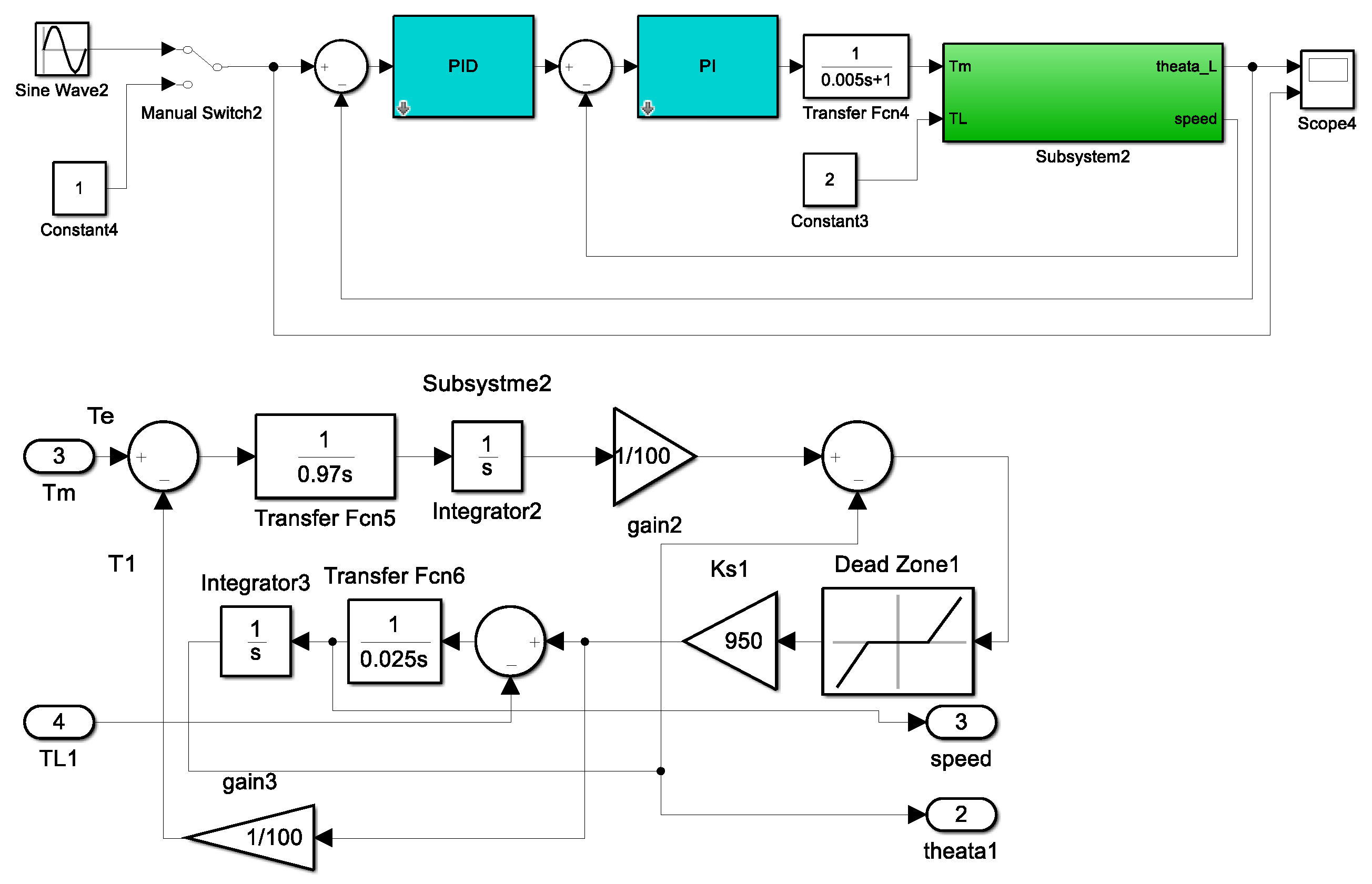
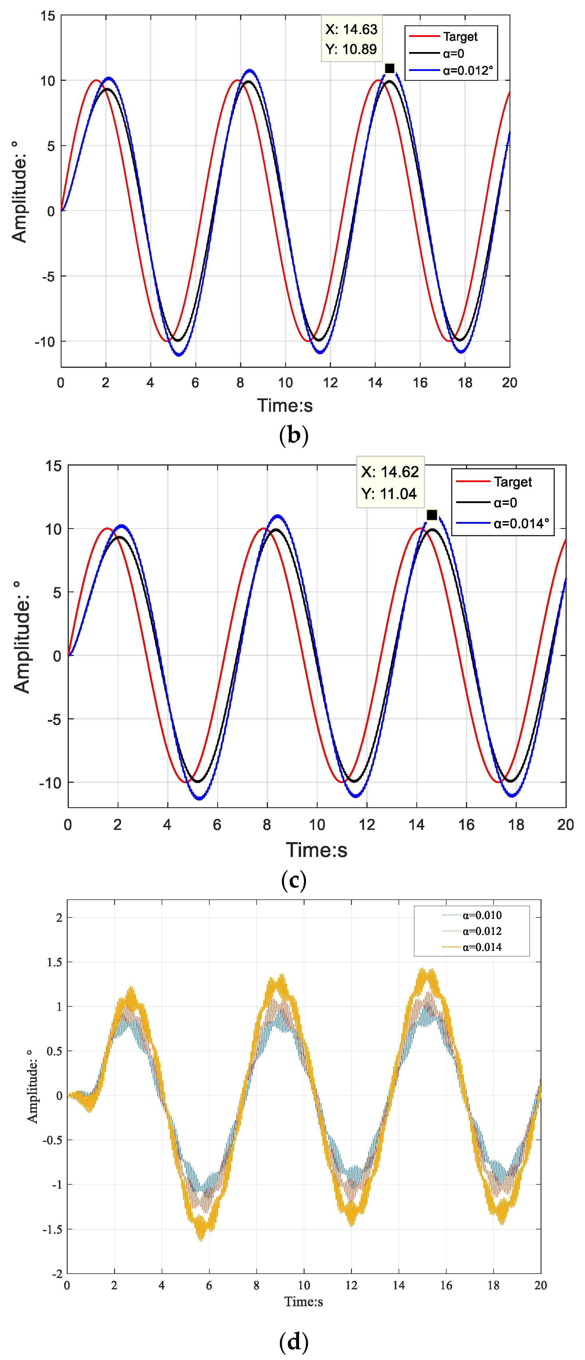
3.2. EMA Simulation Analysis with Gaps

As shown in Figure 7, α represents the clearance. Assigning α values of 0.010°, 0.012°, and 0.014° for simulation analysis, a simulation model is constructed based on the control block depicted in Figure 8. The model evaluates and compares the sinusoidal tracking characteristics of an EMA with and without clearance. Figure 9 illustrates a simulation model incorporating gaps, developed within the Simulink environment, and subjected to a load of T_L = 2 N·m. The simulation outcomes are presented in Figure 10.

The outcomes of the simulation, as shown in Figure 10, illustrate that as the gap increases, there is a gradual decrease in the EMA’s tracking performance, accompanied by a progressive increase in tracking error. Figure 10 presents the position tracking error values for different gap sizes, indicating that a larger gap results in higher tracking error and reduced tracking accuracy. This underscores the significant effect of clearance on the motion performance of the EMA, with an expectation that clearance will increase as the service duration of the EMA extends, thereby reducing the system’s tracking accuracy. Therefore, it is essential to compensate for the gap to improve the control accuracy of the system. Additionally, the simulation results emphasize that changes in the direction of motion worsen the position tracking error and degrade tracking performance as the gap widens. Consequently, the impact of clearance on EMA motion performance is considerable, necessitating compensation control for clearance to ensure optimal functioning.

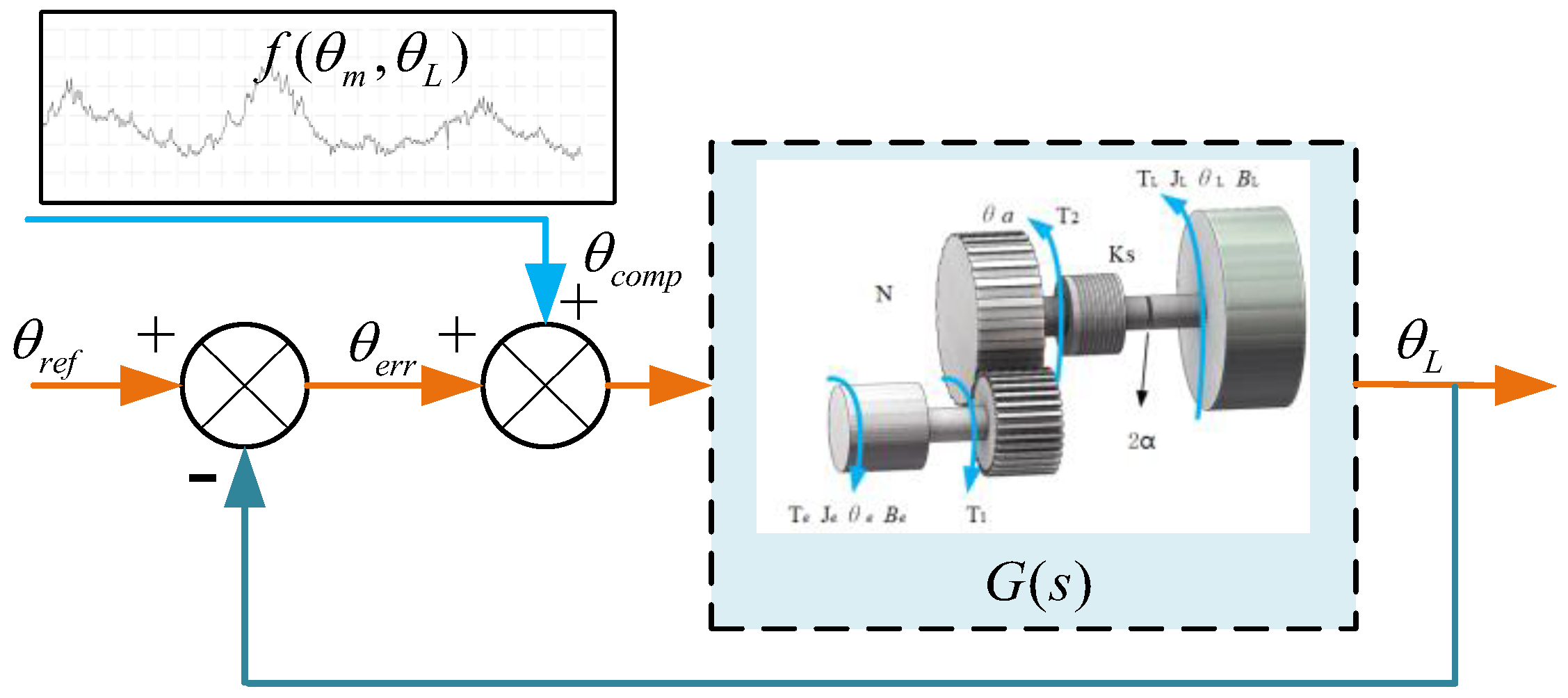
3.3. EMA Position Error Compensation

Position error refers to the difference between the actual output position and the theoretical output position. Compensating for position error is an effective strategy to reduce transmission error in EMA and improve control precision. The extent of transmission error is greatly affected by both speed and load, making online compensation necessary to enhance EMA’s control accuracy across various operational conditions. During the motion process, the position error signal is continuously computed in real time using input and output position sensors, enabling online position compensation to enhance the system’s tracking accuracy. Figure 11 illustrates the schematic representation of online compensation for position error.

In Figure 11, θ_ref denotes the prescribed position instruction sent by the external system, while θ_L represents the output angle of the micro transmission system. θ_err signifies the positional disparity between the designated value and the actual output value, whereas θ_comp indicates the position error compensation position. G(s) represents the controlled object, and N denotes the transmission ratio. In conventional control approaches, only θ_err is introduced as an error value into the closed-loop control system, neglecting the influence of positional error factors. This omission results in inferior control performance and tracking accuracy. Real-time calculation of position errors for the micro transmission systems is facilitated by θ_comp, the controller output. Utilizing θ_comp and other significant reverse position commands for position error compensation enhances the tracking accuracy of the EMA across different speeds and loads.

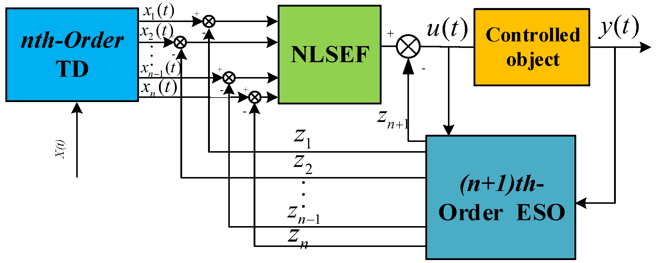
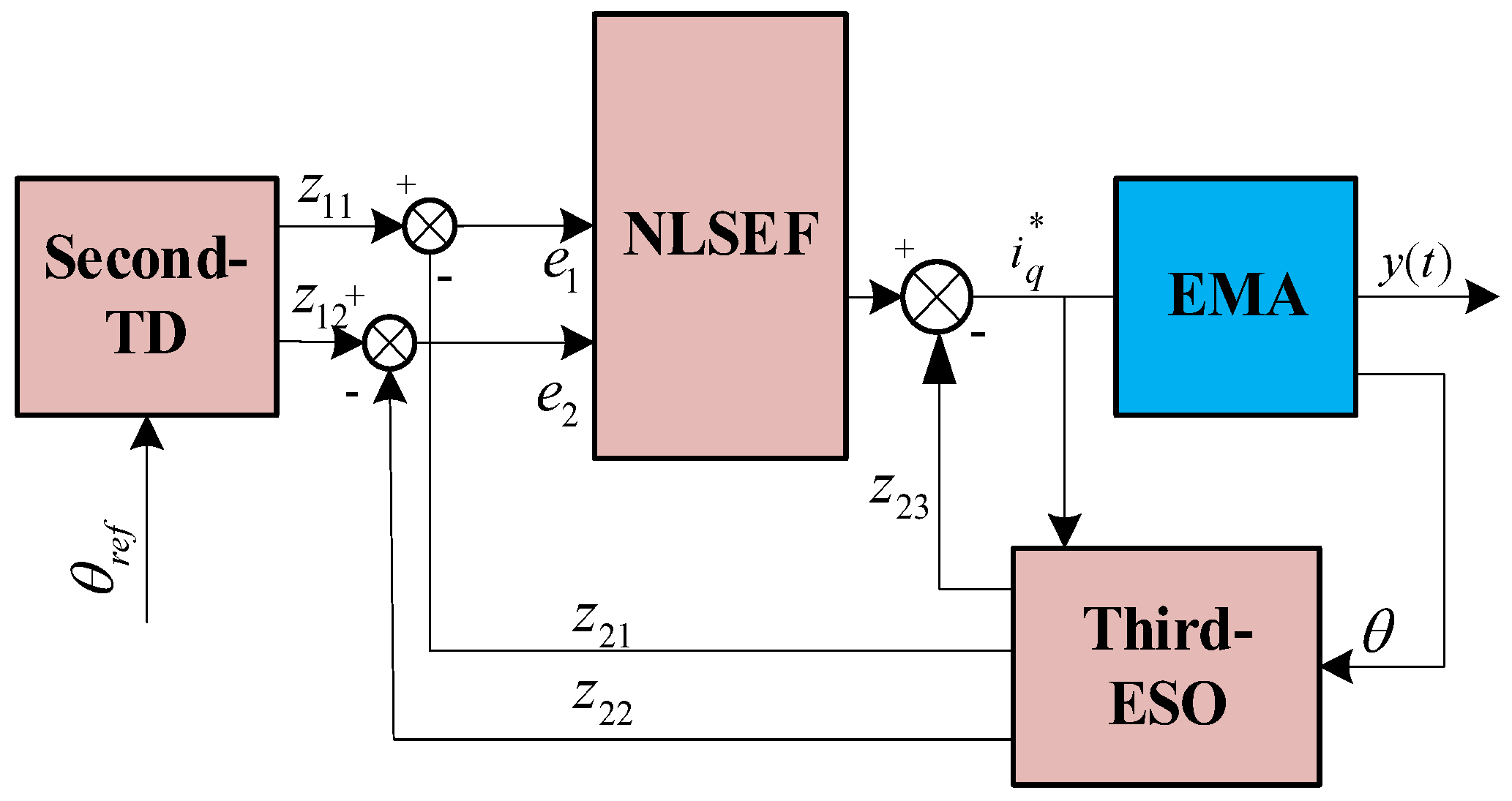
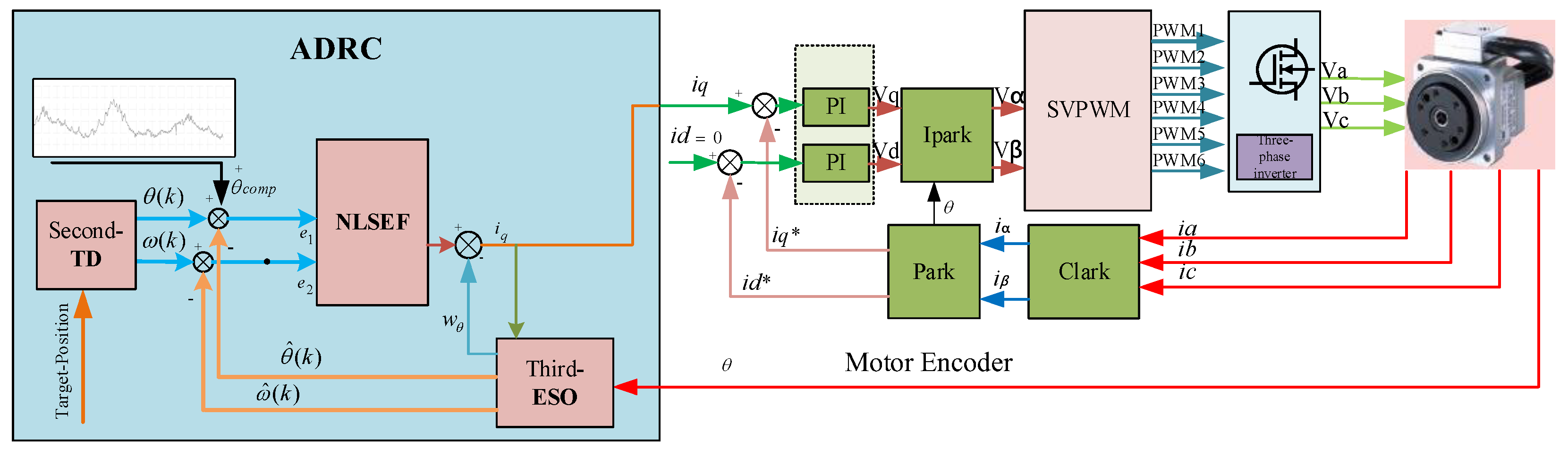
4. Position Loop Second-Order ADRC Design for Positional Errors

ADRC comprises a tracking differentiator (TD), an extended state observer (ESO), and nonlinear state error feedback (NLSEF) [32,33,34]. The tracking differentiator (TD) facilitates the tracking process by resolving the trade-off between overshoot and response speed, ensuring rapid and overshoot-free tracking of input signals. The extended state observer (ESO) monitors the system’s output, internal unmodeled factors, and external disturbances in real time. It compensates for these factors within the control law, significantly improving the system’s resistance to interference. NLSEF integrates nonlinearity by combining the output from TD with the state variable observation estimates from ESO. Simultaneously, the output from NLSEF merges with the “total disturbance” estimation from ESO to influence the controlled object. Figure 12 illustrates the schematic of ADRC.

In real-world situations, first- or second-order ADRC systems are often favored for their simplicity and effectiveness, whereas third-order and higher systems, with their more intricate formulations, see limited use. For designing the position loop, a proposal is made for employing a second-order ADRC. Drawing from the mechanical equation outlined in (13), it is possible to derive the dynamic mathematical model of the PMSM position loop, providing a robust framework for implementing precise control strategies and enhancing system performance by actively rejecting disturbances.

$$\frac{d^2\theta }{d{t}^2}=-\frac{B}{J}\omega -\frac{TL}{J}+\frac{3p_n{\Psi }_f}{2J}{i}_q$$

(13)

where θ is the rotor position and ω is the differential of θ. The control quantity is set to u = i_q, the known disturbance is $f(x_1,x_2)=-\frac{B\omega }{J}$, the unknown disturbance is $w(t)=-\frac{T_L}{J}$, and $b=1.5\frac{p_n{\Psi }_f}{J}$. θ can be measured through a position sensor. Setting x_{1 =} θ, x_{2 =} ω, $f_1(x_1,x_2)=-\frac{B}{J}\omega$, $f_2(x_1,x_2,t)=-\frac{T_L}{J}$, $b=\frac{3p_n{\Psi }_f}{2J}$, and $u=i_q$, the second-order state equation for constructing a position loop is

$$\left\{\begin{array}{l}{x}_1=x_2=\frac{d\theta }{dt}\\ {\dot{x}}_2=\frac{d^2\theta }{d{t}^2}=f_1(x_1,x_2)+f_2(x_1,x_2,t)+bu\\ y=x_1=\theta \end{array}\right.$$

(14)

Based on Equation (14), a second-order active disturbance rejection expression for the position loop can be formulated. The block diagram illustrating the second-order ADRC control of the position loop is depicted in Figure 13. where θ_ref is the given target position and is the torque current output by the ADRC. z₁₁ and z₂₁ are the tracking signals of θ_ref and θ, z₁₂ and z₂₂ are the differential signals of z₁₁ and z₂₁, and z₂₃ is the tracking signal of interference signal w(t).

The expression for the TD term in the second-order ADRC of the position loop is depicted in Equation (15):

$$\left\{\begin{array}{l}fhan\_pos(\cdot )=fhan(\theta (k)-{\theta }_{ref},\omega (k),r,h)\\ \theta (k+1)=\theta (k)+T\omega (k)\\ \omega (k+1)=\omega (k)+Tfhan\_pos(\cdot )\end{array}\right.$$

(15)

where θ_ref represents the target position and θ(k) and ω(k) represent the angle and velocity, respectively, during the process of reaching the target position. At steady state, θ = θ_ref. During the operation of the EMA toward the target position, the ESO can estimate the disturbance z₃ during the motion process in real time and compensate for it. r is the speed factor that determines the tracking speed, T is the integration step size, and h is the filtering factor. The larger h is, the more obvious the filtering effect.

The ESO representation of the second-order ADRC of the position loop is

$$\left\{\begin{array}{l}e=\widehat{\theta }(k)-\theta (k)\\ \widehat{\theta }(k+1)=\widehat{\theta }(k)+T(\widehat{\omega }(k)-{\beta }_{01}e)\\ \widehat{\omega }(k+1)=\widehat{\omega }(k)+T(w_{\theta }(k)-{\beta }_{02}fal(e,{\alpha }_{01},\delta )+b_0{i}_q(k))\\ w_{\theta }(k+1)=w_{\theta }(k)-T{\beta }_{03}fal(e,{\alpha }_{02},\delta )\end{array}\right.$$

(16)

where $\widehat{\theta }(k)$ and $\widehat{\omega }(k)$ are the estimated values of θ(k) and ω(k), respectively. w_θ(k) is the disturbance observed during the motion of the position loop. δ is an adjustable parameter, and δ is recommended to take the same value as h. Generally, the values of α₀₁ and α₀₂ are 0.5 and 0.25, respectively. The expression for constructing the position loop NLSEF based on the TD output and ESO output is shown in Equation (17):

$$\left\{\begin{array}{l}{e}_1(k)=\theta (k)-\widehat{\theta }(k)\\ e_2(k)=\omega (k)-\widehat{\omega }(k)\\ {\widehat{i}}_q(k)={\beta }_{1}fal(e_1(k),{\alpha }_1,\delta )+{\beta }_{2}fal(e_2(k),{\alpha }_2,\delta )\\ i_q(k)={\widehat{i}}_q(k)-\frac{w_{\theta }(k)}{b_0}\end{array}\right.$$

(17)

In Equation (17), the formulations for the optimal comprehensive control functions fhan(∙) and fal(∙) are as follows:

$$\begin{array}{l}fhan=\left\{\begin{array}{l}d=rh;\hspace{1em}\hspace{1em}\hspace{1em}{d}_0=hd\\ y=x_1+h_1{x}_2-v(k);\hspace{1em}\hspace{1em}\hspace{1em}{a}_0=\sqrt{d^2+8r\left|y\right|}\\ a=\left\{\begin{array}{l}{x}_2+\frac{(a_0-d)}{2},\left|y\right|>d_0\\ x_2+\frac{y}{h_1},\left|y\right|\le d_0\end{array}\right.\\ fst=\left\{\begin{array}{l}-\frac{ra}{d},\left|a\right|\le d\\ -rsign(a),\left|a\right|>d\end{array}\right.\end{array}\right.\\ fal=\left\{\begin{array}{l}{\left|e\right|}^{\alpha }sign(e),\left|e\right|>\delta \\ \frac{x}{{\delta }^{(1-\alpha )}},\left|e\right|\le \delta \end{array}\right.\end{array}$$

(18)

where α is a nonlinear factor and e is an error variable. The fal(∙) function has the characteristic of “small error with a large gain, large error with small gain”.

In the EMA control system, an FOC control strategy is employed. Unlike the three closed-loop cascade PI control modes, the second-order ADRC combines the position loop and speed loop into a speed/position composite controller. Here, the transmission error signal is introduced into the θ(k) link of the ADRC, thereby enhancing the system’s tracking accuracy under different speeds and loads through online position compensation. The ADRC control block diagram for position error is shown in Figure 14.

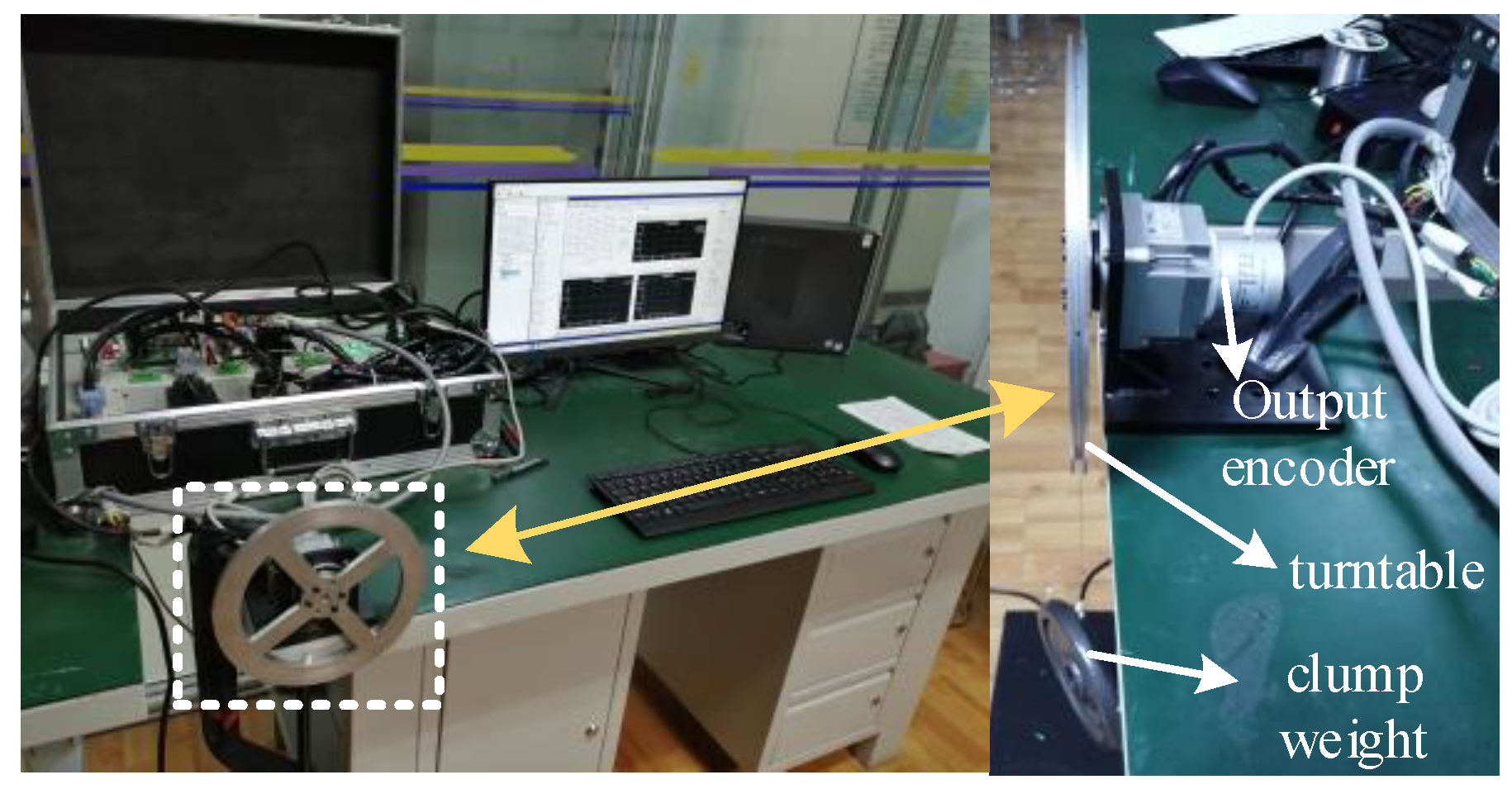
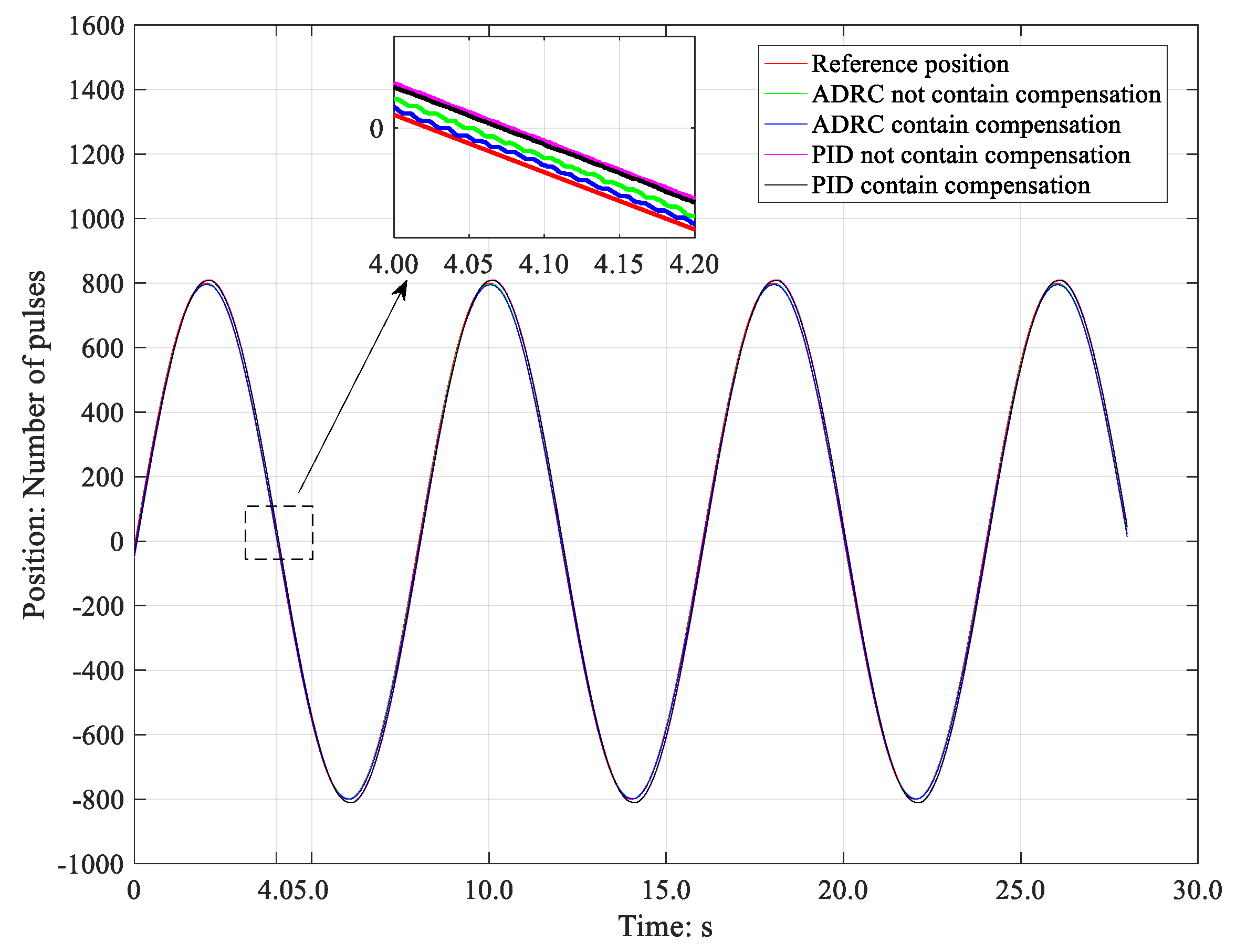
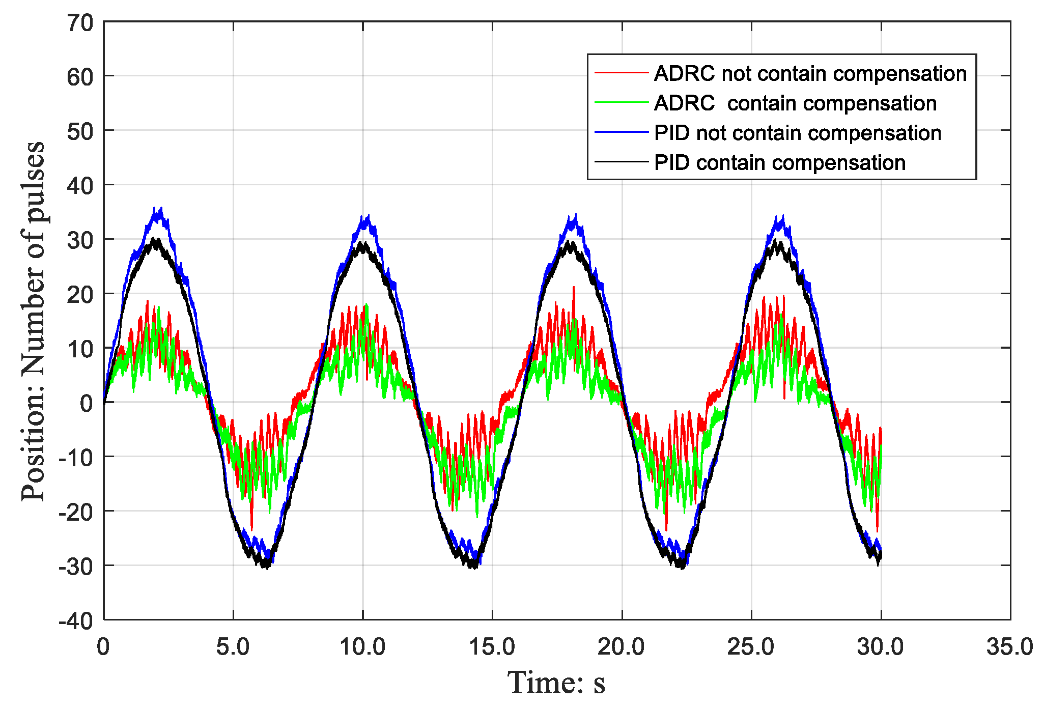
5. Experimental Analysis

To evaluate the effectiveness of ADRC in compensating for position error, experimental validation and analysis were conducted using the RT Cube platform. This platform enables seamless transition from simulation models to physical control implementations. The experiments involved comparing the tracking accuracy of PID and ADRC control strategies, with and without position error compensation, under different speeds and loads.

The experimental setup is depicted in Figure 15. High-precision encoders are installed both at the rotor end of the EMA motor and at the output end of the harmonic reducer to ensure precise measurement of angular positions. For loading purposes, a hanging counterweight system is utilized, providing stability and precision advantages over alternative methods such as torque motors and magnetic powder brakes. Throughout the tests, the electric machine operates at a rated voltage of 24 V, the harmonic reducer has a reduction ratio of 50, and the counterweight block weighs 2.5 kg. Additionally, the turntable has a radius of 0.1 m, the encoder at the motor rotor end has a resolution of 2000 PPR, and the output encoder of the harmonic reducer offers 20,000 PPR, ensuring detailed and accurate feedback for control analysis.

The input and output encoders of the EMA can achieve 8000 PPR and 80,000 PPR, respectively, after quadrupling the frequency. With the given target sine signal Pref = 4000 × sin (2π × 0.25t), and considering the reduction ratio of the harmonic reducer alongside the resolution of the output encoder, the theoretical positional change of the output end is Pout = 800 × sin (2π × 0.25t). The position output curves of several different control methods are shown in Figure 16.

The evaluation of position control accuracy for the PID and ADRC control modes is conducted using peak-to-peak error, root mean square error (RMSE), and mean absolute error (MAE) as assessment indicators. The RMSE expression is given by

$$e\_rmse=\sqrt{[{\displaystyle \sum _{i=1}^n{e}^2(i)}]/n}$$

(19)

The expression for the MAE is

$$e\_mae=\frac{1}{n}{\displaystyle \sum _{i=1}^n\left|e(i)\right|}$$

(20)

Table 1. Comparison of no-load compensation experimental results.

Control Mode	Peak to Peak	RMSE	MAE
PID	65.671	21.558	19.425
PID-compensation	60.965	20.592	18.533
ADRC	45.000	9.121	7.898
ADRC-compensation	39.283	8.799	7.389

shows the calculation results of the peak-to-peak, RMSE, and MAE for the four control modes in the no-load mode.

Figure 17 and

Table 2. Comparison of the load compensation experiment results.

Control Mode	Peak to Peak	RMSE	MAE
PID	76.917	26.376	23.698
PID-compensation	68.419	23.468	21.139
ADRC	40.488	9.566	8.343
ADRC-compensation	33.867	9.046	7.631

illustrate that the addition of friction feedforward compensation leads to improvements in the peak-to-peak value, root mean square error, and average absolute error of the position error.

During the load experiment, a 2.5 kg counterweight is attached to the turntable with a radius of 0.1 m, resulting in a 2.5 N∙m load applied to the EMA. The sinusoidal target signal provided is identical to the signal used in the no-load scenario. Figure 18 displays the error variation curve between the actual output position and the theoretical output position under different load control methods.

Table 2 displays the calculation results of the peak-to-peak, root mean square error, and average absolute error for the four control modes under the load condition.

Figure 18 and Table 2 illustrate that with the addition of position error compensation, there are improvements in the peak-to-peak, root mean square error, and average absolute error of the position error. The PID with position error compensation reduces the peak-to-peak value by around 8.5, the root mean square error by approximately 3.1, and the average absolute error by about 2.5 compared to the PID alone. Similarly, compared to the ADRC, the ADRC with position error compensation decreases the peak-to-peak value by approximately 6.612, the root mean square error by about 0.52, and the average absolute error by roughly 0.712.

6. Conclusions

The article investigates how variations in gap affect the accuracy of position tracking in EMA systems equipped with harmonic deceleration. It explores the efficacy of position error compensation and ADRC methods in addressing this issue. Beginning with the development of a mathematical model for the PMSM, the study derives transfer functions for current and speed loop controls. A simulation model for an EMA with varying gaps is then created, followed by analysis to understand how different gap sizes impact the position tracking accuracy. Following this, an online compensation model for EMA position error is developed by computing the position error signal in real time. The principles of a second-order active disturbance rejection controller are examined, leading to the design of a controller for EMA position mode that integrates the online position error model. Experimental evaluations on the RT Cube platform compare four control approaches—PID, position error compensation PID, ADRC, and position error compensation ADRC—in sinusoidal position tracking experiments. Peak-to-peak, root mean square error, and absolute error are used as evaluation metrics. The experimental results, conducted under both no-load and load conditions, reveal that ADRC performs better than PID in terms of tracking accuracy. Additionally, incorporating position error compensation further improves control precision. Notably, the root mean square error of the position error compensation–ADRC under loaded conditions is significantly lower than that of the PID control method. The integration of ADRC and the inclusion of position error compensation are identified as crucial factors in enhancing the positional accuracy of EMA systems. By compensating for position errors online, the position accuracy of EMA can be improved under different working conditions.

References

1. Jung, B.J.; Kim, B.; Koo, J.C.; Choi, H.R.; Moon, H. Joint torque sensor embedded in harmonic drive using order tracking method for robotic application. IEEE/ASME Trans. Mechatron. 2017, 22, 1594–1599. [Google Scholar] [CrossRef]
2. Ismail, M.A.A.; Windelberg, J.; Liu, G. Simplified sensorless torque estimation method for harmonic drive based electro-mechanical actuator. IEEE Robot. Autom. Lett. 2021, 6, 835–840. [Google Scholar] [CrossRef]
3. Chen, Y.Y.; Huang, P.Y.; Yen, J.Y. Frequency-domain identification algorithms for servo systems with friction. IEEE Trans. Control Syst. Technol. 2002, 10, 654–665. [Google Scholar] [CrossRef]
4. Han, B.C.; Ma, J.J.; Li, H.T. Modeling and compensation of nonlinear friction in harmonic driver. Opt. Precis. Eng. 2011, 19, 1095–1103. [Google Scholar]
5. Han, B.C.; Ma, J.J.; Li, H.T. Research on nonlinear friction compensation of harmonic drive in gimbal servo-system of DGCMG. Int. J. Control Autom. Syst. 2016, 14, 779–786. [Google Scholar] [CrossRef]
6. Shi, Y.; Yu, Y.; Wang, Q.; Li, H.; Chen, X. Composite Control Based on Feed-Forward and FISMC Method for Accurate Speed of Gimbal System wth Harmonic Drive. IEEE Trans. Power Electron. 2023, 38, 6434–6443. [Google Scholar] [CrossRef]
7. Ostapski, W. Analysis of the stress state in the harmonic drive generator-flexspline system in relation to selected structural parameters and manufacturing deviations. Bull. Pol. Acad. Sci.-Tech. Sciences. Sci. 2010, 58, 683–698. [Google Scholar] [CrossRef]
8. Han, J. Active disturbance rejection controller and its applications. Control Decis. 1998, 13, 19–23. (In Chinese) [Google Scholar]
9. Han, J. From PID to active disturbance rejection control. IEEE Trans. Ind. Electron. 2009, 56, 900–906. [Google Scholar] [CrossRef]
10. Gao, Z. Scaling and Parameterization Based Controller Tuning. In Proceedings of the 2003 American Control Conference, Denver, CO, USA, 4–6 June 2003. [Google Scholar]
11. Guo, B.Z.; Jin, F.F. The active disturbance rejection and sliding mode control approach to the stabilization of the Euler–Bernoulli beam equation with boundary input disturbance. Automatica 2013, 49, 2911–2918. [Google Scholar] [CrossRef]
12. Tian, M.; Wang, B.; Yu, Y.; Dong, Q.; Xu, D. Discrete-time repetitive control-based ADRC for current loop disturbances suppression of PMSM drives. IEEE Trans. Ind. Inform. 2021, 18, 3138–3149. [Google Scholar] [CrossRef]
13. Hezzi, A.; Ben Elghali, S.; Bensalem, Y.; Zhou, Z.; Benbouzid, M.; Abdelkrim, M.N. ADRC-based robust and resilient control of a 5-phase PMSM driven electric vehicle. Machines 2020, 8, 17. [Google Scholar] [CrossRef]
14. Su, Y.X.; Zheng, C.H.; Duan, B.Y. Automatic disturbances rejection controller for precise motion control of permanent-magnet synchronous motors. IEEE Trans. Ind. Electron. 2005, 52, 814–823. [Google Scholar] [CrossRef]
15. Li, S.; Xia, C.; Zhou, X. Disturbance rejection control method for permanent magnet synchronous motor speed regulation system. Mechatronics 2016, 22, 706–714. [Google Scholar] [CrossRef]
16. Rong, Z.; Huang, Q. A new PMSM speed modulation system with sliding mode based on active-disturbance-rejection control. J. Cent. South Univ. 2016, 23, 1406–1415. [Google Scholar] [CrossRef]
17. Li, S.; Liu, Z. Adaptive speed control for permanent-magnet synchronous motor system with variations of load inertia. IEEE Trans. Ind. Electron. 2009, 56, 3050–3059. [Google Scholar]
18. Zhu, H.; Weng, F.; Li, D.; Zhu, M. Active control of combustion oscillation with active disturbance rejection control (ADRC) method. J. Sound Vib. 2022, 540, 117245. [Google Scholar] [CrossRef]
19. Liu, Y.; Wen, J.; Xu, D.; Huang, Z.; Zhou, H. The decoupled vector-control of PMSM based on nonlinear multi-input multi-output decoupling ADRC. Adv. Mech. Eng. 2020, 12, 1687814020984255. [Google Scholar] [CrossRef]
20. Kang, K.; Song, J.; Kang, C.; Sung, S.; Jang, G. Real-time detection of the dynamic eccentricity in permanent-magnet synchronous motors by monitoring speed and back EMF induced in an additional winding. IEEE Trans. Ind. Electron. 2017, 64, 7191–7200. [Google Scholar] [CrossRef]
21. Huang, Y.; Huang, W.; Chen, S.; Liu, Z. Complementary sliding mode control with adaptive switching gain for PMSM. Trans. Inst. Meas. Control 2019, 41, 3199–3205. [Google Scholar] [CrossRef]
22. Lee, K.; Hong, S.; Oh, J.-H. Development of a Lightweight and High-efficiency Compact Cycloidal Reducer for Legged Robots. Int. J. Precis. Eng. Manuf. 2019, 21, 415–425. [Google Scholar] [CrossRef]
23. Qi, L.; Bao, S.; Shi, H. Permanent-magnet synchronous motor velocity control based on second-order integral sliding mode control algorithm. Trans. Inst. Meas. Control 2013, 37, 875–882. [Google Scholar] [CrossRef]
24. Jin, R.; Wang, J.; Ou, Y.; Li, J. Composite ADRC Speed Control Method Based on LTDRO Feedforward Compensation. Sensors 2024, 24, 2605. [Google Scholar] [CrossRef]
25. Gao, S.; Wei, Y.; Zhang, D.; Qi, H.; Wei, Y. A Modified Model Predictive Torque Control with Parameters Robustness Improvement for PMSM of Electric Vehicles. Actuators 2021, 10, 132. [Google Scholar] [CrossRef]
26. Yi, Y.; Sun, X.; Li, X.; Fan, X. Disturbance observer based composite speed controller design for PMSM system with mismatched disturbances. Trans. Inst. Meas. Control 2015, 38, 742–750. [Google Scholar] [CrossRef]
27. Moon, H.T.; Kim, H.S.; Youn, M.J. A discrete-time predictive current control for PMSM. IEEE Trans. Power Electron. 2003, 18, 464–472. [Google Scholar] [CrossRef]
28. Zhang, X.; Zhang, L.; Zhang, Y. Model predictive current control for PMSM drives with parameter robustness improvement. IEEE Trans. Power Electron. 2018, 34, 1645–1657. [Google Scholar] [CrossRef]
29. Ghorbel, F.H.; Gandhi, P.S.; Alpeter, F. On the kinematic error in harmonic drive gears. J. Mech. Des. 2001, 123, 90–97. [Google Scholar] [CrossRef]
30. Roozing, W.; Malzahn, J.; Kashiri, N.; Caldwell, D.G.; Tsagarakis, N.G. On the stiffness selection for torque-controlled series-elastic actuators. IEEE Robot. Autom. Lett. 2017, 2, 2255–2262. [Google Scholar] [CrossRef]
31. Ishida, T.; Takanishi, A. A robot actuator development with high back drivability. In Proceedings of the 2006 IEEE Conference on Robotics, Automation and Mechatronics, Bangkok, Thailand, 1–3 June 2006; pp. 1–6. [Google Scholar]
32. Han, J.; Wang, H.; Jiao, G.; Cui, L.; Wang, Y. Research on active disturbance rejection control technology of electromechanical actuators. Electronics 2018, 7, 174. [Google Scholar] [CrossRef]
33. Huang, Z.; Liu, Y.; Zheng, H.; Wang, S.; Ma, J.; Liu, Y. A self-searching optimal ADRC for the pitch angle control of an underwater thermal glider in the vertical plane motion. Ocean Eng. 2018, 159, 98–111. [Google Scholar] [CrossRef]
34. Gao, C.; Yuan, J.; Zhao, Y. ADRC for spacecraft attitude and position synchronization in libration point orbits. Acta Astronaut. 2018, 145, 238–249. [Google Scholar] [CrossRef]
Figure 1. Current loop control block diagram.
Energies 17 02528 g001
Figure 2. Speed loop control block diagram.
Energies 17 02528 g002
Figure 3. Simplified block diagram of speed loop control.
Energies 17 02528 g003
Figure 4. Structural diagram of the harmonic reducer.
Energies 17 02528 g004
Figure 5. The influence of nonlinear gap factors on the input and output.
Energies 17 02528 g005
Figure 6. EMA two-quality system model diagram.
Energies 17 02528 g006
Figure 7. Dead zone model diagram.
Energies 17 02528 g007
Figure 8. Block diagram of the EMA control system with gaps.
Energies 17 02528 g008
Figure 9. EMA gap simulation model.
Energies 17 02528 g009
Figure 10. (a) EMA position output under sinusoidal target input. Clearance α = 0.010°; (b) EMA position output under sinusoidal target input. Clearance α = 0.012°; (c) EMA position output under sinusoidal target input. Clearance α = 0.014°; (d) error data of different clearances.
Energies 17 02528 g010aEnergies 17 02528 g010b
Figure 11. Online position error compensation block diagram.
Energies 17 02528 g011
Figure 12. ADRC control block diagram.
Energies 17 02528 g012
Figure 13. Position loop second-order ADRC.
Energies 17 02528 g013
Figure 14. ADRC control block diagram for position error compensation.
Energies 17 02528 g014
Figure 15. Experimental platform for the position error compensation of the EMA.
Energies 17 02528 g015
Figure 16. Output position change curve.
Energies 17 02528 g016
Figure 17. The change in the no-load position error.
Energies 17 02528 g017
Figure 18. Changes in the load position error.
Energies 17 02528 g018