Modeling and Prediction of Carbon Monoxide during the Start-Up in ICE through VARX Regression

Abstract

In a global society that is increasingly interrelated and focused on mobility, carbon monoxide emissions derived from internal combustion vehicles remain the most important factor that must be addressed to improve environmental quality. Certainly, air pollution generated by internal combustion engines threatens human health and the well-being of the planet. In this regard, this paper aims to address the urgent need to understand and face the CO emissions produced by internal combustion vehicles; therefore, this work proposes a mathematical model based on Auto-Regressive Exogenous that predicts the CO percentages produced by an internal combustion engine during its start-up. The main goal is to establish a strategy for diagnosing excessive CO emissions caused by changes in the engine temperature. The proposed CO emissions modeling is evaluated under a real dataset obtained from experiments, and the obtained results make the proposed method suitable for being implemented as a novel diagnosis tool in automotive maintenance programs.

1. Introduction

Nowadays, environmental pollution is a global problem that affects the health of the world’s population, in this regard, to face this issue it is important to understand the reasons and sources that lead to the generation of high levels of environmental pollution. Certainly, there exist three main types of pollution that must be primarily considered: air, water, and soil, where air pollution involves the presence of harmful chemical particles in the air at high concentrations that can be detrimental to plant, animal, and human life. Accordingly, the presence of compounds that degrade the air quality has contributed to climate change and ozone depletion, which negatively impact life on Earth. On the other hand, fossil fuels release harmful atmospheric pollutants even before being burned. Indeed, the need to fulfill all energy requirements demanded by humans has been performed through the combustion of oil, coal, and gas; however, these practices are some of the main sources that contribute to the current global warming crisis. The burning of these fossil fuels produces a range of pollutants, both primary and secondary, such as suspended particles, sulfur dioxide ($\mathrm{S}{\mathrm{O}}_2$), carbon dioxide ($\mathrm{C}{\mathrm{O}}_2$), carbon monoxide (CO), hydrocarbons, organic compounds, chemicals, and nitrogen oxides (NOx). These emissions contain the major greenhouse gases, such as $\mathrm{C}{\mathrm{O}}_2$, methane (CH4), NOx, and fluorinated gases. Therefore, air pollution derived from these activities not only poses a threat to air quality but also partially contributes to climate change and global warming [1]. Specifically, CO is formed when the combustion of fossil fuel is incomplete, so the main sources of CO in the world are energy producers and consumers, such as industry, commerce, and transportation, primarily using coal, oil, and natural gas. The Scenario of Declared Policies (STEPS) forecasts a CO decrease of about 73% by 2030; however, this decrease would be insufficient to achieve global climate goals if the consumption of these fossil fuels remains high [2]. In an increasingly interconnected world that is dependent on mobility, the reduction in CO emissions produced by internal combustion engine vehicles (ICEVs) represents an environmental challenge [3]. Although ICEVs are vital for progress and convenience, they are also an insidious source of pollution that endangers the quality of life and the well-being of the planet [4]. In recent years, emissions resulting from ICEVs, such as CO, NOx, $\mathrm{C}{\mathrm{O}}_2$, and $\mathrm{S}{\mathrm{O}}_2$, have increased due to the high demand of mobility, especially $\mathrm{C}{\mathrm{O}}_2$ in 2022 [5]. It is also important to mention that in the case of compression ignition engines, the temperature inside significantly influences the emission of toxic gases, i.e., diesel engines are exposed to undergo important thermal processes during the combustion process. Accordingly, the determination of the heat dissipation during operation allows us to check the combustion of the air–fuel mixture in the engine. Hence, burning 50% of the fuel dose allows a relative determination of the combustion phase, which means an angular position at 50% of the heat production. This indicator could be used to control combustion in the diesel engine, reducing the emission of toxic components. For example, by dividing the fuel injection into two parts, the first at 10° before top dead center of compression (BTDC) and the second at 50° BTDC, unburned methane (${\mathrm{CH}}_4$) emissions and $\mathrm{C}{\mathrm{O}}_2$ emissions are reduced by 60% and 63%, respectively [6]. In modern vehicles, poor maintenance of the cooling system can result in a high level of pollutant emissions such as HC, CO, $\mathrm{C}{\mathrm{O}}_2$, and NOx, for example. A practical study demonstrated that the type of coolant, thermostat, and fan duty cycle are influential variables in controlling engine temperature and consequently uncontrolled toxic emissions. Removing the thermostat from the cooling system reduces HC emissions, but the engine’s performance would be affected initially until it reaches the optimal operating temperature; meanwhile, CO will be emitted at high levels. On the other hand, if the thermostat fully opens when exceeding the optimal temperature, it reduces the fan’s on-time and HC emissions. To achieve minimal HC emissions, it is necessary for the system to operate with a coolant mixture of 84.84% coolant, and 15.15% water. Minimal HC emissions occur when $\mathrm{C}{\mathrm{O}}_2$ levels are at a maximum of 15.43% [7]. During engine warm-up, CO emissions constitute the largest share (up to 50%) of the annual total emissions. This influence was analyzed based on data from Poland’s pollutant emissions inventory for the years 1990–2017. Volatile organic compounds rank next, while the contribution of NOx is the lowest (less than 5%). As a result of the cold-start emissive behavior of internal combustion engines (ICEs), CO and volatile organic compounds’ emissions show a considerably greater impact on pollutant emissions compared to $\mathrm{C}{\mathrm{O}}_2$, NOx, and particulate matter [8]. Accordingly, despite the relevance of this issue, in different places across the world there exists a lack of specific vehicular emissions models for transportation, which makes it more difficult to implement sustainability strategies. On the other hand, the lack of mathematical models to assist the diagnosis of failures in sensors that manage the emissions control of internal combustion engines (ICEs) is an additional barrier to be faced, even more so if it is intended to contribute to effective solutions for reducing the carbon footprint and mitigate the effects of vehicular emissions.

In this context, several studies have been already proposed; however, most of them have been proposed for modeling NOx and $\mathrm{C}{\mathrm{O}}_2$, and only a few have addressed the generation of CO. For instance, [9] presents a case study for assessing NOx emissions from a coal-fired power plant and compares ten dynamic algorithms where the performance is assessed through the Root Mean Square Error (RMSE); the study highlights the effectiveness of certain methodologies for multi-step future horizon prediction, providing insights applicable to other dynamic systems. Different factors contribute to the emission generation, but emissions from passenger cars significantly contribute to $\mathrm{C}{\mathrm{O}}_2$ emissions in the European Union (EU); therefore, efforts to reduce $\mathrm{C}{\mathrm{O}}_2$ emissions have included material changes in vehicle construction, such as replacing steel with lighter materials like aluminum and magnesium. In this regard, mathematical models have facilitated these changes, aiding in the reduction in $\mathrm{C}{\mathrm{O}}_2$ emissions from passenger cars [10]. Likewise, mathematical and geometric models have been employed to study the absorption process in gasoline engine hydrocarbon traps. These models, which incorporate mass conservation, momentum conservation, and energy conservation equations, enable the analysis and improvement of hydrocarbon trap performance in reducing emissions during cold starts [11]. On the other hand, a novel multivariate grey model with time delay was proposed to measure the cumulative impact of $\mathrm{C}{\mathrm{O}}_2$ emissions from China’s transportation sector [12]; the model uses a Gaussian formula for discretization and particle swarm optimization for weight coefficient determination, and it outperformed competing models and offered insights for emission mitigation strategies. The use of auto-regressive (AR) mathematical models has been applied to fields such as economics, marketing, political science, among others; thus, although they pose challenges and constraints, the proper implementation represents a suitable solution that can lead to estimate and model vehicular emissions. In fact, there are no reported works based on AR models that focus on CO emissions modeling but other applications have been addressed, for example, [13] carries out a simulation and modeling of a two-level DC/DC power converter using an AR system identification technique where Auto-Regressive with Exogenous inputs (ARX), auto-regressive moving average with exogenous inputs (ARMAX), and output error (OE) model structures are used to generate a mathematical model of the DC/DC converter. The result shows that the ARX model structure produced the best model with 94.03%, compared to ARMAX and OE with 93.70% and 92.25%.

In the transportation sector, the Auto-Regressive Exogenous (ARX) model has been used for identifying the dynamic model of a quarter-car passive suspension system using real-time test data. Input and output data of a vehicle are recorded during driving on a road surface. The results show that the best ARX model for the vehicle’s passive suspension system fits with 90.65% accuracy, meeting system identification requirements and being acceptable for use in automotive suspension system dynamics analysis [14]. The transportation sector plays a fundamental role in pollutant emissions, given rapid economic growth and the increasing number of vehicles worldwide. The Vector Autoregression (VAR) model allows for more accurate capturing of dynamic relationships between economic variables and $\mathrm{C}{\mathrm{O}}_2$ emissions in China’s transportation sector. Using time series data, the causes and potentials for reducing $\mathrm{C}{\mathrm{O}}_2$ emissions in China’s transportation sector were explored, taking into account dynamic changes within the VAR model. The results provide a solid basis for identifying the main causes of $\mathrm{C}{\mathrm{O}}_2$ emissions in this sector and proposing effective mitigation measures [15]. A general linear and nonlinear auto-regressive model with exogenous inputs (GNARX) for NOx prediction uses a recursive least squares algorithm with forgetting factor to estimate model parameters, and a new optimization algorithm based on simulated annealing is developed to identify the model structure. The method is first used to complete model simulation, and then engineering data are used to validate its effectiveness and superiority compared to other methods. Based on grey relationship analysis, the main factors influencing NOx formation, such as net engine torque, turbo speed, and accelerator pedal position, are determined as inputs to model diesel engine NOx emission. The results show that the modeling and prediction accuracy of the GNARX model is higher than that of other models, indicating that the GNARX model is feasible for predicting NOx emission [16]. A different approach can be observed in the car monitoring model to study the emissions of CO, hydrocarbons (HCs), and nitrogen oxide (NOx) gases from each vehicle using the signal light effects of the traffic light as an exogenous variable. The model collects experimental data, uses a simple ordinary differential equation to describe how the variable changes over time, and then employs the numerical method of the Euler Forward Difference Scheme (EFDS) to discretize the equation. Numerical results show that fuel consumption and emissions from each vehicle are influenced by the traffic light signal, which can help drivers adjust their driving micro-behavior to reduce fuel consumption and emissions [17]. In some research studies, in addition to using regression methods with exogenous variables, artificial intelligence techniques such as artificial neural networks, deep learning, machine learning, genetic algorithms, and others have been employed to develop models for vehicle pollutant emissions. One approach developed to calculate the temporal emissions of NOx from a Euro IV diesel bus involves the use of the Complete Ensemble Empirical Mode Decomposition with Adaptive Noise (CEEMDAN) technique in conjunction with a Long Short-Term Memory (LSTM) neural network. This method utilizes CEEMDAN to mitigate the non-stationarity and variability of emission data by dividing them into multiple sub-series with different frequencies. Subsequently, a predictive model is established for each sub-series using an LSTM neural network, and the results of each sub-series prediction are aggregated to obtain the final prediction. In general terms, the suggested hybrid model has the capability to provide more reliable and accurate predictions about instantaneous NOx emissions from diesel vehicles. This could establish a foundation for considering the replacement of physical NOx sensors with this model as a prediction basis [18]. In the past, some emission models have used artificial intelligence, such as the multilayer perceptron (MLP) method, for predicting fuel consumption, as it provides accurate classification results despite the complex properties of different types of inputs. The model considered external environmental factor parameters, vehicle manipulation, and driver driving habits as input variables. In combination with sensitivity analysis, it was found that the use of MLP better classified the given dataset and that the architectures were able to learn powerful features [19]. There are also other fields of application for autoregression techniques, such as in the field of mechanics, where autoregression theories with complete mathematical foundations are introduced for the first time, from which we can obtain a reference for the use of exogenous variables. The methodology with exogenous terms: Stationary Subspaces-Vector auto-regressive with exogenous (SSVARX) aims to address the lack of in-depth research on degradation trend estimation (DTE) of rotating machinery using autoregression theories. SSVARX stands out by transforming non-stationary vibration signals into degradation indicators with weakly stationary characteristics and performing degradation trend estimations. This approach demonstrates high precision and computational speed in bearing data, highlighting its superiority compared to other existing health prognosis techniques [20]. Previous work in the field of vehicle emission modeling has demonstrated significant advancements; however, traditional approaches have mainly explored NOx and $\mathrm{C}{\mathrm{O}}_2$ emissions, neglecting the detailed analysis of CO emissions and exogenous variables represented by temperature sensor signals, throttle position, and others, leaving a gap in the comprehensive understanding of vehicular pollutant gases. Additionally, various methodologies have been used, such as ARX, ARMAX, VAR models, and artificial intelligence techniques, which can pose a high computational burden. These strategies often focus on steady-state system operation, limiting their applicability in transient situations, such as cold starts. On the other hand, these studies have laid the groundwork for understanding the complex interactions between variables and emissions, providing valuable predictive tools. However, a more holistic approach is needed to address both CO emissions and transient system states for more effective and accurate management of vehicular emissions.

Therefore, this paper aims to address the need to overcome the generation of CO emissions produced by ICVs; hence, this work proposes the development of a mathematical model based on Auto-Regressive Exogenous (VARX) that predicts the CO percentages produced by an ICE during its start-up. The main contribution of this proposal is to establish a strategy for diagnosing excessive CO emissions caused by changes in the engine temperature, which is measured by the ECT sensor, as well as to promote its novel implementation as a diagnosis tool in automotive maintenance programs to detect the unexpected generation of CO emissions without needing to rely on gas analyzer equipment. The proposed method is evaluated under a real dataset acquired from different experiments, and the obtained results demonstrate its effectiveness, offering an innovative tool capable of predicting CO emissions as a percentage based on ECT measurements regardless of whether the ICE operates in a transient or steady-state regime.

The rest of the paper is composed by the Theoretical Background in Section 2, the description of the proposed Methodology in Section 3, as well as, the Experimental Setup in Section 4, the Results and Discussions in Section 5 and, finally, the Conclusions in Section 6.

2. Theoretical Background

2.1. Contaminant Emissions Produced by ICEs

Toxic particles produced by ICEs commonly originate from three different sources: fuel evaporation, crankcase gases, and combustion gases. Fuel evaporation mainly affects the fuel, and it is estimated that around 20% of the unburned hydrocarbons emitted by the engine are due to the evaporation of lighter particles in the tank and ducts. Crankcase gases are primarily composed of hydrocarbons, although combustion by products in the rings and valve guides can also be found; in fact, it is calculated that approximately 25% of the unburned hydrocarbons emitted by the engine are crankcase emissions. The total chemical reaction of a hydrocarbon produces water and carbon dioxide as by-products, which are not contaminants although carbon dioxide in large quantities contributes to the greenhouse effect. However, ICEs produce a variety of additional compounds, some harmless and others with a significant environmental impact, due to incomplete combustion. It is clear that the further away the ideal air–fuel ratio is, the poorer the combustion will be and consequently, the higher the pollutant emissions released will be [21]. The analysis of substances and chemical elements emitted by an ICE during combustion results in various compounds, which can be seen in

Table 1. Pollutants emitted by the combustion of fossil fuels in an internal combustion engine.

Unburned Hydrocarbons	Partially Burned Hydrocarbons	Cracking Products	Other Products	Solar Derivatives
Paraffins, Olefins, and Aromatic hydrocarbons	Carbon monoxide, Aldehydes, Ketones, and Carbonic acids	Coal, Hydrogen, Acetylene, and Ethylene	Nitrogen Oxide, Sulfur Oxide, Lead Oxides, and Halides	Ozone, Organic peroxides, and Peroxide Acetyl Nitrates

. Accordingly, there are too many variables that determine the excessive emission of pollutants, but the most common ones are mixture richness, poor adjustment of ignition timing, poor adjustment of valve timing or valve overlap angle, compression ratio, combustion chamber design, piston stroke, improper vehicle driving, poor engine management (sensors, actuators, and control modules), lack of vehicle maintenance, and geographical and climatic conditions [21].

Fuel injection control systems in ICEs are designed to enrich or lean out the air–fuel mixture at different engine operating regimes, that is, during the transient starting stage when the engine is cold (at ambient temperature), the injection of fuel is increased to enrich the mixture until it reaches its normal average internal temperature, which can be between 95 °C and 100 °C. As the engine operating temperature increases, the injection control gradually reduces the amount of fuel until it is regulated to a stoichiometric ratio very close to ideal [22]. Accordingly, the low temperature of the engine during its transient cold start stage influences CO emissions because CO tends to be produced when there is insufficient oxygen to complete the reaction, leading to the generation of $\mathrm{C}{\mathrm{O}}_2$. The mechanism of CO formation from HC involves an intermediate step, so first all the CO tends to be generated and then, with the available O₂, $\mathrm{C}{\mathrm{O}}_2$ is generated. In other words, CO emission occurs when there is not enough oxygen or it is not available, in other words, when the stoichiometric ratio is enriched by fuel. HC emissions tend to occur for similar reasons, in which the absence of ${\mathrm{O}}_2$ causes it to become the limiting reactant of the reaction and because conditions may arise in which the HC cannot be burned. Both pollutants, HC and CO, tend to be generated consequently in spark ignition engines operating with rich fuel supplies, as there is not enough oxygen to complete the reaction. The generation of NOx is clearly different, as it corresponds to a reaction that occurs independently of the combustion process due to the high pressures and local temperatures in the combustion chamber reacting nitrogen from the air with ${\mathrm{O}}_2$, and instead of being used for combustion, this pollutant is generated [21]. Therefore, it can be inferred in general that in gasoline engines, the low average temperature inside causes high emissions of HC and CO, while in diesel engines, high temperatures mainly generate NOx and some other pollutants.

The temperature dependence of the rate of a chemical reaction, as well as the order of this reaction, is an empirical measure that provides a basis for understanding reactions at the molecular level. The temperature dependence of a wide variety of chemical reactions can be adjusted using the simple Arrhenius law shown in Equation (1):

$$k=A\times {exp}^{\left(-\frac{E_a}{RT}\right)}$$

(1)

where k is the rate constant, A is the pre-exponential factor, which has units of velocity and depends on the reaction order, Ea is the activation energy, measured in joules (J), R is the gas constant, with a value of approximately 8.314 J/mol·K, and T is the absolute temperature in Kelvin (K).

The amount of CO produced in a chemical reaction can be related to the rate constant (k) through the expression of the reaction rate, since the rate of CO production will depend inversely on the specific $\mathrm{C}{\mathrm{O}}_2$ reaction kinetics, as explained earlier. If we consider a generic reaction where C and O₂ are reactants producing $\mathrm{C}{\mathrm{O}}_2$ as a product, then the rate at which $\mathrm{C}{\mathrm{O}}_2$ is produced can be determined based on the concentrations of one or both reactants, in this case ${\mathrm{O}}_2$. At higher temperatures, there is a higher rate of $\mathrm{C}{\mathrm{O}}_2$ production, and as CO formation depends on the amount of free ${\mathrm{O}}_2$, this results in lower CO production. Therefore, the amount of CO generated in a chemical reaction will be influenced by temperature, the magnitude of the rate constant (k), and the concentrations of ${\mathrm{O}}_2$ [23].

2.2. Auto-Regressive VAR Model

The vector auto-regressive (VAR) model provides an alternative to macroeconomic models without relying on unrealistic assumptions [15]. This assertion is due to the fact that VAR models are usually presented in the form of multiple simultaneous equations, where the endogenous variables are related through a regression of past values, meaning those modeled are a function of their own past values and possibly previous prediction errors. This allows us to estimate the dynamic relationships between all endogenous variables and consider both long-term and short-term constraints grounded in economic considerations. Consequently, the VAR model has been used to analyze the dynamic effects of time-series signals in different fields, i.e., the analysis of $\mathrm{C}{\mathrm{O}}_2$ emissions in China’s transportation sector. The general mathematical expression of the VAR model is shown in Equation (2):

$$Y(t)=c+{\phi }_1\ast y(t-1)+{\phi }_2\ast y(t-2)+\cdots +{\phi }_p\ast y(t-p)+\epsilon (t)$$

(2)

where Y(t) represents the variable under study at time t. c is a constant. ${\phi }_1$, ${\phi }_2$, and ${\phi }_p$ are the autoregression coefficients indicating how past values influence Y(t), and ε(t) is an error term that captures the variability unexplained by past values.

2.3. Auto-Regressive VARX Model

Vector auto-regressive models with exogenous variables (VARX) represent a powerful tool for modeling dynamic systems that involve multiple interconnected variables. Modeling through VARX allows the acquiring of the dynamic and relationships between input and output variables, considering both historical dependence and the influence of exogenous variables. Precisely, exogenous variables are those introduced into the model to explain or predict a dependent variable, but whose values are not determined by the model itself. In this sense, a multivariate time series of dimension $k$ and an exogenous multivariate time series of dimension $m$ follow a vector auto-regressive model with exogenous variables of order (p, q), denoted as VARX k, m (p, q), if the linear relationship shown in Equation (3) is satisfied:

$$Y\left(t\right)=c+\sum _{l=1}^p{\phi }_l\ast y\left(t-l\right)+\sum _{j=1}^q{\beta }_j\ast x\left(t-j\right)+\epsilon \left(t\right)fort=1,\dots ,T$$

(3)

where $c$ denotes a k-dimensional constant intercept vector, ${\phi }_l$ represents a $k\times k$ matrix of endogenous coefficients at lag $l=1,\dots ,p$, ${\beta }_j$ represents a $k\times m$ matrix of exogenous coefficients at lag $j=1,\dots ,q$, and $\epsilon \left(t\right)$ denotes a k-dimensional white noise vector that is independent and identically distributed with a non-singular covariance matrix $\sum \epsilon$ and zero mean [24].

3. Methodology

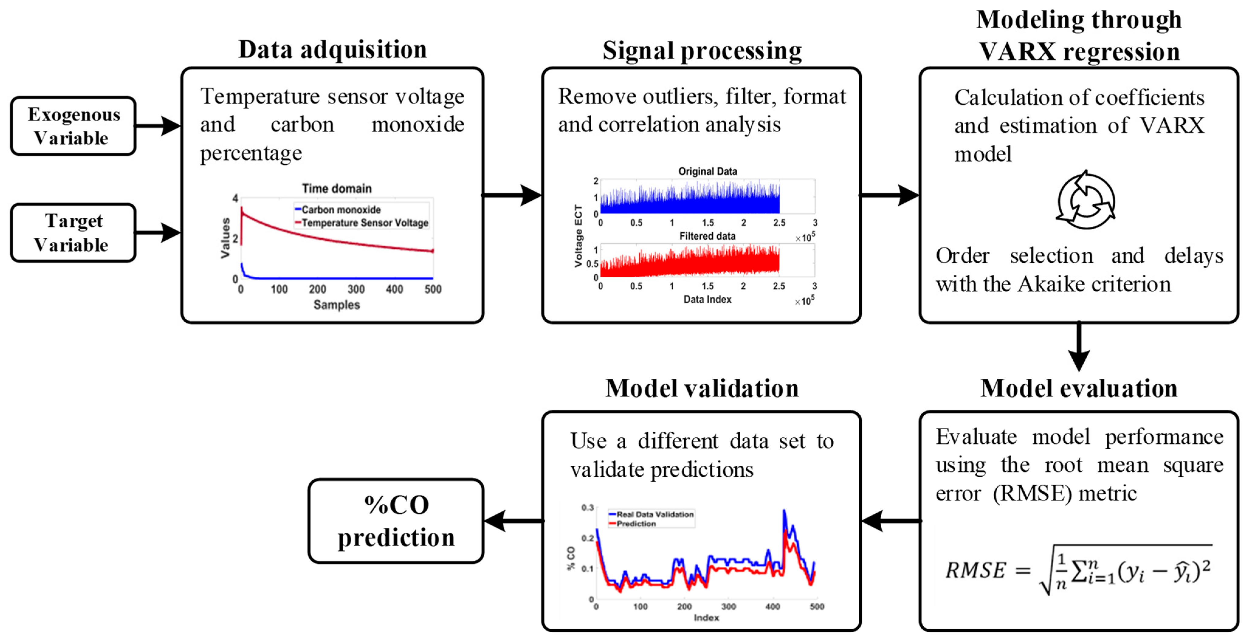
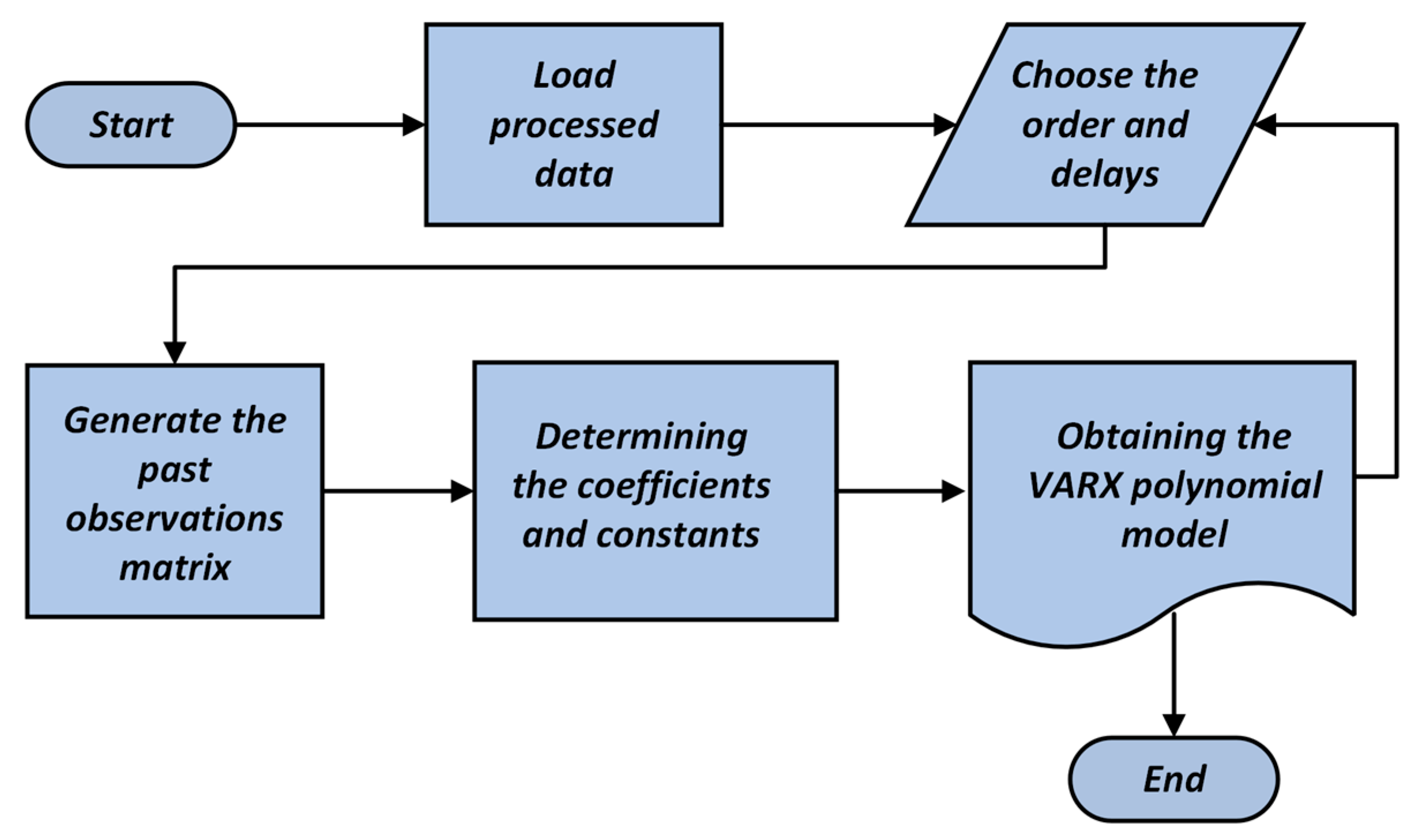
The proposed methodology applied to the analysis and modeling of CO in an ICE consists of four main steps as depicted in the flow chart of Figure 1. The goal of this work lies in applying the technique of temporal autoregressions to obtain a mathematical model capable of predicting CO emissions as a function of the engine temperature. Thus, the proposed method is carried out through the following steps: (i) data acquisition, (ii) signal processing, (iii) modeling through autoregression with exogenous variables (VARX), (iv) model evaluation, and (v) model validation; the details of each considered stage are described below.

3.1. Data Acquisition

The first stage is focused on the acquisition of data from different experimental tests; hence, it should be highlighted that the proposed modeling is supported by the use of signals that are measured from a vehicle’s engine, in this sense, in the first stage they are measured the engine temperature and the CO emissions. The temperature signal is acquired from the engine coolant temperature (ECT) sensor and the CO emissions are acquired from the vehicle exhaust pipe. Both signals are continuously measured and acquired for 500 s (approximately 8 min) of the start-up of the vehicle’s engine, that is, the signals are recorded from an initial temperature value (ambient temperature) until the vehicle’s engine reaches its normal operating temperature considered as the thermal steady state (approximately between 95 °C and 100 °C). These signals are stored in a personal computer for further analysis.

3.2. Signal Processing

Once the data acquisition is carried out, the second stage is achieved the processing of the acquired signals (ECT signal and CO emissions), and this stage is applied with the aim of analyzing the correlation between signals, and also to analyze data distribution for identifying unusual patterns (outliers). In this regard, the analysis of data distribution is carried out by means of scatter plots, whereas the correlation between variables is calculated through the Pearson and Spearman correlation coefficient, which allows us to understand the relationships between both acquired signals and leads us to determine the strength and direction of the associations, as well as the monotonic relationship between the studied variables. The Pearson and Spearman correlation coefficients are calculated using Equations (4) and (5), respectively [25].

$$r=\frac{{\sum }_{i=1}^n\left(X_i-\overline{X}\right)(Y_i-\overline{Y})}{\sqrt{{\sum }_{i=1}^n{\left(X_i-\overline{X}\right)}^2}\sqrt{{\sum }_{i=1}^n{\left(Y_i-\overline{Y}\right)}^2}}$$

(4)

where n is the number of observations, $X_i$ and $Y_i$ are the values of the variable $X$ and $Y$, respectively, in the i-th observation, and ${\overline{X}}_i$ and ${\overline{Y}}_i$ are the means of the variables $X$ and $Y$, respectively.

$$\rho =1-\frac{6\sum {d_i}^2}{n\left(n^2-1\right)}$$

(5)

where n is the number of observations and $d_i$ is the difference between the ranks of the observations i of the two variables.

On the other hand, descriptive statistics are used to detect whether outliers are the result of errors, incorrect data, or spurious fluctuations that do not represent the true dynamics of the system. Techniques for modeling systems using time series such as VARX models can become overly complex and prone to overfitting if fitted to noisy or unsmoothed data. By filtering and smoothing the data, the complexity of the model can be reduced and its predictive capacity improved [26]. That is why low-pass filtering and moving average filtering are considered to smooth the data, thus eliminating or reducing this noise, allowing the model to focus on significant relationships between variables. Additionally, appropriate encodings are applied to binary data. Finally, in order to evaluate the performance of the proposed modeling, the processed data are then divided into two different datasets, the first one considered for training and the second one used for the evaluation.

3.3. Modeling through VARX Regression

The modeling of CO emissions in terms of the ECT temperature is accomplished in the third stage, such modeling is performed through a VARX regression, and it is applied to the data processed in the previous stage. In Figure 2 shows the flow chart of the pseudocode that is implemented under GNU Octave for obtaining the mathematical model, the steps considered in the pseudocode of Figure 2 are as described below.

(i)

Start: in this section, the initial setup of the program is performed by cleaning the command and graphic windows, and a timer is started to measure the execution time of the code.

(ii)

Load processed data: In this part, the data from the experiments are loaded from the .txt files. The data are assigned to the output ($Y$) and input ($X$) variables, and additionally, in this stage, the loaded data are divided into two segments where one of the first parts is used for training purposes and the second one is used for validation. Additionally, a conversion of the coolant sensor data from binary to analog is performed to visualize them in voltages.

(iii)

Choose the order and delays: The order of the VARX model is defined for the output variable (p) and for the input variable (q), according to Equation (3). These values determine the number of past observations that will be considered in the model.

(iv)

Generate the past observations matrix: Lag matrices (Ylag and Xlag) are constructed, representing past observations of the output and input variables, respectively. Initial rows containing invalid values introduced by the lag matrix are then removed. These matrices are then used to capture the temporal dependence between the variables.

(v)

Determining the coefficients and constants: In this process, an algorithm is utilized to estimate the coefficients of the VARX model (coefficients of the design matrix) through linear regression, employing the least squares method as depicted in Equation (6) [27]. This equation is expressed in matrix form, and $\beta$ is found by solving the system of equations using the GNU Octave (v9.1) operator. Finally, the coefficients of the design matrix are separated into constants (c), coefficients of past observations of the output variable ($\phi$), and coefficients of past observations of the input variable (b).

$$E\left({\phi }_{0,}{\phi }_1,\dots {\phi }_m\right)=\sum _{i=1}^n{\left(y_i-f\left(x_i\right)\right)}^2$$

(6)

where $E({\phi }_0,{\phi }_1,\dots {\phi }_m)$ is the squared error function, representing the squared difference between the actual values y_i and the values estimated by the function $f\left(x_i\right)$ for each data point. $Y_i$ is the dependent variable, the output, or the observed value corresponding to data point i. ${\phi }_0$, ${\phi }_1$, and ${\phi }_m$ are the coefficients of the polynomial function determined to minimize the squared error, and $f\left(x_i\right)$ represents the function sought to approximate the data.

(vi)

Obtaining the VARX polynomial model: predictions are made using the estimated coefficients and the data design matrix. The model obtained in the process is pre-evaluated using the Akaike criterion as shown in Equation (7); subsequently, the order is adjusted, and another alternative model is obtained through the same process. This metric is used to compare three alternative models to determine in which of them the order of delays in the input (exogenous) and output variables was appropriate; a low value compared to alternative models indicates better performance [28].

$$AIC=-2\mathit{log}\left(L\right)+2(p+q)$$

(7)

where L is the likelihood function of the estimated model, p is the number of lags in the VARX model, and q is the number of lags of the exogenous variables.

3.4. Model Evaluation

In the model evaluation process, the error is estimated using the Root Mean Square Error ($RMSE$) metric, which provides a quantitative measure of the discrepancy between the values predicted by the model and the actual observed values. Estimating the error ensures the robustness and accuracy of the developed model, allowing for a clearer understanding of its performance and predictive ability. $RMSE$ is used as a standard statistical metric to measure the performance of the obtained model; in fact, this metric has been used in different research fields such as meteorology, air quality, and climate research studies because its use as an optimal metric for detecting normal (Gaussian) errors has been demonstrated. Therefore, the calculation of the square root does not affect the relative rankings of the models, but it yields a metric with the same units as y, conveniently representing the typical or “standard” error for normally distributed errors. The calculation of $RMSE$ is carried out using Equation (8).

$$RMSE=\sqrt{\frac{1}{n}{\sum }_{i=1}^n{(y_i-\widehat{y_i})}^2}$$

(8)

where n is the number of observations, y_i are the actual values, and ŷ_i are the predictions.

Using this metric is convenient if the goal is to have a measure of error on the same scale as the original data for a more intuitive interpretation and if large errors are critical. However, it is important to consider the advantages and disadvantages described below. Advantages: It is on the same scale as the original data since it takes the square root of the MSE, facilitating interpretation and direct comparison with the original values. Like MSE, it heavily penalizes large errors. Disadvantages: it may give less weight to large errors compared to MSE, as the square root smooths the effect of squares [29].

3.5. Model Validation

To validate the model, a new set of acquired test data (validation data) is used. Essentially, the procedure is like the previously described evaluation steps. A new test prediction is made by multiplying the design matrix of the new dataset, but this time with the coefficient matrix obtained from the original model; that is, the coefficients of the evaluated model are used with the design matrix of the new dataset (validation data). Subsequently, the performance of the specific VARX model is determined again using the $RMSE$ criterion as described in the previous step. To reinforce the validation, an equivalent model is obtained using simulation with GNU Octave with the same training and validation data to compare it with another alternative model. Since simulation using GNU Octave evaluates performance with the “Fit to Estimation Data” (FED) criterion, this same criterion is used to ensure the adequacy of the evaluation of the proposed model. The FED refers to a measure of how well a model fits the training data and is based on the calculation of variance [30]. In this section, to calculate it as a percentage, model predictions are compared with actual data, and the percentage of variance in the actual data determined by the model predictions is calculated. To do this, using the GNU Octave script developed, the total variance is calculated as shown in Equation (9), then the residual variance is calculated according to Equation (10), and finally, the Fit to Estimation Data are obtained using Equation (11).

$$Totalvariance=\frac{1}{n}{\sum }_{i=1}^n{\left(y_i-{\overline{y}}_i\right)}^2$$

(9)

$$Residualvariance=\frac{1}{n}{\sum }_{i=1}^n{\left({Residual}_i\right)}^2$$

(10)

$$Fittoestimationdata=\left(1-\frac{residualvariance}{totalvariance}\right)\ast 100$$

(11)

where n is the number of observations, y_i is the actual value in observation i, and ${\overline{y}}_i$ is the mean of the actual values and Residual_i = actual values − predictions in the observation i.

4. Experimental Setup

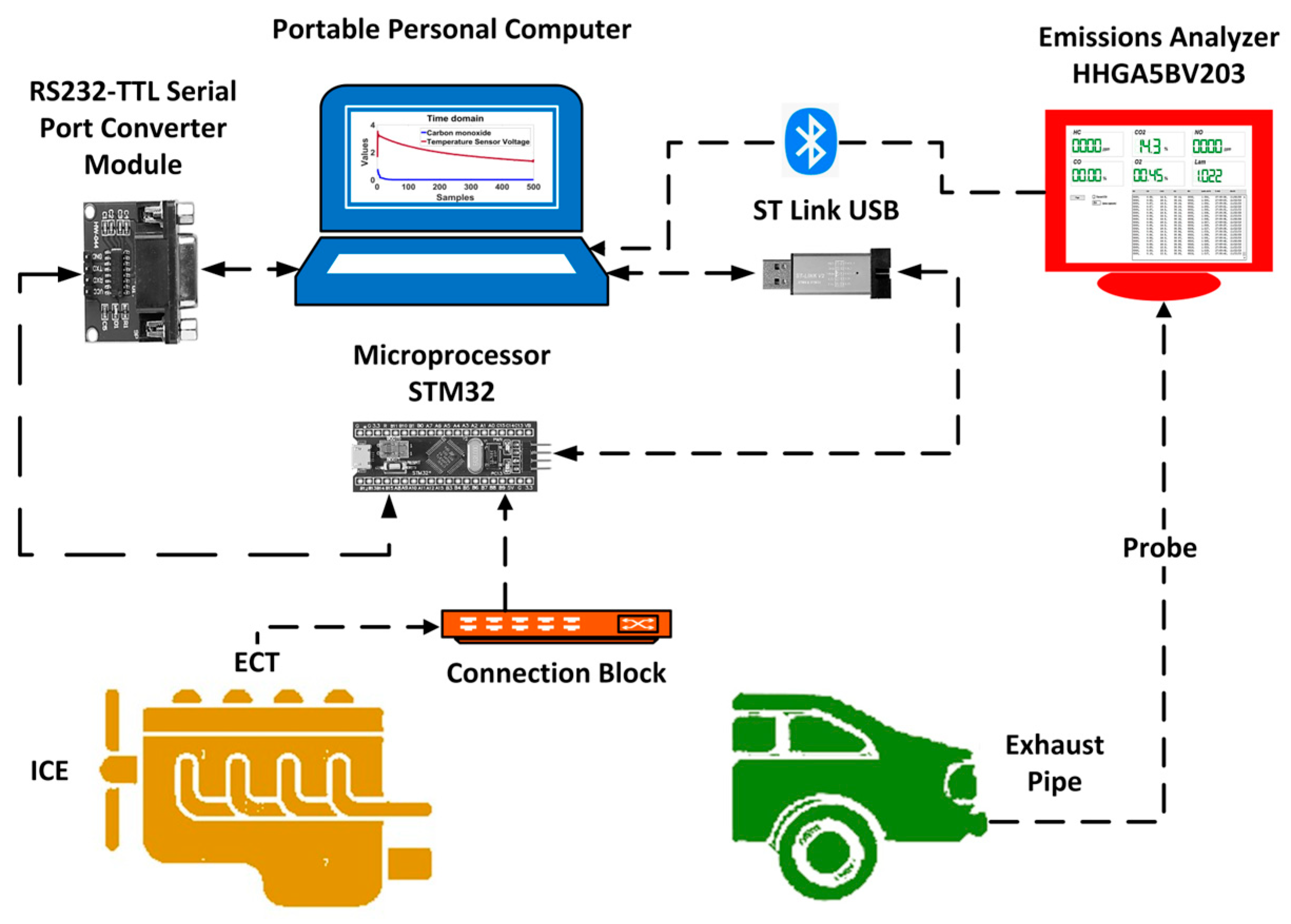
The proposed methodology is applied to experimental data acquired from a vehicle’s engine, the acquired data belong to the engine coolant temperature (ECT) sensor, which is considered the exogenous variable, and the carbon monoxide (CO) emitted by the vehicle’s exhaust pipe is used as the output variable. Figure 3 shows a schematic of the test bench, which is composed of seven components described below. The technical data of the vehicle and the engine operating temperature ranges used for the experiments are shown in

Table 2. Technical data of the test vehicle including the cooling system temperature ranges.

Vehicle Class	Suburban
Manufacture	Honda
Model line	CR-V
Subline	LX 4X4
Manufacture Year	2012
Engine displacement	2.4 L
Thermostat begins to open	76 °C to 80 °C
Thermostat fully open	90 °C
Operating temperature threshold	95 °C to 100 °C

.

Prior to testing, the vehicle was mechanically and electronically inspected to ensure that its operation is under normal conditions during the test. The vehicle’s engine is equipped with a junction box enabled with three ports to extract the signal from three sensors; in this case, only the ECT signal is used. The acquisition of the ECT signals is carried out by a STM32F411 microcontroller through a 12-bit analog-to-digital converter, and according to the specifications of these factors, conditioning was applied to the ECT voltage signal, which delivers 0 to 5 V DC. Thus, using a voltage divider, the microcontroller receives 0 to 3.3 V DC. While the CO emissions are acquired by using a gas analyzer device model HHGA5BV203, these signals are acquired with sampling frequencies equal to 1 kHz. Different tests are performed under static conditions, that is, the signals are monitored and acquired at 750 rpm (idle revolutions) and consist of starting the vehicle’s engine from its ambient temperature until the thermal operation of the vehicle’s engine reaches the thermal steady state (approximately between 95 °C and 100 °C). The idle revolutions are monitored using a scanning tool connected to the vehicle’s second-generation onboard diagnostic (OBD II) port. Thus, such testing takes approximately 10 to 15 min depending on the initial temperature, and given its nature, only three different experiments are conducted, but it is sufficient to consider that the samples obtained are representative of the studied phenomenon. A laptop computer with a 13th Gen Intel(R) Core (TM) i7-13650HX 2.60 GHz 64-bit processor and 16 GB of RAM is used to receive and store the acquired data and subsequently process the database. The experiment begins by starting the vehicle’s engine while simultaneously initiating the capture of ECT voltage data and CO percentage samples; once each experiment is completed, the acquired data are saved for subsequent analysis and processing.

5. Results and Discussion

This work proposes the development of a mathematical model by a linear autoregression with exogenous variables capable of predicting the behavior of CO emissions depending on one or more future samples of the engine temperature. Regarding the proposed methodology, the ECT signal and CO emissions are acquired from different experimental tests, the acquisitions are stored in a personal computer, then, the analysis and processing of data is carried out under the GNU Octave. As aforementioned, the acquired signals are divided into training and validation data, then, from each one of these two data groups the ECT signal is defined as the exogenous variable (the input to the algorithm) and the CO emissions signal is defined as the output variable. Accordingly, a preliminary analysis over the ECT and CO signals in the cold start test at idle speed is performed in order to interpret and understand the behavior of the data for the exogenous variable and the output variable. Thereby, Figure 4a,b show the graphical representation of the signals used during the training and validation procedure, respectively. The behavior of CO% observed in Figure 4a depicts a downward trend as samples are acquired, this trend means that the CO% decreases over time as the ECT voltage decreases, while the engine temperature increases to its normal operating temperature, from 95 °C to 100 °C. The ECT sensor is of thermistor type, so its behavior is normal for automotive applications; the reference voltage signal will be lower as the temperature increases. It is notable that after the 30th second, the CO stabilizes, indicating that both emissions control and the settling of the mechanical parts of the engine have begun to operate normally. On the other hand, Figure 4b shows the acquired signals that are used during the validation of the obtained model. In this one, the same downward trend in the decrease in the ECT voltage over time is observed, but there is a particular difference in the behavior of the CO percentage; in this case, it does not stabilize completely across the samples. However, this is a normal effect that may be due to internal mechanical conditions of the engine, such as wear on rings or valves, for example, and sometimes they do not always work ideally during cold starts. Nonetheless, the CO percentage in both experimental tests tends to be below 0.5% CO as the engine temperature reaches its optimal levels. Hence, it should be highlighted that the acquired signals presented in Figure 4a,b belong to acquisition obtained from different experiments; in this sense, in the rest of the manuscript the terms of training data and validation data may refer to the acquired data used for training and validation.

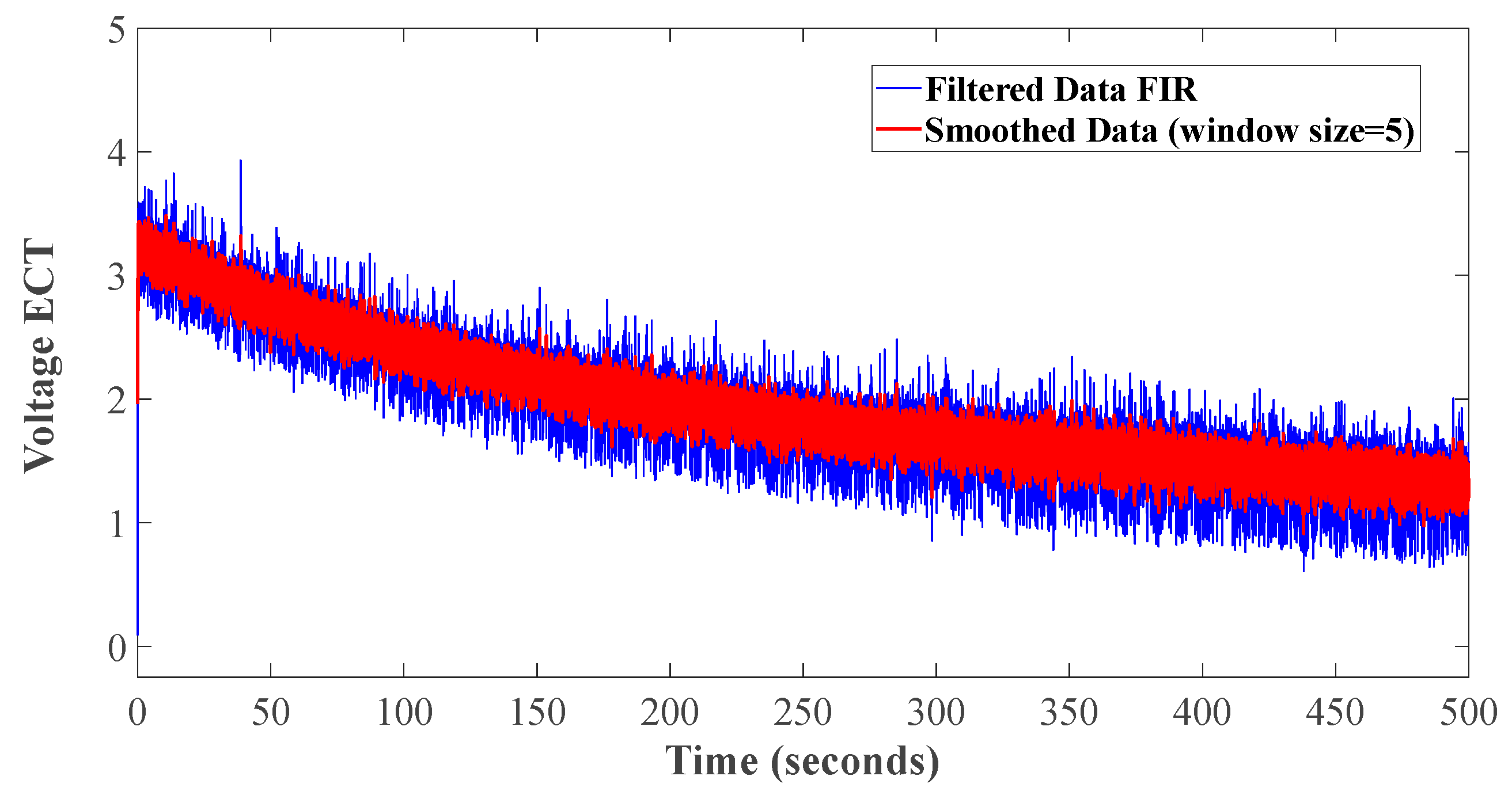
From the data obtained in Figure 4a (training data) and by applying the digital low-pass filter or “Finite Impulse Response-FIR” filter, a visual representation was obtained to project the original signal and the filtered signal as shown in Figure 5a,b. The impulse response is designed to attenuate or eliminate the high-frequency components of the ECT signal as shown in Figure 5a, while allowing the low-frequency components to pass and only respond to a finite number of input samples. In this case, the desired frequency response is specified, and then the window design algorithm is used to determine the filter coefficients that meet those specifications and achieve a satisfactory result as shown in Figure 5b. However, since this filter may not be fully effective in reducing outliers, a moving average filtering is also applied. The inclusion of this filter, in combination with a low-pass filter, provided a robust and effective strategy to attenuate outliers and improve the reliability of the signal of interest, as observed in Figure 6.

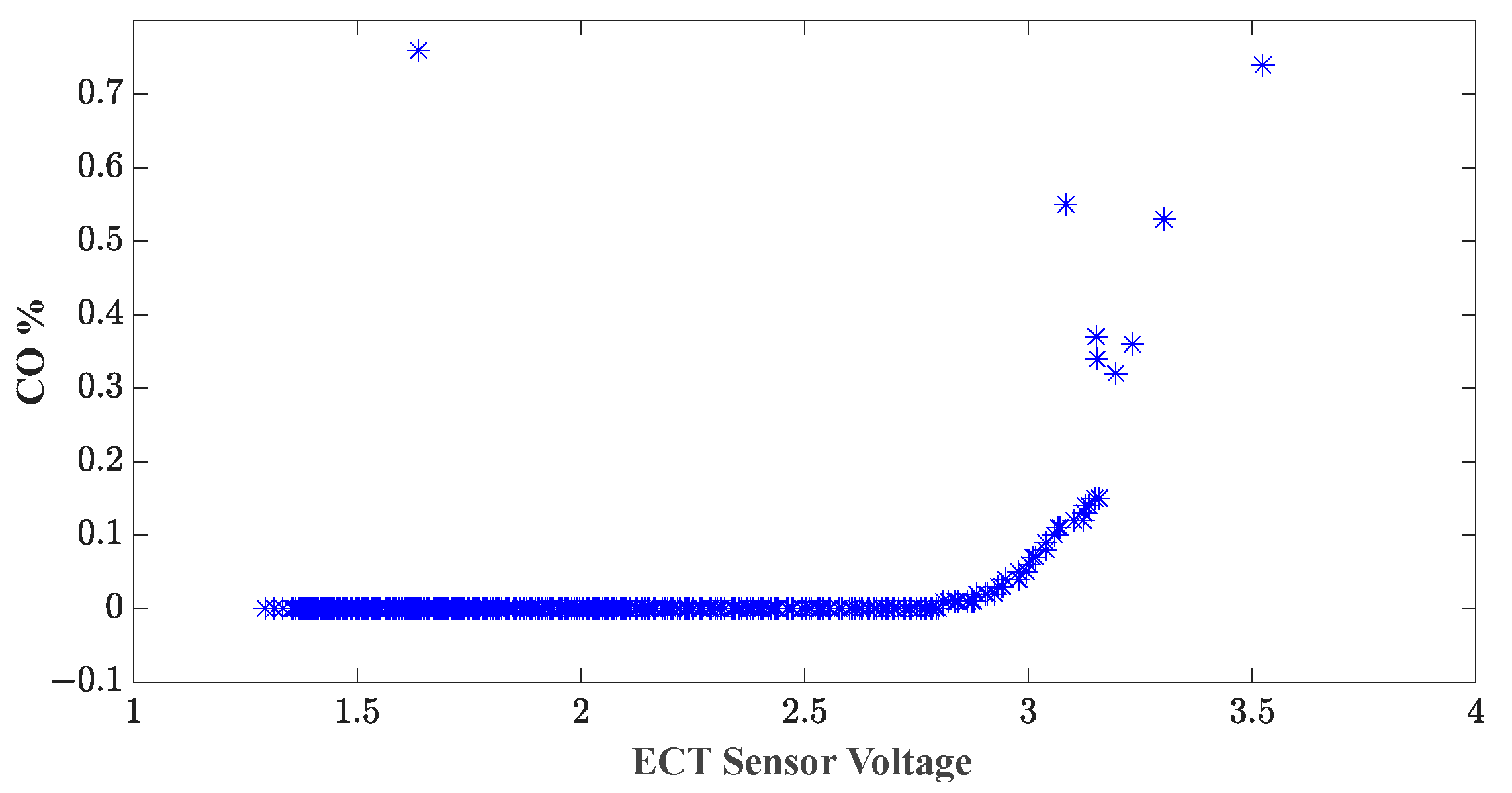
Moreover, the Spearman correlation coefficient is estimated in order to evaluate the correlation between acquired signals that belong to training data, and this estimated metric allows us to assess the monotonic relationship between variables. Thereby, the Spearman correlation coefficient estimated is around 0.48629; this value depicts a positive correlation between the assessed variables (ECT and CO) and suggests a clear connection that is less susceptible to anomalous influences, especially in scenarios with nonlinear data or outliers. This implies that as one set of data increases, the other tends to increase as well, and vice versa, with a clearer association. Therefore, the Spearman coefficient may be preferable when seeking more robust and clearer relationships between variables, especially in environments with complex or nonlinear data. Subsequently, to obtain a visual representation, a scatter plot was used between the ECT sensor voltage and the CO% from the cold start test, shown in Figure 7. In this scatter plot, it can be observed that when the ECT voltage remains in the range of 0 to 2.8 V, the CO% stays at a minimum. However, as the voltage increases from 2.8 to 3.6 V, the CO% increases considerably in an exponential manner. In practical terms, this means that the CO% remains high if the engine temperature is low, as the ECT voltage decreases as the engine temperature increases.

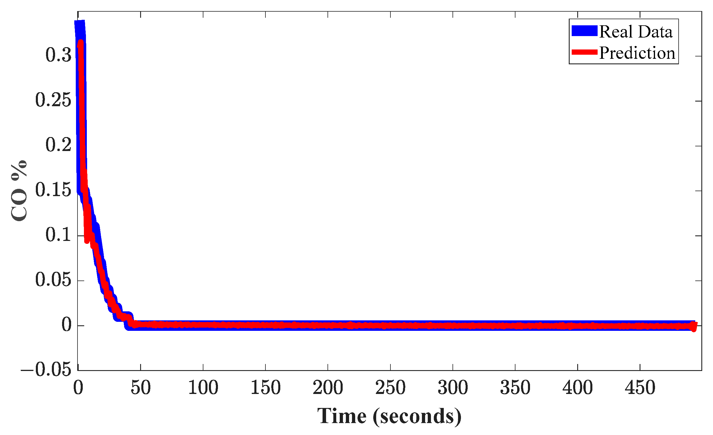
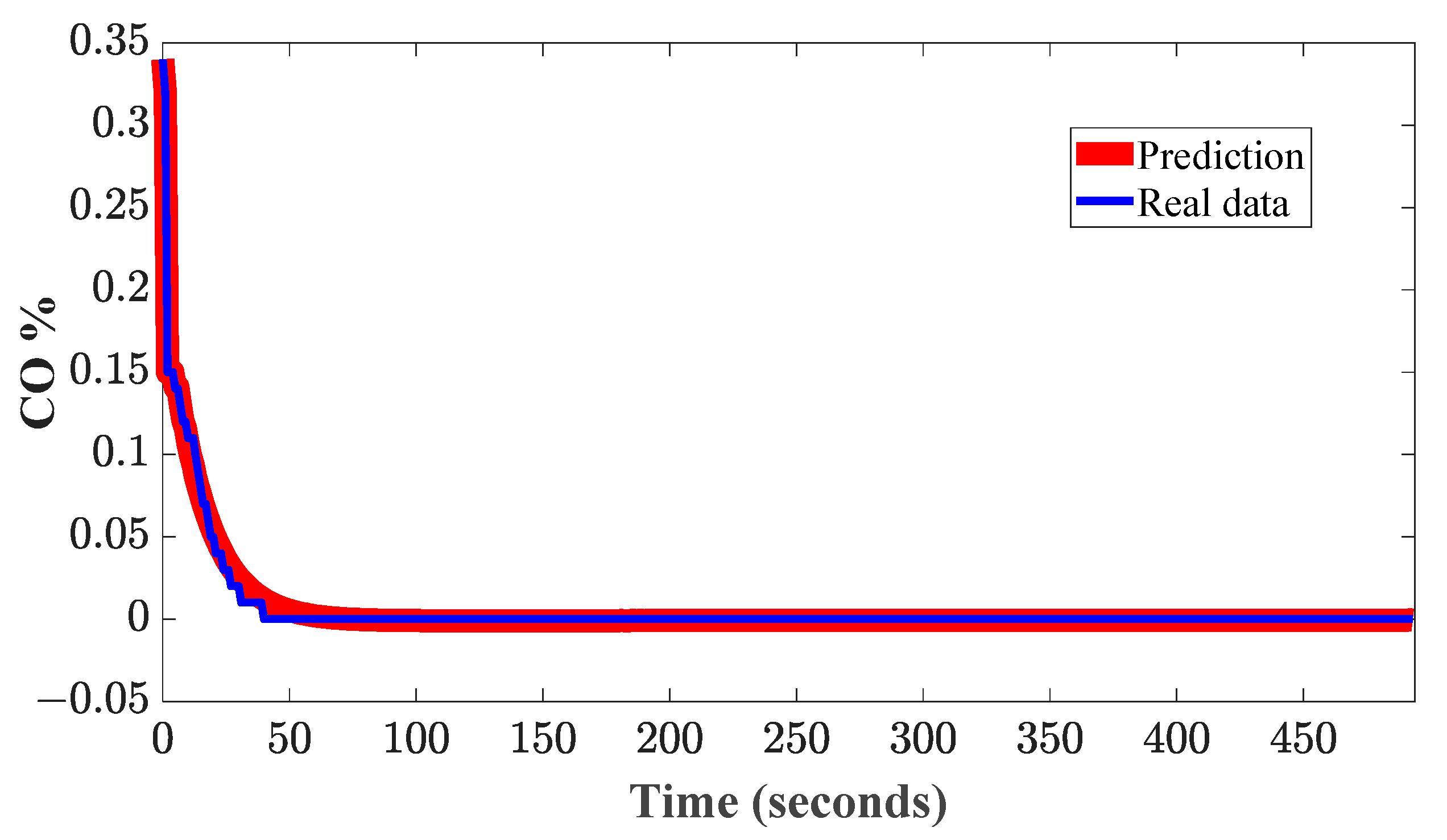
Accordingly, once the signals are processed, the development of the CO-ECT VARX emissions model is initiated as described in Section 3.3. For this purpose, the exogenous variables x(t) and the target variables y(t), which are the ECT voltage and CO% signals, respectively, are loaded into the program developed in GNU Octave. Consequently, seven models are obtained by selecting different orders in the delays of the input and output variables. For each execution, the matrix of past observations corresponding to training data, called the design matrix, is generated. Coefficients and constants are estimated using the least squares technique, and their components are separated. Subsequently, the model with its respective parameters was obtained and with the obtained VARX model, a graphical representation and a specific mathematically linearly adjusted model were developed for use in future sample projections. Figure 8a,b display the graph of the VARX model and a test prediction with the best of the models tested. Certainly, the prediction in Figure 8a is achieved by considering a 4-2 order modeling, whereas the prediction of Figure 8b is obtained by taking into account a 2-1 order modeling. For both predictions, we used the Akaike criterion, which resulted in about −3739.3, meanwhile, the $RMSE$ were about 0.0061061 and 0.0074449, respectively. On the other hand, Figure 9 presents the obtained graph of the best VARX model out of the three obtained under the $RMSE$ metric criterion, as it yielded a value of 0.0053971. As explained in Section 3.4, this criterion is used as a standard statistical metric to measure the performance of a model obtained, so it can be inferred that the performance of the CO-ECT VARX 6-3 model is better compared to the CO-ECT VARX 4-2 and CO-ECT VARX 2-1 models.

On the other hand, according to the general Equation (3) of a VARX model presented in Section 2.3, the programming of proposed modeling also generates the mathematical model in its sixth-order polynomial form of delays as observed in Equation (12). This model can represent the behavior of CO in a generic ICE during the transient cold start phase, within the temperature ranges of thermostat opening and closing as well as within the following:

$$\begin{array}{cc}\hfill Y\left(t\right)=-0.0023455& +0.75242\ast y\left(t-1\right)-0.28887\ast y\left(t-2\right)+0.16976\ast y\left(t-3\right)+0.2555\ast y\left(t-4\right)\hfill \\ & -0.23088\ast y\left(t-5\right)+0.11744\ast y\left(t-6\right)-0.029791\ast x\left(t-1\right)+0.051302\hfill \\ & \ast x\left(t-2\right)-0.020182\ast x\left(t-3\right)+\epsilon \left(t\right)\hfill \end{array}$$

(12)

where Y(t) represents the % of CO at time t, and −0.0023455 is a constant. The coefficients in the delays y(t − n) and x(t − n) are the autoregression coefficients of CO and ECT, respectively, indicating how past values influence Y(t), and ε(t) is the error term that captures the variability not explained by past values. The value of the Akaike information criterion (AIC), which was −3739.3, suggests an adequate model in terms of fit and simplicity compared to other alternative models calculated using the same autoregression strategy.

For evaluating the performance of the proposed model and in order to compare it with other approaches, the obtained model is compared with another similar model through simulation using the GNU Octave, where the same initial delay criteria were used. In Figure 10, the resulting model obtained through simulation is shown, which is very similar to the one obtained with the methodology proposed in this work. In this model, the FED was 96.4% with the training dataset, indicating that the model explains approximately 96.4% of the variability in the training data. A high value like this suggests that the model fits well with the training data and can capture the relationships between the input and output variables. However, using the Akaike criterion to evaluate the same simulation model again, with a value of around −10.07, it becomes evident that the modeling obtained through the proposed methodology is better than that of the simulation, as, according to this criterion, a lower magnitude indicates a better-fitting model. Accordingly, the use of this simulation tool has significant disadvantages compared to the model developed with the proposed methodology: (i) The functionalities available in GNU Octave are limited to the algorithms and methods included in the platform, which can restrict the flexibility and customization capability of the model. (ii) It may be subject to software version limitations, which can lead to additional costs and long-term compatibility issues. (iii) Depending on the level of detail provided by GNU Octave, users may have a less profound understanding of the structure and internal functioning of the model, which can hinder the interpretation of the results. (iv) There may be potential limitations in the metrics used to evaluate the model, either due to incompatibility with standard usage metrics or due to a lack of understanding of them. Similarly to the previous case, the simulation model through the GNU Octave has its respective sixth-order polynomial form, as shown in Equation (13), according to the equation of the VARX models presented in the theoretical section.

$$\begin{array}{cc}\hfill Y\left(t\right)=1-0.8309& \ast y\left(t-1\right)-0.02692\ast y\left(t-2\right)-0.3795\ast y\left(t-3\right)+0.3446\ast y\left(t-4\right)-0.06672\hfill \\ & \ast y\left(t-5\right)+0.01918\ast y\left(t-6\right)-0.0008661\ast x\left(t-1\right)+0.001309\ast x\left(t-2\right)\hfill \\ & -0.0004185\ast x\left(t-3\right)+\epsilon \left(t\right)\hfill \end{array}$$

(13)

To quantify the accuracy of the obtained models, the error was estimated using the $RMSE$ metric, which is commonly employed in predictive model evaluation. In this vein, the performance of the model obtained with the proposed methodology (Equation (12)) was compared to the model obtained by simulation (Equation (13)), using $RMSE$ as the evaluation metric, as detailed in Section 3.4 “model evaluation”. This criterion allowed for analyzing the performance of both models using the corresponding training data for each. As a result, an $RMSE$ metric of 0.0053971 was obtained for the developed VARX model, while for the simulation model, a value of 0.0010756 was recorded. This evaluation suggests that the simulation model might be better; however, in addition to the disadvantages of this simulation-based model mentioned earlier, the model using the proposed technique has the following advantages: (i) There is complete control over all stages of the process, from variable selection to model specification and interpretation of results. (ii) There is flexibility to adjust and modify the model according to specific problem needs and data characteristics, allowing for a more precise adaptation to study-specific conditions. (iii) With the suggested methodology, deeper insight into the model’s structure and functioning is gained, facilitating result interpretation and identification of potential issues or limitations. (iv) You are not limited by the functionalities available in a specific software tool, allowing for the implementation of customized techniques as needed. Additionally,

Table 3. Results of Akaike and $RMSE$ metrics of different alternative autoregression method models and the simulation model.

Types of ARX Models	Akaike Criterion	$\mathit{R}\mathit{M}\mathit{S}\mathit{E}$ Criterion
VARX 6-3 model developed	−3739.3	0.0053971
VARX 4-2 model developed	−3638.0	0.0061061
VARX 2-1 model developed	−3461.3	0.0074449
ARX 6-3 model simulated	−10.07	0.0010756

shows the comparative metric results of the alternative models using the proposed method and the model obtained by simulation. The values in Table 3 demonstrate a better performance of the developed VARX 6-3 model compared to the simulated ARX 6-3 model under the AIC criterion.

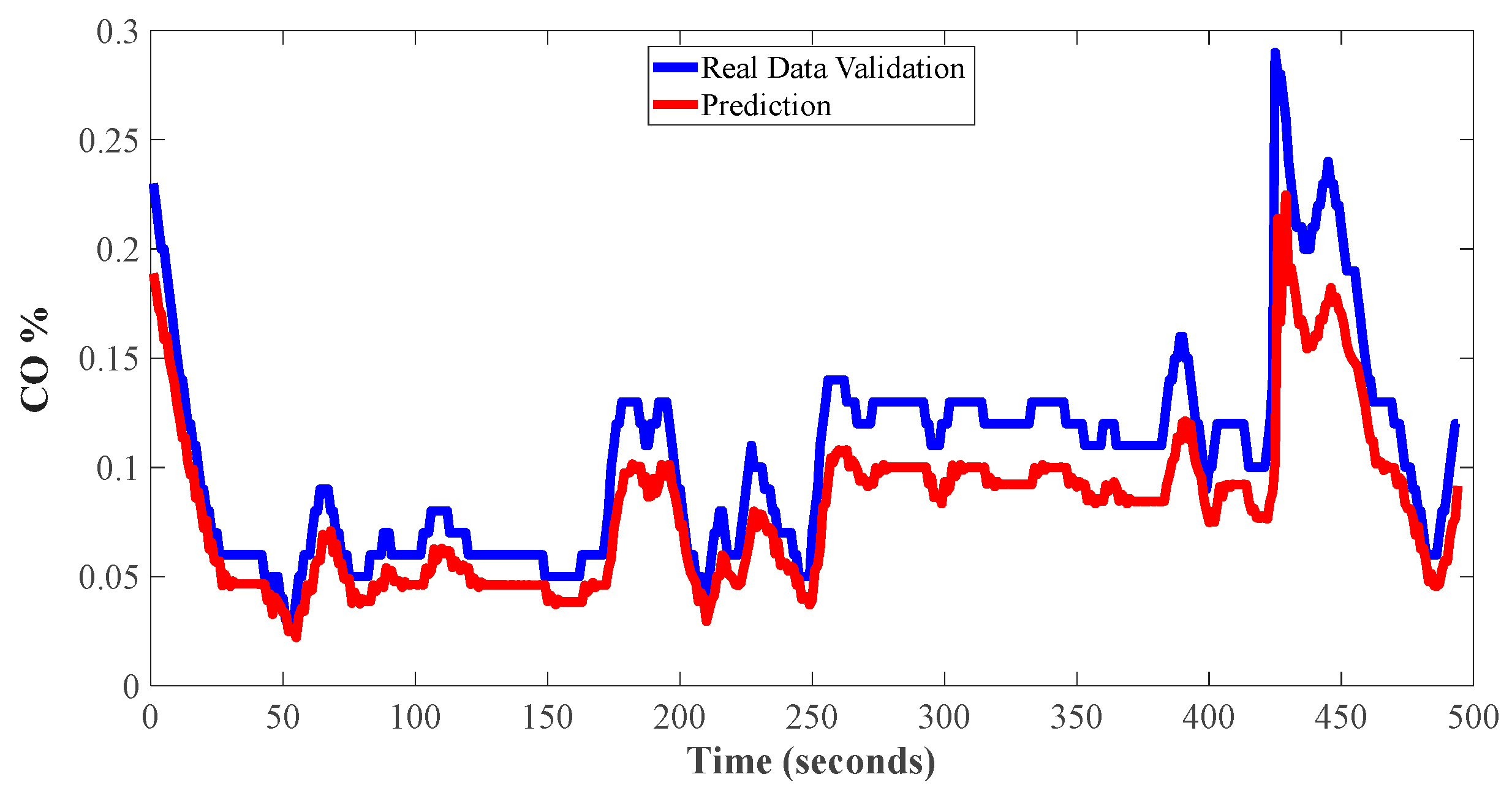
To validate the methodology of this work, the data from a new set of 500 samples of CO and ECT from the ICE obtained from training experimental data of the cold start idle speed test are used as input variables. The graph shown in Figure 11 represents the response of the CO VARX model obtained using the proposed methodology to a new set of data. This image demonstrates the model’s ability to respond to unknown data, and it is worth noting that the difference in signal patterns between training experiment data and validation experimental data is a normal condition, as emissions may increase slightly over time during ICE operation at idle speed due to various causes, such as the deformation of mechanical components like piston rings or valves due to temperature, which can affect cylinder sealing and combustion efficiency, as well as the ignition system, such as spark plugs, coils, or wires, which may exhibit differences in performance during the ICE cold start test.

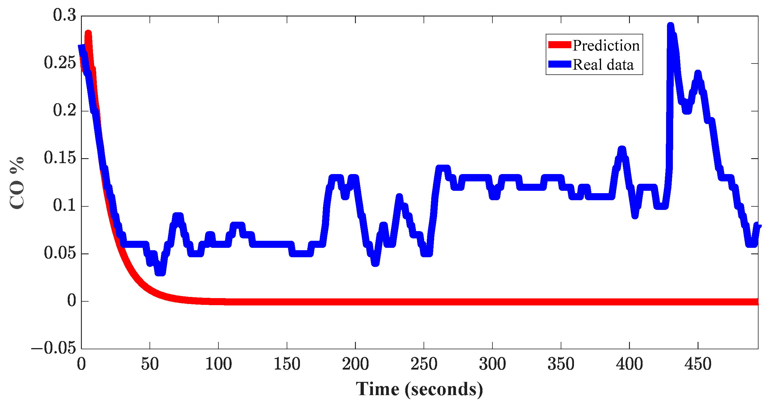
Although Figure 11 serves as a reference to observe the behavior of the proposed model with unknown values, it is necessary to analyze the information provided by the additional metric proposed in the Methodology section. The negative FED in the training dataset (−73.2%) suggests that the model has a narrow-range fit, meaning it may have captured too many idiosyncrasies in the training data. The negative value is not physically significant in this context; it only indicates overfitting. On the other hand, the positive FED in the validation dataset (90.6%) indicates that the model fits well with new data. This suggests that the model generalizes well to data it has not seen before, which is a positive sign that the model may have good predictive ability on new and unknown data. To test the CO-ECT ARX model obtained through simulation and provide a second comparative criterion with respect to the VARX 6-3 CO-ECT model obtained with the proposed method, new data obtained from experiment two of the same cold start test were used. Figure 12 depicts the graph illustrating the behavior of the simulated alternative model with a set of new data. The FED of −121.5% indicates that the simulation model fails to explain any variability with the new data for validation. This could suggest that this model does not generalize well to unknown data and fails to capture the underlying relationships between the variables in the validation dataset. Overall, such a significant discrepancy between the performance of the simulation model with the training data and the validation data signifies that it is overfitting to the specific details of the training data and cannot generalize correctly to new data.

The VARX 6-3 CO-ECT model developed using the suggested methodology has a negative FED in the training dataset, indicating a narrow-range fit. However, despite indicating a narrow-range fit, its ability to generalize and fit well to new data makes it more reliable than the ARX 6-3 model obtained through polynomial regression estimation using GNU Octave, as shown in

Table 4. Results of Fit to Estimation Data metrics of autoregression method model and the simulation model with the training dataset and validation dataset.

Types of ARX Models	Fit to Estimation Real Data	Fit to Estimation Validation Data
VARX 6-3 model developed	−73.2%	90.6%
ARX 6-3 model simulated	96.4%	−121.5%

. On the other hand, the ARX 6-3 model obtained through simulation has a high FED with the training data, suggesting a good fit to the data; however, in the validation dataset, it is negative, indicating that its performance is lower than that of the other model in question. The conclusion is that performance on unknown data is crucial in model evaluation, as successful predictions in previously unknown situations are required.

In order to further validate the proposed method, a comparative analysis was conducted with other established models commonly employed in similar research studies. For this purpose,

Table 5. Comparative analysis of the proposed method with VARX, LSTM, SSVARX, and FFNN models.

Types of Models	Benefits and Limitations	Metric Used
Vector auto-regressive with exogenous Inputs VARX 6-3 (this research)	* It describes all interactions of the model inputs. * Good understanding of the process dynamics. * Limited application in some processes.	$RMSE$ average: 0.0053971
[16] Long Short-Term Memory LSTM	* It accurately represents time series systems. * The numerous hyperparameters required dramatically affect the model’s performance.	$RMSE$ average: 0.0457
[18] Stationary Subspaces-Vector auto-regressive with exogenous SSVARX	* High computing speed. * Guaranteed solution in optimization systems. * Inadequate for highly nonlinear processes.	$RMSE$ average: 0.0482
[7] Feedforward neural network FFNN	* Capable of learning any function. * The model parameters do not provide any visualization of the process. * Training the system is computationally expensive.	$RMSE$ average: 0.0175
[31] Multi-Task Learning with Modal Feature Extraction	* It can simultaneously predict multiple targets. * Stability in the model’s performance across diverse situations. * Losses associated with multiple prediction tasks.	Mean Absolute Percentage Error (MAPE) <0.61%
[32] Temporal Lead-Lag Correlations	* Good representation of correlations. * Accuracy in predictions. * Fine-grained data collection is required.	Improved performance of 8 predictions $RMSE$0.227
[33] Federated Transformer Learning	* Provides security and privacy in the data. * Good handling of non-identically distributed unidentified data. * Implementation complexity and high computational resources.	Feature Skew 0.9321

has been included, showcasing the performance metrics of the proposed model alongside those of Long Short-Term Memory, Stationary Subspaces-Vector auto-regressive with exogenous, and Feedforward neural network models. By juxtaposing the results obtained from these various methodologies, a thorough evaluation of the effectiveness and robustness of the proposed approach is facilitated. This comparative analysis not only underscores the strengths of our method, but also provides valuable insights into its performance relative to other state-of-the-art models in the field.

6. Conclusions

This work proposes a comprehensive methodology to monitor and model carbon monoxide emissions through a mathematical model based on Auto-Regressive Exogenous, which is highly suitable for this particular case. There are three different aspects that must be highlighted. Firstly, the analysis of the cold start tests at idle speed revealed a significant correlation between the voltage of the ECT sensor and CO emissions. When the ECT voltage is maintained in a range of 0 to 2.8 V, the % of CO remains at a minimum. However, as this voltage increases from 2.8 to 3.6 V, the % of CO increases exponentially. This means that the % of CO remains high if the engine temperature is low, as the ECT voltage decreases as the engine temperature increases. Secondly, the Spearman correlation coefficient, which depicted a value around 0.48629, shows a positive correlation between the variables, suggesting a clear connection and little susceptibility to anomalous influences, especially in this scenario with nonlinear data or outliers. Furthermore, the implementation of a digital low-pass filter combined with a moving average filter proved to be a robust strategy to attenuate extreme values and improve the reliability of the signal of interest. Thirdly, the construction of the VARX model, based on input variables (ECT voltage) and output variables (CO%), provided a linearly adjusted mathematical representation. The evaluation of the developed CO-ECT 6-3 VARX model using AIC and $RMSE$ information criteria indicated a satisfactory fit and good predictive capability, supported by the low magnitude of the mean square error, compared to alternative models obtained using the same technique. Similarly, using the FED criterion, the CO-ECT 6-3 VARX model substantially outperformed the ARX 6-3 model obtained by simulation with GNU Octave, consolidating the validity and effectiveness of the developed methodology. Therefore, the obtained results make the proposed methodology suitable to be implemented for monitoring, analyzing, and modeling CO emissions with respect to the ECT sensor during the start-up in an ICE. For future research, the use of emerging techniques and methods of artificial intelligence, such as machine learning and deep learning, is contemplated in order to include a greater number of exogenous variables and further improve the prediction of CO, as well as the possibility of predicting the emission of other toxic gases such as HC, NOx, and greenhouse gases like $\mathrm{C}{\mathrm{O}}_2$.

References

1. Ukaogo, P.O.; Ewuzie, U.; Onwuka, C.V. Environmental pollution: Causes, effects, and the remedies. In Microorganisms for Sustainable Environment and Health; Elsevier: Amsterdam, The Netherlands, 2020; pp. 419–429. [Google Scholar] [CrossRef]
2. IEA. The Energy World Remains Fragile but Has Effective Ways to Improve Energy Security and Tackle Emissions. Available online: https://www.iea.org/reports/world-energy-outlook-2023/executive-summary (accessed on 30 March 2024).
3. Aslam, A.; Ibrahim, M.; Mahmood, A.; Mubashir, M.; Sipra, H.F.K.; Shahid, I.; Ramzan, S.; Latif, M.T.; Tahir, M.Y.; Show, P.L. Mitigation of particulate matters and integrated approach for carbon monoxide remediation in an urban environment. J. Environ. Chem. Eng. 2021, 9, 105546. [Google Scholar] [CrossRef]
4. Ogunkunle, O.; Ahmed, N.A. Overview of biodiesel combustion in mitigating the adverse impacts of engine emissions on the sustainable human–environment scenario. Sustainability 2021, 13, 5465. [Google Scholar] [CrossRef]
5. IEA. CO2 Emissions in 2022. USA. Available online: https://www.iea.org/reports/co2-emissions-in-2022 (accessed on 22 November 2023).
6. Maidi, A.; Rodionov, Y.V.; Shchegolkov, A.V. Mathematical Modeling of Thermo-Regulation of Fuel in Diesel Engines Ya-MZ238. Iraqi J. Agric. Sci. 2018, 49, 670–676. Available online: https://www.iasj.net/iasj/download/7c97ae7993e83463 (accessed on 30 March 2024).
7. Torres, E.; Romero, J.; Apolo, V.; Rivera, N.; Vacacela, J. Optimización del uso de Refrigerante para Disminuir la Emisión de Contaminantes en Motores de Combustión Interna. 2017. Available online: https://rte.espol.edu.ec/index.php/tecnologica/article/view/483 (accessed on 22 February 2024).
8. Bebkiewicz, K.; Chłopek, Z.; Sar, H.; Szczepański, K.; Zimakowska-laskowska, M. Influence of the thermal state of vehicle combustion engines on the results of the national inventory of pollutant emissions. Appl. Sci. 2021, 11, 9084. [Google Scholar] [CrossRef]
9. Tuttle, J.F.; Blackburn, L.D.; Andersson, K.; Powell, K.M. A systematic comparison of machine learning methods for modeling of dynamic processes applied to combustion emission rate modeling. Appl. Energy 2021, 292, 116886. [Google Scholar] [CrossRef]
10. Türe, Y.; Türe, C. An assessment of using Aluminum and Magnesium on CO2 emission in European passenger cars. J. Clean. Prod. 2020, 247, 119120. [Google Scholar] [CrossRef]
11. Deng, Y.; Feng, C.; E, J.; Wei, K.; Zhang, B.; Zhang, Z.; Han, D.; Zhao, X.; Xu, W. Performance enhancement of the gasoline engine hydrocarbon catchers for reducing hydrocarbon emission during the cold-start period. Energy 2019, 183, 869–879. [Google Scholar] [CrossRef]
12. Ye, L.; Xie, N.; Hu, A. A novel time-delay multivariate grey model for impact analysis of CO2 emissions from China’s transportation sectors. Appl. Math. Model. 2021, 91, 493–507. [Google Scholar] [CrossRef]
13. Amran, M.A.N.; Bakar, A.A.; Jalil, M.H.A.; Wahyu, M.U.; Gani, A.F.H.A. Simulation and modeling of two-level DC/DC boost converter using ARX, ARMAX, and OE model structures. Indones. J. Electr. Eng. Comput. Sci. 2020, 18, 1172–1179. [Google Scholar] [CrossRef]
14. Hanafi, D.; Huq, M.S.; Suid, M.S.; Fua’ad Rahmat, M. A quarter car ARX model identification based on real car test data. J. Telecommun. Electron. Comput. Eng. 2017, 9, 135–138. [Google Scholar]
15. Xu, B.; Lin, B. Carbon dioxide emissions reduction in China’s transport sector: A dynamic VAR (vector autoregression) approach. Energy 2015, 83, 486–495. [Google Scholar] [CrossRef]
16. Ma, J.; Xu, F.; Huang, K.; Huang, R. Improvement on the linear and nonlinear auto-regressive model for predicting the NOx emission of diesel engine. Neurocomputing 2016, 207, 150–164. [Google Scholar] [CrossRef]
17. Tang, T.Q.; Yi, Z.Y.; Lin, Q.F. Effects of signal light on the fuel consumption and emissions under car-following model. Phys. A Stat. Mech. Its Appl. 2017, 469, 200–205. [Google Scholar] [CrossRef]
18. Yu, Y.; Wang, Y.; Li, J.; Fu, M.; Shah, A.N.; He, C. A novel deep learning approach to predict the instantaneous NOxemissions from diesel engine. IEEE Access 2021, 9, 11002–11013. [Google Scholar] [CrossRef]
19. Li, Y.; Tang, G.; Du, J.; Zhou, N.; Zhao, Y.; Wu, T. Multilayer Perceptron Method to Estimate Real-World Fuel Consumption Rate of Light Duty Vehicles. IEEE Access 2019, 7, 63395–63402. [Google Scholar] [CrossRef]
20. Ding, P.; Jia, M.; Yan, X. Stationary subspaces-vector autoregressive with exogenous terms methodology for degradation trend estimation of rolling and slewing bearings. Mech. Syst. Signal Process. 2021, 150, 107293. [Google Scholar] [CrossRef]
21. Álvarez, J.; Callejón, I. Motores Alternativos de Combustión Interna; Edicions de la Universitat Politécnica de Catalunya: Barcelona, España, 2005; ISBN 84-8301-818-5. [Google Scholar]
22. Stubblefield, M. and Haynes, J.H. Fuel Injection 1986 Thru 1999, 2000th ed.; Haynes de Norte America: Thousand Oaks, CA, USA, 2000. [Google Scholar]
23. Houston, P.L. Chemical Kinetics and Reaction Dynamics; Dover Publications: Mineola, NY, USA, 2006. [Google Scholar]
24. Nicholson, W.B.; Matteson, D.S.; Bien, J. VARX-L: Structured regularization for large vector autoregressions with exogenous variables. Int. J. Forecast. 2017, 33, 627–651. [Google Scholar] [CrossRef]
25. Moore, D.S.; McCabe, G.P.; Craig, B.A. Introduction to the Practice of Statistics; Purdue University: West Lafayette, IN, USA; W. H. Freeman and Company: New York City, NY, USA, 2014; ISBN 10 1-4641-5893-2. [Google Scholar]
26. Shumway, R.H.; Stoffer, D.S. Time Series Analysis and Its Applications. In Springer Texts in Statistics; Springer International Publishing: Cham, Switzerland, 2017. [Google Scholar] [CrossRef]
27. Sheng-Guzman, G.Y. Estimación de Modelos de Series Temporales Multivariantes para la Predicción de la Demanda Electríca. Bachelor’s Thesis, Universidad Politécnica de Madrid, Madrid, Spain, 2016. Available online: https://oa.upm.es/ (accessed on 30 March 2024).
28. Anderson, D.R.; Burnham, K.P.; White, G.C. Comparison of Akaike information criterion and consistent Akaike information criterion for model selection and statistical inference from capture-recapture studies. J. Appl. Stat. 1998, 25, 263–282. [Google Scholar] [CrossRef]
29. Hodson, T.O. Root-mean-square error (RMSE) or mean absolute error (MAE): When to use them or not. Geosci. Model Dev. 2022, 15, 5481–5487. [Google Scholar] [CrossRef]
30. Salazar, C.; Castillo, S. Fundamentos Básicos de Estadística, 1st ed.; Universidad de Quindío: Armenia, Colombia, 2018; ISBN 978-9942-30-616-6. [Google Scholar]
31. Tan, M.; Hu, C.; Chen, J.; Wang, L.; Li, Z. Multi-node load forecasting based on multi-task learning with modal feature extraction. Eng. Appl. Artif. Intell. 2022, 112, 104856. [Google Scholar] [CrossRef]
32. Zhu, N.; Wang, Y.; Yuan, K.; Yan, J.; Li, Y.; Zhang, K. GGNet: A novel graph structure for power forecasting in renewable power plants considering temporal lead-lag correlations. Appl. Energy 2024, 364, 123194. [Google Scholar] [CrossRef]
33. Yitong, S.; Sen, L. FedPT-V2G_Security enhanced federated transformer learning for real-time. Appl. Energy 2024, 358, 122626. [Google Scholar] [CrossRef]
Figure 1. Flow chart of the proposed methodology for modeling and predicting carbon monoxide in an ICE during the start-up by means of a VARX regression.
Energies 17 02493 g001
Figure 2. Flow chart of the pseudocode that is implemented under the Octave environment to obtain a primary CO-ECT VARX model during the start-up of an ICE.
Energies 17 02493 g002
Figure 3. Scheme of the experimental bench for sampling ECT voltages and CO emissions from an internal combustion engine.
Energies 17 02493 g003
Figure 4. Graphical representation of the acquired signals, these signals are acquired from two different experiments and are used for (a) the training of the mathematical model and (b) the evaluation of the trained model. Both Figures represent the behavior of the CO percentage and the ECT sensor voltage.
Energies 17 02493 g004
Figure 5. Original ECT voltage signal extracted from experiment one, filtered using a digital low-pass filter. (a) Original data and (b) filtered data.
Energies 17 02493 g005
Figure 6. Scheme of the inclusion of a moving average filter in combination with the low-pass filter to attenuate extreme values.
Energies 17 02493 g006
Figure 7. Scatter plot between ECT sensor voltage variables and CO percentage showing the type of relationship.
Energies 17 02493 g007
Figure 8. Plot of two alternative VARX models of CO-ECT and prediction during cold start testing in an internal combustion engine, using data from experiment one. (a) The 4-2 order model with R M S E : 0.0061061 and (b) the 2-1 order model with R M S E : 0.0074449.
Energies 17 02493 g008
Figure 9. VARX graphical model of CO-ECT and prediction during the cold start test in an internal combustion engine with R M S E : 0.0053971, using the training data.
Energies 17 02493 g009
Figure 10. ARX graphical model of CO-ECT and prediction through simulation, during the cold start test in an internal combustion engine, using the training data.
Energies 17 02493 g010
Figure 11. CO-ECT VARX model prediction during the cold start test in an internal combustion engine with R M S E : 0.027546, using news data (validation experimental data).
Energies 17 02493 g011
Figure 12. Failed prediction by the CO-ECT ARX model obtained through simulation during the cold start test in an internal combustion engine, using new data (validation data).
Energies 17 02493 g012