FCS-MPC Based on Dimension Unification Cost Function

Abstract

Finite Control Set Model Predictive Control (FCS-MPC) has the ability to achieve multi-objective optimization, but there are still many challenges. The key to realizing multi-objective optimization in FCS-MPC lies in the design of the cost function. However, the different dimensions of penalty terms in the cost function often lead to difficulties in designing weighting coefficients. Incorrect weighting coefficients may result in truncation errors in calculations of DSPs and FPGAs, thereby affecting the algorithm’s control performance. Therefore, this article focuses on a system driving an induction motor with a three-level Neutral Point Clamped (NPC) inverter, and selects stator current and switching frequency as penalty terms in the cost function. An improved method is proposed to unify the dimensions of both penalty terms in the cost function. By unifying the dimensions of the penalty terms, a simple design of weighting coefficients can be achieved. Subsequently, to balance the inverter’s switching frequency and the dynamic response performance of the motor, a composite cost function is further proposed. Finally, the rationality of the proposed method is validated through simulation and experimental platforms.

1. Introduction

Finite Control Set Model Predictive Control (FCS-MPC) has gained widespread application in the fields of power electronics and power transmission, owing to its advantages in time-domain control, multi-objective optimization, and nonlinear processing [1,2,3]. Notably, the three-level Neutral Point Clamped (NPC) inverter finds extensive application in variable frequency speed control systems for medium-voltage high-power motors, attributed to its advantages including multiple output levels, low voltage withstand of switching devices during off states, and high efficiency [4]. Consequently, FCS-MPC based on NPC topology presents a novel approach for achieving high-performance control of induction motors [5], gradually emerging as a research trend in recent years.

Presently, research on FCS-MPC predominantly centers on two fronts: Model Predictive Torque Control (MPTC) and Model Predictive Current Control (MPCC). MPTC capitalizes on the principles of FCS-MPC while integrating the direct torque control (DTC) methodology. In MPTC, each sampling cycle involves leveraging the discrete mathematical model of the motor to forecast torque and magnetic flux. Through iterative optimization of the objective function, the optimal switch state is selected to achieve high-performance control of the motor [6,7]. In the context of motor speed regulation utilizing MPCC, the stator current serves as the direct optimization objective. Online optimization of the inverter switch state is performed based on predictive values and the predefined objective function, enabling direct output. Relative to MPTC, this approach minimizes current harmonics and demonstrates broad applicability across power converters and motor drives [8,9].

FCS-MPC stands as a distinct branch within the realm of MPC, distinguished by its ability to meticulously explore all switch states of the inverter and select the optimal switch state output based on a defined cost function, thereby offering rapid response dynamics and facilitating multi-objective optimization [10,11,12]. Although FCS-MPC has the ability to achieve multi-objective optimization, it still faces many challenges, such as designing the cost function and selecting weight coefficients [13]. Unreasonable cost function design may not achieve multi-objective optimization and instead lead to system control errors.

Taking the implementation of MPCC cost function design as an example, it usually only includes the current penalty term. In theory, adding a switching frequency penalty term to the cost function could optimize the switching frequency, but in reality, it is not that straightforward. The current and switching frequency terms in the cost function need to be quantified by weighting coefficients to penalize their significance. However, due to the different dimensional properties of penalty terms, introducing an appropriate parameter as a weighting coefficient becomes difficult. The dimensional inconsistency between the switching frequency and current prevents the direct selection of weighting coefficients. For example, the current error may only be in the mA level, while the number of switch actions may be a natural number greater than 0. Adding these two directly, due to their different orders of magnitude, the decisive factor will only be the switch frequency limit term. During the implementation of the controller, truncation errors in calculations of chips such as DSPs and FPGAs may lead to a decrease in control performance if weighting coefficients are improperly chosen, posing a risk of vector selection errors. In order to quantify the significance of penalty terms in the cost function, a model predictive control scheme with variable weighting coefficients is proposed in [14], where switching frequency serves as an additional term in the cost function, effectively reducing the switching losses of the matrix converter. In [15,16], a novel method for representing switching frequency is proposed. Unlike traditional methods, it uses the error between voltage vectors instead of the number of switch actions to limit the switching frequency, achieving favorable control effects. This also provides new ideas for designing a unified dimensional value function. In addition, the switching frequency and the common-mode voltage are selected as the control target [17]. Their control is converted into the limitation of the current ripple so that the control parameters have a clear physical meaning. However, for multi-objective FCS-MPC program designs, weighting coefficients are typically obtained through numerous experiments and continuous adjustments [18,19].

In the aforementioned literature, the weighting coefficients are derived from engineering experience [20]. Currently, there is limited mathematical derivation regarding the selection of weighting coefficients. Therefore, the design and optimization of weighting coefficients for cost functions with multiple constraints become challenging tasks. Overall, the selection and optimization of weighting coefficients for multi-constraint cost functions pose a significant challenge in the field.

Addressing the aforementioned issues, this paper presents a solution for the challenging task of designing weighting coefficients in the cost function of MPCC in the context of an NPC topology induction motor drive system, combined with the principles of FCS-MPC. A method is proposed to constrain the weighting coefficients of the switching frequency term in the cost function. Stator current and switching frequency are selected as penalty terms in the cost function, and their dimensional consistency is unified. This approach significantly reduces the difficulty of tuning the weighting coefficients for constraining the switching frequency term. Furthermore, considering the operating characteristics of induction motors under various conditions, a composite cost function is proposed, integrating the steady-state performance advantages of MPCC and the dynamic performance advantages of MPTC, thereby enhancing the dynamic response performance of model predictive current control. The remaining contents of this paper are as follows: Section 2 introduces the traditional model predictive current control method based on NPC three-level inverters. Section 3 presents the proposed cost function design method, deriving the dimensional consistency of current and switching frequency terms in the cost function, and then designing a composite cost function for different operating conditions of the motor. Section 4 validates the proposed method through simulation and experimentation. Finally, Section 5 concludes the paper.

2. Predictive Mode of a NPC Three-Level Inverter with Induction Motor Load

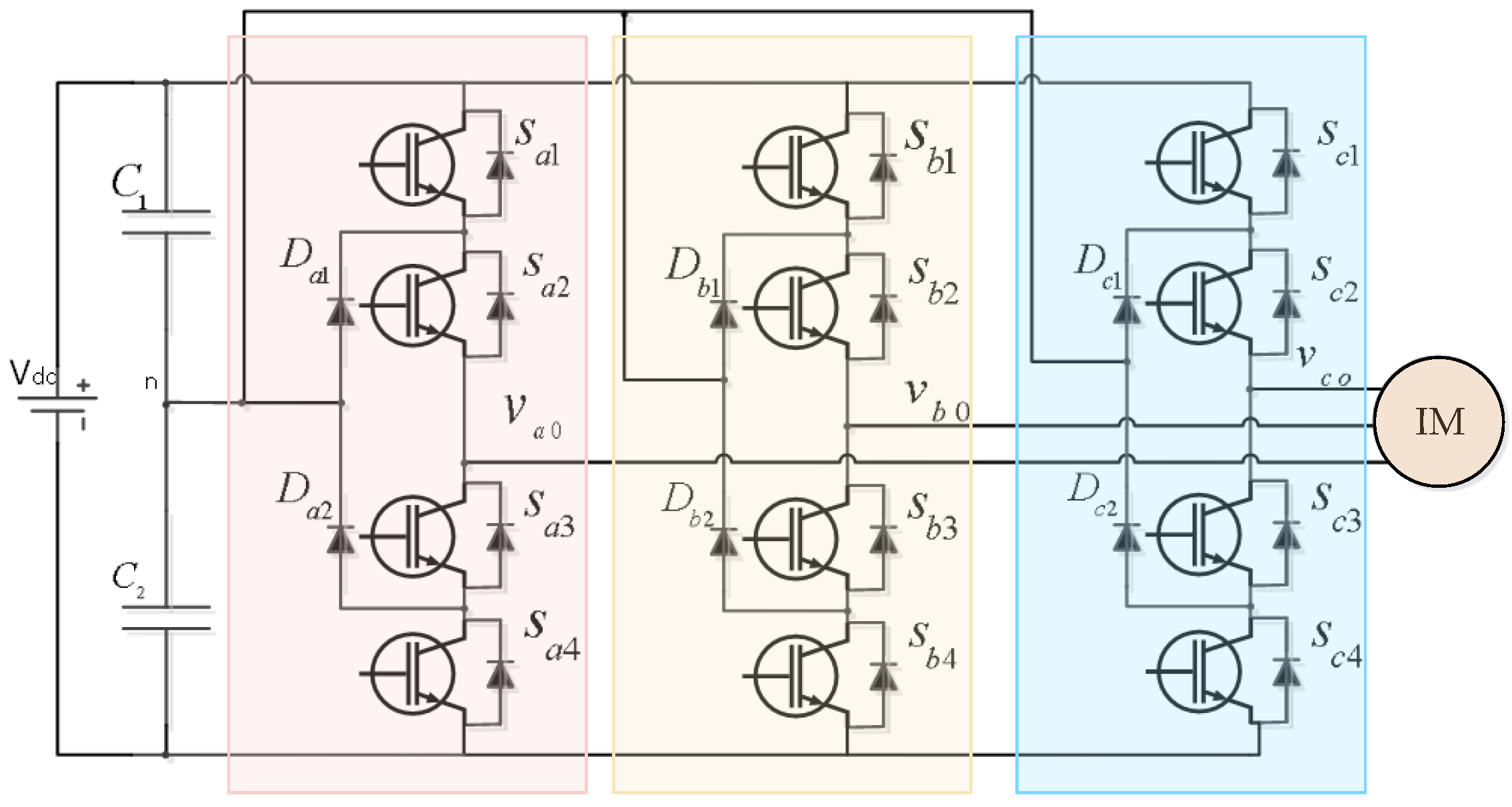
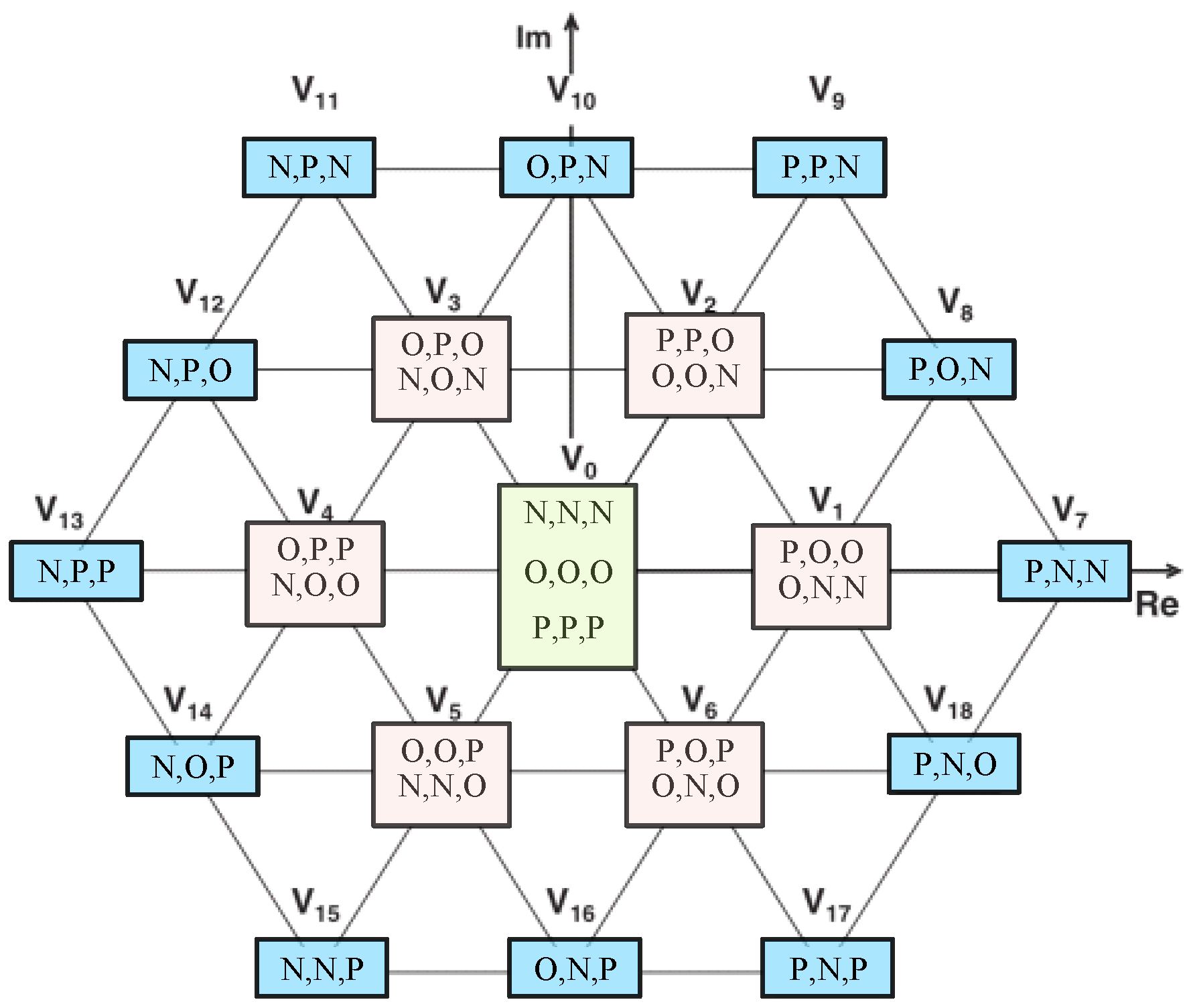
2.1. Mathematical Model of a NPC Three-Level Inverter

In Figure 1, V_dc represents the DC-link voltage, while C₁ and C₂ denote the DC bus capacitors. D_xy (where x = a, b, c and y = 1, 2) signifies the clamping diodes and S_xy (where x = a, b, c and y = 1, 2, 3, 4) denotes the power switches, which are IGBTs in this case. IM stands for the three-phase induction motor. Assuming all switches are ideal components and neglecting the forward conduction voltage drop of the switches, there are three operating states of each phase leg of the NPC inverter, taking the phase-a leg as an example:

(1)

State P: Switches S_a1 and S_a2 conduct simultaneously, while switches S_a3 and S_a4 are both off. In this state, V_ao = V_dc/2.

(2)

State O: Switches S_a2 and S_a3 conduct simultaneously, while switches S_a1 and S_a4 are both off. In this state, V_ao = 0.

(3)

State N: Switches S_a3 and S_a4 conduct simultaneously, while switches S_a1 and S_a2 are both off. In this state, V_ao = −V_dc/2.

In the normal operation of the NPC three-level inverter, defining the switch state variables S_a, S_b, and S_c to respectively represent the switch states of the phase-a, b, and c legs, the neutral point voltage of each phase can be expressed as (1):

$$v_{xo}=\frac{V_{\mathrm{dc}}}{2}{S}_x\hspace{1em}\hspace{1em}(x=a,b,c)$$

(1)

where the switch function S_x is defined as (2):

$$S_{\mathrm{x}}=\left\{\begin{array}{cc}1& “P”(S_{x1}, S_{x2}, S_{x3}, S_{x4})=(1,1,0,0)\\ 0& “O”(S_{x1}, S_{x2}, S_{x3}, S_{x4})=(0,1,1,0)\\ -1& “N”(S_{x1}, S_{x2}, S_{x3}, S_{x4})=(0,0,1,1)\end{array}\right.$$

(2)

and the inverter output voltage vector vs. can be derived as (3):

$$v_{\mathrm{s}}=\frac{2}{3}(v_{\mathrm{ao}}+a{v}_{\mathrm{bo}}+a^2{v}_{\mathrm{co}})$$

(3)

where $a=e^{j2\pi /3}=-1/2+j\sqrt{3}/2$, and there are 27 switch states, leading to 19 distinct voltage vectors, as illustrated in Figure 2.

Establishing the vector model of the induction motor, the stator current of the induction motor is represented on the complex plane as i_s, with its components on the α and β axes denoted as i_sα and i_sβ respectively. The voltage complex vector equation can be expressed as (4), and the flux complex vector equation is represented by (5):

$$\left\{\begin{array}{l}{\mathit{u}}_s=R_s{\mathit{i}}_s+\frac{d{\mathsf{\psi }}_s}{dt}\\ {\mathit{u}}_r=R_r{\mathit{i}}_r+\frac{d{\mathsf{\psi }}_r}{dt}\end{array}\right.$$

(4)

$$\left\{\begin{array}{l}{\mathsf{\psi }}_s=L_s{\mathit{i}}_s+L_m{\mathit{i}}_r\\ {\mathsf{\psi }}_r=L_m{\mathit{i}}_s+L_r{\mathit{i}}_r\end{array}\right.$$

(5)

Equations (4) and (5) depict u_s and u_r as the stator and rotor voltage complex vectors, i_s and i_r as the stator and rotor current complex vectors, Ψ_s and Ψ_r as the stator and rotor flux complex vectors, and R_s and R_r as the stator and rotor resistances, while L_s, L_r, and L_m represent the stator inductance, rotor inductance, and leakage inductance, respectively.

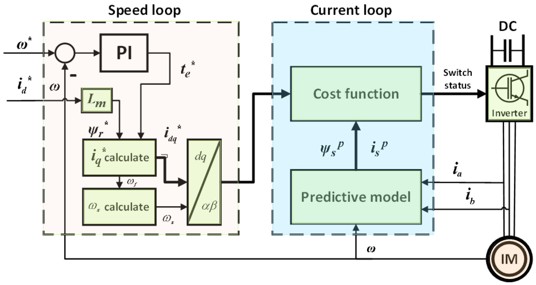
2.2. Traditional Model Predictive Current Control

The structural diagram for MPCC is illustrated in Figure 3. Its outer loop comprises a PI controller, while the inner loop incorporates a discrete predictive model for an induction motor. Voltage vector outputs are selected based on cost functions to track the desired current most effectively.

The forward Euler formula can be represented by Equation (6):

$$\frac{dx}{dt}\approx \frac{x(k+1)-x(k)}{T_s}$$

(6)

In Equation (6), T_s represents the control period. Applying the forward Euler method for discretization, Equations (7) and (8) yield the stator flux prediction equation at time k + 1 and the stator current prediction equation, respectively:

$${\psi }_s^p(k+1)={\psi }_s(k)+T_s[V_s(k)-R_s{i}_s(k)]$$

(7)

$$i_s^p(k+1)=(1+\frac{T_s}{{\tau }_{\sigma }})i_s(k)+\frac{T_s}{{\tau }_{\sigma }+T_s}\{\frac{1}{R_{\sigma }}[\left(\frac{k_r}{{\tau }_r}-k_{r}j\Omega \right){\psi }_r(r)+V_s(k+1)]\}$$

(8)

where ${\tau }_{\sigma }=\frac{\sigma L_s}{R_{\sigma }}$, $R_{\sigma }=R_s+k_r^2{R}_r$, $k_r=\frac{L_m}{L_r}$, ${\tau }_r=\frac{L_r}{R_r}$, ${\tau }_r=\frac{L_r}{R_r}$, and vs. (k + 1) represents the three-phase voltage values of an NPC three-phase inverter output, which are dependent on the inverter’s switching state. Based on the current sampled values i_s (k) at the current time instant, the electrical angular velocity Ω, and all 27 possible output voltage vectors of the inverter at time k + 1, 27 potential stator current prediction values for the next time instant can be derived.

After obtaining the predicted value of the stator current at time k + 1, it is necessary to establish a model to predict the cost function of current control as (9):

$$\left\{\begin{array}{l}\min g=\left|i_{s\alpha i}^p(k+1)-i_{s\alpha }^{*}(k+1)\right|+\left|i_{s\beta i}^p(k+1)-i_{s\beta }^{*}(k+1)\right|\\ s.t. u_s(k)\in \left\{u_0,u_1,\cdots ,u_{27}\right\}\end{array}\right.$$

(9)

The cost function contains only one tracking term for current, allowing for the direct determination of the deviation between the predicted current and the specified current.

2.3. Traditional Design Methods for Switching Frequency Weighting Coefficients

While ensuring a certain level of control performance, minimizing the switching frequency of the inverter can reduce the losses of power semiconductor devices. This can be achieved by constraining the number of switches in the inverter. As such, n is defined as the number of switching transitions of the inverter’s switch state from S(k − 1) to S(k), as shown in Equation (10):

$$n={\displaystyle \sum \left|S_x(k)-S_x(k-1)\right|}\hspace{1em}\hspace{1em}\hspace{1em}\hspace{1em}\hspace{1em}(x=a,b,c)$$

(10)

From Figure 1, it is evident that the switching states of each bridge leg in the three-phase inverter can be represented as S = (S_a, S_b, S_c). Based on Equation (10), the cost function with the constraint on switching frequency can be obtained:

$$\left\{\begin{array}{l}\min g_n=\left|i_{s\alpha i}^p(k+1)-i_{s\alpha }^{*}(k+1)\right|+\left|i_{s\beta i}^p(k+1)-i_{s\beta }^{*}(k+1)\right|+{\lambda }_n\cdot n\\ s.t. u_s(k)\in \left\{u_0,u_1,\cdots ,u_{27}\right\}\end{array}\right.$$

(11)

where λ_n represents the weighting coefficient of the switching frequency term in the cost function (11).

When considering the inverter’s switching frequency, a model predictive control scheme is typically designed to optimize the switching losses. However, the dimensions of the penalty terms for current and switching frequency in the cost function are different, making it challenging to design appropriate weighting coefficients. Currently, there is limited theoretical analysis of the weighting coefficients for switching frequency in research. Therefore, the following section elaborates on the design approach for the weighting coefficients of the switching frequency, providing a theoretical basis for optimizing switching losses.

3. Proposed Improved Cost Function Design Method

3.1. Proposed Method for Weighting Coefficient Design with Unified Dimensions

Based on the current prediction from Equation (8), the relationship between the voltage vector and the predicted current vector can be derived:

$$V_s(k+1)=\frac{{\tau }_{\sigma }+T}{T_s}{i}_s^p(k+1)-\frac{{\tau }_{\sigma }+T}{T_s}(1+\frac{T_s}{{\tau }_{\sigma }})i_s(k)+\frac{1}{R_{\sigma }}\left(\frac{k_r}{{\tau }_r}-k_{r}j\Omega \right){\psi }_r(r)$$

(12)

Subsequently, based on (3) and (12), the relationship between the inverter switching states and the predicted currents can be established as Equation (13):

$$\frac{V_{dc}}{3}(S_a+a{S}_b+a^2{S}_c)=\frac{{\tau }_{\sigma }+T}{T_s}{\mathit{i}}_s^p(k+1)-\frac{{\tau }_{\sigma }+T}{T_s}(1+\frac{T_s}{{\tau }_{\sigma }}){\mathit{i}}_s(k)+\frac{1}{R_{\sigma }}\left(\frac{k_r}{{\tau }_r}-k_{r}j\Omega \right){\mathsf{\psi }}_r(r)$$

(13)

Due to the high sampling frequency of the MPCC strategy, within the same sampling interval, it is assumed that i_s (k) and Ψ_r (k) are constant. The relationship between the inverter switching count and the predicted currents can thus be expressed by Equation (14):

$$(\Delta S_a+a\Delta S_b+a^2\Delta S_c)=\frac{3}{V_{dc}}\frac{{\tau }_{\sigma }+T}{T_s}(i_{s\mathrm{j}}^p(k+1)-i_{si}^p(k+1))$$

(14)

where

$$i_{si}^p(k+1)\in \left\{i_{s0}^p(k+1),i_{s1}^p(k+1),\cdots ,i_{s27}^p(k+1)\right\}$$

and $i_{s\mathrm{j}}^p(k+1)$ represents the optimal vector chosen at the preceding time instant.

Then, applying the inverse Clarke transformation to Equation (14) derives (15):

$$\left[\begin{array}{c}\Delta S_a\\ \Delta S_b\\ \Delta S_c\end{array}\right]=\frac{3}{V_{dc}}\frac{{\tau }_{\sigma }+T}{T_s}\left[\begin{array}{c}\Delta {\mathit{i}}_{sa}^p(k+1)\\ \Delta {\mathit{i}}_{sb}^p(k+1)\\ \Delta {\mathit{i}}_{sc}^p(k+1)\end{array}\right]$$

(15)

Based on Equations (10) and (15), the expression for the switching frequency of three-phase inverters can be obtained:

$$n=\frac{3}{V_{dc}}\frac{{\tau }_{\sigma }+T}{T_s}(\left|\Delta {\mathrm{i}}_{sa}^p(k+1)\right|+\left|\Delta {\mathrm{i}}_{sb}^p(k+1)\right|+\left|\Delta {\mathrm{i}}_{sc}^p(k+1)\right|)$$

(16)

Therefore, the expression for the weighting coefficient λ_n of the constrained switching frequency term is given by Equation (17):

$${\lambda }_n=\frac{T_s}{{\tau }_{\sigma }+T_s}\frac{V_{dc}}{3}$$

(17)

then, we define ξ as the new weighting coefficient:

$$\xi ={\lambda }_n\cdot n$$

(18)

Finally, the cost function with weighting coefficient dimension unification, accounting for the switching frequency term, is expressed as Equation (19):

$$\left\{\begin{array}{l}\min g=(1-\epsilon )(\left|i_{s\alpha i}^p(k+1)-i_{s\alpha }^{*}(k+1)\right|+\left|i_{s\beta i}^p(k+1)-i_{s\beta }^{*}(k+1)\right|)+\epsilon \cdot \xi \\ s.t. u_s(k)\in \left\{u_0,u_1,\cdots ,u_{27}\right\},\epsilon \in [0,1]\end{array}\right.$$

(19)

Here, ε is a newly introduced weighting coefficient variable used to adjust the balance between the current tracking and the switching frequency constraints in the objective function. When ε is set to 0, it indicates no limitation on the switching frequency. As ε increases, the contribution of the switching frequency constraint in the objective function gradually rises.

Accordingly, ε can be designed based on requirements such as current harmonic content, maximum switching frequency allowable by the inverter power semiconductor devices, and system heat dissipation. While ε still needs to be carefully chosen, Equation (17) provides a better representation of the proportion between current and switching frequency compared to the traditional objective function (11), as both terms are now dimensionally unified. In practical controller implementations, due to truncation errors inherent in DSPs, FPGAs, and similar chips, Equation (17) expands the range of deployable chips for this algorithm and reduces the risk of vector selection errors that may arise from truncation errors.

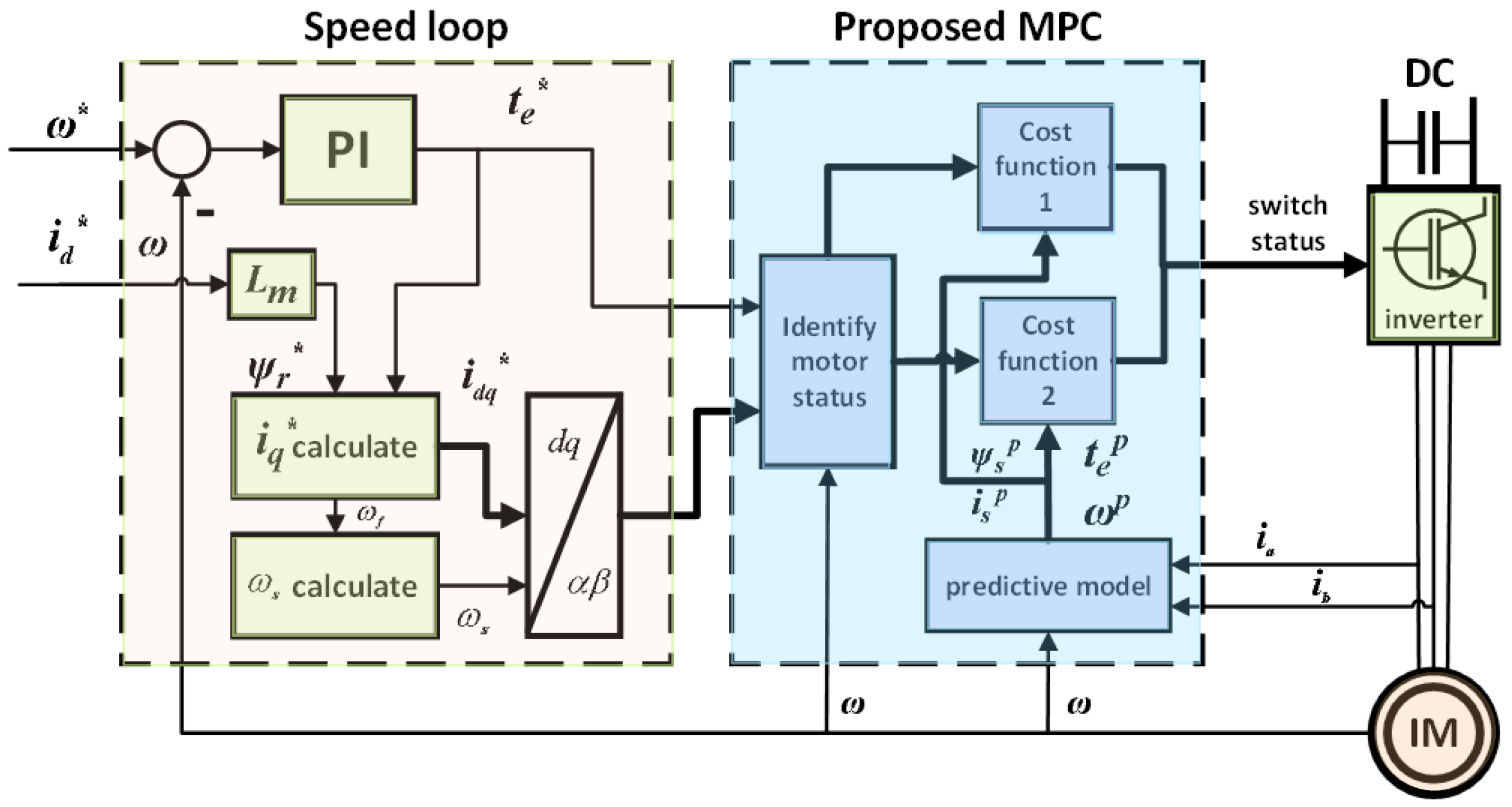
3.2. Proposed Composite Cost Function for Model Predictive Control

As the motor requires excellent torque and speed tracking performance during the startup phase, and emphasizes current tracking performance more in steady-state operation, the control proposed in this paper for the MPC algorithm with composite cost functions meets these requirements. The structural diagram is depicted in Figure 4, and the expression for the composite cost function is given by Equation (20):

$$\begin{array}{l}g=\left\{\begin{array}{c}{g}_1,△\omega <n\%\times {\omega }^{*}\\ g_2,△\omega \ge n\%\times {\omega }^{*}\end{array}\right.\\ g_1=(1-\epsilon )(\left|i_{s\alpha i}^p(k+1)-i_{s\alpha }^{*}(k+1)\right|+\left|i_{s\beta i}^p(k+1)-i_{s\beta }^{*}(k+1)\right|)+\epsilon \cdot \xi \\ g_2={\lambda }_{\omega }\times {\left|{\omega }^p(k+1)-{\omega }^{*}\right|}^2 +{\lambda }_{\psi }\times {\left|\left|{\psi }_s^p(k+1)\right|-\left|{\psi }_s^{*}\right|\right|}^2+h_n\end{array}$$

(20)

where ∆ω represents the speed deviation, ω* denotes the desired speed, ω stands for the actual speed, λ_ω, and λ_Ψ are weighting coefficients, h_n represents the penalty term for torque overshoot, and n represents the index of the switch state.

From the aforementioned expression of the cost function, it is evident that during the dynamic phase of the motor, the optimization focuses on speed and flux as key factors (using g₂). However, during steady-state operation, the emphasis shifts to tracking current and appropriately limiting switch frequency (using g₁). In particular, in g₂, λ_ω and λ_Ψ represent the reciprocal of the maximum speed and stator flux, respectively. This means that λ_ω and λ_Ψ have adjusted the speed limit term and stator flux limit term to between 0–1, unifying their magnitudes. h_n represents the penalty term for torque overshoot. If the predicted torque exceeds the torque limit value, h_n = ∞, this means that the vector is not selected.

To quantify the switching frequency of inverters, we define the average number of switching actions, denoted as n_ek, for all power switching devices in a three-phase inverter within one control cycle.

$$n_{ek}={\displaystyle \sum _{i=1}^4\frac{n_{ai}+n_{bi}+n_{ci}}{12}}$$

(21)

where k denotes the control cycle sequence and n_ai {i∈[1–4]} represents the number of switching actions for the power switching device in phase-a during the first control cycle.

Then, the average switching frequency of the inverter is defined as f_e:

$$f_e=\frac{{\displaystyle \sum _{k=1}^N{n}_{ek}}}{N\times T_s}$$

(22)

where N represents the total number of control cycles simulated up to the current instant and T_s denotes the control cycle step size.

In consideration of the characteristic of variable switching frequency in MPCC, which does not possess a fixed switching frequency, it is inadequate to evaluate the switching frequency merely based on the average value. To comprehensively assess the inverter’s switching frequency, we hereby define the instantaneous switching frequency f_s, as follows:

$$f_s=\frac{{\displaystyle \sum _{k=1}^{N_1}{n}_{ek}}}{T_{s1}}$$

(23)

where T_s1 denotes a fixed small period and N₁ represents the number of control cycles contained within T_s1.

The instantaneous switching frequency indicates the average number of power switch device actions within a small period. Since T_s1 is significantly smaller than the entire simulation period, we approximate the instantaneous switching frequency as f_s.

4. Simulation and Experimental

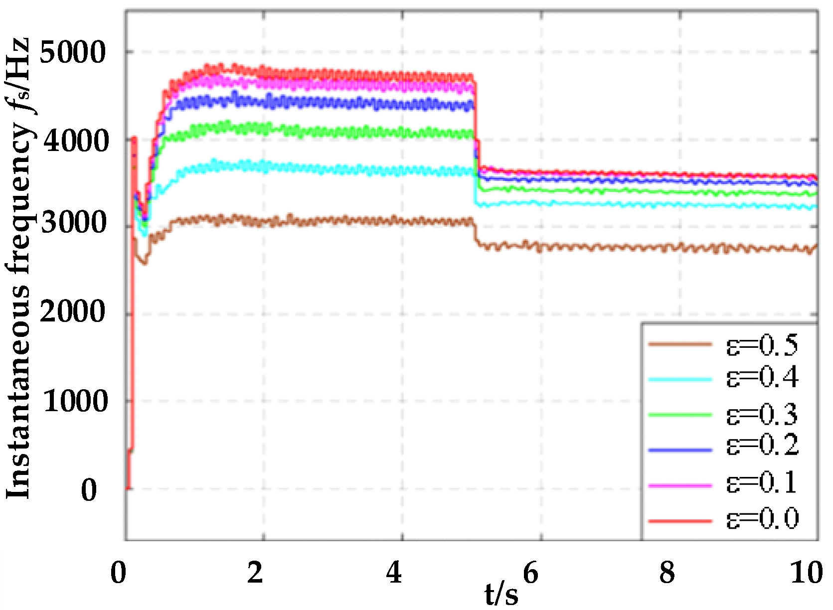
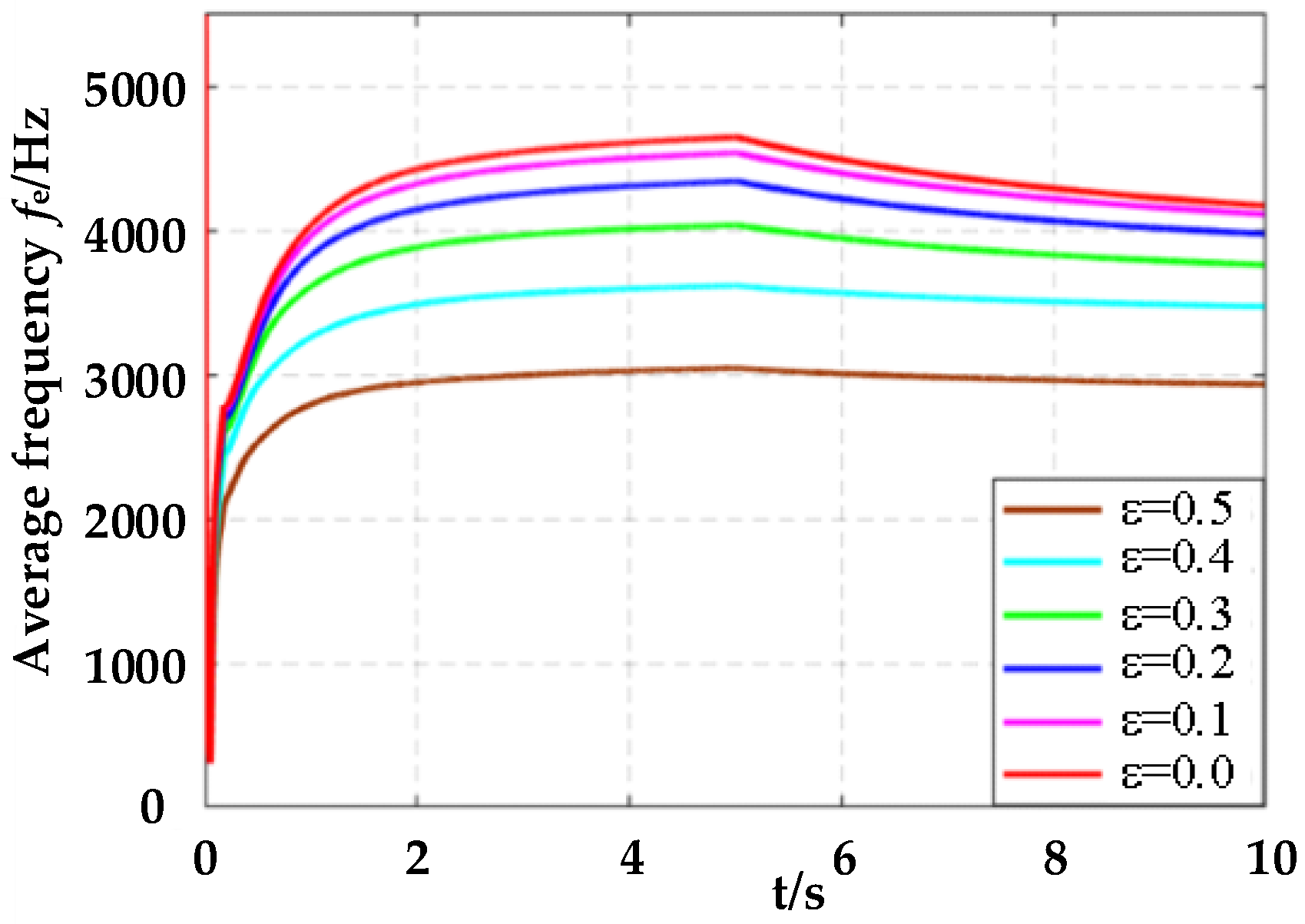
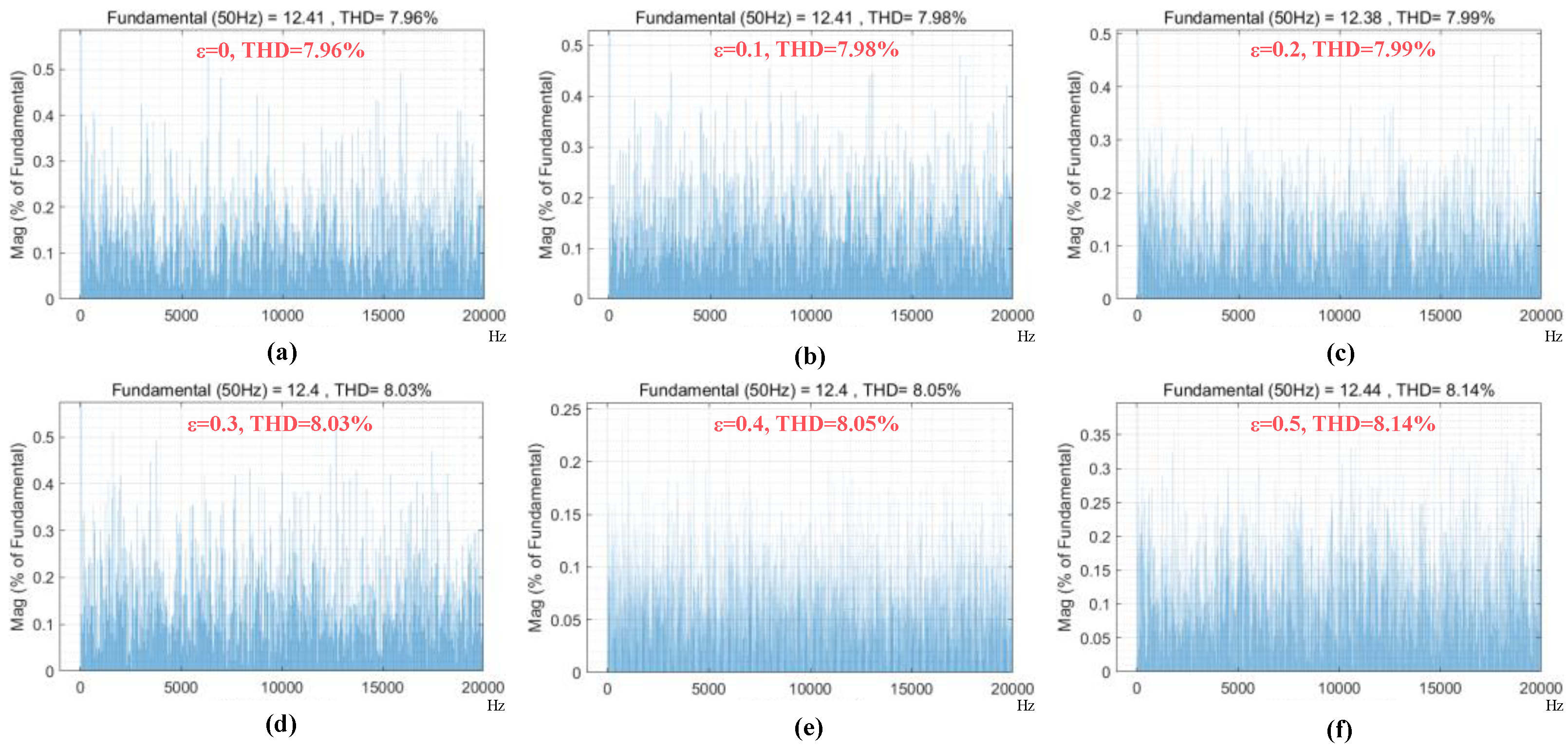
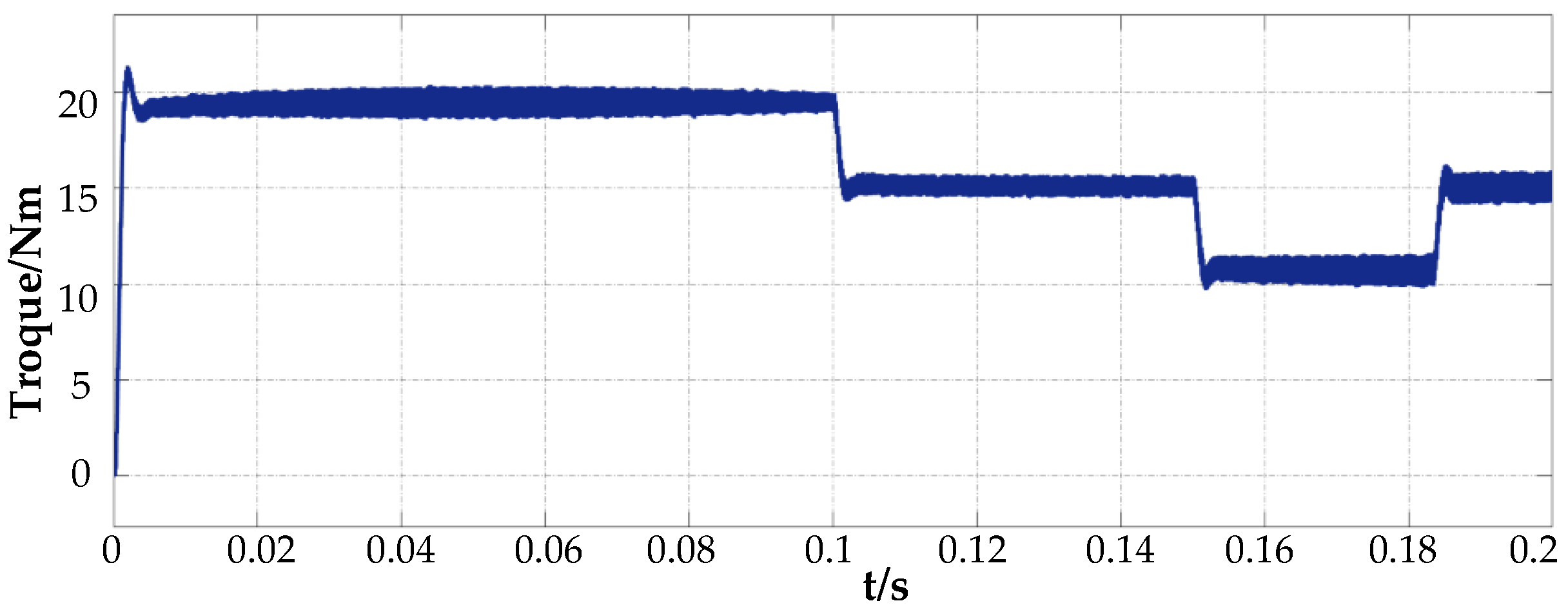
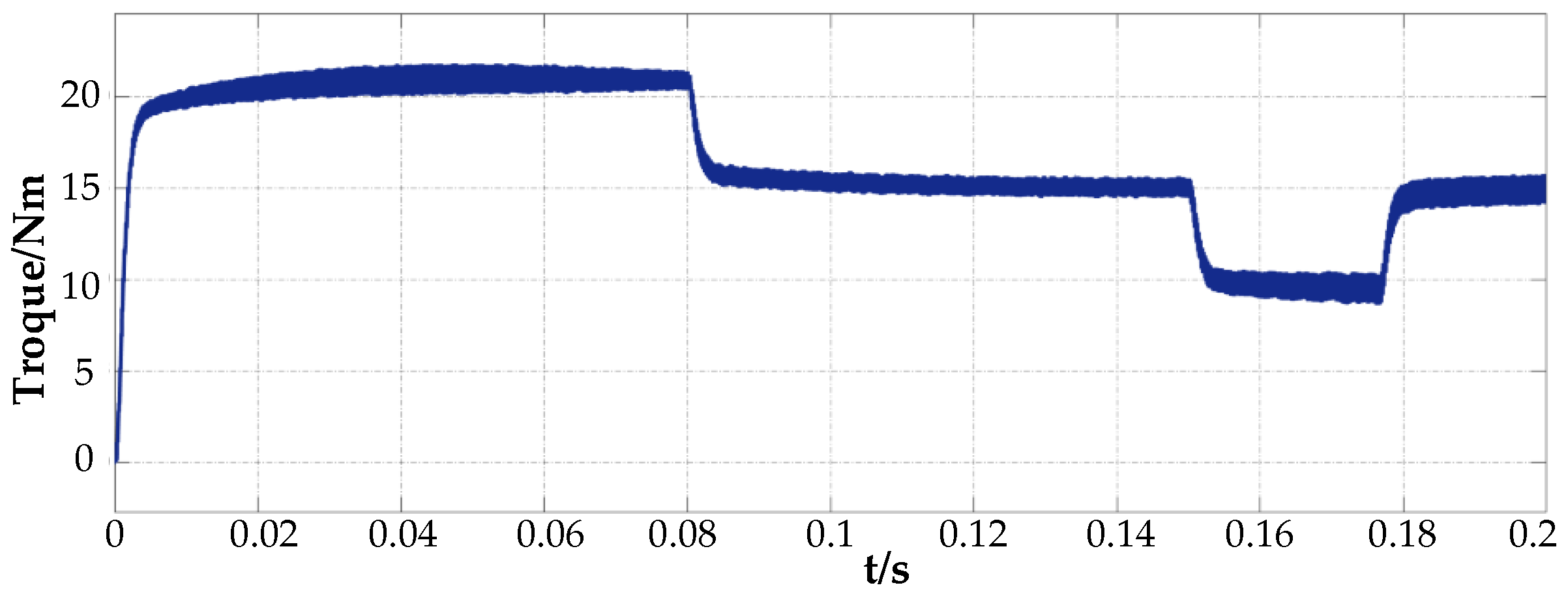
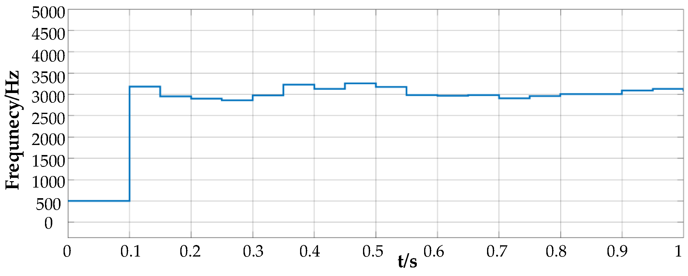
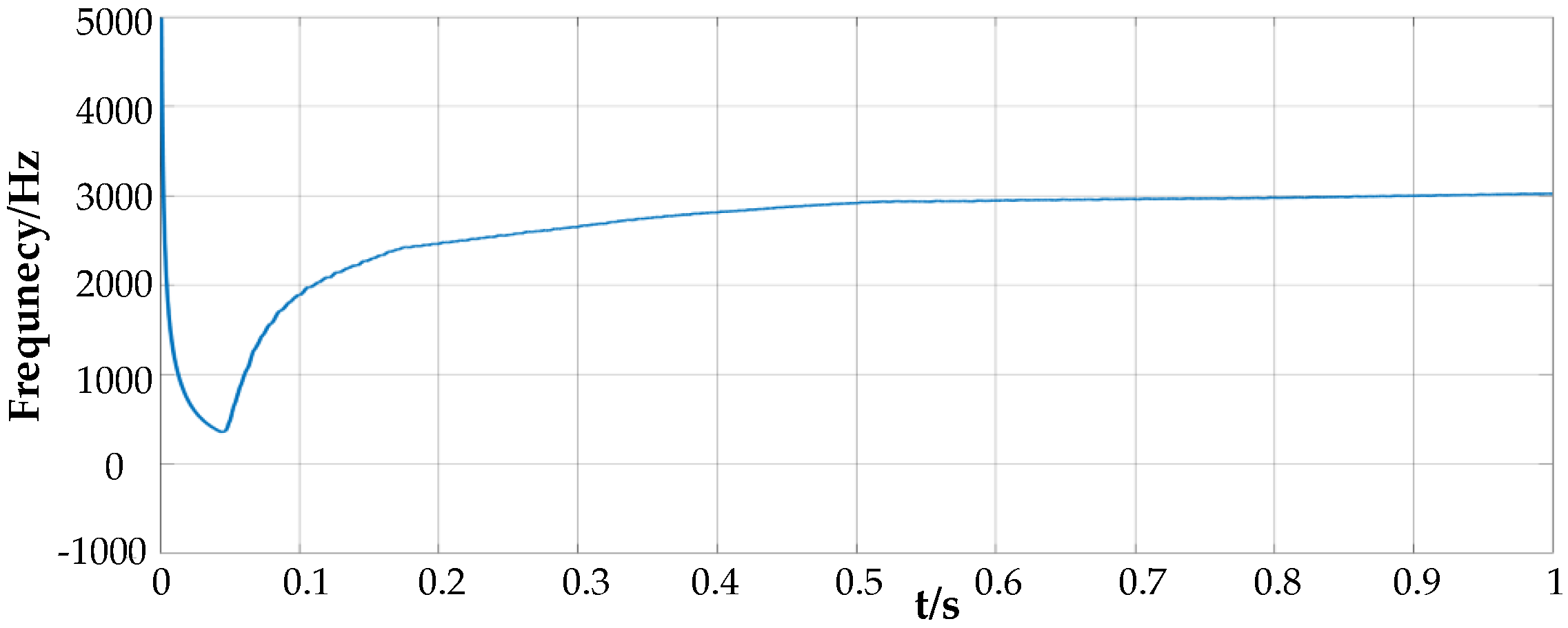
4.1. Simulation Verification of the Proposed Method

This section presents a simulation of induction motors (IM) undergoing a 10 Nm load startup, and motor parameters in Matlab/Simulink (R2022b) are presented in

Table 1. Motor parameters.

Parameter	Value	Unit
Sampling period	25	μs
DC-Link voltage	500	Vdc/V
DC capacitor	900	μF
Rated Speed	1500	rpm
Stator resistance	1	Rs/Ω
Rotor resistance	0.98	Rr/Ω
Stator inductance	0.00223	Ls/H
Rotor inductance	0.00224	Lr/H
Mutual inductance	0.002	Lm/H
Pole pairs	2	-

. During simulations and experiments, a composite cost function is used, where g₂ is used during the motor start-up phase and g₁ is used during the motor steady-state phase. The following is an analysis of the simulation results.

Figure 5 illustrates the simulation waveform of the instantaneous switching frequency, f_s, of the inverter, and Figure 6 depicts the simulation waveform of the average switching frequency, f_e, of the inverter. During the simulation, the motor accelerates from 0 rpm to 1500 rpm and then decelerates to 1000 rpm after 5 s. The values of ε are set to 0.0, 0.1, 0.2, 0.3, 0.4, and 0.5, corresponding to various weighting coefficients.

From Figure 5 and Figure 6, it can be observed that with the continuous increase of ε, which corresponds to the increasing proportion of the constraint on the switching frequency term in the objective function, both the maximum f_s and the f_e of the inverter decrease accordingly. The simulation results indicate that after adopting the proposed scheme of adjusting the weighting coefficients for the constraint on the switching frequency term, only the proportion of the switching frequency term in the objective function needs to be adjusted, i.e., changing the value of ε. A larger ε leads to a greater proportion of the constraint on the switching frequency term in the objective function.

In Figure 6, when ε = 0.5, as the induction motor accelerates to 1500 rpm, its f_s stabilizes around 3 kHz. When the motor decelerates to 1000 rpm, the f_s begins to decrease gradually and eventually stabilizes around 2.8 kHz. Throughout the entire speed regulation range of the induction motor, the inverter may operate steadily at different speeds. This control algorithm, which varies the switching frequency according to the motor speed, results in different switching frequencies of the inverter.

Figure 7 presents the FFT analysis results of phase-a current with different weight coefficients ε (motor operating condition is 1500 rpm in the steady-state stage). As shown in Figure 7a, when ε = 0, it means that the g₁ cost function used in the steady-state stage of the motor only constrains the stator current and does not limit the switching frequency. At this condition, the phase-a current THD is 7.96%. As ε gradually increases, it means that the switching frequency limitation term in g₁ begins to take effect. In this case, the switching frequency gradually decreases (Figure 5 and Figure 6), but the current harmonics of phase-a gradually increase (Figure 7b–f). The THD at ε = 0.5 is -increased by approximately 2.3% compared to ε = 0.

Figure 8 shows the total loss (including switching losses and conduction losses) of all IGBTs and Diodes in phase-a at different ε. The simulation is based on PLECS tools in Matlab/Simulink, and simulation data is based on Infineon FS3L50R07W2H3_B11. As illustrated in Figure 8, as ε increases from 0 to 0.5, the total loss decreases from 11.252 W to 10.6047 W, with a decrease of 5.75%.

Table 2. Simulation results of different operating points.

Speed	ε = 0			ε = 0.1			ε = 0.2			ε = 0.3			ε = 0.4			ε = 0.5
	THD	fs	Loss	THD	fs	Loss	THD	fs	Loss	THD	fs	Loss	THD	fs	Loss	THD	fs	Loss
Low Speed (300 rpm)	7.93%	1.4	9.298	7.94%	1.35	9.199	7.97%	1.31	9.105	8.00%	1.24	9.113	8.05%	1.19	8.909	8.07%	1.15	8.589
Medium Speed (900 rpm)	7.94%	3.8	10.311	7.94%	3.75	10.254	7.98%	3.7	10.102	7.97%	3.5	10.032	8.01%	3.4	9.899	8.10%	2.8	9.582
High Speed (1500 rpm)	7.96%	4.8	11.252	7.98%	4.7	11.241	7.99%	4.5	11.096	8.03%	4.1	11.048	8.05%	3.7	10.964	8.14%	3.0	10.605

: f_s ≤ 2 kHz; : 2 kHz < f_s ≤ 4 kHz; : f_s > 4 kHz.

presents the simulation results at different operating points: low speed (300 rpm), medium speed (900 rpm), and high speed (1500 rpm). According to the data in Table 2, when the motor speed is low, the switching frequency is also low. As the speed increases, the switching frequency also increases. A detailed analysis reveals that as the motor speed decreases, indicating a lower fundamental frequency of the motor phase current, the MPC algorithm requires less frequent switching of vectors to achieve current tracking, and the switching frequency consequently decreases. As the speed increases, the fundamental frequency of the motor phase current also rises, necessitating more frequent vector switching by the MPC algorithm to accomplish current tracking, thereby resulting in an increase in the switching frequency. In practical engineering applications, ε can be dynamically selected according to the operating conditions of the motor. Under low-speed motor conditions, if the switching frequency is within an acceptable range, reducing ε appropriately can improve the quality of the current waveform. However, in high-speed motor conditions, sacrificing some quality of the current waveform may be necessary to ensure that the switching frequency does not exceed the specified limit (increasing ε), thereby maintaining the inverter within a safe operating region.

The above simulation results demonstrate the effectiveness of the unified dimensional cost function proposed in this article in limiting switching frequency (g₁). In practical applications, the appropriate ε should be selected according to the needs. The selection of the appropriate ε can reduce switching frequency while minimizing the increase of THD, thereby reducing inverter losses and improving the service life of motor drive systems.

Comparing Figure 9 and Figure 10, it is evident that speed has a rapid response during the motor startup phase when employing a composite cost function in (20). As the motor accelerates from 0 rpm to 1500 rpm, the MPC of composite cost function achieves an acceleration time of approximately 0.08 s, whereas the MPC with the classical cost function predicts an acceleration time of about 0.1 s, resulting in a 20% improvement in speed response.

Comparing Figure 11 and Figure 12, we can see that simulation results demonstrate the effectiveness of the composite cost function in enhancing the torque response performance of MPC during the motor startup phase.

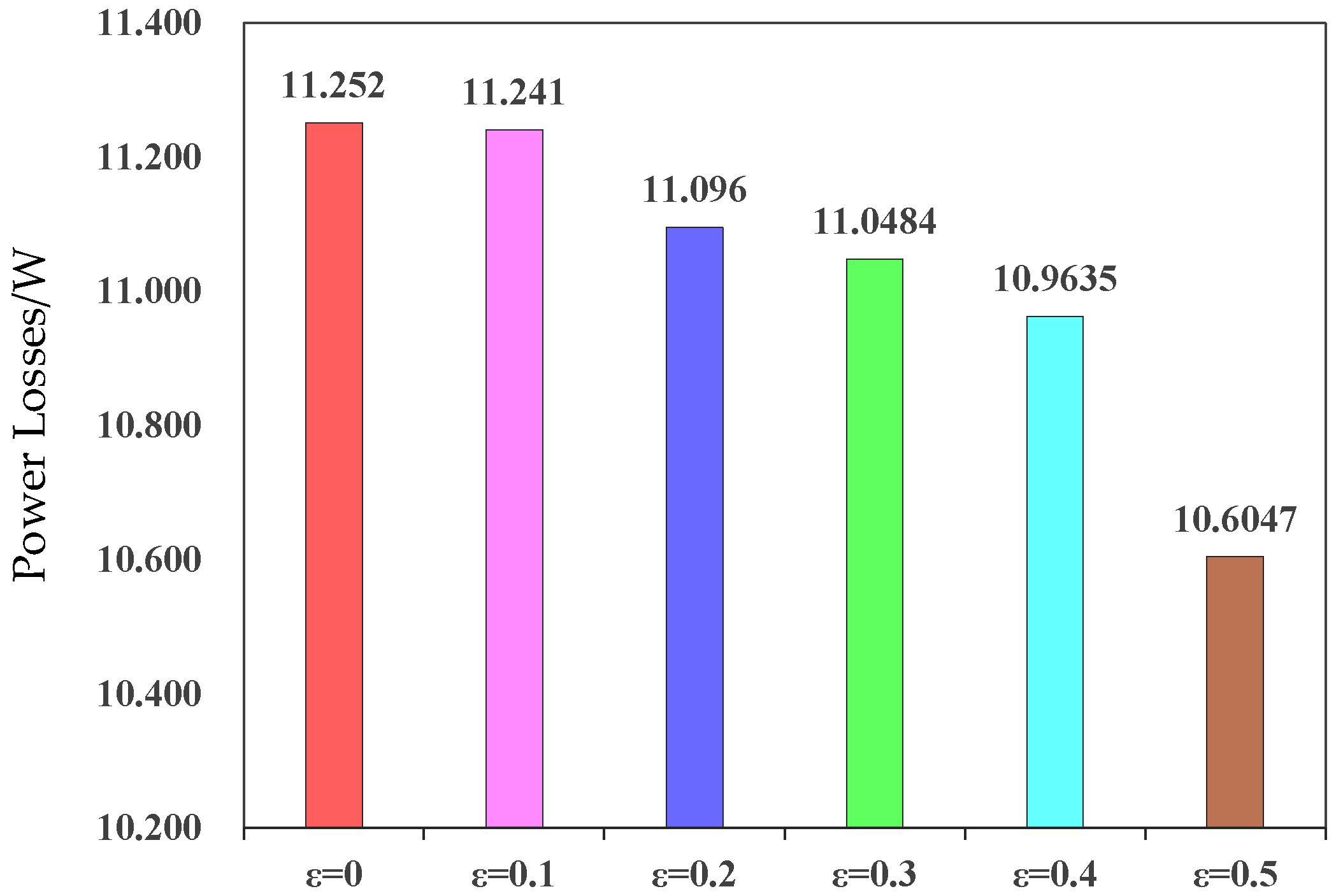
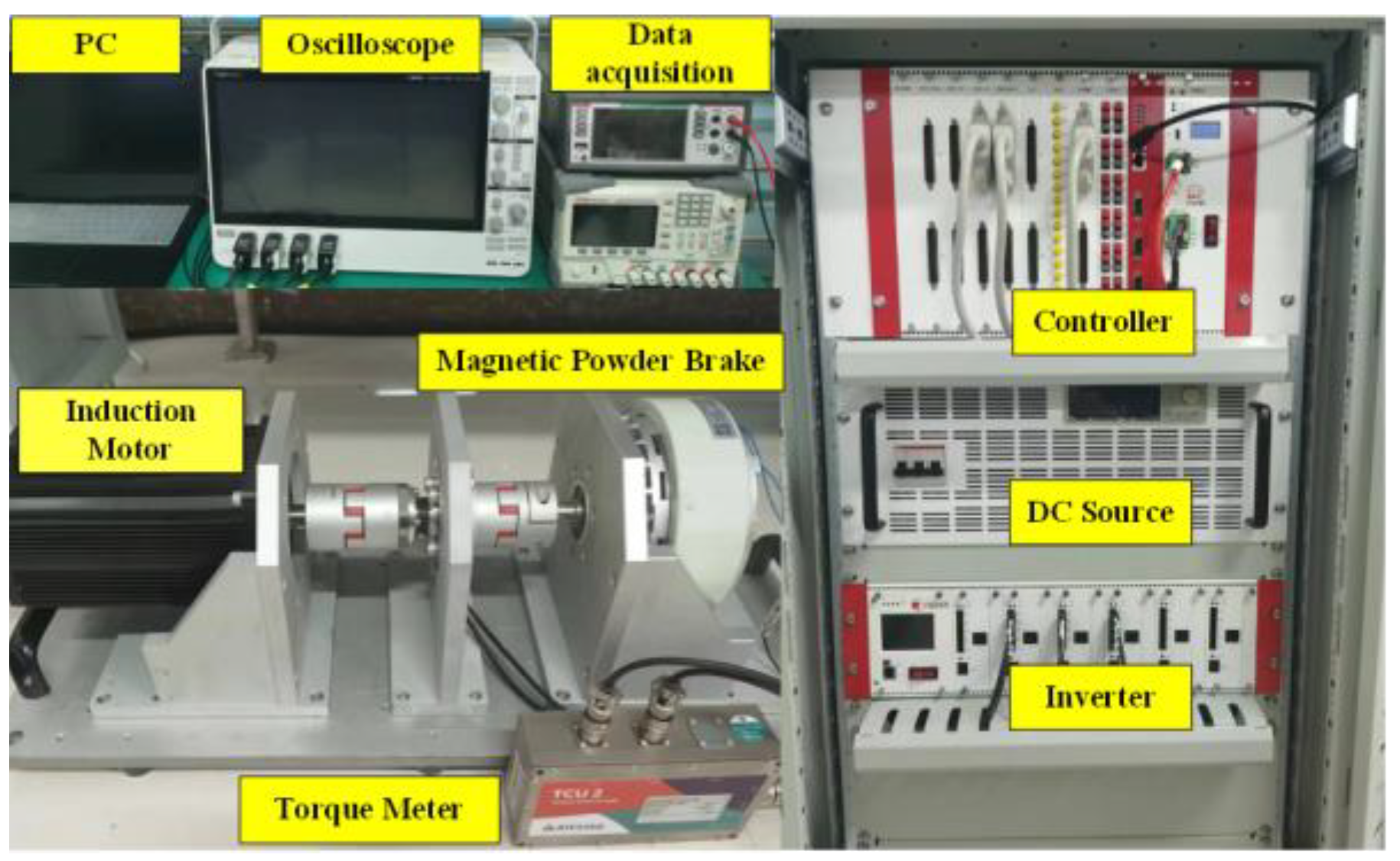
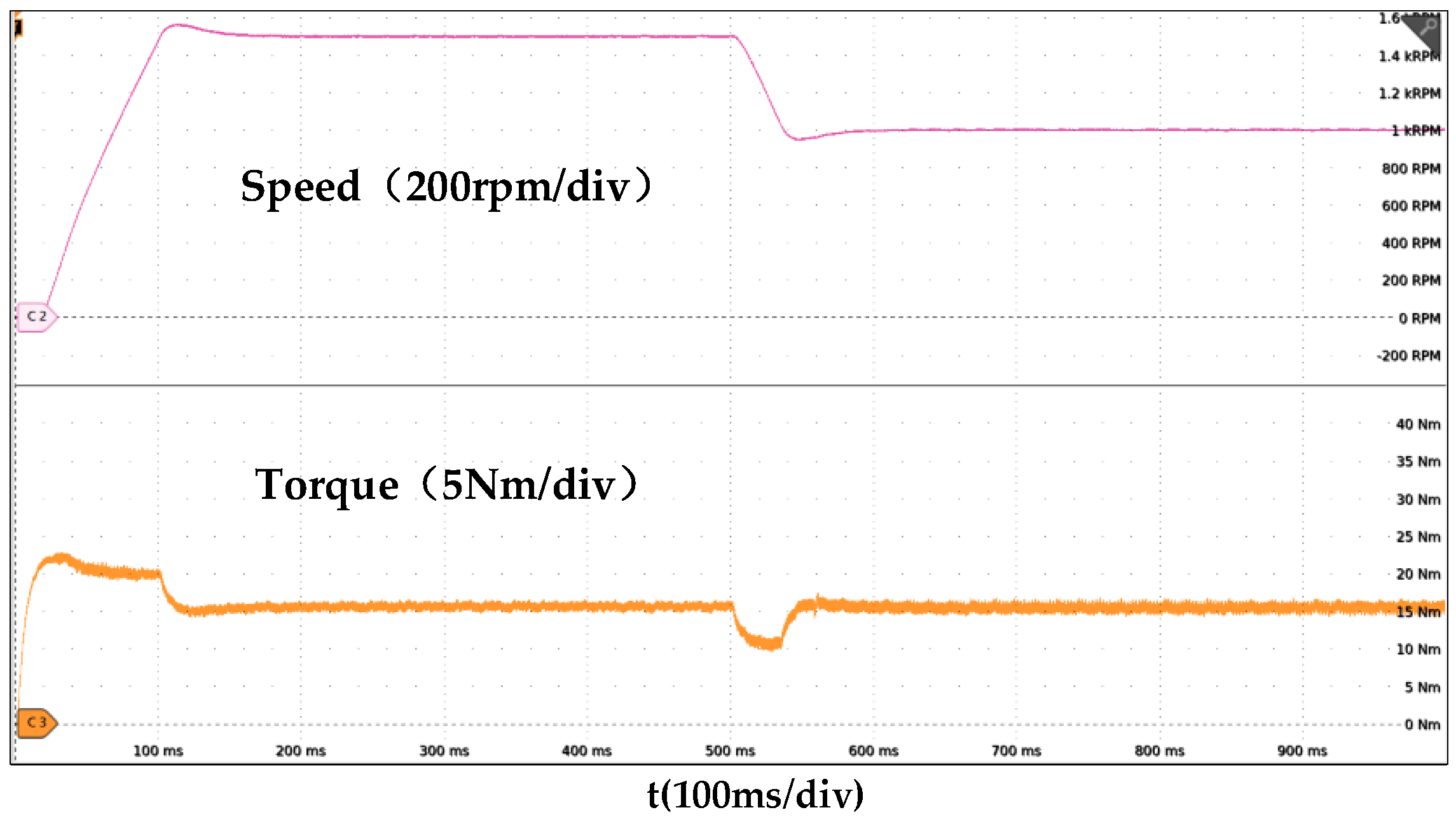
4.2. Experimental Results and Analysis

The experimental platform of a 15 Nm load startup for IM is illustrated in Figure 13. During the experiments, the chip used is a TMS320F28377 (Texas Instruments, Dallas, TX, USA), employing a composite cost function to control the speed regulation system of an induction motor driven by a three-level inverter. The instantaneous and average switching frequencies of the inverter can be calculated by measuring the PWM pulses emitted by the DSP controller. The following is an analysis of the experimental results.

Figure 14 and Figure 15 present a comparison of torque measurement waveforms for the motor utilizing the proposed composite cost function and traditional cost function within the MPC framework. The utilization of the composite cost function model demonstrates a certain effectiveness in achieving rapid tracking of the desired torque during the motor start-up phase under current control. From Figure 14 and Figure 15, we can see that the experimental waveforms of speed and torque are consistent with the simulation results.

Then, the induction motor is set to accelerate from 0 rpm to 1500 rpm, with the weighting coefficient ε = 0.5 introduced for the switching frequency constraint term in the model predictive control cost function. The instantaneous switching frequency of the induction motor during this acceleration process is depicted in Figure 16 and the average switching frequency is shown in Figure 17.

As depicted in Figure 16, the instantaneous switching frequency throughout the experimental steady-state process is limited to 3000 Hz, and Figure 17 shows that the average switching frequency is about 3000 Hz. We can see that the experimental waveforms of switching frequency demonstrate the correctness of the weighting coefficient design.

5. Conclusions

This paper presents a method for designing the weighting coefficients in the MPC cost function, which unifies the dimensions of the penalty terms for stator current and switching frequency. The unified dimensional expression for both provides a theoretical basis for selecting the weighting coefficients for the switching frequency term. These coefficients can be designed considering factors such as the maximum switching frequency tolerable by the inverter power switches and system heat dissipation requirements, aiming to appropriately reduce the switching frequency. Furthermore, to address the slow speed and torque response issue of MPC during motor start-up, a composite cost function MPC control strategy is proposed, enhancing dynamic response performance. Through simulation and experimental validation, the proposed method is employed to design the cost function using the weighting coefficient selection approach, and various motor operating conditions are tested. Analysis of the results demonstrates the effectiveness of the proposed approach in reducing switching frequency and achieving satisfactory performance across the entire speed range.

References

1. Zhang, X.; Ma, Z.; Niu, H.; Huang, J.; Lin, G. Finite-Control-Set Model-Predictive Control with Data-Driven Switching Frequency Control for Single-Phase Three-Level NPC Rectifiers. IEEE Trans. Ind. Electron. 2024, 71, 7180–7189. [Google Scholar] [CrossRef]
2. De Martin, I.D.; Brosch, A.; Tinazzi, F.; Zigliotto, M. Continuous Control Set Model Predictive Torque Control with Minimum Current Magnitude Criterion for Synchronous Motor Drives. IEEE Trans. Ind. Electron. 2023, 71, 6787–6796. [Google Scholar] [CrossRef]
3. Zhao, B.; Li, H.; Mao, J. Double-Objective Finite Control Set Model-Free Predictive Control with DSVM for PMSM Drives. J. Power Electron. 2019, 19, 168–178. [Google Scholar]
4. Yang, Q.; Karamanakos, P.; Liegmann, E.; Tian, W.; Geyer, T.; Kennel, R.; Heldwein, M.L. A Fixed Switching Frequency Direct Model Predictive Control for Neutral-Point-Clamped Three-Level Inverters with Induction Machines. IEEE Trans. Power Electron. 2023, 38, 13703–13716. [Google Scholar] [CrossRef]
5. Sun, Z.; Xu, S.; Ren, G.; Yao, C.; Ma, G.; Jatskevich, J. Weighting-Factor-Less Model Predictive Control with Multiobjectives for Three-Level Hybrid ANPC Inverter Drives. IEEE J. Emerg. Sel. Top. Power Electron. 2023, 11, 4726–4738. [Google Scholar] [CrossRef]
6. Bao, G.; Qi, W.; He, T. Direct Torque Control of PMSM with Modified Finite Set Model Predictive Control. Energies 2020, 13, 234. [Google Scholar] [CrossRef]
7. Wang, F.; Zhang, Z.; Mei, X.; Rodriguez, J.; Kennel, R. Advanced Control Strategies of Induction Machine: Field Oriented Control, Direct Torque Control and Model Predictive Control. Energies 2018, 11, 120. [Google Scholar] [CrossRef]
8. Feng, S.; Wei, C.; Lei, J. Reduction of Prediction Errors for the Matrix Converter with an Improved Model Predictive Control. Energies 2019, 12, 3029. [Google Scholar] [CrossRef]
9. Bakini, H.; Mesbahi, N.; Kermadi, M.; Mekhilef, S.; Zahraoui, Y.; Mubin, M.; Seyedmahmoudian, M.; Stojcevski, A. An Improved Mutated Predictive Control for Two-Level Voltage Source Inverter with Reduced Switching Losses. IEEE Access 2024, 12, 25797–25808. [Google Scholar] [CrossRef]
10. Li, T.; Sun, X.; Lei, G.; Guo, Y.; Yang, Z.; Zhu, J. Finite-Control-Set Model Predictive Control of Permanent Magnet Synchronous Motor Drive Systems—An Overview. IEEE/CAA J. Autom. Sin. 2022, 9, 2087–2105. [Google Scholar] [CrossRef]
11. Wang, W.; Lu, Z.; Hua, W.; Wang, Z.; Cheng, M. Simplified Model Predictive Current Control of Primary Permanent-Magnet Linear Motor Traction Systems for Subway Applications. Energies 2019, 12, 4144. [Google Scholar] [CrossRef]
12. Arahal, M.R.; Barrero, F.; Satué, M.G.; Ramírez, D.R. Predictive Control of Multi-Phase Motor for Constant Torque Applications. Machines 2022, 10, 211. [Google Scholar] [CrossRef]
13. Arahal, M.R.; Barrero, F.; Durán, M.J.; Ortega, M.G.; Martín, C. Trade-offs analysis in predictive current control of multi-phase induction machines. Control Eng. Pract. 2018, 81, 105–113. [Google Scholar] [CrossRef]
14. Abbaszadeh, A.; Khaburi, D.A.; Mahmoudi, H.; Rodríguez, J. Simplified Model Predictive Control with Variable Weighting Factor for Current Ripple Reduction. IET Power Electron. 2017, 10, 1165–1174. [Google Scholar] [CrossRef]
15. Kowal G., A.; Arahal, M.R.; Martin, C.; Barrero, F. Constraint Satisfaction in Current Control of a Five-Phase Drive with Locally Tuned Predictive Controllers. Energies 2019, 12, 2715. [Google Scholar] [CrossRef]
16. Arahal, M.R.; Satué, M.G.; Barrero, F.; Ortega, M.G. Adaptive Cost Function FCSMPC for 6-Phase IMs. Energies 2021, 14, 5222. [Google Scholar] [CrossRef]
17. Lin, S.; Fang, X.; Wang, X.; Yang, Z.; Lin, F. Multiobjective Model Predictive Current Control Method of Permanent Magnet Synchronous Traction Motors with Multiple Current Bounds in Railway Application. IEEE Trans. Ind. Electron. 2022, 69, 12348–12357. [Google Scholar] [CrossRef]
18. Davari, S.A.; Nekoukar, V.; Azadi, S.; Flores-Bahamonde, F.; Garcia, C.; Rodriguez, J. Discrete Optimization of Weighting Factor in Model Predictive Control of Induction Motor. IEEE Open J. Ind. Electron. Soc. 2023, 4, 573–582. [Google Scholar] [CrossRef]
19. Kaymanesh, A.; Chandra, A.; Al-Haddad, K. Model Predictive Control of MPUC7-based STATCOM using Autotuned Weighting Factors. IEEE Trans. Ind. Electron. 2022, 69, 2447–2458. [Google Scholar] [CrossRef]
20. Karamanakos, P.; Geyer, T. Guidelines for the design of finite control set model predictive controllers. IEEE Trans. Power Electron. 2020, 35, 7434–7450. [Google Scholar] [CrossRef]
Figure 1. Topology of NPC inverter with IM.
Energies 17 02479 g001
Figure 2. All possible switching states and voltage vectors in three-level inverters.
Energies 17 02479 g002
Figure 3. Traditional MPCC control structure diagram.
Energies 17 02479 g003
Figure 4. Schematic diagram of MPC structure for composite cost functions.
Energies 17 02479 g004
Figure 5. The instantaneous switching frequency of the inverter.
Energies 17 02479 g005
Figure 6. The average switching frequency of the inverter.
Energies 17 02479 g006
Figure 7. The phase-a current THD values at different ε. (a) ε = 0. (b) ε = 0.1. (c) ε = 0.2. (d) ε = 0.3. (e) ε = 0.4. (f) ε = 0.5.
Energies 17 02479 g007
Figure 8. The total power loss values at different ε.
Energies 17 02479 g008
Figure 9. The speed simulation waveform of traditional MPC (only using g1).
Energies 17 02479 g009
Figure 10. The speed simulation waveform of MPC based on the composite cost function.
Energies 17 02479 g010
Figure 11. The torque simulation waveform of traditional MPC (only using g1).
Energies 17 02479 g011
Figure 12. The torque simulation waveform of MPC based on the composite cost function.
Energies 17 02479 g012
Figure 13. The experimental platform.
Energies 17 02479 g013
Figure 14. The experimental waveforms of traditional MPC (only using g1).
Energies 17 02479 g014
Figure 15. The experimental waveforms of MPC based on the composite cost function.
Energies 17 02479 g015
Figure 16. The instantaneous switching frequency of the inverter when ε = 0.5.
Energies 17 02479 g016
Figure 17. The average switching frequency of the inverter when ε = 0.5.
Energies 17 02479 g017