Abstract
Based on Thermodynamics and its well-established First and Second Laws, this work presents and explores their economics counterparts, introducing new concepts, variables, and equations. This includes, among others, the economic counterparts of temperature, reversibility and irreversibility, and entropy and entropy generation resulting from economic irreversibility. The meaning of the new concepts, variables, equations, and their messages are introduced and discussed considering simple yet relevant economic processes. The economic counterparts of the First and Second Law balance equations are set in addition to the base concepts and Laws. These are effective and valuable tools for the analysis of economic processes. Observations from selected economic activities are analyzed using the new concepts, variables, and equations.
1. Introduction
New perceptions and interpretations of well-established domains, such as Economics and Thermodynamics, are always interesting and important as they open new avenues for different regards, insights, interpretations, analyses, diagnoses, accounts, and actions. It is not claimed that the proposed view of Economics using the lens of Thermodynamics is better than the well-established one; what is claimed is that different perceptions and approaches may help towards more insightful analyses, allowing more than just one interpretation/reading and way of understanding. In this sense, a different approach is always an enrichment for any field, in this case for Economics through the proposed Economics counterparts of the Thermodynamics concepts and Laws. The conducted developments, discussions, and results may help and be useful to both Economics and Thermodynamics, promoting cross-fertilization between them and opening opportunities for new developments in both fields which were not feasible without the proposed approach. This represents a substantial opportunity from both the scientific and pedagogical points of view, opening new routes for exploration in both fields. Presented developments propose the economic counterparts of the balance equations resulting from the First and Second Laws of Thermodynamics. The author believes that once these bases have been set, they will allow for newer economic perceptions, insights, analyses, understanding, and diagnoses.
Starting with Thermodynamics, a well-established discipline [1,2,3] through its concepts, variables, properties, and its First and Second Laws, this work develops and proposes a parallel/similar structure for economics [4,5], another well-established discipline. Its main objective is to propose/set the economic counterparts of the First and Second Laws, including concepts, variables, and property analogs in both domains and balance equations resulting from these governing Laws. Ultimately, it aims to provide the tools to look at Economics using the lens of Thermodynamics.
Research on analogies between Thermodynamics and Economics is not new, as proven by the literature on the subject. Georgescu-Roegen [6,7,8] conducted studies and wrote monographs on the topic. His work [6] attempts to establish links between Mechanics, Thermodynamics, production, and Economics, with special emphasis on the entropy law and its connections with economic activity and sustainable evolution. He proposes a set of theoretical considerations without, however, setting a parallel structure for Economics drawn from the structure of Thermodynamics. In [7], he discusses issues such as evolution, entropy, order, probability, cause, purpose, evolution, value, and development. This is another theoretical treatise, far from the objectives and purposes of the present approach. In [8], he theoretically explores the connections between energy, entropy, economics, evolution, ecology, and ethics, always with emphasis on the one-way direction set by the Second Law. Works by Georgescu-Roegen [6,7,8] propose considerations concerning economic scarcity and long-term sustainability (the impossibility of full recycling due to the material entropy increase, with later literature [9] claiming that the material entropy concept is wrong). The work of Georgescu-Roegen continues to be the seed for present studies trying to relate Economics and Thermodynamics, as recently condensed in [10]. Other works explore the similarities and analogies between Thermodynamics and Economics. Bourley and Foster [11] have edited a set of works on the subject with efforts concerning the analogies between the First and Second Laws of Thermodynamics and their economic counterparts; however, without conclusive results, and far from the present purposes, developments, and results. Work by Schulz [12] presents a statistical treatment, exploring similarities and parallelisms between Thermodynamics and Economics. Chen [13] and Kümmel [14] explore the analogies between Thermodynamics and Economics from a theoretical point of view, without envisaging the similarity of their structures and Laws, and without setting relations for practical application.
Regarding research papers, Ayres and Nair [15] theoretically explore the links and analogies between Thermodynamics and Economics, the main statement being that “The Laws of the conservation of energy and the increase of entropy constrain the processes by which raw materials are transformed into consumable goods, and therefore have implications for the way economists model these processes”. In a subsequent paper, Ayres [16] follows a theoretical approach, with a strong emphasis on the one-way Second Law directionality, to dissertate on energy, entropy, exergy, economics, and sustainable development. This work highlights concerns about resource scarcity and sustainability, economic processes utilizing low-entropy raw materials, and discarding high-entropy wastes. McCauley [17] explores the analogies between Thermodynamics and Economics, concluding that the available analogies fail to describe the financial markets. Saslow [18] explores an Economics analogy of Thermodynamics, proposing analogs of variables and concepts, including energy, entropy, equilibrium, thermometry, and an analogy with statistical mechanics. The dynamic character of the economic processes and the one-way character of the Second Law are absent, and it is thus much more a thermostatics than a Thermodynamics work (where time and inequalities are absent). This work is also far from the objectives, purposes, and results of the present one. González [19] presents a set of theses on energy and the First, Second, and Third laws of Thermodynamics, emphasizing difficulties in applying these Laws’ analogs to economics. Annila and Salthe [20] begin to consider economic activity as an evolutionary process governed by the Second Law of Thermodynamics, taken as an equation of motion (evolution). The proposed Economics Laws derive from the maximal energy dispersal principle, equivalent to the maximal entropy production, which gives direction to evolution. However, also in this case, the approach and results are incomplete and far from those pursued, reached, and proposed in this work. Khalil [9] theoretically explores the parallelism between the three Laws of Thermodynamics and production as economic activity, considering the Carnot cycle. Emphasis is on the failure of the Georgescu-Roegen [6,7,8] material entropy concept (impossibility of full recycling). Quevedo and Quevedo [21] propose a statistical Thermodynamics treatment of economic systems. Belabes [22] theoretically dissertates on the main lessons taught by Thermodynamics to economists and energy engineers. In [23,24], Rashkovskiy develops a thermodynamic approach to the description of economic systems and processes, based on a deep analogy between the parameters of thermodynamic and economic systems (taken as markets). The economic meanings of the main thermodynamic concepts of internal energy and temperature are set. The recent work by Roddier [25] tries to explain economic behaviors using the Laws of Thermodynamics.
Authors of [6,7,8,9,10,15,16] follow the original ideas by Gorgescu-Roegen [6,7,8], relying on the scarcity and finitude of resources and the resources’ quality downgrade in the economic processes with the impossibility of full recycling. This gives the economic activity a one-way character, as the Second Law of Thermodynamics sets for the physical processes. Works in References [11,12,13,14,17,18,19,20,21,22,23,24,25] are attempts to set analogies between Economics and Thermodynamics, searching for relations between the variables and parameters describing the economic systems, similar to those in Thermodynamics [1,2,3]. State and equilibrium are strong concepts in those works. Proposed, developed, and discussed variables/properties, relations between properties, state equations, and equilibrium conditions are thermodynamic analogies intended to apply to economic systems. Thermodynamics deals with statistically ‘well-behaved’ assemblies formed by big numbers of particles, described by macroscopic properties such as temperature and pressure. Change in one thermodynamic property induces changes in others, related by state equations (which can be known explicitly or not) [1,2,3], and no room exists for arbitrariness in the relations between properties. This is not the case in Economics, as small numbers of goods or services may be under analysis. Statistical models do not apply in this case, as all goods or services have their specific behaviors. Additionally, economic systems can be subject to arbitrary decisions made by their controllers, and properties do not behave obeying state equations. The present work, which is also a thermodynamic analogy of what happens in economic activity, differs from those in the literature, as it is based on the non-equilibrium dynamics and financial value generation associated with merchandise trading. Additionally, it accommodates the possible arbitrary economic decisions made by the controllers of the economic systems. Merchandise transfer in trading operations, merchandise flow, economic irreversibility, and economic entropy generation (financial value generation) are some of its crucial terms. Its main equations are not relations between properties, state equations, or equilibrium conditions but accounting and balance equations, which apply to both equilibrium and non-equilibrium processes. Obtained results apply equally to low or high numbers of goods or services, without requiring their well-behaved statistical character. This makes it different from the works found in the literature which attempt to set analogies between Economics and Thermodynamics, with its novel objectives, concepts, meanings, developments, and results.
The main ideas this work is based on are as follows:
- -
- The number of units of merchandise and money (with intrinsic value, and thus of economic interest) of an economic system is one of its properties;
- -
- The accounting of the number of units of merchandise and money in the economic system leads to the units balance equation, which is the proposed economic counterpart of the First Law balance equation;
- -
- The merchandise (goods and services) transfers by trading occur in the decreasing economic temperature direction, driven by economic temperature differences, without generating new/additional merchandise units in the trading operation but generating economic entropy (generating financial value, or profit). This analogy comes from Thermodynamics, as heat transfers occur in the decreasing temperature direction, driven by temperature differences, without generating new/additional units of energy but generating entropy [1,2,3];
- -
- The one-way merchandise trading in the decreasing economic temperature direction and the economic entropy (financial value) generation in trading operations lead to the proposed Economics counterpart of the Second Law. Economic entropy (financial value) generation is the economic analog of entropy generation in Thermodynamics;
- -
- The economic entropy (the financial value) of an economic system is one of its properties;
- -
- The accounting of the economic entropy (the financial value) of an economic system leads to the economic entropy balance equation, which is the proposed economic counterpart of the Second Law balance equation.
Based on the above, this work proposes, presents, explores, and discusses the developments setting the economic counterparts (inside brackets) of the following:
- -
- Temperature and thermal equilibrium (economic temperature and economic equilibrium);
- -
- Heat reservoir (merchandise reservoir);
- -
- Energy and energy transfer interactions (units and units transfer interactions);
- -
- The First Law and the energy balance equation (the economic First Law and the units balance equations);
- -
- Heat transfer through a finite temperature difference (merchandise transfer by trading through a finite economic temperature difference);
- -
- Reversibility, irreversibility, and spontaneity (economic reversibility, economic irreversibility, and economic spontaneity);
- -
- Entropy and entropy generation (economic entropy (financial value) and economic entropy generation);
- -
- The Second Law and the entropy balance equation (the economic Second Law and the economic entropy balance equation);
- -
- Friction and irreversibility (economic friction and economic irreversibility).
2. The First Law and the Units Balance Equations
Developments in Engineering Thermodynamics start with defining mass and setting the mass balance equation, the next step being defining energy (and the different energy forms) and setting the energy balance equation [1,2,3]. There is no similarity to the mass balance equation in the proposed approach.
The First Law of Thermodynamics can be set following different approaches. It can be set in a structured (and historical) way [3], or through the energy balance equation [1,2,3]. This work follows a similar approach introducing the economic First Law through the units balance equations.
2.1. Concepts and Definitions
The economic system under analysis is separated from the rest of the Universe by a boundary, an imaginary frontier separating what is under analysis from what is outside it [1,2,3]. The economic system can be an individual, a family, a set of individuals, an organization, a city, a county, a country, or a set of countries. Any economic system is open, given that its boundary can be crossed by material (tangible, hardware) or immaterial (intangible, software, ideas, information, knowledge) flow rates of goods, services, and money.
An economic system can be composed by NM [U] merchandise units (goods or services) and by Nm [U] monetary units. A gold bar and a bottle of water are each designated as 1 [U], independently of their abundance or scarcity and the context in which they are considered. It is not usual to attribute units when counting objects; however, to create an effective analogy, the unit ‘Unit’, denoted by [U], will be used. As new ideas, concepts, variables, and relations/equations are proposed, introduced, and developed in this work for the first time, units are indicated inside square brackets for all variables and equations and inequations for increased clarity, accuracy, and easier reading and understanding.
The total number of merchandise units in the economic system composed by NM,i [U] units of merchandise of different species i, is
and the total number of monetary units in the economic system, composed also by Nm,k [U] monetary units of different monetary species k, is
The total number of (merchandise and monetary) units in the economic system is thus
The energy contributes Ei [J] of the several energy forms, or the several chemical species, enter with the same weight in the sum [J] to obtain the total energy E [J] of the thermodynamic system [1,2,3]. In a similar way, the number of units NM,i [U] of the different merchandise species and the number of units Nm,k [U] of the different monetary species enter with the same weight in the total number of units N [U] in the economic system. Considering once again the gold bar and the bottle of water, each is 1 [U], and together they are 2 [U]; however, each of these units has a different financial value, contributing with different weights to the financial value of the economic system.
A monetary unit is not itself an instance of goods or a service. However, if convenient, it can be considered merchandise as it has its equivalent number of merchandise units (given that it can be exchanged for that number of units of goods or services in a trading operation).
The contribution of all the merchandise species in the economic system to its financial value is the sum of the products of the numbers of units of each merchandise species i, NM,i [U], by its unit price, pi [€/U]
The euro [€] is used as the monetary financial unit, even if any other monetary financial unit can be similarly considered. The contribution of all the monetary species in the economic system to its financial value is the sum of the products of the numbers of units of each monetary species k, Nm,k [U], by its unit financial value, Fk [€/U]
where Fk [€/U] is the exchange rate from the monetary species k to the euro.
The financial value, or the market value, of the economic system, composed of merchandise units and monetary units as given in Equation (3) is thus
which is influenced by the abundance or scarcity of goods or services in its neighborhood and the context conditions.
In what follows, (i) merchandise units involved in trading operations are referred to as merchandise units; (ii) merchandise units not involved in trading operations are referred to as wealth merchandise units; (iii) monetary units involved in trading operations are referred to as monetary units; and (iv) monetary units not involved in trading operations are referred to as wealth monetary units. The reasons for that appear in the following sections.
2.2. Merchandise and Money Transfer Interactions
The units (of goods, services, and money) exchanged by the economic system with the rest of the Universe through its boundary are referred to as units transfer interactions. Analysis of the economic system needs to consider both the units transfer interactions experienced by the system through its boundary and what happens with the number of units of goods, services, and money in the system (inside the boundary).
As illustrated in Figure 1, where a dot over a variable means the flow rate of that variable, an economic system can exchange goods, services, and money with its neighbor through the system’s boundary, which is thus not a system’s property, as:
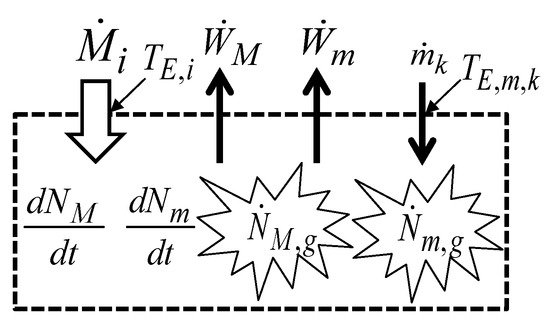
Figure 1.
A schematic representation of the units transfer rate interactions (from left to right: traded merchandise, merchandise wealth, monetary wealth, and monetary exchange) of an economic system.
- -
- Merchandise (goods or services) traded, [U/s]: the number of merchandise units in transit per unit of time (which may be composed of merchandise flow rates [U/s] of different merchandise species i) driven by a potential (economic temperature difference), [U/s] flowing spontaneously in the decreasing economic temperature direction. These are merchandise units that are in the market. The economic temperature at which [U/s] crosses the economic system’s boundary is of major relevance. The economic temperature will be defined in Section 3.1.
- -
- Merchandise wealth, [U/s]: the number of merchandise units in transit per unit of time (which may be composed of merchandise wealth flow rates [U/s] of different merchandise species i) not driven by any potential and thus not being transferred by trading reasons/motivations. These are merchandise units that are not in the market. Consider, for example, a loaded truck, the load being (tradable) merchandise but not the truck itself (which, in this sense, is merchandise wealth). In a different context, the truck can itself be tradable merchandise.
- -
- Monetary wealth, [U/s]: the number of monetary units in transit per unit of time (which may be composed of monetary wealth flow rates [U/s] of different monetary species k) not driven by a potential. These are monetary units not used in the market operations, not being exchanged for merchandise units in the purchasing and selling operations.
- -
- Monetary transfer, [U/s]: the number of monetary units in transit per unit of time (which may be composed of monetary flow rates [U/s] of different monetary species k) not driven by a potential. These are monetary units in the market, used in the market operations and exchanged for merchandise units in the purchasing and selling operations.
Merchandise (tradable) and merchandise wealth (non-tradable) flow rates are merchandise units in transit, which can be material (goods with material existence, labor, hardware) or immaterial (ideas, knowledge, information, software). The monetary flow rates are monetary units in transit, independent of the context and their financial values. They are non-tradable, as their unit prices remain unchanged if transferred or exchanged.
Similarly, as it happens with energy [1,2,3], it is assumed that the number of units of goods, services, and money, in the economic system or crossing its boundary, can be counted by a counter, in the same units [U].
2.3. The Units Balance Equations
Similar to the energy balance equation [1,2,3], an equation can be written setting the balance of the number of units of an economic system, considering the several merchandise (goods and services) and monetary species involved. On a time-rate basis, such an equation states that
A heat reservoir is defined in Thermodynamics as a system whose temperature remains unchanged independently of the heat it receives or releases. A merchandise reservoir is defined similarly as an economic system whose economic temperature (whose concept and meaning are explained in Section 3.1) remains unchanged independently of the merchandise units it receives or releases in trading operations.
In detail, the units balance equation states that the time rate of change of the number of units of all the merchandise species plus the number of units of all the monetary species in the economic system equals the sum of the rates [U/s] of all the traded merchandise species i exchanged by the system (with the NM merchandise reservoirs), minus the merchandise wealth rates [U/s] of all the (non-traded) merchandise species i exchanged by the system, minus the monetary wealth rates [U/s] of all the monetary species k exchanged by the system, plus the input rates [U/s] of all the monetary species k entering the system, minus the output rates [U/s] of all the monetary species k leaving the system, plus the generation rates [U/s] of all the merchandise species i in the system, plus the generation rates [U/s] of all the monetary species k in the system, as
whose reduced form is illustrated in Figure 1. In Thermodynamics, the delivered mechanical work is the positive effect of the thermal engine. This is the reason why the (merchandise and monetary) wealth transfer interactions are positive when released by the economic system, assuming that the positive effect of the economic engine is the delivered wealth. In turn, the (traded) merchandise transfer interactions [U/s] are positive when entering the economic system and negative when leaving it, similar to the heat transfer interactions in Thermodynamics.
It is possible to decompose [U/s] into its components [U/s], [U/s] into its components [U/s], and [U/s] into its components [U/s] associated with each particular merchandise species i. In turn, and similarly, it is possible to decompose the monetary wealth rate [U/s] into its components [U/s] and the monetary generation rate [U/s] into its components [U/s] associated with each particular monetary species k. All the previous decompositions are possible assuming that the involved merchandise rates of every merchandise species i are not coupled with the merchandise rates of any other merchandise species, and that, similarly, the involved monetary rates of every monetary species k are not coupled with the monetary rates of any other monetary species.
Equation (7) can be seen as resulting from the sum of the balance equations for all the merchandise species i
with the balance equations for all the monetary species
Separation of Equation (7) into Equation (8) for all the merchandise species i and Equation (9) for all the monetary species k, respectively, can be conducted, as in the economic processes there are no conversions of merchandise units into monetary units, nor are there conversions of monetary units into merchandise units. What happens in the economic processes are eventual exchanges of merchandise units by monetary units and of monetary units by merchandise units, but not the conversion of the units of one of them into the units of the other.
Even if Equations (8) and (9) can be taken separately, they are coupled, as it is implied that the purchase (income into the economic system) of Mp [U] merchandise units at the unit price [€/U] is associated with the outcome of the mp [U] monetary units, obeying [€], and that the selling (outcome from the economic system) of Ms [U] merchandise units at the unit price ps [€/U] is associated with the income of the ms [U] monetary units, obeying [€], as illustrated in Figure 2. It is through relations such as
that Equations (8) and (9) are coupled in trading operations.
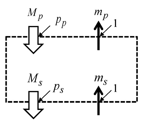
Figure 2.
A schematic representation of the purchase (p) and selling (s) operations, and their associated merchandise and monetary units transfers.
Balance Equations (8) and (9) may themselves be split into a set of balance equations, one for each merchandise species i
and one for each monetary species k
Energy is conserved [1,2,3], but merchandise units and monetary units can, in contrast, be created/generated or destroyed in the economic system. For example, new ideas, new knowledge, or new combinations of goods or services give rise to new (additional) merchandise units without forcedly implying the destruction of an equal number of merchandise units, in which case [U/s]. Situations can exist where some merchandise units are destroyed in the economic system, for example, when plates or glasses are broken in the system, ceasing their existence as plates or glasses in the economic system without implying the generation of an equal number of units of plates or glasses in the system, in which case [U/s]. Another possible situation is, for example, when one new unit (one chair) is generated using 12 wood parts; the 12 wood parts are destroyed in the process (as they cease existing as 12 separated wood parts in the economic system) to the generation of one new unit (one chair) in the system.
Similarly, economic operations can be conducted so that they are associated with the generation of monetary units in the economic system, in which case [U/s], or so that they correspond to the destruction of monetary units in the economic system, cases in which case [U/s]. It must be noted, however, that the generation of monetary units may occur in the central banks only, and that in the common economic operations [U/s]. Monetary units destruction corresponds to melting coins or burning banknotes in the economic system.
[U/s] in Equations (7), (8) and (11) are the sum of negative (received) and positive (released) i merchandise wealth rates exchanged by the economic system through its boundary. Similarly, [U/s] in Equations (7), (9) and (12) are the sum of negative (received) and positive (released) k monetary wealth rates exchanged by the economic system through its boundary.
The units of all the merchandise species i transferred in trading operations with the NM merchandise reservoirs are considered in [U/s]. The merchandise transfer rates can be motivated by trading ( [U/s]) or not ( [U/s]). All the merchandise transfer rates [U/s] motivated by trading and all the merchandise wealth rates [U/s] not motivated by trading are included, respectively, in the first and second terms on the right-hand side of Equations (7), (8) and (11).
The transferred monetary wealth rates [U/s] can have material (tangible, such as coins or monetary billets) or immaterial (intangible, such as cheques or electronic transfers) components. The monetary units exchanged by the economic system are considered separately in Equations (7), (9) and (12) through the terms . They are transferred with no profit purposes, but simply exchanged in the merchandise units purchasing and selling operations.
The common (motivated by profit) economic operations lead to net monetary units accumulation in the economic system ( [U/s]) or to monetary units net income into the economic system ( [U/s]) unless the economic operations are investments and not trading operations.
Multiplying Equation (7) by dt allows obtaining the differential form of the units balance equation for an infinitesimal economic process as
which can be split into two differential equations, one for all the merchandise species i
and the other for all the monetary species k
Symbol d is used for the differential of a property (an exact differential), and symbol δ is used for the differential of a non-property (an inexact differential) [1,2,3].
The differential balance Equations (14) and (15) can themselves be split into a set of differential equations, one for each merchandise species i
and one for each monetary species k
3. The Second Law and the Economic Entropy Balance Equations
There are different ways to introduce the Second Law of Thermodynamics. It can be introduced/set in a structured way [3], starting with the observations of the first thermal engines, invoking the Kelvin–Planck and Clausius statements and using the Carnot relation and the (reversible) Carnot cycle, to arrive at the definition of entropy as a thermodynamic property. Entropy generation emerges as a measure of the irreversibility of thermodynamic processes. Only after that is the entropy balance equation set [3]. Due to space limitations, the required concepts and variables are introduced in this work without demonstration, even if it could be conducted similarly as for Thermodynamics [3]. Similar to the First Law of Economics, the Second Law of Economics is introduced here through the economic entropy (the financial value) balance equation.
3.1. The Meaning of the New Concepts and Variables Involved in the Economic Entropy Balance Equations
One of the properties of an economic system is its economic entropy SE [€] (its financial value). For an economic system composed of NM,i [U] merchandise units of species i, each with its unit price pi [€/U], the economic entropy associated with these merchandise units is
If the same economic system is additionally composed of Nm,k [U] monetary units of species k, each with its exchange rate Fk [€/U], the economic entropy associated with these monetary units is
The economic entropy (the financial value) of the economic system with the [U] merchandise units and with the [U] monetary units is thus
which is the same as Equation (6). It expresses how the economic entropy (the financial value) of the economic system depends on the unit prices of its composing units.
The economic entropy accumulation rate in the economic system is the sum of the merchandise economic entropy and the monetary economic entropy accumulation rates in the system
Usually, individuals and/or corporations strive for positive time rates of change in the economic system’s financial value as composed of the sum of both merchandise financial value and monetary financial value of all the units in the economic system. This corresponds to positive economic entropy accumulation rates in the economic system.
The economic temperature, TE [U/€], of merchandise (goods or services) is defined as the inverse of its unit price p [€/U], that is,
which can be better understood by looking at Equation (70).
The first note on the economic temperature is that its sense is contrary to the usually assumed/referred to in Economics language, stating that the economy is hotter when the unit prices of the traded merchandise are higher.
Temperature is an intensive property of a thermodynamic system, intimately related to its other thermodynamic properties through state equations [3]. Additionally, different particles or chemical species in the thermodynamic system have the same temperature. In turn, the economic temperature proposed here is not a property of the economic system but of merchandise (goods or services), as it depends on the context, which influences its unit price when crossing the economic system’s boundary. From good to good or service to service, their unit prices change, and so do their economic temperatures, even if they compose the same economic system. In the proposed approach, the economic temperature of a merchandise species is relevant, as it influences the economic entropy flow rates entering or leaving the economic system through its boundary. This is why each merchandise flow rate [U/s] of species i is associated with the economic temperature TE,i [U/€] at which [U/s] crosses the economic system’s boundary, as illustrated in Figure 1 and Figure 3. Economic activity is intrinsically related to exchanges and trading operations, which depend on the context conditions. This is why the economic temperature also depends on the context conditions.
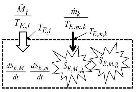
Figure 3.
A schematic representation of economic entropy transfer interactions.
The merchandise economic entropy flow rate associated with the traded merchandise transfer flow rate [U/s] is
which is the merchandise financial value flow rate entering or leaving the economic system through its boundary.
Monetary values have fixed economic entropy (fixed financial values), which do not change in trading operations. The monetary economic entropy flow rates and the merchandise economic entropy flow rates have different natures. The financial value flow rate of the monetary units flow rate [U/s] entering or leaving the economic system is its economic entropy flow rate
Thus, for economic entropy balances, the exchanged monetary units’ flow rates [U/s] can be seen as crossing the economic system’s boundary at the fixed/constant economic temperature [U/€], which does not depend on the context conditions. If the number of monetary units mk [U] is already in euros, Fk = 1 [€/U] and TE,m,k = 1/1 = 1 [U/€].
A merchandise flow rate [U/s] that crosses the system’s boundary at the economic temperature TE = 1/p [U/€] has the associated merchandise economic entropy flow rate [€/s], and a merchandise wealth flow rate [U/s] that crosses the economic system’s boundary has an associated null economic entropy flow rate. Comparing both cases, the merchandise wealth flow rate [U/s] can be seen as a merchandise flow rate crossing the economic system’s boundary at an infinite economic temperature (at a null unit price). In terms of merchandise units, it continues a merchandise wealth flow rate [U/s], and from the merchandise economic entropy viewpoint it has the associated economic entropy flow rate [€/s].
Units of energy from the sun or the wind are available at null unit prices. They are thus available as merchandise wealth. If placed on the market given non-zero unit prices, merchandise wealth is converted into traded merchandise, and (in principle) that traded merchandise will not be converted back into merchandise wealth (into units of energy available at a null unit price). The same happens with natural resources and land (considered before being taken as owned by a proprietary), which are merchandise wealth (available at null unit prices). Imagination, ideas, time, previously acquired knowledge, and writing skills are available for free, at null unit prices, and they are thus available as merchandise wealth. A book can be written at a null unit price, being thus obtained as merchandise wealth. However, once the book is placed on the market, given it a unit price, from the trading operations viewpoint that book is no longer merchandise wealth but traded merchandise.
In common language, it is usual to say that (true) wealth corresponds to things that are not on the market, are not to be purchased or sold, and have no price, or, in the present context, have a null unit price, which is the same as saying that they have an infinite economic temperature.
3.2. The Economic Entropy Balance Equations
Written in the same form as in Engineering Thermodynamics, on a time-rate basis, the economic entropy balance equation states that
It is well known from Thermodynamics that mechanical work flow rates have associated null entropy flow rates. Similarly, wealth (merchandise and monetary) flow rates have null associated economic entropy flow rates. This is why wealth contributions are absent from the economic entropy balance equations.
As illustrated in Figure 3, in detail, the economic entropy balance equation sets that the time rate of change of the economic entropy of all the merchandise species i and of all the monetary species k in the economic system equals the sum of the merchandise economic entropy flow rates [€/s] associated with the merchandise flow rates [U/s] of all the merchandise species i transferred in trading operations by the economic system with the NM merchandise reservoirs, plus the sum of the monetary economic entropy flow rates [€/s] of all the monetary species k entering the economic system, minus the sum of the monetary economic entropy flow rates [€/s] of all the monetary species k leaving the economic system, plus the sum of the merchandise economic entropy generation rates [€/s] of all the merchandise species i in the economic system, plus the sum of the monetary economic entropy generation rates [€/s] of all the monetary species k in the economic system, that is
The entropy balance Equation (25) can be split into two balance equations, one for all the merchandise species i
and the other for all the monetary species k
The reasons legitimating the separation of Equation (25) into Equations (26) and (27) are the same as referred to after Equation (9). Also, in this case, even if Equations (26) and (27) can be taken separately, they are coupled, as referred to in Section 2.3 for the numbers of units. To the purchase (inlet) of Mp [U] merchandise units at the unit price pp [€/U] corresponds the inlet merchandise economic entropy [€] and the associated outlet monetary economic entropy [€], associated with the monetary financial value spent in merchandise purchasing, obeying [€]. To the selling (outlet) of |Ms| [U] merchandise units at the unit price ps [€/U] corresponds the outlet merchandise economic entropy [€] and the associated inlet monetary economic entropy ms/1 = ms × 1 [€], associated with the monetary financial value received from the merchandise selling operation, obeying [€]. It is through relations of the type
that Equations (26) and (27) are coupled. This same result has been anticipated in Equation (10) based on financial arguments, before introducing the economic entropy concept. Divisions and multiplications by 1 are used to highlight that the monetary amount m [U] in euros has the economic entropy [€], which can be written as [€], as the economic temperature of a monetary value in euros is TE,M = 1 [U/€].
It is noted that the banks have business models that take monetary units as merchandise, paying for the use of monetary units in monetary units and charging for the use of those monetary units in monetary units, usually related to the used monetary units through interest rates.
Equation (26) can be split into a set of equations, one for each merchandise species i
and Equation (28) can be split into a set of equations, one for each monetary species k
This can be performed given the meaning of the involved variables, and because there are no crossed relations between them, even if they are coupled through equations of the type of Equation (28).
The economic entropy balance Equations (25)–(27), (29) and (30) can be used for many purposes, including the evaluation of economic entropy generation rates (the financial value generation rates) on the last terms in their right-hand sides, if all their remaining terms are already known.
When comparing to what happens with the Second Law of Thermodynamics [1,2,3], for which irreversibility and entropy generation are associated with the imperfection of the thermodynamic system’s operation, the developed and proposed economic Second Law states that the economic irreversibility, or economic imperfection, of the economic systems’ operation is associated with the economic entropy generation (the financial value generation). This will be explored in more depth later.
Multiplying Equation (25) by dt allows obtaining the differential form of the economic entropy balance equation for an infinitesimal process as
which can be split into two differential equations, one for all the merchandise species i
and the other for all the monetary species k
Equation (32) may be split into a set of differential equations, one for each merchandise species i
and Equation (33) can be split into a set of differential equations, one for each monetary species k
Some final notes must be added to this section. The first one to clarify that
and that
as the exchange rate Fk [€/U] of each of the monetary units remains unchanged, and the monetary economic entropy of the Nm,k [U] monetary units is its financial value, Nm,k · Fk [€].
The second is that in common trading operations, the merchandise economic entropy flow rates are balanced by the exchanged monetary economic entropy flow rates involved in the purchasing and selling operations, thus implying that
For those cases, Equation (25) is simplified to give
It needs to be noted that Equation (38) sets a relation between terms of the economic entropy balance equation involving the merchandise species i and the monetary species k, leading to a simplified version (Equation (39)) of the original economic entropy balance Equation (25). Due to that, in any subsequent developments based on Equation (39), the terms involving the merchandise species i can no longer be separated from those involving the monetary species k. As there is no monetary units generation or destruction in the common trading operations, [€/s], and as , Equation (39) can be rewritten as
which can be read as follows: the monetary financial value accumulation rate is equal to the merchandise economic entropy generation rate minus the merchandise economic entropy accumulation rate, all of them in the economic system.
3.3. Merchandise Transfers Motivated by Trading and Arbitrary Decisions
Any thermodynamic process, spontaneous or not, occurs with associated energy transfer interactions, with the consequent positive entropy generation [1,2,3], which is null in the ideal limit reversible process. Thermodynamic properties of the system change in the process according to the equation of state, and no room exists for arbitrariness.
When dealing with economic processes, if they occur naturally, motivated by trading, as the merchandise transfers occur naturally from higher economic temperatures to lower economic temperatures (from lower unit prices to higher unit prices), the resulting economic entropy generation (the resulting financial value generation) is positive, or null in the limit of economic reversibility. However, arbitrary decisions are usual when dealing with economic processes. These may be in the same direction as the natural trading processes, leading to positive economic entropy generation, or in the inverse direction, resulting in negative economic entropy generation.
A negative economic entropy generation sounds strange, even impossible to occur, given the positivity of entropy generation in Thermodynamics [3]. The controller of the economic system, and thus also of the economic processes, may make arbitrary decisions. They can be contrary to the natural economic processes as defined in the present context (those motivated by trading, with positive, or in the economically reversible limit null, economic entropy generation). Those processes can thus have associated negative economic entropy generation (negative financial value generation). In contrast, in Thermodynamics, no arbitrary decisions can be taken concerning entropy generation, energy transfer interactions inducing changes in the thermodynamic system’s properties that always lead to positive, or in the ideal reversible limit null entropy generation.
Energy (mechanical work) needs to be invested for the occurrence of a non-spontaneous process. This may not be the case in Economics, as non-natural economic processes may happen based on arbitrary decisions, without investing merchandise wealth for that.
3.4. Naturally Driven Economic Operations and Arbitrary Decisions
Economic operations can be trading operations, naturally driven by an economic temperature difference or arbitrary decisions made by the economic system controller. Consider an economic system with [U] units, where [U] is the total number of merchandise units (involved in trading operations and taken as wealth, respectively), and [U] is the total number of monetary units (exchanged in trading operations and taken as wealth, respectively) in the system. The wealth merchandise units (NM)W [U] and monetary units (NM)W [U] are set aside and are not involved in the trading operations in which the economic system participates. This is illustrated in Figure 4.
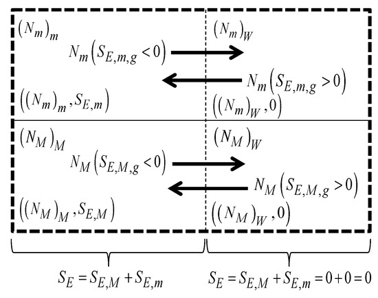
Figure 4.
Economic system as formed of four parts: one (top left) with monetary units involved/exchanged in trading operations and their corresponding monetary economic entropy; another (top right) with monetary units set aside as monetary wealth, not involved/exchanged in trading operations, and thus with null monetary economic entropy; another (down left) with merchandise units involved in trading operations and their corresponding merchandise economic entropy; and another (down right) with wealth merchandise units set aside, not involved in trading operations, with null merchandise economic entropy.
The (NM)W [U] wealth merchandise units have a null merchandise economic entropy; however, they have a non-null potential financial value as, if they are placed on the market, giving them a non-zero unit price, they have a non-zero merchandise economic entropy (non-zero financial value). The economic system’s controller may make the arbitrary decision to move the NM [U] merchandise units from the bottom left to the bottom right or from the bottom right to the bottom left of Figure 4. If it makes the arbitrary decision to move the NM [U] merchandise units from the bottom left to the bottom right of Figure 4, that corresponds to internally, in the economic system, convert merchandise that was in the market, with the merchandise economic entropy [€], to merchandise wealth, this out of the market, corresponding to decrease the merchandise economic entropy of the system by NM · p [€]. Such an arbitrary decision corresponds to the negative economic entropy generation [€] in the economic system. If the controller makes the arbitrary decision to move the NM [U] merchandise units from the bottom right to the bottom left of Figure 4, a symmetrical effect occurs. The merchandise economic entropy (the merchandise financial value) of the economic system depends thus on the arbitrary decisions made by the economic system’s controller.
Similar considerations can be made considering the monetary units in the economic system. The (Nm)W [U] monetary units have null monetary economic entropy, but they have a non-null potential financial value as they can be placed on the market and involved/exchanged in the trading operations, with a non-zero monetary economic entropy (non-zero financial value). The economic system’s controller may make the arbitrary decision to move the Nm [U] monetary units from the top left to the top right or from the top right to the top left of Figure 4. If it makes the arbitrary decision to move the Nm [U] monetary units from the top left to the top right of Figure 4, that corresponds to internally, in the economic system, convert monetary units that were in use in trading operations, with the monetary economic entropy Nm × 1 [€], to monetary units taken as wealth, with a null monetary economic entropy, set aside and out of use in the trading operations. This corresponds to a decrease in the monetary economic entropy of the system by Nm × 1 [€]. Such an arbitrary decision thus corresponds to the negative monetary economic entropy generation [€] in the economic system. If the controller makes the arbitrary decision to move the Nm [U] monetary units from the top right to the top left of Figure 4, a symmetrical effect occurs. The monetary economic entropy (the monetary financial value) of the economic system depends thus on the arbitrary decisions made by the economic system’s controller.
The pocket money we have for use in our daily purchases is not usually taken as monetary wealth. In contrast, the money set aside in the bank or invested in financial products, which is not in use or intended to be used in our daily purchases, is taken as monetary wealth. Money does not lose its financial value when taken as monetary wealth, maintaining its potential financial value, as it can easily change from being considered monetary wealth to being available for use in trading operations. Similarly, the merchandise the merchant puts on the market is considered merchandise to be traded; however, its house and car, out of the market, are not considered merchandise, but instead detained as merchandise wealth. However, they may be taken as tradable merchandise and placed on the market. When detained as merchandise wealth, they have no financial value (they have null unit prices). Still, they have a potential financial value revealed when they are taken as merchandise placed on the market, giving them non-zero unit prices.
It is thus clarified that if there are merchandise transfer operations that are naturally driven by trading purposes, some other economic operations may depend only on arbitrary decisions of the economic system’s controller. These arbitrary decisions can go in the same direction as the naturally driven trading operations, or they can go in the inverse direction. Another arbitrary decision is to maintain some merchandise units on the market and take some other merchandise units as merchandise wealth out of the market.
In Thermodynamics, arbitrary decisions are taken over the energy transfer interactions, and (always positive, or in the ideal reversible limit null) entropy generation is a consequence. The energy transfer interactions occur first (the cause), and the entropy generation occurs as a result (the consequence). Natural (motivated by trading) economic operations and arbitrary decisions are taken considering economic entropy first (the cause), whose generation can be positive or negative, or in the ideal economically reversible limit null, and the (merchandise and monetary) units transfer interactions are the result of that (the consequence).
Entropy is not a familiar concept, sounding strange and only understood by experts; Thermodynamics helps to define, clarify, demystify, and quantify it. In contrast, economic entropy (financial value) is a familiar concept, associated with everything in everyone’s daily life, all of us being proficient and experienced economic entropy accountants, analysts, and decision-makers.
3.5. End User and Final Consumer
If a person or a corporation purchases a goods or a service and is its end user, the (NM)M [U] merchandise units purchased at the unit price p [€/U] have the merchandise economic entropy (the merchandise financial value) (NM)M· p [€]. The end user is retiring those merchandise units from the market, taking them as merchandise wealth, taken as (NM)W = (NM)M [U]. Even taken as merchandise wealth, set aside from the market, those merchandise units continue retaining their potential financial value (NM)M· p [€]. This process, as illustrated in Figure 5a, has thus the negative merchandise economic entropy generation (the negative merchandise financial value generation)
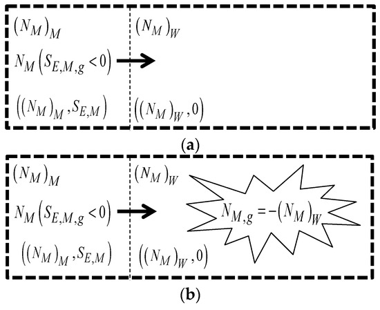
Figure 5.
A graphical illustration of the economic processes corresponding to (a) end use and (b) final consumption.
If that number of merchandise units (such as a car or a pair of shoes) is used by the final consumer, the number of wealth merchandise units (NM)W [U] is maintained in the economic system and is not destroyed. However, its potential financial value is continuously reducing by wearing and aging, which corresponds to a continuous decrease of its potential unit price, thus leading to continued negative merchandise economic entropy generation (continued negative merchandise financial value generation). A continued reduction of the potential unit price corresponds to a continued increase in the economic temperature, contrary to the spontaneous economic processes motivated by trading. If the good is an antique, the inverse usually occurs, with its unit price continuously increasing as it ages.
If a person or a corporation purchases a good and is its final consumer, the merchandise units (NM)M [U] acquired at the unit price p [€/U] have the merchandise economic entropy (NM)M· p [€]. As it is the final consumer, it is retiring those merchandise units from the market, taking them as merchandise wealth, obeying (NM)W = (NM)M [U]. To that process corresponds the negative merchandise economic entropy generation as given in Equation (41). If, after those wealth merchandise units are consumed or, in the present context, destroyed, it is
This is what happens when a bottle of wine is firstly purchased as traded merchandise, then retired from the market to be detained as merchandise wealth, and after that is drunk, corresponding to both negative merchandise economic entropy generation and negative merchandise units generation in the economic system.
Both cases of the end use or final consumption lead to negative merchandise economic entropy generation in the economic system. However, they must have been preceded by some economic operations in which individuals or corporations that are the end users or final consumers obtained the monetary units required to purchase the merchandise of which they are the end users or the final consumers. That is, before the end use or the final consumption, some economic processes existed with associated positive monetary economic entropy accumulation higher than, or in the limit reversible situation equal to, the negative economic entropy generation associated with the end use. The overall process results thus in an overall positive or, in the limit reversible situation, null merchandise economic entropy generation, even if the positive economic entropy generation or accumulation phases occurred before (in time) the negative merchandise economic entropy generation phase.
3.6. Some Challenging Reflections
The ways of thinking and decision-making when dealing with energy (thermodynamic) systems are essentially First-Law based, using the notions of mass and energy balance equations, and mass and energy efficiency. Only after that, and left to the experts, are the thinking and decisions based on the Second Law, usually using the entropy generation minimization criterion [26] and/or the exergy analysis and exergy efficiency [1,2,3]. Contrarily, the ways of thinking and deciding when dealing with economic systems are essentially economics Second-Law based, using the (naturally acquired) notions of economic entropy (financial value) balance equation and economic entropy (financial value) efficiency. Only after that are the thinking and decisions implemented based on the First Law of Economics, usually using the units balance equations notion.
Some kinds of evolution and change may occur in the ways of thinking and decision-making, remaining to be clarified, discussed, and discovered if they must effectively occur. Some of the questions to consider are as follows:
- -
- Should thermodynamic thinking and decision-making be based increasingly more on the Second Law and less on the First Law? The work by Bejan [26] is a remarkable contribution in that direction, as well as the progress of the Second Law analysis [3] (emphasis on entropy rather than on energy).
- -
- Should economic thinking and decision-making be based increasingly more on the First Law of Economics and less on its Second Law? In some ways of life, such as those of small farms and villages, exchanging products with the neighbors, helping each other free of charge, sharing tools, manpower, and non-paid labor, exchanging goods and avoiding purchasing and selling, thus avoiding using money and trading operations, are efforts in that direction (emphasis on the number of units rather than on economic entropy and financial value).
- -
- Should the entropy generation minimization criterion be taken as the headlight of both Thermodynamics and Economics?
- -
- Merchandise transfers (First Law of Economics) in trading operations have their associated merchandise economic entropy transfers (Second Law of Economics), which have their associated monetary economic entropy transfers and their respective monetary units transfers (a third species involved in the trading operations). Heat transfers (First Law) have their associated entropy transfers (Second Law), but there is no third species involved to reward the entropy donor and receive from the entropy receiver. Entropy transfers seem to be intangible and not accompanied by any species of entropic money. Should we set ‘thermy’ as the thermodynamic analog of money in Economics to reward the entropy donor and receive from the entropy receiver, to pay for the received entropy?
- -
- Banks have business models based on monetary financial values, that is, based on monetary economic entropy. Perhaps in the future, they, or other organizations, will have their analog business models based on (thermodynamic) entropy, using entropic counters and ‘thermies’.
These are some examples of challenging reflections from which Economics may benefit when using the perspective of Thermodynamics, and from which Thermodynamics may benefit when using its Economics analogs.
3.7. Concluding Remarks
For simplification purposes, only monetary units in euros will be considered in the following section, with the associated economic temperature TE,m = 1 [U/€]. Even thus, monetary economic entropy balance Equation (27) cannot be obtained by multiplying monetary unit balance Equation (9) by F1 = 1 [€/U], as the monetary wealth is present in Equation (9) but absent from Equation (27). This can only be the case if the monetary wealth transfer interactions are null.
As a given economic temperature is related to a given merchandise species, for simplification purposes, in the sections that follow only one merchandise species will be considered. For more than one merchandise species, the addition of the contributions of the different merchandise species must be made for the whole (composed) economic system.
The thermodynamic and economic processes for which the respective entropy generations are null, are ideal limits that exist only in our minds and in academic studies, and, in this sense, they seem to be utopic. However, they are of major importance, as they give us the directions to follow towards improved perfection and reversibility, even if they are not attainable under real conditions.
4. Trading as Merchandise Exchange for Money
This section analyzes the purchasing, selling, and trading operations and their associated monetary exchanges using the perspective of Thermodynamics.
4.1. Purchasing Process
In a purchasing process, the economic system receives Mp [U] merchandise units and releases |mp| [U] monetary units, as illustrated in Figure 6a.
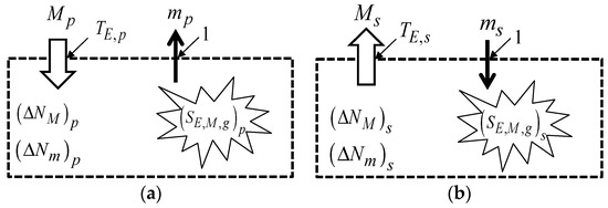
Figure 6.
Economic operations involving the exchange of merchandise for money: (a) purchasing and (b) selling.
The application of Equations (16) and (17) and of Equations (29) and (30) to the economic system in Figure 6a, once integrated to consider the whole purchasing process, gives, respectively,
Merchandise and monetary economic entropy balance Equations (45) and (46) are coupled, as [€].
For an economic system composed of merchandise and monetary units, adding Equations (45) and (46) side by side leads to
As the Mp [U] merchandise units enter the economic system at the unit price pp [€/U], there is no merchandise economic entropy generation in the purchasing process, and [€].
4.2. Selling Process
The application of Equations (16) and (17) and of Equations (29) and (30) to the economic system in Figure 6b, once integrated to consider the whole selling process, gives, respectively,
Merchandise and monetary economic entropy balance Equations (50) and (51) are coupled given that [€].
Adding Equations (50) and (51) side by side leads to
As the [U] merchandise units leave the economic system at the unit price ps [€/U], there is no merchandise economic entropy generation in the selling process, and [€].
4.3. Trading Process
The whole trading process, including purchasing followed by selling, seems to be accounted for, in principle, adding the equations corresponding to the separated purchasing and selling processes. There is, however, a subtle yet crucial step/process that needs to be considered between the purchasing and selling processes. It corresponds to the decision to increase the unit price of the sold [U] merchandise units from pp [€/U] to ps [€/U], which is the same as decreasing their economic temperature from Tp = 1/pp [U/€] to Ts = 1/ps [U/€], Ts < Tp [U/€], in the economic system. This intermediate step/process corresponds thus to the [€] increase of merchandise economic entropy in the economic system. Table 1 summarizes the so-obtained results.

Table 1.
Changes in the merchandise units, monetary units, merchandise economic entropy, monetary economic entropy, and the merchandise economic entropy generation in the processes composing a trading operation.
In a trading operation (last column of Table 1), merchandise economic entropy increases by [€], corresponding to the [U] merchandise units that entered the economic system at the unit price pp [€/U] without leaving the economic system. The monetary economic entropy increases by [€], corresponding to the change [U] on the monetary units in the economic system. A net monetary financial gain could be obtained or not, depending on the number of merchandise units purchased and sold. For a positive monetary economic entropy change in the economic system (a positive monetary financial gain), it must be [U], and the number of merchandise units sold must be [U].
4.4. Trading with Null Economic Entropy Generation
A possible limit situation is that corresponding to the selling of the [U] merchandise units in such a way that there is no monetary economic entropy change in the system, [€]. As [€] and [€]; this situation corresponds to selling the [U] merchandise units. The merchandise economic entropy generation corresponding to this situation is
The dimensionless factor [-], which can be referred to as the economic Carnot factor, is common when dealing with economically reversible processes, as will be seen in Section 5.2.
The merchandise economic entropy of the purchased and non-sold [U] merchandise units, which entered the economic system at the unit price pp [€/U], is equal to the merchandise economic entropy generation in the trading process as given in Equation (53). Thus, if the non-sold [U] merchandise units in the economic system are taken as merchandise wealth, a decision that corresponds to the negative merchandise economic entropy generation that is symmetrical to that in Equation (53), no net merchandise economic entropy generation exists in the economic system. No merchandise and monetary economic entropy generation exists in the economic system in such a process, which is thus referred to as the economically reversible trading operation.
For the (general) complete trading operation, the obtained monetary units [U], with [€] were obtained, which can be taken as the monetary wealth increase in the economic system. Some of their financial value, [€], can be retained as monetary wealth in the economic system, and the remaining [€] be used to purchase the [U] merchandise units at the purchasing unit price pp [€/U]. As the [U] monetary units were obtained as monetary wealth, the [U] retained monetary units are monetary wealth, and the purchased merchandise units [U] can be taken as merchandise wealth, both in the economic system. This can be written as
4.5. Trading Operations Involving Services
In what follows, the services (labor, electricity, communications, cleaning, security, etc.) required in real trading operations are considered. Two different cases are taken into account: one in which all the services are purchased, including labor (Figure 7a), and one in which manpower (labor) is generated in the economic system (Figure 7b).
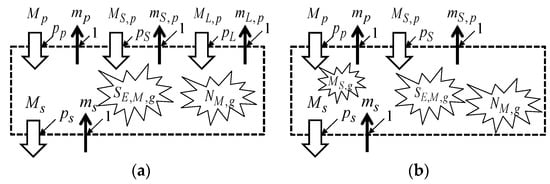
Figure 7.
Trading operation: (a) purchasing all the required services, including labor; and (b) purchasing part of the services, including the generation of the required labor units in the economic system.
In the first case, represented in Figure 7a, Mp [U] merchandise units are purchased at the unit price pp [€/U], and are sold the [U] merchandise units at the unit price ps [€/U], with the associated [U] and ms [U] monetary unit exchanges, respectively. The merchandise trading process requires the purchase of the MS,p [U] units of services (treated as other merchandise) at the unit price pS,p [€/U], and of the ML,p [U] units of labor (treated also as merchandise) at the unit price pL,p [€/U]. The unique useful result of the trading operation is the selling of the [U] merchandise units at the unit price ps [€/U], receiving the corresponding ms [U] monetary units.
Merchandise unit balance Equation (8) and monetary unit balance Equation (9), once integrated to apply to the whole trading process, give, respectively,
where [U], as the services and labor units are consumed (destroyed) in the trading process, and thus [U].
Merchandise economic entropy balance Equation (26) and monetary economic entropy balance Equation (27), once integrated to apply to the whole trading process, give, respectively,
The above merchandise and monetary economic entropy balance equations are coupled given that
All the units of services, including labor, purchased as merchandise, are destroyed in the economic system, thus leading to the corresponding negative merchandise economic entropy generation in the economic system. For the trading operation’s financial sustainability, this negative merchandise economic entropy generation must be balanced, or even surpassed, by a positive economic entropy generation, which is achieved by increasing the selling unit price ps [€/U] as required for that purpose.
If the objective of the trading operation is a positive change in the monetary economic entropy (monetary financial profit), according to Equation (56), it must be [U], which is the same as saying, using Equation (58), that it must be [€]. If the objective of the trading operation is a positive change in the merchandise economic entropy in the economic system, according to Equation (57), it must be [€]. If the objective of the trading operation is a positive change in both the monetary and merchandise economic entropies, it must be, simultaneously, [€] and [€]. In any case, this results in conditions over the number of units and unit prices of the purchased and sold merchandise, and over the number of units of services purchased and their unit prices. This is the conventional economic way of thinking: start with the economic Second Law balance equations and then act based on the economic First Law balance equations to obtain the expected Second Law results.
For the second case, schematically represented in Figure 7b, the required units of labor are not purchased but instead generated in the economic system. Elements such as time, knowledge, expertise on the product, etc., which can be available for free, at null unit prices, can be seen as merchandise wealth. In this case, the NM,L,g [U] units of labor required for the trading operation are generated free of charge in the economic system and later destroyed (to conduct the trading operation) in the economic system. If the generator of these labor units does not require to be paid for them, the earlier analysis performed for the case in Figure 7a can be conducted considering ML,p = 0 [U]. However, if the generator of these labor units wants to be paid for them, the analysis made for the case in Figure 7a may apply considering ML,p = NM,L,g [U]. However, there is a subtle difference between these two cases. In the first case, the ML,p [U] labor units entered the economic system and were destroyed in the economic system, which led to the associated negative merchandise economic entropy generation. In the second case, the ML,p = NM,L,g [U] labor units were initially generated in the economic system as merchandise wealth, with an associated null merchandise economic entropy generation, but when they were further treated as merchandise, giving them the unit price pL,p [€/U] of the labor units, it corresponded to a positive merchandise economic entropy generation in the economic system.
The more usual trading operation is schematically illustrated in Figure 7a. A more perfect trading operation can be conducted by selling the merchandise at a unit price equal to the purchasing unit price, selling the units of services as merchandise at unit prices equal to their purchasing unit prices, and paying the trader only by the units of labor it spends in the trading operation at the unit price pL,p [€/U]. In the limit situation, the trader does not want to be paid for the units of labor it spends in the trading operation, and no economic entropy generation exists in such an ideal reversible (with no economic entropy generation), and thus perfect, trading operation. The situation when the trader is not acting to obtain profit but just to be paid for the labor units spent rewards the fair value to the trader and leads to the lowest economic entropy generation in the trading operation. Once again, thinking firstly based on the economic Second Law balance equation, and acting secondly based on the economic First Law balance equation to reach the objectives set by the economic Second Law.
The usual trading operations consider rates, or commissions, to obtain the selling unit price from the purchasing unit price. As the purchasing unit price includes the costs of the units of services involved in the previous stages of the trading operation chain, those rates are applied to both the unit price of the merchandise as such and the unit prices of services involved in the previous stages of the trading chain. This leads to higher selling unit prices than the previous model, referred to as more perfect, with no profit purposes, generating less economic entropy.
Once a product is produced/transformed/manufactured, it has a base unit price. The stages of the trading chain do not change the product and do not add anything to the product. Thus, they must not change the unit price of the product itself. What can be added by the successive stages of the trading chain are the costs of the units of services required at those stages. In this sense, and contrary to what is commonly said, it is argued that the trading of products and services does not add value to them but only increases their unit prices. When purchasing 1 kg of rice at a given unit price, we do not know how much corresponds to the 1 kg of rice base price and how much corresponds to the cost of the services involved in all the steps of the trading chain from its production and packing up to supermarket display. The trading chain generates merchandise economic entropy (merchandise financial value), resulting in increased selling unit prices, without adding intrinsic value to the traded merchandise.
4.6. Services as Economic Friction/Viscosity
The friction-generated heat originates from lost mechanical work and can thus be seen as generated at an infinite temperature. This heat flows naturally from that infinite temperature to any (finite) local boundary temperature where it leaves the thermodynamic system.
Some service units are required for the occurrence of any economic operation, and monetary units are required to pay for those service units. The main objective of the merchandise trading process is to sell merchandise units, and not to purchase service units. The part of an economic operation that corresponds to the service units purchase required for that is schematically illustrated in Figure 8. It includes the purchase of MS,p [U] service units (taken as merchandise) at the unit price pS [€/U]. The monetary units [U] leave the economic system to pay for these service units, obeying [€]. The [U] monetary units leaving the economic system for that purpose must be balanced by an equal number of monetary units [U] entering the economic system as a result of selling the [U] merchandise units at the unit price ps [€/U] for that purpose, obeying [€]. As the economic temperature TE,s [U/€], at which the [U] merchandise units are sold to obtain the monetary units required to pay for the required service units is unknown, the merchandise for that purpose must enter the economic system as merchandise wealth, at an infinite economic temperature. According to Figure 8, invoking the merchandise units balance Equation (8), it must be [U]. As these [U] wealth merchandise units enter the economic system at an infinite economic temperature, they naturally flow to any other finite economic temperature TE,s [U/€] at which they leave the economic system as merchandise sold. It is noted that the MS [U] service units entering the economic system cease their existence after contributing to the economic operation occurrence, being thus destroyed in the economic system, and [U].
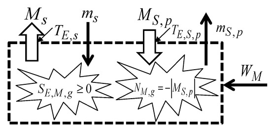
Figure 8.
Schematic representation of friction in economics.
The application of merchandise units balance Equation (8) and monetary units balance Equation (9) to the economic system in Figure 8, once integrated to consider the whole process (assuming that no merchandise nor monetary storage exists in the economic system) leads, respectively, to
As [U], Equation (60) gives that [U], that is, the [U] merchandise units entering the economic system as merchandise wealth are equal to the number of merchandise units [U] sold at the unit price ps [€/U]. In turn, Equation (61) sets that the number of monetary units involved in the purchasing of the MS,p [U] service units is the same as that involved in the selling of the [U] merchandise units.
The application of merchandise economic entropy balance Equation (26), once integrated to consider the whole process, leads to
and since [€], [€], and [U], it is
and no merchandise economic entropy exists in the analyzed process, considering the compensation of the purchase of service units (as merchandise) by selling some of the merchandise units previously obtained as merchandise wealth.
Friction always leads to positive entropy generation, since no negative heat generation occurs. However, negative generation of merchandise units may occur in the economic systems, corresponding in the present context to the destruction of the service units in the economic system, contributing to a negative merchandise economic entropy generation in the economic system.
The monetary financial result that could be obtained from selling the [U] merchandise units would result in a monetary financial gain, which in this case is lost as it is used to purchase the required service units that are later destroyed in the process.
Once services are understood as the economic friction of the economic operations, with the cost of the required units of services for their occurrence, MS,p · pS,p [€], the losses by economic friction will decrease as this product decreases.
This can be accomplished by decreasing the service unit prices, the limit being the case when no payment is required for these service units. This is, for example, the case of the units of labor associated with volunteer (non-paid) work, self-services at restaurants, gas stations, and other shops, and customer wrapping of Christmas presents in shops and supermarkets. Another way is to reduce the service units required for a given economic operation. Processes increasing automation and automatization, reducing human labor, bringing the producers and the customers closer to reducing transportation costs, electronic commerce with reduced direct human intervention, and pay points with no human operators are examples in that direction. An interesting case is the IKEA business model: the packaging of disassembled furniture is mainly of a parallelepiped shape, reducing volume and the cost of transportation services; transportation from the stores is conducted by the customer without remuneration; and the furniture is assembled by the customer at home, again without remuneration. All these examples correspond to the use of some of the customers’ time and skills, which are not remunerated (corresponding to the use of merchandise wealth—in this case, non-paid labor—obtained at null unit prices from the customers). As the purchased products are cheaper as a result, such types of business models include one ‘hidden’ part that corresponds to the direct exchange of products (from the seller) for services (from the customer), with no money involved in that exchange operation, which is part of a more global trading operation. Avoiding the use of money in trading operations, making direct exchanges of products and services, and reducing the involved unit prices are ways to act toward the increased reversibility of economic operations, and, consequently, decreased economic entropy generation. This is the way toward a more perfect (more reversible) economy.
4.7. Additional Notes on the Generation of New Units and Their Introduction to the Market
The new NM,g > 0 [U] merchandise units generated in the economic system are generated as merchandise wealth, having thus a null financial value. The application of merchandise units balance Equation (11) and merchandise economic entropy balance Equation (29) to the process corresponding to the generation of the new merchandise units in the economic system gives, respectively,
since the NM,g [U] generated merchandise wealth units do not generate merchandise economic entropy in the system.
If the new NM,g [U] generated wealth merchandise units are introduced into the market, giving them the finite unit price ps [€/U], this step corresponds to maintain the same number NM,g [U] of merchandise units in the economic system, and the application of the merchandise economic entropy balance Equation (29) to this process gives
as the merchandise financial value of the NM,g [U] merchandise units in the economic system increases by NM,g · ps [€] in this step.
If, after that, the NM,g [U] merchandise units are sold at the ps [€/U] unit price, the application of unit balance Equation (11) and merchandise economic entropy balance Equation (29) to the selling process gives, respectively,
As for the selling process it is [€], Equation (68) shows that the merchandise economic entropy generation [€] in the selling process is null.
For the whole process, the addition of Equations (64) and (67) gives that [U], and the addition of Equations (65), (66) and (68) sets that [€], and no merchandise economic entropy generation exists in the whole process. This would be the anticipated result, as the economic system started with 0 [U] and ended with 0 [U] merchandise units.
Looking at what happened to the monetary units, nothing happened in the step corresponding to the NM,g [U] wealth merchandise units generation or in the step corresponds to put the NM,g [U] wealth merchandise units generated in the market, but the inlet of the ms [U] monetary units in the economic system corresponded to the selling operation. The application of monetary economic entropy balance Equation (30) to the selling process gives
obeying [€].
The whole process of generating the NM,g [U] wealth merchandise units in the economic system, their introduction in the market at the unit price ps [€/U], and their selling at the unit price ps [€/U], result thus in the ms [U] monetary units and the monetary economic entropy ms × 1 [€] incomes into the system. The number of merchandise units in the economic system has not changed in the whole process, but the number of monetary units in the economic system has increased by ms [U]. This corresponds to the monetary financial gain of ms × 1 [€] resulting from such a process. This is how the generation and selling of new merchandise units may lead to monetary financial gain.
If not all the NM,g [U] generated merchandise units are sold, only the merchandise units that are sold must be considered in the introduction to the market step, and only that number of merchandise units must be considered in the selling operation step.
If the NM,g [U] merchandise units, generated as merchandise wealth in the economic system, remain in the economic system as merchandise wealth, only a change (increase) of NM,g [U] occurs in the number of merchandise units in the system, but not in the number of monetary units, the merchandise economic entropy, and the monetary economic entropy of the economic system. Even so, those NM,g [U] merchandise units detained as merchandise wealth in the economic system have a potential merchandise economic entropy (a potential financial value) that is NM,g · ps [€], since ps [€/U] is the realistic unit price of these merchandise units if they are to be introduced in the market and sold.
Merchandise transfer occurs naturally from the higher economic temperatures (from the lower unit prices) to the lower economic temperatures (to the higher unit prices), yet no rule has been set for that, and arbitrary decisions may be made by the economic system’s controller for non-natural operations occurring in the inverse direction. Even so, it is usual for governments and/or other regulatory authorities to set penalties for the traders that operate in the market in the non-natural direction, selling merchandise at unit prices smaller than those at which they were purchased, that is, forcing the merchandise trading in the non-natural increasing economic temperature direction. Trading in the decreasing economic temperature direction or increasing unit prices direction is a natural law, but not a physical law, with punishments for those violating it. In a certain way, it is thus a Law imposed by the Law and verified by the Law, with non-compliance punishable by the Law.
Another factor to bear in mind is that any tendency to decrease the economic entropy generation in trading operations leads to the retention of wealth merchandise and monetary units in the economic system. If they were used in further trading operations that resulted in positive economic entropy generation. In practice, and in simpler terms, this corresponds to increased savings (goods and money), and reduced goods trading (commerce) and consumption. It is not being argued that this is the way to be followed; what is being argued is that this is the way leading to a decreasing economic entropy generation, and thus to a more perfect economy in the present context. It can also be said that the annual positive, and expectedly high, growth rates that governments and countries like to announce are intrinsically related to the annually increasing economic entropy generation (annually increasing financial value generation), and thus to less-perfect and more irreversible economies.
5. Merchandise Transfer through an Economic Temperature Difference
Heat transfer through a finite temperature difference, and the associated generated entropy, is of major relevance in Engineering Thermodynamics. Merchandise trading is of major relevance in Economics and is analyzed as merchandise transfer through an economic temperature difference and the associated generated economic entropy. Balance equations are considered on a time-rate basis, which is the most useful one for the intended purposes.
5.1. Merchandise Transfer through a Finite Economic Temperature Difference
The process under analysis is schematically represented in Figure 9, consisting of the steady merchandise transfer flow rate [U/s] through the economic temperature difference [U/€], [U/€].
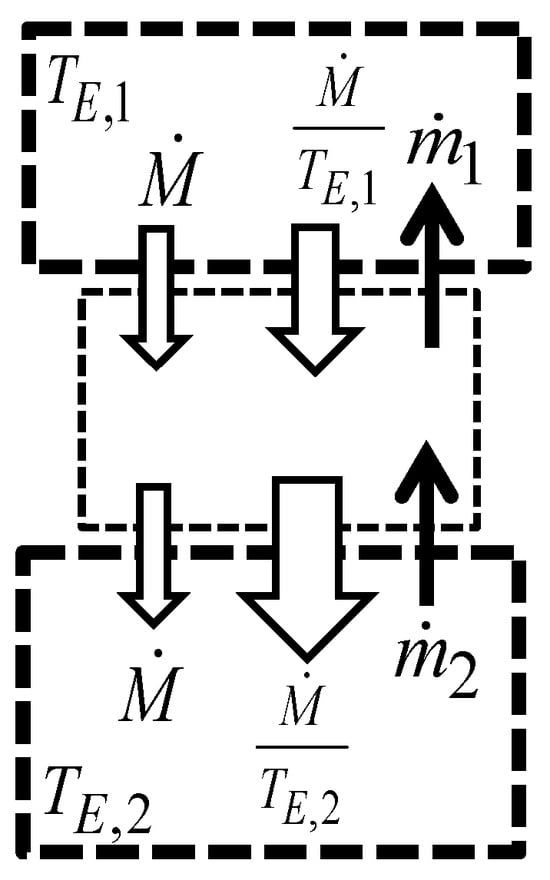
Figure 9.
Merchandise transfer process through a finite economic temperature difference.
Merchandise units balance Equation (11) and merchandise economic entropy balance Equation (29) applied to the economic system sandwiched between the TE,1 [U/€] and TE,2 [U/€] merchandise reservoirs in Figure 9 give, respectively, [U/s] and [€/s]. The merchandise economic entropy flow rates entering and leaving the economic system are [€/s] and [€/s], respectively, and the merchandise economic entropy generation rate is
It is unknown how the economic temperature changes in the economic system, between different parts of its boundary, the merchandise economic entropy generation occurring elsewhere in the economic system.
The merchandise flow rate [U/s] is traded, purchased at the unit price [€/U], and sold at the unit price [€/U], p2 > p1 [€/U]. The rate of profit generation (rate of financial value generation) in the trading operation, which is the same as the merchandise economic entropy generation, as given in Equation (70), is a different way to look at a well-understood and familiar result from the economic viewpoint: the financial profit rate obtained from the trading process is the product of the merchandise flow rate traded by the difference between the selling and purchasing unit prices.
Equation (70) is the main result leading to the definition of the economic temperature as the inverse of the unit price, as anticipated in Equation (22). Considering a Society familiar with the numbers of units, with units [U], and with the economic entropy with units [€], but not with the economic temperature TE [U/€], it can be learned from Equation (22) that the units of the economic temperature are 1/[€/U] = [U/€].
Monetary units balance Equation (12) and monetary economic entropy balance Equation (30) applied to the economic system sandwiched between the TE,1 [U/€] and TE,2 [U/€] merchandise reservoirs in Figure 9 give, respectively,
Equations (71) and (72) are coupled through the conditions
The economic system sandwiched between the TE,1 [U/€] and TE,2 [U/€] merchandise reservoirs in Figure 9 operates steadily from the merchandise point of view, thus being [U/s] and [€/s]. The monetary flow rate [U/s] entering the economic system is higher than the monetary flow rate [U/s] leaving it, thus leading to a positive accumulation rate of monetary units in the economic system, [U/s], with the associated positive accumulation rate of monetary economic entropy in the economic system, [€/s]). This is the same as saying that the trading operation leads to a positive accumulation rate of monetary financial value in the economic system.
It can now be better understood that the economic temperature is not a property of the economic system as is the case with temperature in Thermodynamics. Economic temperature, the inverse of the unit price, depends on the context, which conditions the unit prices of the traded merchandise. It is also clearer that the relevance of the economic temperature is mainly on how it influences the merchandise economic entropy flow rates (the merchandise financial value flow rates) entering and leaving the economic system.
In this case, and contrary to what happens with heat transfer, no deterministic laws exist relating the merchandise transfer flow rate to the economic temperature difference [U/€], [U/€], or to the unit price difference [€/U], [€/U]. The traded merchandise flow rate [U/s] depends on many factors and conditions or, in some cases, on unpredictable arbitrary decisions.
If convenient, the monetary flow rates can be seen as merchandise flow rates of fixed (constant) unit prices (the face value of the monetary units remains the same in trading operations). Additionally, there is no generation of monetary units in trading operations, the generation of monetary units being exclusive to the central banks.
5.2. The Economic Carnot Cycle
The Carnot cycle is essential in thermodynamics [1,2,3]. It is a reversible cycle, with no entropy generation, which allows obtaining the maximum mechanical work from the perfect and cyclically operating thermal engine when in contact with two heat reservoirs. Similarly, the economic Carnot cycle is the reversible economic cycle, with no economic entropy generation, which allows obtaining the maximum merchandise wealth from the perfect and cyclically operating economic engine when in contact with two merchandise reservoirs.
For the present purposes, it suffices to analyze the economic Carnot cycle operating between the merchandise reservoirs at economic temperatures TE,1 [U/€] and TE,2 [U/€], [U/€] (between the merchandise reservoirs at unit prices p1 [€/U] and p2 [€/U], [€/U]), as illustrated in Figure 10. The economic system under analysis is sandwiched between the TE,1 [U/€] and TE,2 [U/€] merchandise reservoirs in Figure 10.
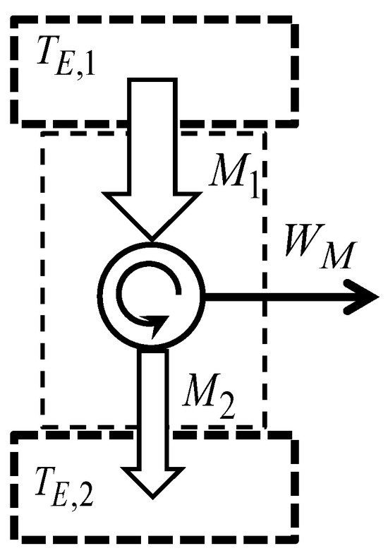
Figure 10.
A schematic representation of the economic engine operating cyclically when in contact with two merchandise reservoirs.
In what follows, [U] is the merchandise transfer interaction with the TE,1 [U/€] merchandise reservoir, [U] is the merchandise transfer interaction with the TE,2 [U/€] merchandise reservoir, and [U] is the merchandise wealth transfer interaction, all of them in one cycle. No merchandise unit accumulation exists in a cycle, for which is [U].
Merchandise unit balance Equation (11) integrated for one cycle time gives
and merchandise economic entropy balance Equation (29) integrated for one cycle time (in the limit economically reversible situation), for which there is no merchandise economic entropy generation, gives
The combination of Equations (74) and (75) allows obtaining that
The economic system operating through the economic reversible cycle receives merchandise M1 [U] from the merchandise reservoir at the higher economic temperature TE,1 [U/€], delivers the merchandise wealth [U], and releases the merchandise [U] to the merchandise reservoir at the lower economic temperature TE,2 [U/€]. The previous period may be rewritten using the unit prices instead of the economic temperatures. The economic system operating through the economic reversible cycle receives merchandise M1 [U] from the merchandise reservoir at the lower unit price p1 [€/U], delivers the merchandise wealth [U], and releases the merchandise [U] to the merchandise reservoir at the higher unit price p2 [€/U]. Dimensionless factor [-] can be referred to as the economic Carnot factor, similar to the dimensionless factor [-] that is referred to as the Carnot factor in Thermodynamics.
The perfect (reversible) economic engine, operating cyclically when in contact with the two merchandise reservoirs at economic temperatures TE,1 [U/€] and TE,2 [U/€], [U/€], is not able to fully convert the merchandise M1 [U] received from the merchandise reservoir at the higher economic temperature TE,1 [U/€] in merchandise wealth, but only the fraction [U], and forcedly releases merchandise [U] to the merchandise reservoir at the lower economic temperature TE,2 [U/€].
The (perfect, reversible) economic Carnot engine, operating through the (economically reversible) economic Carnot cycle, is the one allowing obtaining the maximum merchandise wealth WM,max [U] taking advantage of the M1 [U] merchandise units received from the merchandise reservoir at the higher economic temperature TE,1 [U/€] and of the economic temperature difference [U/€], and from Equations (76) and (77) [U] and [U], or [U] and [U].
In the economic Carnot cycle, merchandise M1 [U] is purchased at the higher economic temperature TE,1 [U/€] (at the lower unit price p1 [€/U]), entering the economic system with the associated merchandise economic entropy [€] (with the associated merchandise financial value [€]). Merchandise [U] leaves the economic system (is sold) at the lower economic temperature TE,2 [U/€] (at the higher unit price p2 [€/U]), with the associated merchandise economic entropy [€] (with the associated merchandise financial value [€]). In the economically reversible process, it suffices to sell the [U] merchandise units at the higher unit price p2 [€/U] to obtain the money necessary to purchase the M1 [U] merchandise units at the lower unit price p1 [€/U], and thus the units of merchandise wealth [U] can be seen as obtained for free, at a null unit price, or at an infinite economic temperature. This is the reason why [U] is merchandise wealth (merchandise with a null unit price). This is why and how the economic Carnot cycle allows obtaining the maximum merchandise wealth from merchandise being traded received (entering the economic system) at the higher economic temperature TE,1 [U/€] (at the lower unit price p1 [€/U]), taking advantage of the economic temperature difference [U/€] (taking advantage of the unit price difference [€/U]).
The normal of economic activity is to create merchandise as wealth and introduce it into the market giving it a unit price in order to generate merchandise economic entropy (to generate merchandise financial value). The economic normal is not to have the economic Carnot engine operating cyclically to obtain the maximum merchandise wealth from merchandise being traded. However, the economic Carnot cycle and the concepts associated with it are of major relevance to the economic Second Law.
It is noted that merchandise being traded can be integrally converted into merchandise wealth in a process, but not in a cycle, the conclusions of this section being highlighted in its title as associated with a cyclic process. This means that it is possible to purchase a given M [U] number of merchandise units at a given unit price, and then to take these WM = M [U] merchandise units as merchandise wealth out of the market, noting, however, that this is not a cyclic process.
A given number of traded merchandise units cannot be integrally converted into the same number of wealth merchandise units, even using the perfect (reversible) economic Carnot engine. In contrast, a given number of wealth merchandise units can be integrally converted into the same number of traded merchandise units. It suffices to take the merchandise wealth WM [U] as merchandise at null unit price (at infinite economic temperature) [U], which is introduced in the market at a finite economic temperature (that is, at a non-zero unit price p > 0 [€/U]). Such an economic process corresponds to the M = NM [U] merchandise units transfer from the infinite economic temperature (from a null unit price) to a finite economic temperature (to a non-zero unit price), since the merchandise units transfer occurs naturally in that decreasing economic temperature direction.
Interestingly, and not less curiously, some of the Carnot notes are on political economics, in the form of 15 postulates; however, they bear no relation to his 1824 pioneering and leading work in Thermodynamics [27]. Those notes, together with his most relevant work on Thermodynamics [27], were published by his brother in 1878 [28], 46 years after his death by cholera at the young age of 36.
5.3. Additional Notes on the Reversible and Irreversible Economic Processes
In a reversible economic process, there is no merchandise economic entropy generation (no merchandise financial value generation), and the process can thus be reversed to restore the initial conditions with no other additional effects. If an economic process is irreversible, it means that some merchandise economic entropy generation exists in such a process, and the economic entropy of the merchandise sold is higher than the economic entropy of the merchandise purchased, thus resulting in some monetary units gain as profit in the process. Once these monetary units are gained, under normal trading conditions, the economic player is not interested in reversing the process, losing the previously gained monetary units as profit.
Let us now analyze the situation of the economic engine (arbitrary in terms of reversibility) operating cyclically when in contact with the merchandise reservoirs at the economic temperatures TE,1 [U/€] and TE,2 [U/€], TE,1 > TE,2 [U/€], as illustrated in Figure 11.
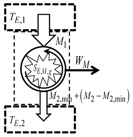
Figure 11.
A schematic representation of the economic engine (arbitrary in terms of reversibility) operating cyclically when in contact with two merchandise reservoirs.
The application of merchandise units balance Equation (11) to the economic system in Figure 11 leads to
As for the economic Carnot cycle [U],
results from Equation (78). The application of merchandise economic entropy balance Equation (29) to the economic system in Figure 11 leads to
As for the economic Carnot cycle [€],
results from Equation (80).
The combination of Equations (79) and (81) allows obtaining that
From the last equation, it is clear how, and why, the economic imperfection (the economic irreversibility, quantified through the merchandise economic entropy generation) lowers the merchandise wealth that could otherwise be obtained through the ideal (perfect, reversible) economic Carnot engine.
The fully irreversible situation analyzed in Section 5.1, for which no merchandise wealth is obtained, conducts to the maximum merchandise economic entropy generation given in Equation (70). The opportunity to obtain merchandise wealth exists, but as this opportunity is not harnessed, merchandise wealth that could otherwise be obtained by taking advantage of the merchandise M1 [U] entering the economic system at the higher economic temperature TE,1 [U/€] and of the economic temperature difference (TE,1 − TE,2) [U/€], TE,1 > TE,2 [U/€] was not obtained, and that opportunity was lost. Multiplying Equation (82) by the lower economic temperature TE,2 [U/€] results in
which gives the lost merchandise wealth (lost in the sense that it could have been obtained but has not been obtained, and not in the sense that it has been obtained and subsequently lost). It is the opportunity to obtain that merchandise wealth that has been lost.
Equation (83) for the irreversible merchandise transfer through the same economic temperature difference (as analyzed in Section 5.1) can be rewritten as
and the financial value generation in the fully irreversible trading process can be seen as the financial value spent to purchase the [U/s] merchandise units at the highest unit price p2 [U/€]. In the reversible economic process, the [U/s] merchandise wealth units are obtained free of charge, without spending any financial value for that. The maximum obtainable merchandise wealth can be retained in the system, or be placed on the market, giving it the maximum unit price p2 [€/U]. In the last case, if it is sold at that unit price, the obtained monetary units can be taken as monetary wealth in the system or used to purchase merchandise units from the market at the lower unit price p1 [€/U]. This is the meaning of economic imperfection, economic irreversibility, and lost wealth in the present context, noting that it is not lost wealth in the sense that it has been obtained and subsequently lost, but in the sense that it is the opportunity to obtain it that has been lost.
5.4. How to Proceed toward More Reversible and Perfect Economic Processes?
More reversible, and thus more perfect, economic processes have lower associated economic entropy generation. Such economic processes require lower financial values to purchase the same number of merchandise units, thus allowing the retention of some available money for free, which can be taken as monetary wealth in the system and be used to purchase additional merchandise units at the lower unit price or to purchase units of other merchandise species. In this sense, the attitude of individuals and corporations guided by decreasing trading, no merchandise unit prices increasing and increased savings of goods and money as wealth, leads to a more reversible, and thus more perfect, economy.
The above statement seems to imply that a dead or frozen economy is the most reversible one, and thus the most perfect one. If we refer to Thermodynamics, the most reversible and perfect engine is an engine with no losses, no imperfections, and no friction. This corresponds to a turned-off, dead, or frozen engine. The engineering challenge is to have the engines operating and producing the expected useful results, but even so, generating as little entropy as possible [3,26]. The same applies to the economic engine and economic activity, which may be live and producing the expected useful results while generating as little economic entropy as possible. Interestingly, this can be achieved by reducing trading operations and the amount of money in the economy, reducing profit from trading, incentivizing direct exchanges of goods and services rather than trading involving long trading chains, increasing direct exchange operations, and avoiding trading operations involving money. Another way is to operate as close as possible to the economic Carnot cycle, minimizing economic entropy generation. Even if the concept of economic irreversibility losses is detailed and clarified using the economic Carnot cycle, the relation between economic irreversibility and economic losses remains also for the non-cyclic processes. In this sense, profit must be avoided, and individuals (fairly) paid for the units of services spent to ensure the economic operations but no more than that (no speculation or deliberate unit price increases). Some initiatives referred to as fair trading, fair cost, and from producer to consumer are guided by these principles of reducing the economic entropy generation. The use of the units of service as labor by the customers, without remuneration, and the reduction of the number of units of services involved in the economic operations, allowing lower unit prices to be paid for the traded merchandise, are other ways to reduce the economic entropy generation, and to contribute to a more perfect and more reversible economy.
6. Interpreting Some Observations of Economic Activity
6.1. Thermodynamics and Economics
The roots of Thermodynamics aim to obtain the maximum mechanical work from thermal engines and reduce the processes’ irreversibility [1,2,3,26]. The reduced irreversibility increases efficiency and competitiveness. Laws and government incentives exist to move towards these increased performance objectives. Economic activity aims, among others, to obtain the maximum profit from both trading and productive and/or creative activities producing new and/or added-value goods and services which, in turn, when sold, lead to increased financial gains. In the economic context, competitiveness is understood in this sense, and Laws and government directives exist to regulate the markets to maintain economic irreversibility (the economic entropy generation, or the financial value generation) within acceptable limits. Market regulations and fair-trade initiatives operate towards reducing the economic entropy generation (reducing the financial value generation).
Thus, Thermodynamics and Economics seem to be on opposite sides, the former trying to minimize the entropy generation and the latter searching for the maximum economic entropy generation. Regulations, Laws, and government initiatives try to contain entropy generation and economic entropy generation within acceptable limits in both cases, yet based on very different reasons: for increased efficiency and performance in the first case, and to curb and contain economic aggressivity in the second case.
From the Thermodynamics viewpoint, entropy generation is a negative thing, meaning imperfection that must be avoided or, at least, minimized [1,2,3,26]; no one is interested in collecting and/or storing entropy, especially generated entropy. From the economic viewpoint, economic entropy generation (the financial value generation) seems to be a positive thing to be explored, driving economic activity. Individuals, corporations, and governments are all interested in generating, collecting, and/or storing economic entropy (merchandise economic entropy and monetary economic entropy).
Entropy generation in thermodynamic processes leads to an increase in the entropy of the Universe. Economic entropy generation leads to an increase in the economic entropy (an increase in the financial value) of a limited part of the Universe, contributing to enriching those controlling and collecting the generated economic entropy.
As the proposed approach demonstrates that the reversible, perfect economy is that with no economic entropy generation, it is, in a way, a thermodynamic-like proof of some of the main claims by E. F. Schumacher in his 1973 book Small is Beautiful [29].
Thermodynamics does not deal with the evaluation of heat transfer and how it is affected by temperature levels or temperature differences and/or other factors, leaving that to the heat transfer disciplines [3]. Similarly, as it is well known, the amount (number of units) of traded merchandise depends, among others, on its unit price, but how the number of merchandise units traded depends on the unit prices is outside the scope of the present work.
6.2. Some Observations and Conclusions on Economic Activity
Observations of economic activity lead to some conclusions which in the economic language seem to be no more than common sense. However, they are somewhat different and allow for different meanings when looking at Economics through the eyes of Thermodynamics; in particular, using the Thermodynamics—Economics parallel approach as proposed in this work, and thus based on physical laws. Among those, the following can be mentioned and highlighted:
- -
- Economic activity is Second Law-oriented: firstly, thoughts are based on the economic Second Law balance equation and its terms, after which actions are taken based on the economic First Law balance equation and its terms to reach the expected (Second Law balance equation) objectives.
- -
- Individuals are naturally trained to conduct economic Second Law balance equation calculations (are naturally trained to conduct financial value calculations), even through quick mental calculations, but not to naturally conduct (thermodynamic) Second Law balance equation calculations.
- -
- Financial accounting of economic processes is based on the economic entropy (financial value) balance equation.
- -
- Trading generates profit but does not add value, corresponding to economic entropy generation (financial value generation) but not to added intrinsic value (not to intrinsic value generation) (economic entropy generation, but no new merchandise units generation).
- -
- Commercial activity increases the unit prices of merchandise (goods and services) but does not increase the intrinsic value of those goods and services.
- -
- Productive and/or creative processes create value (generation of better or new merchandise units), giving rise to added value products and/or services, introduced into the market at higher unit prices, or to new products and/or services generation introduced into the market at finite unit prices.
- -
- Frequently, some goods are obtained (purchased) as merchandise, at given unit prices, but they are used or stored as merchandise wealth (with no trading motivations), and they can later be treated again as merchandise, given unit prices, and traded. As referred to in Section 2.2, for example, the load of a truck (the truck itself having been obtained previously as merchandise) is merchandise (tradable) but not the truck itself; however, in a different context, the truck can itself be the traded merchandise.
- -
- Acquisition of goods (merchandise) and their use or storage as wealth even if they are not wealth (they were not obtained at, nor have they, null unit prices), and their eventual later sale is expected by both individuals and corporations.
- -
- Everyone, individuals and corporations, likes to store (set aside) some goods as wealth, thus implicitly assuming that they are not on the market (they have null unit prices). However, if placed on the market, given them non-zero unit prices, which is usually referred to as selling the family silver, in the sense that merchandise wealth is converted into tradable merchandise.
- -
- Accumulation of generated economic entropy (generated financial value) is expected by both individuals and corporations.
- -
- Accumulation of (merchandise and monetary) wealth is expected by both individuals and corporations.
- -
- Wealth (merchandise and monetary) is not used to satisfy the common day-by-day needs, corresponding to units set aside (not to be traded, nor exchanged in trading).
- -
- Education, training, and skills and competencies acquisition strongly increase the potential for innovation and the creation of new merchandise units. These are originally generated at null unit prices (originally generated as merchandise wealth), but when introduced into the market (giving them non-zero unit prices), that results in merchandise economic entropy generation, that is, in merchandise financial value generation.
- -
- Technologically developed equipment, machines, and facilities strongly increase the potential for high volume flow rate production of new merchandise units as merchandise wealth, which, once introduced into the market (at higher unit prices), results in increased merchandise economic entropy generation, that is, in increased merchandise financial value generation.
- -
- Services that are originally obtained as new units of merchandise wealth at null unit prices and released/sold at non-zero unit prices, and that cannot be later used as tradable merchandise (that are extinguished after their first release, and thus do not have any reproductive effect), are the economic analogs of the mechanical work dissipation into heat by friction. Consider, for example, the cash operator of a supermarket. The cash operator may use its time and skills to perform cash operations for free and thus generate units of service as merchandise wealth. However, as the cash operator is paid for the service, this corresponds to giving unit prices to the so-generated units of service as merchandise wealth and introducing them into the market, which the supermarket customer is paying for. However, the supermarket customer cannot take advantage of the purchased units of service to sell them later at a higher unit price, nor to reproduce/replicate them. The potential of the units of service of the cash operator ceases in the cash operations. The same applies to the cleaning, security, or maintenance services of the supermarket. This corresponds to converting (dissipating) merchandise wealth into tradable merchandise, similar to what happens in Thermodynamics with mechanical work dissipation into heat, which is lost. It is in this sense that those services that cannot be repeatedly traded at higher and higher unit prices, or that do not have a reproductive effect, such as education and training, are like merchandise wealth dissipation as tradable merchandise that is lost, in the sense that it has no further useful effect.
- -
- Non-reproductive services are the economic friction, corresponding to merchandise wealth dissipation, with no further useful economic effect (in the same way as in the thermodynamic systems friction corresponds to mechanical work dissipation as heat, with no further useful effect).
- -
- Reproductive services have some associated economic irreversibility, but they increase the potential for new merchandise units generation, and thus they have further useful economic effects.
- -
- Economic equilibrium (economic reversibility, economic perfection) means trading with no profit, or with new merchandise units generation retention as merchandise wealth.
- -
- Economic irreversibility corresponds to economic non-equilibrium associated with merchandise economic entropy (merchandise financial value) generation, associated in turn with profit generation in trading operations or the introduction into the market (at non-zero unit prices) of the new merchandise units previously obtained/generated as merchandise wealth.
- -
- When central banks introduce monetary values into the economy, they generate monetary economic entropy, which contributes to a greater departure from the economic equilibrium and increased economic irreversibility.
- -
- Natural resources (air, water, solar energy, wind energy, minerals, forests, fuels, etc.) are economic wealth once they can be primarily obtained at null unit prices. However, once harvested and placed on the market, giving them non-zero unit prices corresponds to converting them into tradable merchandise, with the corresponding merchandise economic entropy generation (merchandise financial value generation).
- -
- Individuals and corporations strive to improve their performances in terms of economic growth, which corresponds to the increase in economic entropy through economic entropy generation (economic irreversibility and economic imperfection); they do not strive to move toward economic reversibility and perfection.
- -
- Market regulation and fair-trading initiatives lead to a less aggressive economy, containing economic entropy generation (containing financial value generation), pulling toward a more perfect and more reversible economy.
- -
- Inflation corresponds to an increase in the unit prices of merchandise (goods and services) which is not accompanied by any change, improvement, or intrinsic added value of those goods and services, corresponding thus to merchandise economic entropy generation (requiring increased numbers of monetary units in the purchasing and selling of those merchandises).
- -
- In the past, central banks had the equivalent of the circulating monetary units in gold, which is no longer the case. The financial markets take the monetary units as merchandise, with no effective merchandise counterpart existence. The monetary financial values involved in the financial markets are thus artificial monetary economic entropy, in the sense that they have no effective (real merchandise) counterparts.
- -
- Donations are (merchandise or monetary) wealth transfer interactions, as they are not motivated by trading, and the donated money is not exchanged as compensation for merchandise trading. Donations have associated null unit prices.
- -
- Taxes paid to the state are monetary wealth transfers, as they are not monetary units exchanged as compensation for merchandise trading. In a way, taxes paid to the state can be seen as forced donations to the state, and the money collected by the state is monetary wealth.
- -
- When the state grants a subsidy for purchasing goods or services, it is as if it was providing the purchase of those goods or services at lower unit prices. The state enters monetary wealth (collected from the taxes paid to it) into the process, which is transferred to the merchandise seller (who is selling the merchandise at a higher unit price (at a lower economic temperature)) as monetary exchange involved in the merchandise purchasing, the merchandise becoming available at a lower unit price (at higher economic temperature). It is as if merchandise were transferred from the lower economic temperature to the higher economic temperature and thus in a direction contrary to that of normal merchandise transfer, using the invested wealth for that purpose. This process is similar to a heat pump, which receives mechanical work (heat and infinite temperature) to promote heat transfer from a lower temperature to a higher temperature, thus in a direction contrary to that of normal heat transfer, using the invested mechanical work for that purpose. Thus, a subsidy from the state acts like a merchandise pump, promoting merchandise transfer from a lower economic temperature (a higher unit price) to a higher economic temperature (a lower unit price), thus economically heating the economy.
- -
- If I grow corn and my neighbor grows beans, and I exchange some of my corn for some of his beans, but without me selling him corn and him selling me beans, there are no unit prices for the corn or beans, there is no merchandise traded, and there is no money involved in the process. Only merchandise wealth is generated and transferred in such a process, and no economic entropy (no financial value) is generated. This is thus a perfect, economically reversible, economic process.
- -
- If I invest some of my time and skills, which I have available free of charge (at null unit prices), to clean my house, I do not need money to pay for house cleaning services. In such a process, I am using generated merchandise (services) wealth (time and skills), which is destroyed in the cleaning operation, and neither merchandise to be traded nor money has been involved in such a process, which does thus not contribute to economic entropy generation. Everything we can do for ourselves, using our time, skills, and resources, does not involve the trade of merchandise or the exchange of money and does not contribute to the generation of economic entropy.
7. Finishing Notes
This work develops and sets out a structure for looking at Economics through the eyes of Thermodynamics. Its main conclusions include the fully achieved main objectives itemized at the end of Section 1. Additionally, the structure and the analysis tools developed and introduced facilitate (among others) the following:
- -
- Revisiting, reviewing, comparing, adopting, adapting, and perhaps redefining some of the concepts, viewpoints, and insights of Thermodynamics and Economics;
- -
- A different and new perception of Economics and economic activities from the perspective of Thermodynamics, with a significant potential for discovery and knowledge creation in both Economics and Thermodynamics;
- -
- A set of concepts and quantitative tools for economic interpretations and analyses through the lens of Thermodynamics;
- -
- Opening new ways of thinking and analysis, outside the box, in both Economics and Thermodynamics;
- -
- New analyses, observations, interpretations, methodologies, conclusions, bridges, and interrelations in Economics and Thermodynamics, additionally relating and comparing these two fields;
- -
- Conducting more advanced and specific analyses, using the new tools, from which new and important revelations, relations, insights, and interpretations could emerge in both Economics and Thermodynamics;
- -
- Analysis of economic processes and economic systems from new perspectives and using new tools, derived from physical laws;
- -
- Obtaining the best from the cross-fertilization of Thermodynamics and Economics, with mutual benefits and the development of a fertile interface area with immense potential;
- -
- New pedagogical approaches for both Thermodynamics and Economics teaching and learning, with the more easily understandable aspects of one helping to understand the less easily understandable aspects of the other. In addition, new teaching/learning methodologies could emerge from the similarities between Thermodynamics and Economics, even if caution is always needed when teaching/learning through analogies;
- -
- Seeing Thermodynamics and Engineering Thermodynamics as live and relevant disciplines, claiming new and innovative developments, instead of having the commonly misconceived static, stabilized, frozen, dated, and self-contained character;
- -
- The application of the previous point not only in Thermodynamics and Engineering Thermodynamics, but also in Economics and, additionally, in both Economics and Thermodynamics simultaneously, with special emphasis on their interface area;
- -
- Enlarging the capacity of Thermodynamics for the understanding and analysis of numerous phenomena and processes, the proposed similarities giving scope for more new ways of understanding and analysis than before, even in the very different and far- field of Economics.
As referred to in Section 1, the proposed approach represents tremendous pedagogical and scientific opportunities, opening new routes and proposing new explorations in both Thermodynamics and Economics. Given the way the developments are created, from Engineering Thermodynamics to Economics, it seems that the proposed approach opens more routes in Economics, even though it seems that new pedagogical and scientific routes open in both Economics and Thermodynamics.
Not considered in this work, for the sake of conciseness, are the following:
- -
- A four-Laws structure similar to that of Thermodynamics that can be set for Economics;
- -
- Additional interesting and useful observations to be made concerning the economic Carnot cycle;
- -
- A rigorous and detailed derivation of the economic Second Law that can be similarly conducted, as it is well established for the Second Law of Thermodynamics, leading to the formal definition of the economic temperature and economic entropy;
- -
- Formal developments that can be conducted, leading to the definition of the economic temperature scale;
- -
- Similar structures and developments that can be made to regard Economics through the lens of Thermodynamics, broader than those presented in the present work, which will be the subject of future works.
Funding
This work was supported by the projects UIDB/00481/2020 and UIDP/00481/2020—FCT—Fundação para a Ciência e a Tecnologia; and CENTRO-01-0145-FEDER-022083—Centro Portugal Regional Operational Programme (Centro2020), under the PORTUGAL 2020 Partnership Agreement, through the European Regional Development Fund.
Data Availability Statement
Data are contained within the article.
Conflicts of Interest
The author declares no conflicts of interest.
Nomenclature
| E | Energy |
| F | Monetary exchange rate |
| i | ith merchandise species |
| k | kth monetary species |
| m | Number of monetary units |
| M | Merchandise transfer interaction |
| Merchandise transfer flow rate | |
| N | Number of merchandise reservoirs |
| N | Number of units |
| p | Unit price |
| S | Entropy |
| t | Time |
| T | Temperature |
| V | Value (financial value) |
| W | Wealth transfer interaction |
| Wealth transfer flow rate | |
| Subscripts | |
| E | Economic |
| f | Final |
| F | Financial value |
| g | Generation |
| i | Initial |
| i | ith merchandise species |
| in | Inlet |
| j | jth merchandise reservoir |
| k | kth monetary species |
| lost | Lost |
| m | Monetary |
| M | Merchandise |
| out | Outlet |
| p | Purchasing |
| s | Selling |
| t | Trading operation |
| W | Wealth |
References
- Moran, M.J.; Shapiro, H.N.; Boettner, D.D.; Bailey, M.B. Fundamentals of Engineering Thermodynamics, 8th ed.; Wiley: New York, NY, USA, 2014. [Google Scholar]
- Çengel, Y.A.; Boles, M.A. Thermodynamics—An Engineering Approach, 8th ed.; McGraw-Hill: New York, NY, USA, 2015. [Google Scholar]
- Bejan, A. Advanced Engineering Thermodynamics, 4th ed.; Wiley: Hoboken, NJ, USA, 2016. [Google Scholar]
- Samuelson, P.A.; Nordhaus, W.D. Economics, 19th ed.; McGraw-Hill: New York, NY, USA, 2010. [Google Scholar]
- Krugman, P.; Wells, R. Economics, 4th ed.; Worth Publishers: New York, NY, USA, 2015. [Google Scholar]
- Georgescu-Roegen, N. Energy and Economic Myths—Institutional and Analytical Economic Essays; Pergamon: New York, NY, USA, 1976. [Google Scholar]
- Georgescu-Roegen, N. The Entropy Law and the Economic Process; Harvard University Press: Cambridge, MA, USA, 1979. [Google Scholar]
- Georgescu-Roegen, N. La Décroissance; Entropie, Écologie, Économie; Éditions Sang de la Terre: Paris, France, 2006. [Google Scholar]
- Khalil, E.L. The three Laws of Thermodynamics and the theory of production. J. Econ. Issues 2004, 38, 201–226. [Google Scholar] [CrossRef]
- Ferrari, S. Nicolas Georgescu-Roegen & la Bioéconomie; Éditions le passager clandestin: Lorient, France, 2023. [Google Scholar]
- Burley, P.; Foster, J. (Eds.) Economics and Thermodynamics—New Perspectives on Economic Analysis; Springer Science: New York, NY, USA, 1994. [Google Scholar]
- Schulz, M. Statistical Physics and Economics—Concepts, Tools and Applications; Springer: New York, NY, USA, 2003. [Google Scholar]
- Chen, J. The Physical Foundations of Economics—An Analytical Thermodynamic Theory; World Scientific: Hackensack, NJ, USA, 2005. [Google Scholar]
- Kümmel, R. The Second Law of Economics: Energy, Entropy, and the Origins of Wealth; Springer: New York, NY, USA, 2011. [Google Scholar]
- Ayres, R.U.; Nair, I. Thermodynamics and Economics. Phys. Today 1984, 37, 62–71. [Google Scholar] [CrossRef]
- Ayres, R.U. Eco-thermodynamics: Economics and the Second Law. Ecol. Econ. 1998, 26, 189–209. [Google Scholar] [CrossRef]
- McCauley, J.L. Thermodynamic analogies in economics and finance—Instability of markets. Phys. A 2003, 329, 199–212. [Google Scholar] [CrossRef]
- Saslow, W.M. An economic analogy to thermodynamics. Am. J. Phys. 1999, 67, 1239–1247. [Google Scholar] [CrossRef]
- González, J.V. Thermodynamic laws applied to economic systems. Am. J. Bus. Educ. 2009, 2, 83–86. [Google Scholar]
- Annila, A.; Salthe, S. Economies evolve by energy dispersal. Entropy 2009, 11, 606–633. [Google Scholar] [CrossRef]
- Quevedo, H.; Quevedo, M.N. Statistical thermodynamics of economic systems. J. Thermodyn. 2011, 2011, 676495. [Google Scholar] [CrossRef]
- Belabes, A. What can economists and energy engineers learn from thermo-dynamics beyond the technical aspects? Real-World Econ. Rev. 2019, 88, 130–143. [Google Scholar]
- Rashkovskiy, S.A. Thermodynamics of markets. Phys. A Stat. Mech. Its Appl. 2021, 567, 125699. [Google Scholar] [CrossRef]
- Rashkovskiy, S.A. Economic thermodynamics. Phys. A Stat. Mech. Its Appl. 2021, 582, 126261. [Google Scholar] [CrossRef]
- Roddier, F. De la Thermodynamique à l’Économie; Éditions Parole: Artignosc-sur-Verdon, France, 2018. [Google Scholar]
- Bejan, A. Entropy Generation Minimization: The Method of Thermodynamic Optimization of Finite-Size Systems and Finite-Time Processes; CRC Press: Boca Raton, FL, USA, 1995. [Google Scholar]
- Carnot, S. Réflexions sur la Puissance Motrice du Feu et sur les Machines Propres a Développer cette Puissance; Bachelier: Paris, France, 1824. [Google Scholar]
- Carnot, S. Réflexions sur la Puissance Motrice du Feu et sur les Machines Propres a Développer cette Puissance; Gauthier Villars: Paris, France, 1878. [Google Scholar]
- Schumacher, E.F. Small is Beautiful: A Study of Economics as if People Mattered; Blond & Briggs: London, UK, 1973. [Google Scholar]
Disclaimer/Publisher’s Note: The statements, opinions and data contained in all publications are solely those of the individual author(s) and contributor(s) and not of MDPI and/or the editor(s). MDPI and/or the editor(s) disclaim responsibility for any injury to people or property resulting from any ideas, methods, instructions or products referred to in the content. |
© 2024 by the author. Licensee MDPI, Basel, Switzerland. This article is an open access article distributed under the terms and conditions of the Creative Commons Attribution (CC BY) license (https://creativecommons.org/licenses/by/4.0/).