PrOuD: Probabilistic Outlier Detection Solution for Time-Series Analysis of Real-World Photovoltaic Inverters

Abstract

Anomaly detection methods applied to time series are mostly viewed as black boxes that solely provide a deterministic answer for the detected target. Without a convincing explanation, domain experts can hardly trust the detection results and must conduct further time-series diagnoses in real-world applications. To overcome this challenge, we mathematically analyzed the sources of anomalies and novelties in multivariate time series as well as their relationships from the perspective of Gaussian-distributed non-stationary noise. Furthermore, we proposed mathematical methods to generate artificial time series and synthetic anomalies, with the goal of solving the problem of it being difficult to train and evaluate models for real-world applications due to the lack of sufficient data. In addition, we designed Probabilistic Outlier Detection (PrOuD), which is a general solution to provide interpretable detection results to assist domain experts with time-series analysis. PrOuD can convert the predictive uncertainty of a time-series value from a trained model into the estimated uncertainty of the detected outlier through Monte Carlo estimation. The experimental results obtained on both artificial time series and real-world photovoltaic inverter data demonstrated that the proposed solution can detect emerging anomalies accurately and quickly. The implemented PrOuD demo case shows its potential to make the detection results of existing detection methods more convincing so that domain experts can more efficiently complete their tasks, such as time-series diagnosis and anomalous pattern clustering.

1. Introduction

Generally, we refer to available, normal data as regular data. Outlier detection [1], also interchangeably referred to as novelty detection [2] or anomaly detection [3] in the literature, researches detecting abnormal data points or clusters far from the regular data. Due to the various taxonomies, it is necessary to consider research works focusing on the same topic but under different names. We distinguish these terms in Section 3. These outliers may result from unexpected incidents during the operation of a physical system, such as transitory data loss due to a system reset triggered by power failure, enhanced signal noise due to a change in the working environment, or an abrupt change in consumption behavior (e.g., mall closures) due to a special event (e.g., holidays).

Detection mechanisms are applicable in many real-world application scenarios. For example, in the field of energy planning and management, we can usually establish a digital model as a virtual representation of a sophisticated physical energy system, with the aim being simulation, analysis, prediction, dynamic optimization, etc. Through detection mechanisms in digital models, it is possible to monitor high-dimensional data streams more efficiently in real time. Furthermore, detection models can provide early warnings of potential anomalies to assist experts in analyzing complex data streams. Anomaly detection mechanisms can reduce the risk of physical systems operating under abnormal states for a long time, thus protecting physical systems and extending their life cycle. Moreover, detection mechanisms also play a significant role in renewable energy generation and operation. According to the detection results, operators can flexibly manage power generators to prevent damage caused by extreme weather conditions or an abrupt change in the balance between demand and supply.

While there has been plenty of excellent research on detection methods in the literature, their real-world application encounters challenges. When these outstanding detection algorithms are deployed on real-world datasets, these challenges may affect their performance, which may not be commensurate with their performance on public datasets. We have broadly categorized the challenges we encountered into the following four points:

• Imbalanced anomaly data: Anomalies are rare events. Therefore, in most cases, only limited amounts of labeled anomalous data and patterns are available in real-world datasets. The imbalance problem leads to difficulties in optimizing models and evaluating their performance comprehensively.
• Unknown generative process of anomalies: Without prior knowledge of physical systems, information about the generative process of anomalous patterns, such as generative functions and hyperparameters, is mostly inaccessible. Detection models are thus optimized based solely on existing anomalies, leading to overfitting and difficulty in handling unseen anomaly types.
• Suspicious detection results: Traditional detection methods, such as hypothesis tests based on comparing calculated errors with threshold values, offer deterministic results, i.e., it is either abnormal or not. However, these methods often fall short in convincing experts or aiding in root-cause analysis.
• Expensive annotation: Annotating anomalies in real-world data is consistently a temporally and financially expensive task, particularly when dealing with high-dimensional time-series data from complex physical systems. Expert analysis is essential for extracting critical information about anomalous sources, including their duration, influenced channels, and root causes. The absence of accurate annotations can lead to misclassifying abnormal data as regular, resulting in erroneous assessments.

The contributions of this paper can be summarized as follows:

• We gave precise definitions of outlier, anomaly, novelty, and noise and mathematically analyzed their sources in multivariate time series from the perspective of Gaussian-distributed noise.
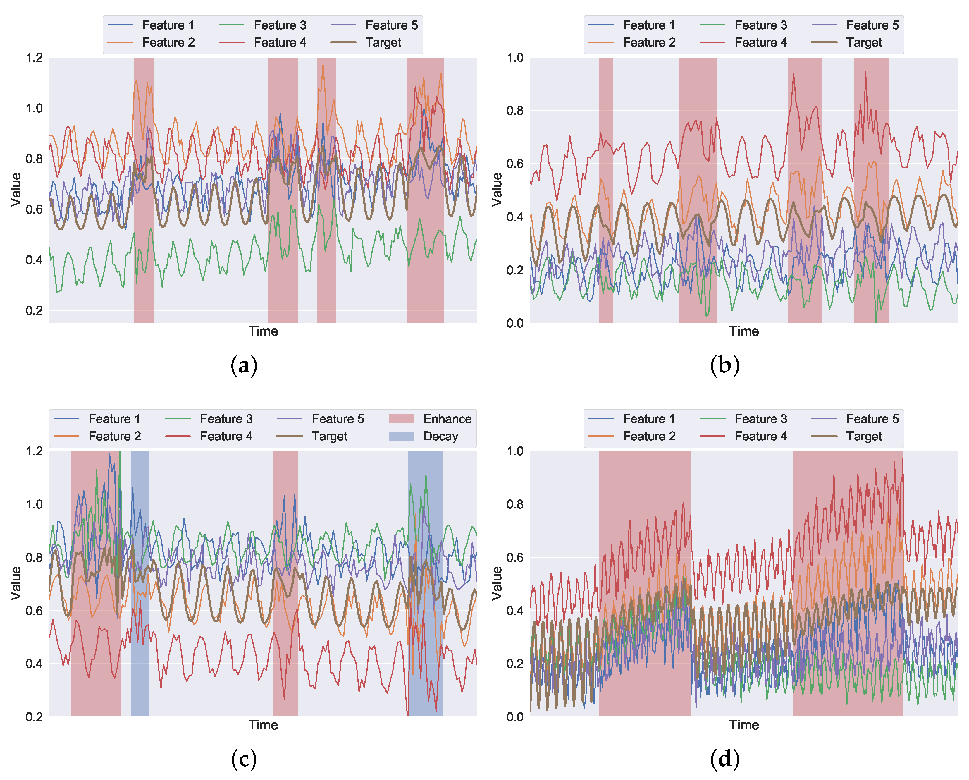
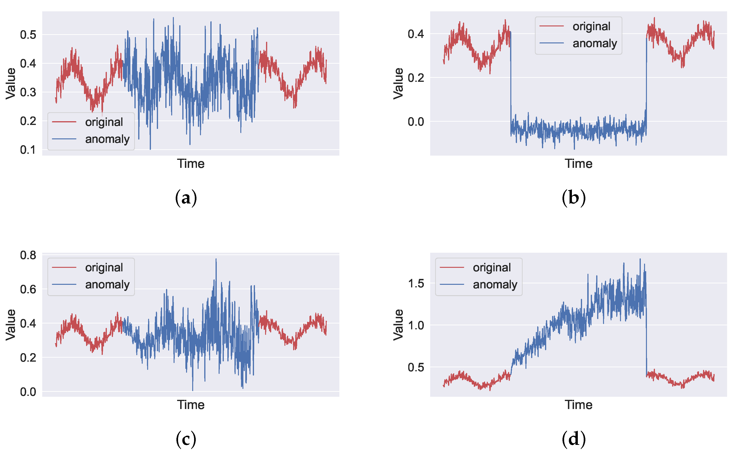
• We proposed generative methods for multivariate artificial time series and four anomalous patterns to address challenges to training and evaluating models when facing an insufficient number of samples.
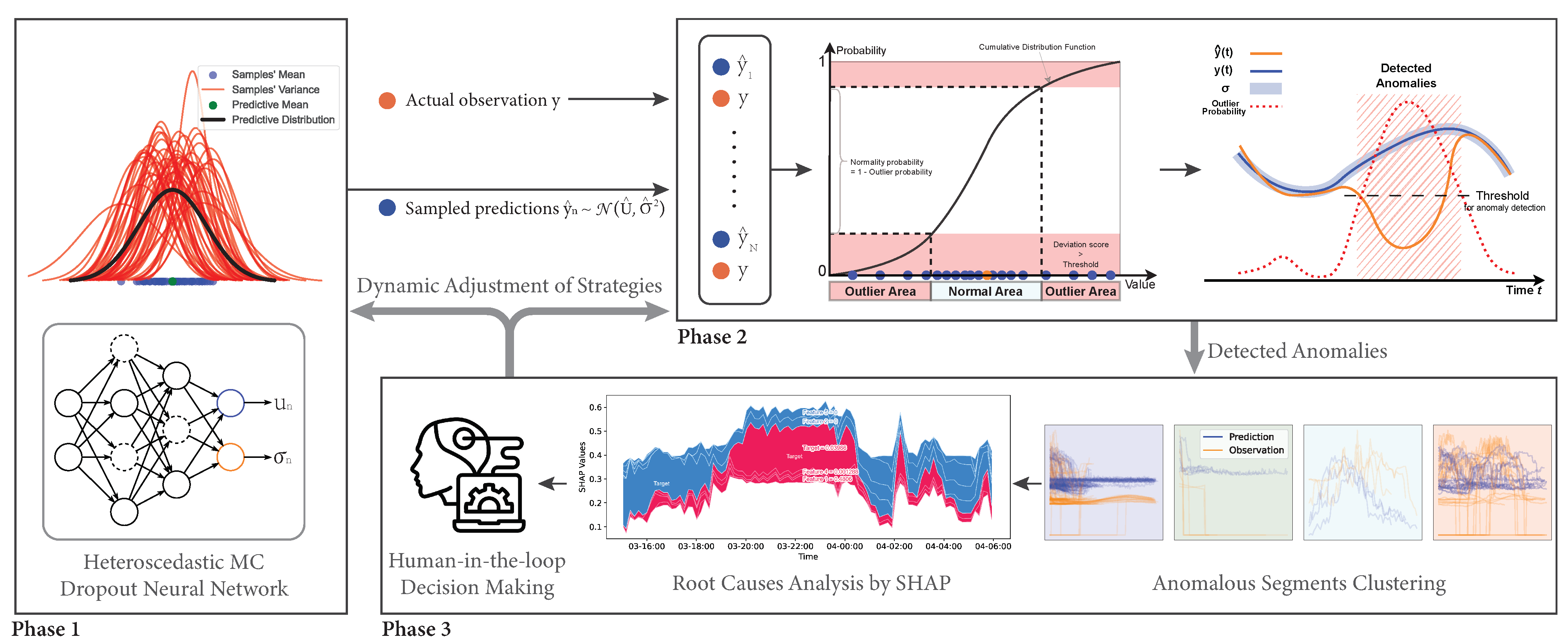
• We proposed the PrOuD solution that describes a general workflow without being restricted to the specific application scenario or the neural network’s architecture. PrOuD is adaptive and can collaborate with various types of Bayesian neural networks. Compared with conventional probabilistic forecasting models and standalone detection models, PrOuD can provide domain experts with enhanced explanations and greater confidence in the detected results through an estimated outlier probability and the use of an explainable artificial intelligence technique. The experimental results on both artificial time series and real-world photovoltaic inverter data demonstrated high precision, fast detection, and interpretability of PrOuD.
• We published the code via (https://github.com/ies-research/probabilistic-outlier-detection-for-time-series (accessed on 5 November 2023)) for interested readers to generate artificial data and reimplement the experiments.

This paper offers specific recommendations and methodologies to readers pursuing various research topics. Contribution 1 can guide researchers working on continual learning algorithms for regression problems [4,5] to define old and new tasks in non-stationary time series. Contribution 2 can help reduce reliance on real-world data collection for training data-driven models, since the synthetic and real-world anomalies show similarities. Additionally, Contributions 3 and 4 propose a human-based interactive machine prototype for monitoring, analyzing, and labeling high-dimensional time series, which will interest readers with an industrial background.

2. Related Work

Compared to supervised learning, unsupervised-learning-based outlier detection methods have less dependence on exact labels about anomalies for training detection models, thus leading to more flexibility in applications. The state-of-the-art unsupervised methods can be briefly divided into two main types [3]: reconstruction-error-based and prediction-error-based. The former utilizes an encoder–decoder architecture to reconstruct inputs at the output layer and then calculate the reconstruction errors, which measure the differences between the reconstructions and the original inputs. The latter assumes the target time series is a (non-)linear combination of multiple input features and attempts to train a model to predict the target. The difference between the predictions and the targets is called the prediction error. Since both types of detection models are trained on regular datasets, when an anomalous perturbation appears in the inputs or the targets, a surprisingly high error can be obtained. The most-recent research works have introduced applying different neural network models to implement detection algorithms. For example, recurrent neural networks (RNNs) were adopted to build encoder-decoder architecture models with the aim of extracting temporal features in latent space for anomaly detection [6,7,8]. The authors of [9,10] proposed unsupervised anomaly detection methods using a convolutional approach coupled to an autoencoder framework. In addition, hybrid methods combining a convolutional neural network (CNN) and long short-term memory (LSTM) have been increasingly proposed, such as [10,11,12,13]. A graph neural network (GNN) considers correlations among sensors and hidden relationships within multivariate time series, and it has also found application in the domain of anomaly detection [14,15,16]. Besides these reconstruction-error-based methods, various neural network models have also been applied to build prediction-error-based detection methods, such as RNNs [17,18,19,20], CNNs [21], and GNNs [22,23]. Most existing anomaly detection methods are typically end-to-end models that predominantly output deterministic anomaly labels: classifying instances as either anomalies or not. However, these deterministic models have limitations in representing the uncertainty associated with their predictions. They lack the capability to indicate the confidence level or the probabilistic nature of their assessments, which is crucial in scenarios for which the distinction between normal and anomalous is not clear-cut. Moreover, the majority of existing research [8,9,13,18] focuses on enhancing the accuracy of detection while often neglecting the importance of providing explanations for the detected results. The authors of [24] introduced a novel design process that integrates human experts into the learning loop by presenting model outcomes in an understandable form. This includes techniques such as model visualization, anomaly visualization, and other interpretable methods, thus facilitating explanations for human experts. However, the work [24] still remains at the conceptual level and has not been implemented. Despite the methods mentioned above achieving remarkable performance in theoretical experiments, the challenges outlined in Section 1 remain unresolved in these works.

3. Artificial Time Series with Synthetic Anomalies

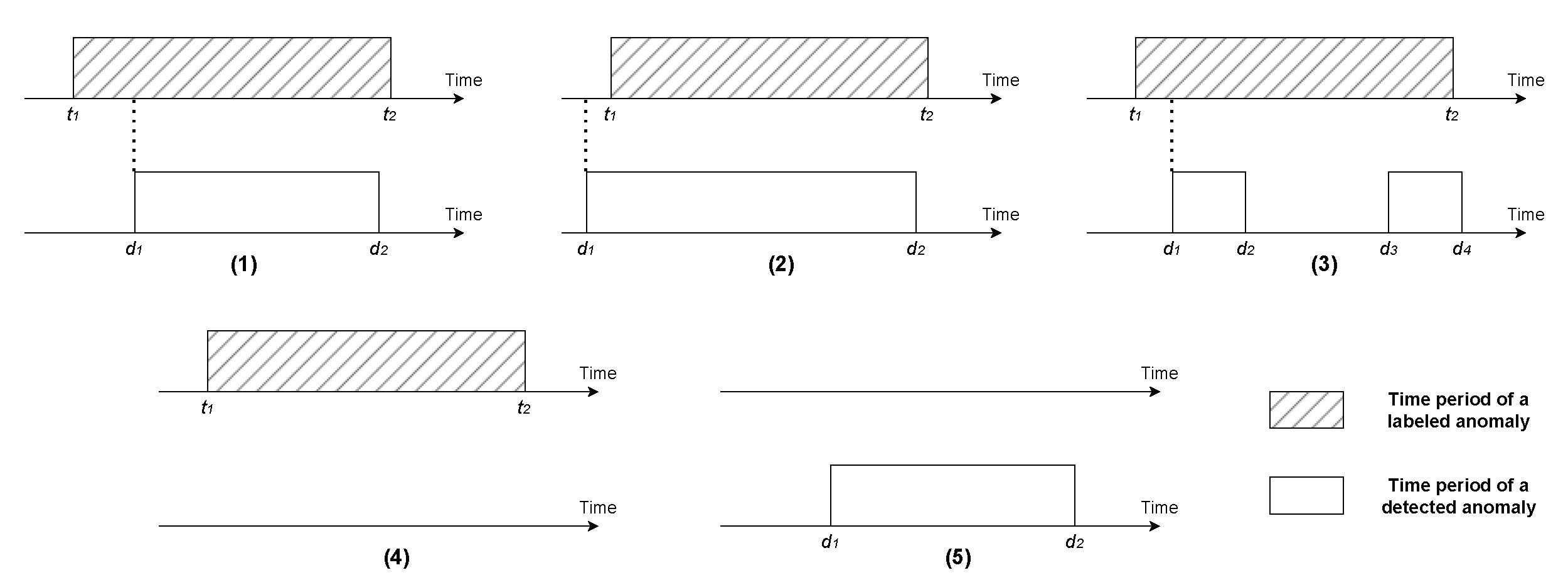
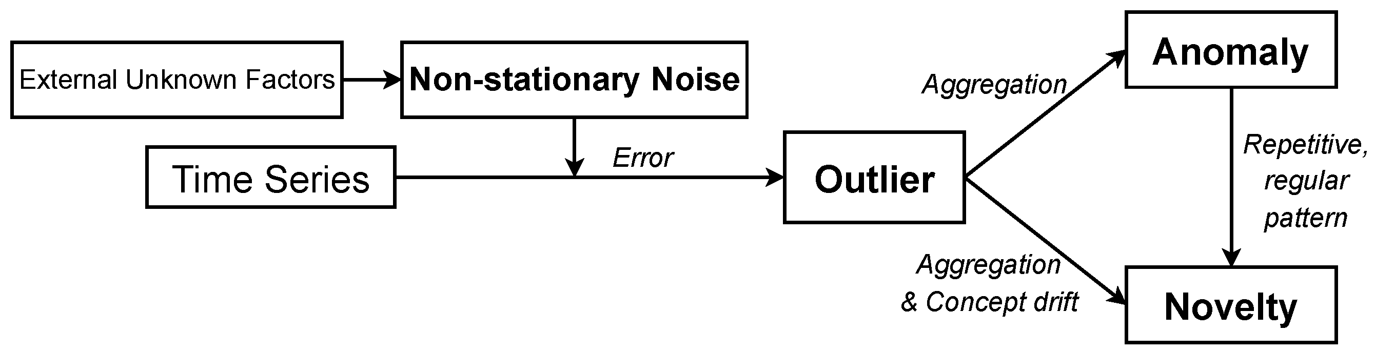
3.1. Terms and Definitions

Assume that a generative function $f\left(·\right)$ describes the underlying generative process of a univariate time series, where the independent variable t indicates the time point. The function $f\left(t\right)$ is a mathematical expression of a complex physical system and is hardly accessible in most cases. What we can observe or measure are the data, referred to as observations. The existence of noise, which is inherent and irreducible, leads to a difference between the outputs of the generative function and the actual observations. According to the available training dataset or prior knowledge of the underlying generative process, we can determine the confidence interval. Outliers are the suspicious observations that are located outside the confidence interval. An uncleaned training dataset containing regular observations and outliers is generally required for training a model.

Outliers can belong to either the underlying generative process or an external event (e.g., changes in the physical system and/or the operation environment, or an unexpected power failure). The former originates from the low-density area of the existing stationary noise distribution; the latter can result from non-stationary noise. Noise is classified by the statistical properties of its distribution. Stationary noise follows a Gaussian distribution with a zero mean and constant variance: ${ϵ}_0\left(t\right)\sim \mathcal{N}\left(0,{\sigma }_0^2\right)$.

By contrast, the mean and/or the variance of non-stationary noise may vary over time. As detailed in

Table 1. Categorization of non-stationary noise.

Non-Stationary Noise $\widetilde{\mathit{ϵ}}\left(\mathit{t}\right)$	Sum of Noise ${\mathit{ϵ}}_0\left(\mathit{t}\right)+\widetilde{\mathit{ϵ}}\left(\mathit{t}\right)$
$$\mathcal{N}\left(\tilde{\mu },{\tilde{\sigma }}^2\right)$$ (1)	$$\mathcal{N}\left(\tilde{\mu },{\sigma }_0^2+{\tilde{\sigma }}^2\right)$$ (2)
$$\mathcal{N}\left(\tilde{\mu }\left(t\right),{\tilde{\sigma }}^2\right)$$ (3)	$$\mathcal{N}\left(\tilde{\mu }\left(t\right),{\sigma }_0^2+{\tilde{\sigma }}^2\right)$$ (4)
$$\mathcal{N}\left(\tilde{\mu },{\tilde{\sigma }}^2\left(t\right)\right)$$ (5)	$$\mathcal{N}\left(\tilde{\mu },{\sigma }_0^2+{\tilde{\sigma }}^2\left(t\right)\right)$$ (6)
$$\mathcal{N}\left(\tilde{\mu }\left(t\right),{\tilde{\sigma }}^2\left(t\right)\right)$$ (7)	$$\mathcal{N}\left(\tilde{\mu }\left(t\right),{\sigma }_0^2+{\tilde{\sigma }}^2\left(t\right)\right)$$ (8)

, the variances of Equations (1) and (3) are constant and are referred to as non-stationary homoscedastic noise, and the variances of Equations (5) and (7) vary over time and are referred to as non-stationary heteroscedastic noise. Furthermore, the means of Equations (1) and (5) are static, whereas the means of the other two are time-dependent. Note that the mean and variance of Equation (1) are static but differ from the ones of ${ϵ}_0\left(t\right)$.

An anomaly consists of a sequence of temporally consecutive outliers from the same pattern and can behave as a gradual or abrupt change. An anomaly is generally caused by an abnormal condition or a fault in the physical system. Anomalies cannot provide any adequate information for maintaining the model’s predictive performance; thus, they should be identified immediately and then removed.

A novelty is also composed of a series of outliers, similar to an anomaly. The main distinction between them is that a detected novelty should be incorporated into the current model through retraining or updating the model since it can provide significant information for improving the performance of the existing model. Distinguishing novelties from anomalies typically requires manual analysis by domain experts with the help of sufficient explanations, which involves consideration of the practical application settings. We think the appearance of novelties is attributed to concept drift. A concept refers to a hypothesis from the space of potential hypotheses that has been found to best fit the given training samples. When the learned concept does not match the newly collected samples, the current model’s performance decreases dramatically. Concept drift is classified as either virtual concept drift or real concept drift [25]. The former results from insufficient knowledge of the input feature space, which causes the learned concept to drift as additional samples are gathered in the application phase. Providing sufficient training samples can help reduce virtual concept drift. The latter refers to the change in the mapping function between the inputs and outputs, which indicates that the physical system learned by the model has been altered, regardless of whether virtual concept drift has occurred or not. For instance, changes in the environment of a wind farm can alter the climatic characteristics surrounding power generators, thus impacting the facility’s electricity generation performance. To maintain prediction performance, the trained model should be retrained using a combination of old and newly collected data. Alternatively, the model can be designed to learn novelties continually in order to accumulate knowledge for handling new tasks [5,24]. A specific case in this context is that a novelty can be composed of a group of anomalies belonging to the same pattern, for which the anomalies appear regularly and repetitively. If the purpose of the application is to detect unexpected observations that do not match the regular data rather than to update the existing model based on newly detected novel data, further distinction between anomalies and novelties does not make much sense. We believe this could explain why detection methods to address similar problems are given different names in most of the academic literature. Figure 1 illustrates the relationships among these terms.

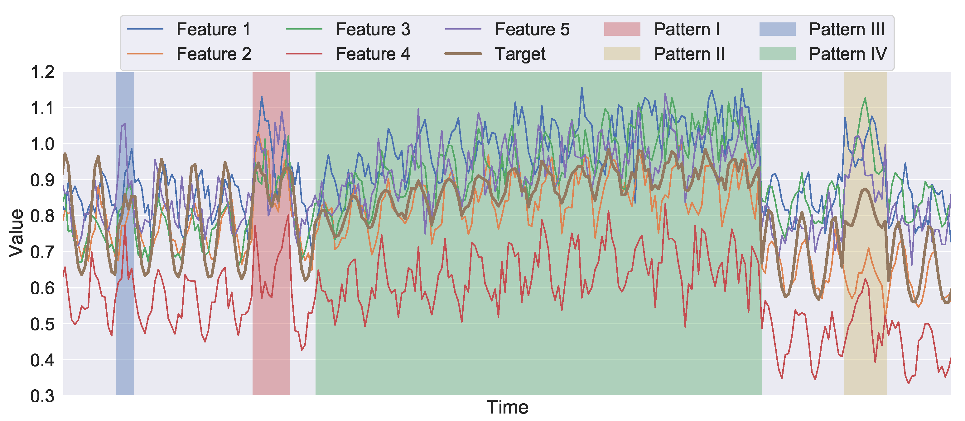
3.2. Artificial Time Series with Synthetic Anomalies

Mathematically, a periodic function repeats its values at specific intervals. It can be defined as $f_T\left(T+t\right)=f_T\left(t\right)$ for all values in the definition domain, where the period T is a constant greater than zero. Considering the periodicity of the time series, the time-dependent generative function of a univariate input is designed as a combination of N periodic functions, i.e., $f\left(t\right)={\sum }_{n=1}^N{A}_n{f}_{T_n}\left(t\right)$, where the amplitude $A_n$, the type of periodic function $f_{T_n}\left(·\right)$ with period $T_n$, and the number of functions N can be customized according to the requirements. In addition, considering the stochasticity, Gaussian noise ${ϵ}_0\left(t\right)$ with a constant variance ${{\sigma }_0}^2$, i.e., ${ϵ}_0\left(t\right)\sim \mathcal{N}\left(0,{{\sigma }_0}^2\right)$, is introduced to the generation. A univariate time series is then generated by combining the generative function and the noise. For example, the j-th dimensional time series of the input space in our experiments is specified as follows:

$$\begin{array}{}\hfill \mathrm{(9)}& x_j\left(t\right)\hfill & =f_{x,j}\left(t\right)+{ϵ}_{x,j}\left(t\right)\hfill \hfill \mathrm{(10)}& \hfill & =A_{d,j}sin\left(\frac{2\pi t}{T_d}+{\varphi }_{d,j}\right)+A_{y,j}sin\left(\frac{2\pi t}{T_y}+{\varphi }_{y,j}\right)+{ϵ}_{x,j}\left(t\right),\hfill \end{array}$$

where $T_d=1440\min$ (i.e., 24 h) and $T_y$ = 525,600 min (i.e., 365 days) refer to the daily period and the yearly period, respectively. In this way, we can generate an input dataset ${\mathbf{X}}^{I\times J}$ containing I samples with J dimensions by customizing the hyperparameters. Next, we define a non-linear generative function $f_y\left(·\right)$ that maps the multivariate input to the univariate output. Selection of the function $f_y\left(·\right)$ can be based on prior knowledge about the physical system. For example, we adopt the third-power of the mean of the input features in our experiments; that is:

$$\begin{array}{}\hfill \mathrm{(11)}& y\left(t\right)\hfill & =f_y\left[{\mathbf{f}}_{\mathbf{x}}\left(t\right)\right]+{ϵ}_y\left(t\right)\hfill \hfill \mathrm{(12)}& \hfill & ={\left[\frac{1}{J}\sum _{j=1}^J{A}_{d,j}sin\left(\frac{2\pi t}{T_d}+{\varphi }_{d,j}\right)+A_{y,j}sin\left(\frac{2\pi t}{T_y}+{\varphi }_{y,j}\right)\right]}^3+{ϵ}_y\left(t\right).\hfill \end{array}$$

Based on the definitions given in Section 3.1, we define an anomalous sequence existing in a univariate time series $x\left(t\right)$ as

$${\mathbf{s}}_{T_a}=\left\{\tilde{x}\left(t\right)=f_x\left(t\right)+{ϵ}_x\left(t\right)+\widetilde{ϵ}\left(t\right)|t_0<t\le t_0+T_a,t\in \mathbb{N}\right\},$$

(13)

with a starting time point $t_0$ and a duration $T_a$. According to the categorization of non-stationary noise, we design the following anomalous patterns to generate various synthetic anomalies in our experiments:

$$\begin{array}{}\hfill \mathrm{(14)}& \hspace{1em} \mathrm{Pattern} \mathrm{I}\text{:}\widetilde{ϵ}\left(t\right)\sim \mathcal{N}\left(\alpha ·f\left(t_0\right),{\beta }^2\right),\hfill \hfill \mathrm{(15)}& \hspace{1em}\mathrm{Pattern} \mathrm{II}\text{:}\widetilde{ϵ}\left(t\right)\sim \mathcal{N}\left(\alpha ·f\left(t\right)+b,{\beta }^2\right),\hfill \hfill \mathrm{(16)}& \mathrm{Pattern} \mathrm{III}\text{:}\widetilde{ϵ}\left(t\right)\sim \mathcal{N}\left(\alpha ·f\left(t_0\right),{\beta }^2·\left(t-t_0\right)\right),\hfill \hfill \mathrm{(17)}& \mathrm{Pattern} \mathrm{IV}\text{:}\widetilde{ϵ}\left(t\right)\sim \mathcal{N}\left(\alpha ·\left(f\left(t_0\right)+\sqrt{t-t_0}\right)+b,{\beta }^2·\left(t-t_0\right)\right).\hfill \end{array}$$

The means of Equations (14) and (16) depend on the value of the time series $f\left(t_0\right)$ at the starting time point $t_0$ of the anomalous sequence. Additionally, the variances of Equations (16) and (17), as well as the mean of Equation (17), are contingent upon the duration of the anomalous sequence.

Various anomalous sequences can be generated by adjusting the hyperparameters $\alpha$, $\beta$, and b, as well as the randomly selected starting point $t_0$. The examples of four anomalous patterns shown in Figure 2 correspond to anomalous phenomena commonly observed in the real world: namely, enhanced noise, downtime, gradually increasing noise, and constant drifting.

Correspondingly, an anomaly in the input space can lead to an anomaly at the output channel within the same period, i.e.,

$$\begin{array}{c}\hfill \tilde{y}\left(t\right)={\left(\frac{1}{J}\left[\sum _{j=1}^J{f}_{x,j}\left(t\right)+\sum _{m=1}^M{\widetilde{ϵ}}_m\left(t\right)\right]\right)}^3+{ϵ}_y\left(t\right),\end{array}$$

(18)

where M denotes the number of affected input channels. Non-stationary noise can also be added solely to the output channels to generate a synthetic anomaly, as expressed in Equation (13).

In this paper, we limited our analysis to univariate time series influenced by a unique anomalous pattern. However, we acknowledge that an anomaly may consist of multiple anomalous sequences from different sources of non-stationary noise and may be temporally correlated in a multivariate time series.

4. PrOuD: Probabilistic Outlier Detection Solution

PrOuD comprises three main phases: probabilistic prediction, detection, and explainable interactive learning, as depicted in Figure 3. PrOuD is designed as a general-purpose workflow with the primary goal of enhancing the limited explainability found in existing methods rather than solely concentrating on improving prediction and classification accuracy. This section, therefore, emphasizes providing a clear description of the input/output and the purpose of each phase. Additionally, it introduces a basic implementation (not state-of-the-art). The inherent customizability of PrOuD suggests that users should adjust the adopted methods and modules according to their specific requirements for practical applications.

4.1. Probabilistic Prediction Phase

The probabilistic prediction phase, referred to as Phase 1 in Figure 3, aims to estimate a predictive distribution with respect to the given multivariate input time-series features. The predictive distribution’s variance indicates the total uncertainty of the model and can be further categorized into aleatoric or epistemic uncertainty [26]. The former stems from inherent randomness and is irreducible. By contrast, the latter is reducible through adequate training samples as it arises due to insufficient knowledge of the optimal model.

Instead of deterministic neural networks optimized by the mean square error (MSE), which neglects the variance and fails to estimate the model’s confidence, we adopt a heteroscedastic deep neural network (HDNN). As shown in Figure 3, its output layer’s dimension is twice the size compared to the dimension of the target. The additional dimension estimates aleatoric uncertainty [27]. HDNN is optimized by the loss function of the negative logarithm likelihood (NLL):

$$\begin{array}{c}\hfill \mathrm{NLL}\left(y\right)=\frac{1}{2{\widehat{\sigma }}_i^2}{∥y_i-{\widehat{\mu }}_i∥}^2+log{\widehat{\sigma }}_i.\end{array}$$

(19)

The output ${\widehat{\mu }}_i$ predicts the mean of the predictive distribution $p\left(y_i\right|$${\mathbf{x}}_i,\mathbf{X},\mathbf{Y})$ and the output ${\widehat{\sigma }}_i$ predicts the corresponding standard deviation.

We can estimate the epistemic uncertainty by treating different neural networks as Monte Carlo samples from the space of all available models, such as deep ensembles [28] or Monte Carlo dropout (MC dropout) [29]. The former employs N neural networks with the same architecture by initializing their weight parameters randomly and training them on shuffled samples of the same training dataset. Dropout is a technique to avoid overfitting by randomly deactivating neurons of the neural network with a fixed probability during training. Subnetworks of the original neural network are created by different neural networks with neurons dropped out. In contrast to regular dropout, MC dropout is also activated at test time. By forwarding the same input through the network while applying dropout N times, N predictions can be obtained. Compared with deep ensembles, MC dropout requires less storage and computation overhead. By combining HDNN with MC dropout or deep ensemble, each network will output a mean ${\widehat{\mu }}_{i,n}$ and a corresponding standard deviation ${\widehat{\sigma }}_{i,n}$ for a given input feature ${\mathbf{x}}_i$. Therefore, the mean and the standard deviation of the overall predictive distribution are

$$\begin{array}{}\hfill \mathrm{(20)}& {\widehat{\mu }}_i\hfill & =\frac{1}{N}\sum _{n=1}^N{\widehat{\mu }}_{i,n},\hfill \hfill \mathrm{(21)}& {\widehat{\sigma }}_i\hfill & =\sqrt{\frac{1}{N}\sum _{n=1}^N\left[{\left({\widehat{\mu }}_{i,n}-{\widehat{\mu }}_i\right)}^2+{{\widehat{\sigma }}_{i,n}}^2\right]},\hfill \end{array}$$

where N denotes the number of neural networks.

Besides reflecting the model’s confidence in the prediction, the estimated predictive distribution can also be applied to determine the threshold for outlier detection using the three-$\sigma$ rule. Moreover, the predictions repetitively sampled from the overall predictive distribution $\mathcal{N}\left({\widehat{\mu }}_i,{\widehat{\sigma }}_i^2\right)$ will be used in the detection phase to estimate the outlier probability of a given observation, which is elaborated on in Section 4.2.

4.2. Detection Phase

The detection phase, denoted as Phase 2 in Figure 3, is designed to estimate the probability of the current actual observation belonging to outliers. This estimation is based on the input of this phase, which includes the overall predictive distribution $\mathcal{N}\left({\widehat{\mu }}_i,{\widehat{\sigma }}_i^2\right)$ from Phase 1 and the given actual observation $y_i$. The estimation can be briefly described as follows. Firstly, for each time point i, we obtain N predictions, ${\widehat{y}}_{i,1},\cdots ,{\widehat{y}}_{i,N}$, by sampling from the obtained predictive distribution about the input time-series features ${\mathbf{x}}_i$. Secondly, we calculate a deviation score to measure the difference between the prediction ${\widehat{y}}_{i,n}$ and the observation $y_i$; this deviation score is used for detection according to a given hypothesis test. Thirdly, we compare each deviation score to a predefined threshold and count the number of deviation scores that are beyond the threshold.

In this paper, we employed the Isolation Forest (iForest) algorithm [30] to compute the deviation scores. The iForest algorithm, an ensemble-based method, operates by isolating outliers in the data rather than profiling normal data points. This is achieved by randomly selecting a feature and then randomly selecting a split value between the maximum and minimum values of the selected feature to partition the data. The process is repeated recursively, and the path length from the root node to the terminating node is used as a measure of normality, where shorter paths indicate potential outliers. The deviation score s at time point i for the n-th sample pair $({\widehat{y}}_{i,n},y_i)$ in an iForest F built by Algorithm 1 is calculated as:

$$s_{i,n}=2^{-\frac{h\left(({\widehat{y}}_{i,n},y_i),F\right)}{c}},$$

(22)

where $h\left(({\widehat{y}}_{i,n},y_i),F\right)$ is the average path length of an instance in F, and c is the normalizing factor. This approach is particularly suited for large-scale datasets due to its linear time complexity and low memory requirement, making it an ideal choice for real-world applications.

Algorithm 1 Isolation Forest Algorithm

1: Input: Dataset $\mathbf{D}$, Number of trees T, Sub-sampling size S 2: Output: Deviation scores for each data point 3: procedure iForest($\mathbf{D},T,S$) 4:     Initialize an empty forest F 5:     for $i=1$ to T do 6:         Sample S points randomly from D to form a sample $D_i$ 7:         $tree\leftarrow$BuildiTree(${\mathbf{D}}_i$) 8:         Add $tree$ to F 9:     end for 10:    return F 11: end procedure 12: procedure BuildiTree($\mathbf{D}$) 13:     if $\left|\mathbf{D}\right|\le 1$ or depth limit reached then 14:         return leaf node with data points from D 15:     else 16:         Select a random feature and a random split value 17:         Split $\mathbf{D}$ into ${\mathbf{D}}_{left}$ and ${\mathbf{D}}_{right}$ based on the split 18:         $leftTree\leftarrow$BuildiTree(${\mathbf{D}}_{left}$) 19:         $rightTree\leftarrow$BuildiTree(${\mathbf{D}}_{right}$) 20:         return node with split feature, split value, $leftTree$, $rightTree$ 21:     end if 22: end procedure

A standard hypothesis test compares the calculation results to a predefined threshold. In this case, threshold selection significantly influences detection accuracy. Considering the existence of extreme outliers, we firstly remove these outliers and then utilize the quantile method for threshold selection. Specifically, we apply the three-$\sigma$ rule, which corresponds to the 99.7% quantile of the deviation score distribution, to set the threshold $\lambda$. The outlier label of the n-th sample pair can be defined by Equation (23), where ‘1’ denotes the outcome as an outlier:

$$l_{i,n}=\left\{\begin{array}{cc}1\hfill & \mathrm{if}{s}_{i,n}>\lambda ,\hfill \\ 0\hfill & \mathrm{if}{s}_{i,n}\le \lambda .\hfill \end{array}\right.$$

(23)

According to the law of large numbers, the outlier probability can be estimated by the ratio of the outlier count to the total prediction count obtained from a large number of samples. The outlier probability $p_i$ at each time step can be calculated according to the following equation:

$$p_i=\frac{1}{N}\sum _{n=1}^N{l}_{i,n}$$

(24)

By estimating the outlier probability, the model’s uncertainty about the time-series prediction is translated into the uncertainty of the detected outlier, rendering the detection results both explainable and convincing.

Time-series data, characterized by their contextual correlation and continuity [31], often present clusters of anomalies that are temporally adjacent and are likely caused by the same underlying anomaly source. To address this, we utilize the Density-Based Spatial Clustering of Applications with Noise (DBSCAN) algorithm [32]. Unlike methods such as sliding windows or K-means, DBSCAN does not require a preset number of clusters and can discover clusters of arbitrary shapes in data with noise. As described in Algorithm 2, DBSCAN works by identifying core points that have a minimum number of neighbors within a given radius and then recursively grouping these core points with their neighbors to form clusters while marking points in low-density areas as outliers. This method is particularly effective for grouping temporally adjacent anomalies and provides more-accurate representation of the underlying anomalous events.

Algorithm 2 DBSCAN Algorithm

1: Input: Dataset $\mathbf{D}$, Epsilon $ϵ$, Minimum points $Mp$ 2: Output: Clusters of data points 3: procedure DBSCAN($\mathbf{D},ϵ,Mp$) 4:     Initialize all points in $\mathbf{D}$ as unvisited 5:     Initialize list of clusters $\mathbf{C}$ 6:     for each point $\mathbf{p}$ in $\mathbf{D}$ do 7:         if $\mathbf{p}$ is unvisited then 8:            Mark P as visited 9:            $NeighborPts\leftarrow$ all points within $ϵ$ distance of $\mathbf{p}$ 10:            if $\mathrm{size}\mathrm{of}NeighborPts<Mp$ then 11:                Mark $\mathbf{p}$ as Noise 12:            else 13:                $\mathrm{Create}NewCluster$ 14:                Add $NewCluster$ to $\mathbf{C}$ 15:            end if 16:         end if 17:     end for 18:     return $\mathbf{C}$ 19: end procedure

We have to emphasize that this study does not aim to compare our approach with the latest or most advanced anomaly detection methods. Instead, our focus is on demonstrating the feasibility and effectiveness of applying anomaly detection techniques to the outputs of probabilistic forecasts. The chosen methods, iForest and DBSCAN, are not exclusive methods capable of achieving this, but they are selected for their suitability for processing and interpreting probabilistic forecast outputs within the context of our specific dataset and anomaly detection challenges.

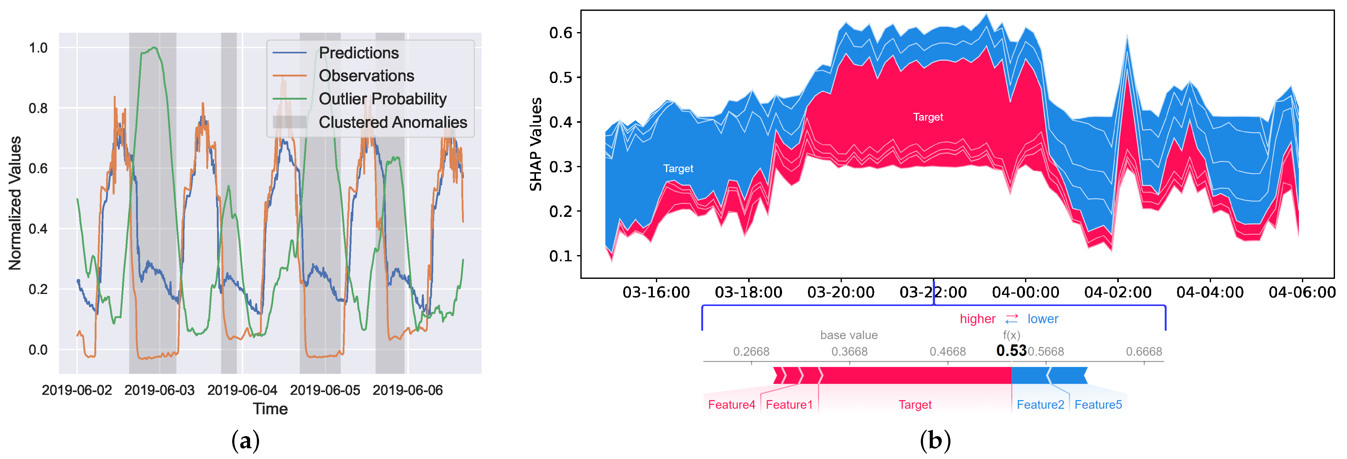
4.3. Explainable Interactive Learning Phase

In the explainable interactive learning phase, referred to as Phase 3 in Figure 3, we try to utilize different techniques to explain the available results (e.g., time-series predictions and detected outliers/anomalies) comprehensively and explicitly. The components inside are customizable and are selected by users according to the concerns and requirements of applications. Here, we introduce two implemented functions as examples, as shown in Figure 3.

One is to find out potential novel patterns by clustering the detected anomalies from Phase 2. As we introduced in Section 3, regularly and recurrently appearing anomalies may be from the same pattern and compose a novelty. Analyzing potential patterns can determine novel tasks that the current model cannot handle and has to learn continually.

The other is to analyze the root sources of detected outliers/anomalies visually using SHapely Additive exPlanations (SHAP) [33], which connects optimal credit allocation with local explanations using the classic Shapely values from game theory. In Phase 2, we obtained multiple anomaly segments. Each contains the J-dimensional input time series and the corresponding target data over the period $T_a$, denoted as ${\mathbf{S}}_{T_a}\in {\mathbb{R}}^{T_a\times (J+1)}$. Vector $\mathbf{j}=\{1,2,\cdots ,J+1\}$ is defined as the set of indices of all channels in ${\mathbf{S}}_{T_a}$. Additionally, we have obtained the corresponding vector of outlier probabilities from Phase 2, denoted as ${\mathbf{p}}_{T_a}=\{p_1,p_2,\cdots ,p_{T_a}\}$. We employ ${\mathbf{S}}_{T_a}$ and ${\mathbf{p}}_{T_a}$ as inputs to the SHAP algorithm to calculate SHAP values for interpreting and visualizing the detection results. SHAP values provide insights into how each univariate time series in the input contributes to the outlier probability $p_i$ for each time step i. This approach aligns with the need for interpretability in complex models, particularly when dealing with time-sensitive and potentially critical data. We use ${\mathbf{S}}_{T_a}$ as the input and ${\mathbf{p}}_{T_a}$ as the target value to fit a tree-based SHAP explainable model denoted as $g(·)$. The variable $g(·)$ is applied to calculate the outlier probability of different channel subsets. The SHAP value ${\varphi }_{i,j}$ for the j-th channel at time step i is given by:

$${\varphi }_{i,j}=\sum _{{\mathbf{s}}_{\mathbf{m}}\left(i\right)\subseteq {\mathbf{s}}_{\mathbf{j}\setminus j}\left(i\right)}\frac{\left|\mathbf{m}\right|!\left(\right(J+1)-|\mathbf{m}|-1)!}{(J+1)!}\left(g\left({\mathbf{s}}_{\mathbf{m}\cup j}\left(i\right)\right)-g\left({\mathbf{s}}_{\mathbf{m}}\left(i\right)\right)\right),$$

(25)

where ${\mathbf{s}}_{\mathbf{j}}\left(i\right)$ denotes the anomaly segment ${\mathbf{s}}_{T_a}$ at time step i, and ${\mathbf{s}}_{\mathbf{m}}\left(i\right)$ denotes a nonempty subset of ${\mathbf{s}}_{\mathbf{j}}\left(i\right)$ excluding the j-th channel, where $\mathbf{m}\subseteq \mathbf{j}\setminus j$. The symbol $\left|m\right|!$ represents the factorial of $\left|m\right|$, and $1<\left|m\right|<J+1$. The probability of the original source for the detected outlier/anomaly is ranked by the quantified contributions of the channels.

Additionally, there are some other promising options to extend the functionalities of Phase 3. For example, we can design a module to evaluate the quality of the predictive uncertainty estimated by the trained probabilistic forecasting neural network under different metrics like Continuous Ranked Probability Score and Calibration Score. The ultimate purpose of Phase 3 is to assist experts with understanding the obtained model and results in a human-understandable way. With this, experts can easily conduct further analysis and make follow-up decisions, such as labeling failure cases, dynamically adjusting the detection strategy, or updating the current prediction model.

In summary,

Table 2. Overview of inputs, operations, and outputs of each phase in PrOuD at the implementation level.

Phase	Inputs	Operations	Outputs
1	Multivariate time series ${\mathbf{x}}_i$	Equations (20) and (21)	Predictive distribution $\mathcal{N}\left({\widehat{\mu }}_i,{\widehat{\sigma }}_i^2\right)$
2	$\mathcal{N}\left({\widehat{\mu }}_i,{\widehat{\sigma }}_i^2\right)$	Equations (22)–(24)	Outlier probability $p_i$ and anomaly segments
3	$p_i$ and anomaly segments	Equation (25) or other explanation methods	Anomaly clusters and visualization results

gives an overview of the inputs, operations, and outputs of each phase in PrOuD.

5. Experiments

This section describes two groups of experiments conducted on artificial time series and real-world solar inverter datasets, respectively. In the experiments, we conducted 24-h-ahead prediction based on the features observed from the previous day with one-hour resolution. The experimental setups are expected to show the adaptability and flexibility of PrOuD by adopting and comparing different networks’ architectures. Additionally, the experimental results from real-world data indicate the existence of the challenges mentioned in Section 1 and display the necessity and significance of explanations for anomaly detection in time series.

5.1. Description of Datasets

The artificial time series is generated with five input features and one output target according to Equations (10)–(12). It consists of 105,120 samples over two years with a resolution of ten minutes. Noise on the input and output channels follows the distribution of ${ϵ}_x\left(t\right)\sim \mathcal{N}\left(0,1\right)$ and ${ϵ}_y\left(t\right)\sim \mathcal{N}\left(0,5\right)$, respectively. The constant amplitudes and phases were randomly selected according to the Gaussian distributions $A_{d,j}\sim \mathcal{N}\left(5,1\right)$, $A_{y,j}\sim \mathcal{N}\left(20,100\right)$, ${\varphi }_{d,j},{\varphi }_{y,j}\sim \mathcal{N}\left(0,1\right)$. The synthetic anomalies were generated according to Equations (14)–(17). We added non-stationary noise solely in the input space, with at least two input channels affected, as defined in Equation (13). A mapped anomaly also appears within the same period, as described by Equation (18). The selection of hyperparameters for generating the anomalies is detailed in

Table 3. Hyperparameters for generating anomalies in the artificial time series. The duration of each anomaly is randomly selected within the given range.

Pattern	Duration	Hyperparameters
I	12–48 h	$\alpha =0.2$, $\beta =0.05$, $b=0$
II	12–48 h	$\alpha =0.2$, $\beta =0.005$, $b=0.005$
III	12–48 h	$\alpha =0.1$, $\beta =0.01$, $b=0$
IV	10–15 days	$\alpha =0.05$, $\beta =0.001$, $b=0$

.

Figure 4 illustrates examples of the synthetic anomalies. Note that an anomaly with gradually decreasing variance is generated if the temporal factor $t-t_0$ in Equation (16) is replaced with $T_a-t$, where $T_a$ refers to the duration of the anomalous sequence.

The real-world photovoltaic inverter data were collected from ten photovoltaic inverters, each with six dependent sensors. The measurement of the insulated-gate bipolar transistor temperature after 24 h was predicted based on historical measurements of five relevant sensors within the previous 24 h. The data for each inverter range from 115 to 210 days, with each inverter having a unique timestamp indicating the start of a labeled failure. The time-series data surrounding the labeled failure were manually divided into a limited number of discrete anomalous sequences, which ranged from one to nineteen for each inverter data series. The percentage of anomalous data over the corresponding inverter data ranges from 1.2% to 10.43%.

Both datasets were normalized to the range of 0 to 1 using Min–Max scaling.

5.2. Experimental Setups

Three probabilistic prediction models were implemented to evaluate PrOuD under different setups. These models are (1) MC dropout heteroscedastic deep neural network (MCDHDNN), (2) voting ensemble of heteroscedastic deep neural network (VEHDNN), and (3) voting ensemble of heteroscedastic long short-term memory (VEHLSTM). The first two models compared MC dropout and voting ensembles for the same architectures of heteroscedastic deep neural networks, while the latter compared different network architectures with the same hyperparameters for deep ensembles.

Under Setup I, five experiments were designed based on the artificial time series, with the first-year data as the training data and the second-year data randomly modified by the generated anomalous sequences for anomaly detection assessment. Each of Experiments I-1, -2, -3, -4 contains the anomalies generated by a single pattern from I to IV. In Experiment I-5, anomalies from the four patterns are mixed, and anomalies from the same pattern are intentionally introduced regularly to the second-year time series for novel pattern clustering, as illustrated in Figure 5. The anomalous samples account for 10% of the whole test data in each experiment.

Under Setup II, each photovoltaic inverter’s data was split into training data (around 43.3% of the data) and test data containing labeled anomalous sequences. The labeled anomalies for the ten inverters’ data comprised, on average, 5.4% of the total data.

5.3. Evaluation Metrics

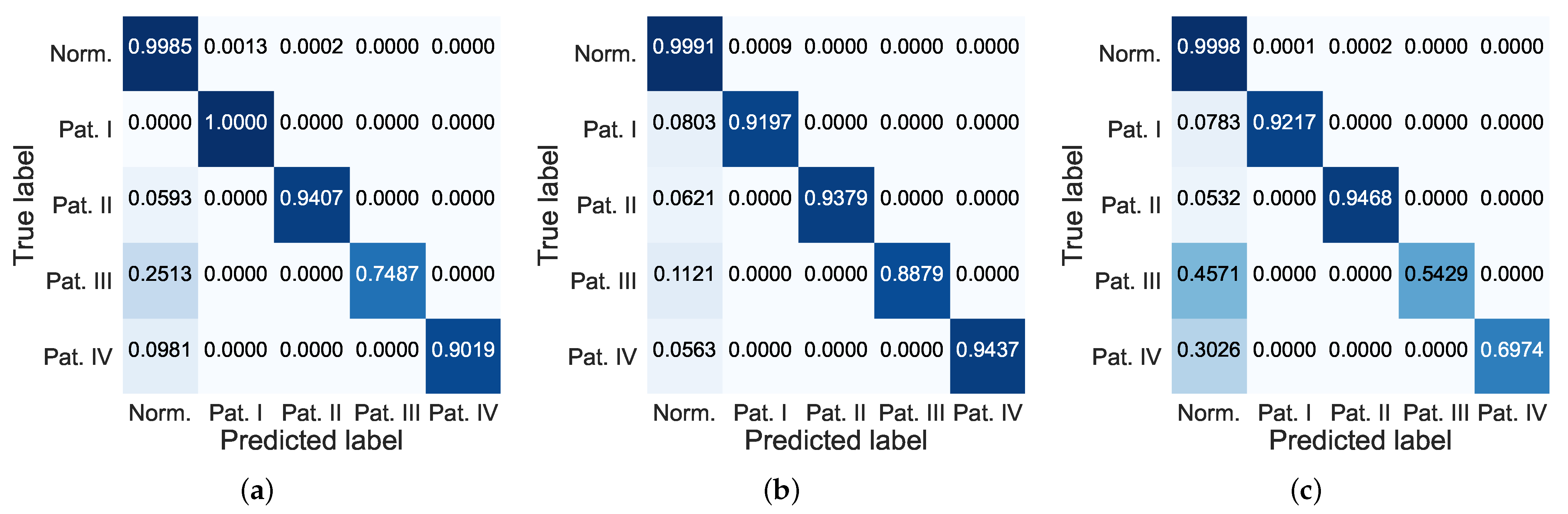
The detection performance of PrOuD incorporating various types of neural networks was assessed using metrics to include Mean Square Error (MSE), precision, recall, F1 score, Area Under receiver operating characteristic Curve (AUC) [34,35], and Mean Time To Detect (MTTD).

MSE is used to evaluate predictive accuracy of the Bayesian neural network in Phase 1 by measuring the average squared difference between the prediction and the actual observation. A lower MSE indicates more-accurate prediction.

$$\mathrm{MSE}=\frac{1}{n}\sum _{i=1}^n{(y_i-{\widehat{y}}_i)}^2$$

(26)

Precision is the ratio of correctly predicted positive observations to the total predicted positives. High precision means the model accurately identifies anomalies with minimal false alarms, leading to efficient resource utilization. Recall is the ratio of correctly predicted positive observations to all observations in the actual class. High recall indicates that the model effectively identifies most anomalies and reduces the risk of undetected fraud. F1 score is the weighted average of precision and recall and is denoted as:

$$\mathrm{F}1\mathrm{Score}=2\times \frac{\mathrm{Precision}\times \mathrm{Recall}}{\mathrm{Precision}+\mathrm{Recall}}$$

(27)

AUC is a comprehensive measure used to evaluate the performance of a binary anomaly detection model. It represents the probability that a randomly chosen positive instance is correctly ranked higher than a randomly chosen negative instance. High AUC indicates that the model has a strong capability to distinguish anomalies from normal observations, which is crucial in scenarios where false positives and false negatives have significant impact.

MTTD measures the interval between the emergence and awareness of an anomaly. The smaller the value, the earlier the detector can identify anomalies. For details, see Appendix A.1.

5.4. Results

Table 4. Experimental results of F1 score, precision, recall, AUC, MTTD (in minutes), and MSE evaluation on the artificial time series in Setup I. MSEs of the three models on the training data are $7.0\times {10}^{-5}$, $5.0\times {10}^{-5}$, and $1.0\times {10}^{-4}$, respectively. Bold numbers indicate the optimal experimental results under the corresponding evaluation metric.

ID	MCDHDNN			VEHDNN			VEHLSTM
	F1 Score	Precision	Recall	F1 Score	Precision	Recall	F1 Score	Precision	Recall
I-1	0.933	0.914	0.953	0.932	0.910	0.954	$\mathbf{0}.\mathbf{936}$	$\mathbf{0.930}$	0.943
I-2	$\mathbf{0.943}$	$\mathbf{0.942}$	0.944	0.927	0.910	$\mathbf{0.946}$	0.925	0.939	0.912
I-3	0.968	$\mathbf{0.978}$	0.958	$\mathbf{0.969}$	0.977	$\mathbf{0.961}$	0.953	0.966	0.941
I-4	0.967	$\mathbf{0.973}$	0.962	$\mathbf{0.974}$	0.967	$\mathbf{0}.\mathbf{982}$	0.891	0.950	0.840
I-5	$\mathbf{0.960}$	0.959	0.962	0.958	0.953	$\mathbf{0.964}$	0.905	$\mathbf{0.991}$	0.832
	AUC	MTTD	${\mathrm{MSE}}_{\mathrm{test}}$	AUC	MTTD	${\mathrm{MSE}}_{\mathrm{test}}$	AUC	MTTD	${\mathrm{MSE}}_{\mathrm{test}}$
I-1	$0.989$	13.5	$1.4\times {10}^{-2}$	$\mathbf{0.990}$	$\mathbf{10.6}$	$1.4\times {10}^{-2}$	0.971	14.2	$\mathbf{1.3}\times {\mathbf{10}}^{-\mathbf{2}}$
I-2	$\mathbf{0.989}$	6.1	$1.8\times {10}^{-2}$	$0.985$	$\mathbf{5.0}$	$2.1\times {10}^{-2}$	0.976	7.1	$\mathbf{1}.\mathbf{5}\times {\mathbf{10}}^{-\mathbf{2}}$
I-3	$\mathbf{0.998}$	27.3	$8.3\times {10}^{-4}$	$0.994$	$\mathbf{24.2}$	$8.3\times {10}^{-4}$	0.980	41.9	$\mathbf{8.1}\times {\mathbf{10}}^{-\mathbf{4}}$
I-4	$0.988$	109.0	$1.9\times {10}^{-3}$	$\mathbf{0.996}$	$\mathbf{90.0}$	$1.8\times {10}^{-3}$	0.932	290.0	$\mathbf{4.3}\times {\mathbf{10}}^{-\mathbf{4}}$
I-5	$0.990$	26.3	$1.1\times {10}^{-3}$	$\mathbf{0.995}$	$\mathbf{24.4}$	$1.1\times {10}^{-3}$	0.972	51.8	$\mathbf{9.2}\times {\mathbf{10}}^{-\mathbf{4}}$

compares the experimental results of the three implementations for Setup I.

By comparing MCDHDNN and VEHDNN, we find that MC dropout helps to gain an advantage in precision, while the voting ensemble outperforms in recall within the same network architecture. The authors of [28] demonstrated that MC dropout can easily give overconfident predictions in comparison to deep ensembles for unseen test samples. Some randomly selected hyperparameters (i.e., $\alpha$, $\beta$, $t_0$) for anomalous pattern configuration may cause only small perturbations in the in-/output channels. We guess that MCDHDNN overlooked these anomalies due to overconfidence, thus leading to relatively lower recall in most experiments. Therefore, as we suggest in Section 4.3, a module in Phase 3 to evaluate the estimated uncertainty may be required in some cases to make experts aware of overconfident predictions. Additionally, we observed higher MTTD values for all models in Experiments I-3, -4, -5. We think this is due to the time-dependent variances of the corresponding patterns, which keep increasing over the duration of the anomaly. As illustrated in Figure 4c,d, the outliers neighboring the start/end of the anomaly are just slightly perturbed. They are easily misclassified as regular observations, thus leading to a delayed detection time. The confusion matrices in Figure 6 show that more outliers of patterns III and IV were misclassified as regular observations.

Surprisingly, VEHLSTM performed poorly in the term of recall in all experiments in Setup I. This outcome can be explained by the better generalization ability of LSTM because the temporal correlation of time series is considered in the architecture of RNN. According to the MSE, VEHLSTM obtained the lowest test error, indicating LSTM can predict unknown data more accurately than the other two models, even though the data are anomalous. However, more-accurate predictions also indicate a smaller prediction error obtained by LSTM, especially when tiny perturbations are added to the input channel. By contrast, we trained MCDHDNN and VEHDNN to slightly overfit on purpose so that they can be more sensitive to abnormal perturbations.

Table 5. Experimental results of F1 score, precision, recall, AUC, MTTD (in minutes), and MSE evaluation on the real-world photovoltaic inverter data in Setup II, presented as mean and variance. Bold numbers indicate the optimal experimental results under the corresponding evaluation metric.

Model	F1 Score	Precision	Recall	AUC	MTTD	${\mathbf{MSE}}_{\mathbf{train}}$	${\mathbf{MSE}}_{\mathbf{test}}$
MCDHDNN	0.700 ($0.168$)	$\mathbf{0.610}$ ($0.197$)	0.902 ($0.042$)	0.974 ($0.024$)	75.1 ($98.0$)	0.002 ($0.0008$)	35.1 ($82.2$)
VEHDNN	$\mathbf{0.705}$ ($0.160$)	0.601 ($0.189$)	$\mathbf{0.903}$ ($0.051$)	0.972 ($0.020$)	$\mathbf{65.6}$ ($79.4$)	$\mathbf{0.001}$ ($0.0005$)	41.1 ($80.7$)
VEHLSTM	0.547 ($0.223$)	0.545 ($0.239$)	0.632 ($0.255$)	0.867 ($0.137$)	183.2 ($281.5$)	0.004 ($0.0018$)	$\mathbf{0.033}$ ($0.016$)

shows the results of Experiment II, which was carried out on the photovoltaic inverter data. MCDHDNN and VEHDNN exhibit similar levels of performance in terms of AUC, recall, and MTTD to those of the experiments in Setup I. Furthermore, we attribute unacceptable precision values to the presence of abnormal samples that are misclassified as normal due to the lack of accurate labels in the dataset, as discussed in Section 1.

Figure 7a shows a fragment of unlabeled photovoltaic inverter data, where the unlabeled anomalies detected by PrOuD are marked with light gray blocks. We can observe that the curve of the outlier probability changes rapidly, indicating its sensitivity to the abnormal data. In addition, our clustering algorithm grouped them into the same anomalous pattern and marked them in the same color. The recurrent anomalies may imply the occurrence of a novelty. In fact, the valley of the observation curve in these blocks is lower than what we observed in the training data. According to our definition given in Section 3.1, the aggregation of these anomalies from the same pattern can form a novelty. The novelty should be incorporated into the current model to extend its knowledge. Unfortunately, even domain experts may not be aware of the existence of a novelty when they label the data. Figure 7b displays the SHAP values of the second anomaly (on the evening of 3 June) in Figure 7a and of an outlier within the same anomaly. The length of each bar corresponds to the quantified score indicating the contribution of the respective channel to the overall outlier probability (0.53 in this case). The red bars indicate channels that increase the outlier probability, while the blue bars indicate channels that decrease this probability. The channel with the longest bar, i.e., the target channel in this case, is the root cause of the outlier according to SHAP. This fits our analysis that a lower valley of the observation curve leads to the anomaly.

6. Conclusions

The application of anomaly detection mechanisms plays a crucial role in supervising energy production and managing energy consumption. In Section 1, we presented potential challenges when applying anomaly detection to real-world time series. The existence of these challenges can significantly affect the performance of excellent detection algorithms. Specifically, the occurrence of rare anomalous data and unknown production processes poses objective difficulties to training and comprehensively evaluating predictive models based on datasets collected from the real world. These challenges can be overcome by collecting more data and annotating as much anomaly data as possible. However, this requires additional investments in time, finances, and human resources for collecting and analyzing anomalies. Moreover, traditional detection methods only provide deterministic results, leading to outcomes that lack sufficient interpretability and credibility. Particularly in the case of handling complex high-dimensional time series, humans are unable to alleviate the workload of time-series analysis through these detection methods.

In order to address the first two challenges, we analyzed multivariate time series and the sources of anomalous data and proposed a straightforward method for generating artificial multivariate datasets with synthetic anomalies in Section 3. Building upon existing techniques, we refined conventional anomaly detection processes and proposed the PrOuD solution. By integrating Bayesian neural networks and Monte Carlo estimation, PrOuD can convert the uncertainty of Bayesian networks regarding time-series prediction into outlier probability estimation, thereby enhancing the credibility of the detection results. In Phase 3 of PrOuD, we illustrated, through two use-cases, how PrOuD utilizes explainable learning and clustering methods to assist experts with time-series analysis and annotation.

In this section, we further present our findings from the experiments, analyze current limitations, and propose ideas for future research expansion.

6.1. Interpretation of Findings

In addition to the real-world photovoltaic inverter dataset, we generated an artificial dataset with the same dimensions. In Setup I, anomalies of single and multiple patterns were incrementally introduced. The goal is to diversify the types of anomalies, increase the quantities, and make reliable anomaly annotation information available in the dataset. Thus, the performance of PrOuD when combining different types of Bayesian networks for various patterns of anomalies can be more comprehensively evaluated.

Upon analyzing the results of Setup I, our findings can be summarized into two points. First, the performance of PrOuD for anomaly detection is correlated with the Bayesian network it incorporates. For example, as mentioned in Section 5.4, due to the overconfidence of MC dropout, the MCDHDNN model achieved higher precision but misses more actual anomalies compared to VEHDNN. Further, VEHLSTM attained lower prediction error on datasets containing anomalies because the temporal correlation of the input time series is taken into account by the architecture of RNN. However, in the unsupervised anomaly detection setting, lower prediction error does not necessarily help us identify anomalies more accurately. This finding actually coincides with our repeated emphasis that PrOuD focuses on increasing the explainability and credibility of detection results rather than on improving the predictive accuracy of the incorporated model.

The second finding is that the diversity of anomalies can impact the model’s performance from different perspectives of evaluation metrics. This finding can be drawn from the results presented in Table 4. In real-world datasets with a limited number of samples, we can hardly observe various types of anomalies simultaneously and determine their sources. Therefore, the analysis of anomaly sources in Section 3 and the proposed customizable generation method can effectively assist with optimizing and evaluating models more comprehensively during the model training phase.

In Setup II, our objective was to illustrate the adverse effects of insufficient annotation information in the dataset on model evaluation rather than evaluate the predictive performance of PrOuD. Our findings was proved by the low precision and relatively high recall presented in Table 5. The absence of annotation information decreases the precision by detecting unlabeled potential anomalies. To further explain our findings, we visualize these detected anomalous time-series fragments in Figure 7. Upon manual analysis, it was observed that the target sensor channel exhibited a different pattern within the temporal range of these anomalies: that is, there were higher valley values. The reason for this change is unknown to us. However, we can see from Figure 7a that the estimated outlier probability curve shows a clear upward trend within each detected anomalous segment, which can greatly enhance the credibility of the detection results. In addition, Figure 7 illustrates how Phase 3 of PrOuD presents the clustering of the detected anomalies (refer to Figure 7a) and provides an explanation for the likely source of the anomalies: namely, the target sensor channel with the largest SHAP value (refer to Figure 7b). This result demonstrates the capability of PrOuD to ease the workload for experts when analyzing high-dimensional time series.

6.2. Limitations and Future Work

This paper addresses the four challenges presented in Section 1 through a systematic analysis and the proposed PrOuD. Considering the diverse topics involved, we have chosen to emphasize a detailed description of each phase in the implementation of PrOuD. By our providing open-source code, PrOuD can be better understood and adapted to fit the needs of specific real-world applications. Hence, in the selection of the prediction model and anomaly detection, our priority was given to features such as less training overhead, consistent output stability, straightforward implementation, and low memory usage. The primary objective was to showcase the PrOuD model’s improvements in credibility and interpretability of anomaly detection results. PrOuD is a flexible framework that can seamlessly incorporate various methods. In future research, the expansion of component selection will involve incorporation with state-of-the-art probabilistic forecasting and anomaly detection methods. Conducting comparative analyses among these models is essential to provide guidance for the practical application of PrOuD in real-world scenarios.

Furthermore, when generating artificial datasets for testing, we make the assumption that each univariate time series is independent of the other inputs and that only one anomalous pattern will occur in a given time period. However, there are complex temporal and/or spatial dependencies between inputs in the real world. Or multiple anomalous patterns may overlap within a given time period. This paper marks the initiation of this research direction and guides our future efforts to analyze and test methods capable of generating diverse anomalous patterns. The aim is to develop a benchmark for testing anomaly detection algorithms in time series.

In Phase 3 of PrOuD, our intention was to illustrate how it aids experts with time-series analysis through the presentation of visual graphs and numerical scores, including outlier probability estimation and SHAP values. Similar to other solutions involving human interaction, a comprehensive assessment of the practical assistance and limitations of PrOuD must be conducted and must rely on actual feedback from experts. Regrettably, we are now facing resource limitations that prevent the execution of such experiments. In future work, we can also research quantifying the results of the assessment and enhancing the interpretability of PrOuD. This aims to ensure its adaptability and effectiveness across various real-world settings.

References

1. Aggarwal, C.C. An introduction to outlier analysis. In Outlier Analysis; Springer: Berlin/Heidelberg, Germany, 2017; pp. 1–34. [Google Scholar]
2. Miljković, D. Review of novelty detection methods. In Proceedings of the The 33rd International Convention MIPRO, Opatija, Croatia, 24–28 May 2010; IEEE: Piscataway, NJ, USA, 2010; pp. 593–598. [Google Scholar]
3. Choi, K.; Yi, J.; Park, C.; Yoon, S. Deep learning for anomaly detection in time-series data: Review, analysis, and guidelines. IEEE Access 2021, 9, 120043–120065. [Google Scholar] [CrossRef]
4. He, Y.; Huang, Z.; Sick, B. Toward Application of Continuous Power Forecasts in a Regional Flexibility Market. In Proceedings of the 2021 International Joint Conference on Neural Networks (IJCNN), Shenzhen, China, 18–22 July 2021; IEEE: Piscataway, NJ, USA, 2021; pp. 1–8. [Google Scholar]
5. He, Y.; Sick, B. CLeaR: An adaptive continual learning framework for regression tasks. AI Perspect. 2021, 3, 2. [Google Scholar] [CrossRef]
6. Tsang, B.T.H.; Schultz, W.C. Deep neural network classifier for variable stars with novelty detection capability. Astrophys. J. Lett. 2019, 877, L14. [Google Scholar] [CrossRef]
7. Su, Y.; Zhao, Y.; Niu, C.; Liu, R.; Sun, W.; Pei, D. Robust anomaly detection for multivariate time series through stochastic recurrent neural network. In Proceedings of the 25th ACM SIGKDD International Conference on Knowledge Discovery & Data Mining, Anchorage, AK, USA, 4–8 August 2019; pp. 2828–2837. [Google Scholar] [CrossRef]
8. Hundman, K.; Constantinou, V.; Laporte, C.; Colwell, I.; Soderstrom, T. Detecting spacecraft anomalies using lstms and nonparametric dynamic thresholding. In Proceedings of the 24th ACM SIGKDD International Conference on Knowledge Discovery & Data Mining, London, UK, 19–23 August 2018; pp. 387–395. [Google Scholar]
9. Thill, M.; Konen, W.; Bäck, T. Time series encodings with temporal convolutional networks. In Proceedings of the Bioinspired Optimization Methods and Their Applications: 9th International Conference, BIOMA 2020, Brussels, Belgium, 19–20 November 2020; Proceedings 9. Springer: Berlin/Heidelberg, Germany, 2020; pp. 161–173. [Google Scholar]
10. Zhang, Y.; Chen, Y.; Wang, J.; Pan, Z. Unsupervised deep anomaly detection for multi-sensor time-series signals. IEEE Trans. Knowl. Data Eng. 2021, 35, 2118–2132. [Google Scholar] [CrossRef]
11. Zhang, C.; Song, D.; Chen, Y.; Feng, X.; Lumezanu, C.; Cheng, W.; Ni, J.; Zong, B.; Chen, H.; Chawla, N.V. A deep neural network for unsupervised anomaly detection and diagnosis in multivariate time series data. In Proceedings of the AAAI conference on Artificial Intelligence, Honolulu, HI, USA, 27 January–1 February 2019; Volume 33, pp. 1409–1416. [Google Scholar] [CrossRef]
12. Del Buono, F.; Calabrese, F.; Baraldi, A.; Paganelli, M.; Guerra, F. Novelty Detection with Autoencoders for System Health Monitoring in Industrial Environments. Appl. Sci. 2022, 12, 4931. [Google Scholar] [CrossRef]
13. Yang, K.; Wang, Y.; Han, X.; Cheng, Y.; Guo, L.; Gong, J. Unsupervised Anomaly Detection for Time Series Data of Spacecraft Using Multi-Task Learning. Appl. Sci. 2022, 12, 6296. [Google Scholar] [CrossRef]
14. Kim, H.; Lee, B.S.; Shin, W.Y.; Lim, S. Graph anomaly detection with graph neural networks: Current status and challenges. IEEE Access 2022, 10, 111820–111829. [Google Scholar] [CrossRef]
15. Wu, Y.; Dai, H.N.; Tang, H. Graph neural networks for anomaly detection in industrial internet of things. IEEE Internet Things J. 2021, 9, 9214–9231. [Google Scholar] [CrossRef]
16. Tang, J.; Li, J.; Gao, Z.; Li, J. Rethinking graph neural networks for anomaly detection. In Proceedings of the International Conference on Machine Learning, PMLR, Baltimore, MD, USA, 17–23 July 2022; pp. 21076–21089. [Google Scholar]
17. Buda, T.S.; Caglayan, B.; Assem, H. Deepad: A generic framework based on deep learning for time series anomaly detection. In Proceedings of the Pacific-Asia Conference on Knowledge Discovery and Data Mining, Melbourne, VIC, Australia, 3–6 June 2018; Springer: Berlin/Heidelberg, Germany, 2018; pp. 577–588. [Google Scholar] [CrossRef]
18. Nguyen, V.Q.; Van Ma, L.; Kim, J.y.; Kim, K.; Kim, J. Applications of anomaly detection using deep learning on time series data. In Proceedings of the 2018 IEEE 16th Intl Conf on Dependable, Autonomic and Secure Computing, 16th Intl Conf on Pervasive Intelligence and Computing, 4th Intl Conf on Big Data Intelligence and Computing and Cyber Science and Technology Congress(DASC/PiCom/DataCom/CyberSciTech), Athens, Greece, 12–15 August 2018; IEEE: Piscataway, NJ, USA, 2018; pp. 393–396. [Google Scholar] [CrossRef]
19. Shen, L.; Li, Z.; Kwok, J. Timeseries Anomaly Detection using Temporal Hierarchical One-Class Network. In Proceedings of the Advances in Neural Information Processing Systems, Vancouver, BC, Canada, 6–12 December 2020; Larochelle, H., Ranzato, M., Hadsell, R., Balcan, M., Lin, H., Eds.; Curran Associates, Inc.: New York, NY, USA, 2020; Volume 33, pp. 13016–13026. [Google Scholar]
20. Mathonsi, T.; Zyl, T.L.V. Multivariate anomaly detection based on prediction intervals constructed using deep learning. Neural Comput. Appl. 2022, 1–15. [Google Scholar] [CrossRef]
21. Munir, M.; Siddiqui, S.A.; Dengel, A.; Ahmed, S. DeepAnT: A Deep Learning Approach for Unsupervised Anomaly Detection in Time Series. IEEE Access 2019, 7, 1991–2005. [Google Scholar] [CrossRef]
22. Deng, A.; Hooi, B. Graph neural network-based anomaly detection in multivariate time series. In Proceedings of the AAAI Conference on Artificial Intelligence, Virtually, 2–9 February 2021; Volume 35, pp. 4027–4035. [Google Scholar] [CrossRef]
23. Chen, Z.; Chen, D.; Zhang, X.; Yuan, Z.; Cheng, X. Learning Graph Structures With Transformer for Multivariate Time-Series Anomaly Detection in IoT. IEEE Internet Things J. 2022, 9, 9179–9189. [Google Scholar] [CrossRef]
24. He, Y.; Huang, Z.; Sick, B. Design of Explainability Module with Experts in the Loop for Visualization and Dynamic Adjustment of Continual Learning. In Proceedings of the Association for the Advancement of Artificial Intelligence (AAAI), Vancouver, BC, Canada, 22 February–1 March 2022. Workshop on Interactive Machine Learning. [Google Scholar]
25. Gama, J.; Žliobaitė, I.; Bifet, A.; Pechenizkiy, M.; Bouchachia, A. A survey on concept drift adaptation. ACM Comput. Surv. (CSUR) 2014, 46, 1–37. [Google Scholar] [CrossRef]
26. Depeweg, S. Modeling Epistemic and Aleatoric Uncertainty with Bayesian Neural Networks and Latent Variables. Ph.D. Thesis, Technische Universität München, Munich, Germany, 2019. [Google Scholar]
27. Abdar, M.; Pourpanah, F.; Hussain, S.; Rezazadegan, D.; Liu, L.; Ghavamzadeh, M.; Fieguth, P.; Cao, X.; Khosravi, A.; Acharya, U.R.; et al. A review of uncertainty quantification in deep learning: Techniques, applications and challenges. Inf. Fusion 2021, 76, 243–297. [Google Scholar] [CrossRef]
28. Lakshminarayanan, B.; Pritzel, A.; Blundell, C. Simple and scalable predictive uncertainty estimation using deep ensembles. Adv. Neural Inf. Process. Syst. 2017, 30, 6405–6416. [Google Scholar]
29. Gal, Y.; Ghahramani, Z. Dropout as a bayesian approximation: Representing model uncertainty in deep learning. In Proceedings of the International Conference on Machine Learning, PMLR, New York, NY, USA, 20–22 June 2016; pp. 1050–1059. [Google Scholar]
30. Liu, F.T.; Ting, K.M.; Zhou, Z.H. Isolation forest. In Proceedings of the 2008 Eighth IEEE International Conference on Data Mining, Pisa, Italy, 15–19 December 2008; IEEE: Piscataway, NJ, USA, 2008; pp. 413–422. [Google Scholar]
31. Zhang, X.; Lin, Q.; Xu, Y.; Qin, S.; Zhang, H.; Qiao, B.; Dang, Y.; Yang, X.; Cheng, Q.; Chintalapati, M.; et al. Cross-dataset Time Series Anomaly Detection for Cloud Systems. In Proceedings of the USENIX Annual Technical Conference, Renton, WA, USA, 10–12 July 2019; pp. 1063–1076. [Google Scholar]
32. Ester, M.; Kriegel, H.P.; Sander, J.; Xu, X. A density-based algorithm for discovering clusters in large spatial databases with noise. In Proceedings of the Second International Conference on Knowledge Discovery and Data Mining, Portland, Oregon, 2–4 August 1996; Volume 96, pp. 226–231. [Google Scholar]
33. Lundberg, S.M.; Lee, S.I. A unified approach to interpreting model predictions. Adv. Neural Inf. Process. Syst. 2017, 30. [Google Scholar]
34. Tan, S.C.; Ting, K.M.; Liu, T.F. Fast anomaly detection for streaming data. In Proceedings of the Twenty-Second International Joint Conference on Artificial Intelligence, Barcelona, Spain, 16–22 July 2011. [Google Scholar]
35. Hand, D.J.; Till, R.J. A simple generalisation of the area under the ROC curve for multiple class classification problems. Mach. Learn. 2001, 45, 171–186. [Google Scholar] [CrossRef]
Figure 1. The relationships among non-stationary noise, outliers, anomalies, and novelties.
Energies 17 00064 g001
Figure 2. Examples of synthetic anomalies generated by the specific anomalous patterns to mimic real-world phenomena. (a) Enhanced noise (Equation (14)). (b) Downtime (Equation (15)). (c) Gradually increasing noise (Equation (16)). (d) Constantly drifting values (Equation (17)).
Energies 17 00064 g002
Figure 3. Illustration of the three main phases of PrOuD solution: (1) probabilistic prediction, (2) detection, and (3) explainable interactive learning.
Energies 17 00064 g003
Figure 4. Visualization of synthetic anomalies added to the artificial time series. (a) Pattern I (see Equation (14)). (b) Pattern II (see Equation (15)). (c) Pattern III (see Equation (16)). (d) Pattern IV (see Equation (17)).
Energies 17 00064 g004
Figure 5. A fragment of the artificial time series with four-pattern anomalies from Experiment I-5.
Energies 17 00064 g005
Figure 6. Confusion matrices of anomalous segment clustering results for Experiment I-5 using (a) MCDHDNN. (b) VEHDNN. (c) VEHLSTM. Darker colors indicate higher performance of the model in the category.
Energies 17 00064 g006
Figure 7. (a) A segment of the photovoltaic inverter data displaying unlabeled anomalies detected by PrOuD and demarcated by light gray blocks, suggesting they may originate from the same pattern. (b) SHAP values of the second anomaly (on the evening of 3 June) in Figure 7a and of one outlier in the anomaly. SHAP suggests the outlier is caused by a change appearing in the target channel.
Energies 17 00064 g007