Article

Application of the Semi-Markov Processes to Model the Enercon E82-2 Preventive Wind Turbine Maintenance System

by
Mirosław Szubartowski
1,
Klaudiusz Migawa
1,
Sylwester Borowski
1,*,
Andrzej Neubauer
2,
Ľubomír Hujo
3 and
Beáta Kopiláková
3
1
Faculty of Mechanical Engineering, Bydgoszcz University of Sciences and Technology, 85-795 Bydgoszcz, Poland
2
Faculty of Mechanical Engineering, Cuiavian University in Włocławek, 87-800 Włocławek, Poland
3
Faculty of Special Technology, Trenčianska Univerzita Alexandra Dubčeka v Trenčíne, 911 50 Trencin, Slovakia
*
Author to whom correspondence should be addressed.
Energies 2024, 17(1), 199; https://doi.org/10.3390/en17010199
Submission received: 30 November 2023 / Revised: 24 December 2023 / Accepted: 28 December 2023 / Published: 29 December 2023
(This article belongs to the Special Issue Advances in Wind Turbine Vibration Modelling and Control)

Abstract

:
The share of wind energy in the energy mix is continuously increasing. However, a very important issue associated with its generation is the high failure rate of wind turbines. This situation particularly concerns large wind turbines, which are expensive and have a lower tolerance for system damage caused by various failures and faults. Vulnerable components include sensors, electronic control units, electrical systems, hydraulic systems, generators, gearboxes, rotor blades, and so on. As a result, significant emphasis is placed on improving the reliability, availability, and productivity of wind turbines. It is extremely important to detect and identify abnormalities as early as possible and predict potential failures and damages and the remaining useful life of components. One way to ensure turbine efficiency is to plan and implement preventive repairs. This work shows a semi-Markov model of a preventive maintenance system based on Enercon E82-2 wind turbines. The system’s performance quality is evaluated based on profit over time and an asymptotic availability coefficient. The developed model establishes formulas describing the efficiency functions and formulates the conditions for the existence of extremes (maxima) of these functions. Computational examples provided at the end of the paper illustrate the obtained research results. A preventive maintenance model is developed that can be applied to wind turbine hazard prevention (determining optimal times for wind turbine preventive maintenance).

1. Introduction

Wind energy is one of the fastest-growing types of renewable energy sources, used as an effective response to social development and global industrial growth in recent decades [1,2,3]. This process is stimulated by the increasing integration of renewable energy sources, including wind turbines, with the power system. The increase in distributed generation in the share of generating sources in the power grid has resulted in many questions about the reliability and assessment of this type of wind farm [4,5,6]. This assessment is necessary to examine the availability of wind farms, impacting energy costs and economic benefits, as well as what is being done to reduce uncertainty in wind power production forecasts [7,8].
Wind turbines must produce electricity under difficult environmental conditions, which can lead to the occurrence of faults, malfunctions, damages, and inoperability. This is particularly true for offshore wind turbines. Maintaining them is also highly costly [9]. As reported by McMillan and Ault [10], the operational costs of offshore wind turbines are twice as high as those of onshore turbines, constituting 20–35% of the total life cycle costs of wind energy conversion systems. Because of this, it is crucial to enhance the reliability, availability, and productivity of wind power plants. The primary solution employed for this purpose is the monitoring of technical conditions and diagnostic identification of faults and damages. This enables the determination of where failures occur and the assessment of their significance, allowing for appropriate actions to be taken. Such an approach facilitates the prevention of further damage, which could give rise to hazardous situations during the operation of wind turbines. In the work by Tchakoua et al. [11], existing techniques for monitoring wind turbines were discussed, and emerging trends were highlighted. Meanwhile, Liu et al. [12] discussed the most frequent types of faults and damages in turbines, while Lau et al. [13] focused on the main failure types of offshore wind turbines. [14,15] addressed fault-tolerant control, prognosis, and resilient control for wind turbine systems. A review of topics associated with fault prognosis and predictive maintenance was presented by Abid et al. [16].
A wind turbine is a complex machine composed of mechanical, hydraulic, and electrical components. The flow of wind through the rotor blades drives their movement and the rotation of the rotor to which they are attached. Depending on the design, further energy conversion may involve an additional gearbox for acceleration. Mechanical energy from the shaft is transformed into electrical current by the generator. Hydraulic systems of the wind turbine are responsible for adjusting the nacelle and rotor blades to change wind speed. Monitoring the condition of the wind turbine allows for verifying its operational parameters to detect early signs of faults and damage. Diagnostics involve detecting, locating, and identifying existing faults and damages. This enables the planning of repair strategies for the system to prevent complete failures.
Ensuring the availability of wind turbines is often closely linked to ensuring an adequate amount of operational time. Consequently, it becomes possible to carry out minimal repairs, which restore the system to its reliability state just before the damage occurs. However, such actions bring the system to an intermediate state between inoperability and “good as new” operability. This state is termed imperfect maintenance. Many authors have discussed various scenarios of imperfect maintenance in their works [17,18].
By implementing appropriate strategies for preventive and corrective actions, it is possible to reduce the system maintenance costs. Activities carried out as part of such strategies include replacing key system elements and determining the frequency of inspections assessing the technical condition. The schedule for these activities is often established by the system designer or manufacturer. During the operational phase, and after the warranty period has ended, this schedule is often adjusted by the user. Typically, they decide on the replacement of worn-out components. Corrective maintenance (CM) actions always require prior diagnosis of the damage and its identification, making them costly and necessitating highly skilled personnel. Repair costs (CM) are generally higher than those of preventive maintenance (PM). Similarly, average repair times exceed average preventive maintenance times. For certain systems, users opt to repair a damaged component without replacing it. This type of repair can be referred to as minimal repair (MR). Minimal repair restores the damaged object to its state prior to the occurrence of the damage. From this standpoint, some replacements can be considered minimal repairs. Based on this reasoning, a variety of practical models for replacements with minimal repair have been proposed in the literature. For this reason, various scenarios of preventive actions are written to reduce repair costs and increase the readiness of technical facilities. Due to their economic importance, maintenance models are becoming increasingly popular in system reliability research.

2. Materials and Methods

The research work focuses on the operation of Enercon E82-2 (MW) wind turbines—specifically the Wicko 10 MW wind farm. Five Enercon E-82 wind turbines constitute the Wicko wind farm studied here. Historical data were collected for analysis and underwent statistical examination. The primary objective of the study was to develop regression models. The average daily energy amount can be determined from the average daily wind speed using these models. The models developed in this study are based on data stored in the SCADA system and are appropriate for the analyzed wind turbine. This usefulness is due to the lack of analysis of other factors, such as terrain roughness, daytime temperature, and other disruptive factors [17,18,19,20], which may depend on the wind farm’s location. To analyze the problem, we developed two linear regression models. We are the first to analyze the impact of average daily wind speed on energy production in individual months for the entire year of 2019. The second model analyzed the impact of average daily wind speed on weekly energy production throughout 2019. The SCADA system in the wind turbines provided the data used to develop the regression models. The actual data obtained included the average speed (m/s) of wind and the average electricity production (kWh) in the period under consideration. Wind speed is measured using a wind turbine sensor [21].
A mathematical model of the operation and maintenance of the Enercon E82-2 wind turbine was developed in this study; the procedure followed is shown in Figure 1. The wind turbines considered are gearless structures with a rated power of 2 MW each. The mathematical model was developed using semi-Markov processes. Data for the individual operational states of the modeled process were obtained from the SCADA system. The data were for five Enercon E82-2 turbines at the Wicko wind farm and were collected in 2019–2020. The obtained and processed source information included the number of individual operational states in the analyzed period, the duration of individual operational states, the amount of energy produced, and related revenues, as well as the costs incurred during downtime, maintenance, and repair of the analyzed wind turbines.

3. Model of Preventive Maintenance System Based on Wind Turbine Age

3.1. States of the Preventive Maintenance System Model

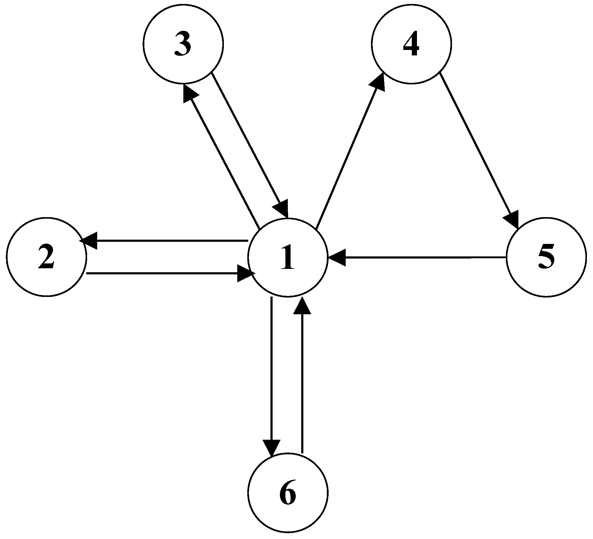
The technical object considered in the study—an Enercon E82-2 turbine—can exist in one of the six states defined in the examined preventive maintenance system model:
  • State 1: Task execution state—electricity production state;
  • State 2: Downtime state caused by lack of access to the power grid;
  • State 3: Downtime state caused by weather conditions;
  • State 4: Waiting state for corrective maintenance after a failure or damage;
  • State 5: Corrective maintenance state after a failure or damage;
  • State 6: Preventive maintenance state—a state in which the operational technical object undergoes preventive maintenance after operating hours and in accordance with the strategy.
Figure 2 is an illustration representing state transitions in the preventive maintenance system model based on the age of the considered technical objects (Enercon E82-2 wind turbines).

3.2. Mathematical Model of the Preventive Maintenance System

To develop a mathematical model, data for five Enercon E82-2 wind turbines were processed. On this basis, average values describing the operation process of an average technical object—a single turbine—were determined. The actual exploitation process was described using a semi-Markovian mathematical model. The main advantage of this type of model is the ability to model the considered process using any type of distribution of random variables, e.g., the Weibull distribution. Additionally, the developed model takes into account the possibility of considering both corrective maintenance after damage occurs and preventive maintenance aimed at preventing damage. However, the limitations are the need for statistical analysis of data and the determination of test results for only a single averaged technical object; in this case, a single wind turbine.
A model was constructed for the illustration shown in Figure 1, assuming that it corresponds to a stochastic process marked X(t). The theory of the semi-Markov processes allowed is described in [22,23,24]. The study considers a 6-state semi-Markov model of preventive maintenance based on age, with state space S = {1 to 6}. If X(t) = i, then at time t, the analyzed object is in state i.
We can determine the Markov chain built into the semi-Markov process when we know the transition probabilities with which the process moves from state to state. In the case of this model, such a transition matrix can be written as:
P = 0 p 12 p 13 p 14 0 p 16 p 21 0 0 0 0 0 p 31 0 0 0 0 0 0 0 0 0 p 45 0 p 51 0 0 0 0 0 p 61 0 0 0 0 0
pij, i, j = 1 to 6—the probability of transitioning from i to j.
The Markov chain has a steady state probability, which is given by the equation:
P T Π = Π 0 p 21 p 31 0 p 51 p 61 p 12 0 0 0 0 0 p 13 0 0 0 0 0 p 14 0 0 0 0 0 0 0 0 p 45 0 0 p 16 0 0 0 0 0 π 1 π 2 π 3 π 4 π 5 π 6 = π 1 π 2 π 3 π 4 π 5 π 6
where:
  • πi, i = 1 to 6—the steady-state probability of the embedded Markov chain.
We can replace the equation shown in matrix (2) with a system of linear Equation (4), but a normalization condition (3) is introduced to obtain a unique solution
i π i = 1
therefore, the system of linear Equation (4) is written as
π 1 + π 2 + π 3 + π 4 + π 5 + π 6 = 1 p 12 π 1 = π 2 p 13 π 1 = π 3 p 14 π 1 = π 4 p 45 π 4 = π 5 p 16 π 1 = π 6

3.3. Steady-State Distribution of the Markov Chain Embedded within Semi-Markov Process X(t)

To solve Equation (4), the results are formulas defining the steady-state probabilities for the Markov chain under study:
π 1 = 1 m 1 π 2 = p 12 m 1 π 3 = p 13 m 1 π 4 = p 14 m 1 π 5 = p 14 p 45 m 1 π 6 = p 16 m 1
where:
m 1 = 1 + p 12 + p 13 + p 14 1 + p 45 + p 16
The technical object undergoes preventive maintenance at age T, or repair when it is damaged, whichever occurs first. The time to preventive maintenance or the object’s technical repair is determined by T1(x). The variable T1(x) is determined as:
T 1 x = T 1 , gdy T 1 < x x , gdy T 1 x
We assume that if the object has not been damaged after time x, it goes into preventive maintenance mode. The transition of states i = 1 to 6 includes preventive maintenance after time x and becomes a new semi-Markov process with the transition probability matrix P(x). Regarding the previously mentioned matrix P, we only change the first row. In this case, P(x) looks like this:
P x = 0 p 12 x p 13 x p 14 x 0 p 16 x p 21 0 0 0 0 0 p 31 0 0 0 0 0 0 0 0 0 p 45 0 p 51 0 0 0 0 0 p 61 0 0 0 0 0
In addition, the steady-state probabilities for the Markov chain were calculated analogously to Formula (5):
π 1 x = 1 m 2 π 2 x = p 12 x m 2 π 3 x = p 13 x m 2 π 4 x = p 14 x m 2 π 5 x = p 14 x p 45 m 2 π 6 x = p 16 x m 2
where:
m 2 = 1 + p 12 x + p 13 x + p 14 x 1 + p 45 + p 16 x

4. Defining the Objective Function

The semi-Markov model in age-based maintenance has been investigated. This model X(t) is based on six states, with a state space S = {1 to 6}. Let zi, i = 1 to 6 denote the unit profit or cost for state i over time. It is assumed that z1 > 0, and zi < 0 for i = 2, 3, 4, 5, 6. We interpret this as a profit for the object in state 1, while there is a cost for the remaining objects (i = 2 to 6).
The objective function describing the cumulative profit or loss over time, similar to that described in [17], for the considered model of the preventive maintenance system is expressed using the formula:
Z = g ( x ) = π 1 x E T 1 ( x ) z 1 + i = 2 6 π i x E T i z i π 1 x E T 1 ( x ) + i = 2 6 π i x E T i Z = g ( x ) = π 1 x E T 1 ( x ) z 1 + π 2 x E T 2 z 2 + π 3 x E T 3 z 3 + π 4 x E T 4 z 4 + π 5 x E T 5 z 5 + π 6 x E T 6 z 6 π 1 x E T 1 ( x ) + π 2 x E T 2 + π 3 x E T 3 + π 4 x E T 4 + π 5 x E T 5 + π 6 x E T 6
where:
ET1(x)—the time spent in state 1, based on [17]
E T 1 x = 0 x d F 1 ( t ) + x P { T 1 x } E T 1 x = 0 x R 1 ( t ) d t
ET2, ET3, ET4, ET5, and ET6—the mean times in states 2–6, respectively.
Additionally, based on [18], it can be written as:
p12(x) = p12 · F12(x)
p13(x) = p13 · F13(x)
p14(x) = p14 · F14(x)
p16(x) = p16 · F16(x) + R1(x)
where:
F1j(x), j = 2, 3, 4, 6—conditional distribution functions of the time in state 1, given that the next state will be state j, defined in [19]:
F i j t = P τ k + 1 τ k < t X τ k + 1 = j , X τ k = i , f o r   i , j = 1 t o 6
R1(x) = 1 − F1(x)—the reliability function of the random variable T1.
To make further considerations easier, we assume that the following equalities are true:
F12(x) = F13(x) = F14(x) = F16(x) = F1(x)
Therefore, we describe function (9) using the following formula:
g ( x ) = E T 1 ( x ) z 1 + p 12 F 1 x E T 2 z 2 + p 13 F 1 x E T 3 z 3 + p 14 F 1 x E T 4 z 4 + E T 5 z 5 + 1 1 p 16 F 1 x E T 6 z 6 E T 1 ( x ) + p 12 F 1 x E T 2 + p 13 F 1 x E T 3 + p 14 F 1 x E T 4 + E T 5 + 1 1 p 16 F 1 x E T 6
after transformation:
g ( x ) = E T 1 ( x ) z 1 + p 12 E T 2 z 2 + p 13 E T 3 z 3 + p 14 E T 4 z 4 + E T 5 z 5 1 p 16 E T 6 z 6 F 1 x + E T 6 z 6 E T 1 ( x ) + p 12 E T 2 + p 13 E T 3 + p 14 E T 4 + E T 5 1 p 16 E T 6 F 1 x + E T 6

4.1. Conditions for the Existence of a Function Maximum: Profit over Time

Parameters of the analyzed semi-Markov model of the preventive system will enable the formulation of the conditions for the existence criterion function extreme (maximum) (9), that is, probability matrix elements of model state changes P = [pij], i, j = 1 to 6, of the average time of staying in ETi model states and unit profits (expenses) generated in zi, i = 1 to 6 state models. The data shown is input into the model. Their values depend on the type of technical objects tested and the adopted maintenance strategy and operating conditions.
We consider the tested system for the parameter values. The established assumptions need to take into consideration actual relationships between parameters typical for the repair of damaged technical objects and for preventive service:
  • Z1: z1 > 0, zi < 0, for i = 2 to 6; meaning that a technical object generates profit while in state 1 (+) and generates expenses while in states 2–6 (−);
  • Z2: z6 < z5; meaning the cost per unit in state 6 (preventive service) is smaller than the cost per unit in state 5 (correction repair);
  • Z3: z2 < z6 < z5; meaning the cost per unit in state 2 (downtime caused by energy shortage) is smaller than the cost per unit in states 6 (preventive service) and 5 (correction repair);
  • Z4: z3 < z6 < z5; meaning the cost per unit in state 3 (caused by weather conditions) is smaller than the unit cost in states 6 (preventive service) and 5 (correction repair);
  • Z5: z4 < z6 < z5; meaning the cost per unit in state 4 (awaiting correction repair) is smaller than the cost per unit in states 6 (preventive service) and 5 (correction repair);
  • Z6: ET4 + ET5 > ET6; meaning that the average downtime caused by damage to the technical object (total of average time of awaiting correction repair and average correction repair time) is longer than the average preventive service time;
  • Z7: ET4 + ET5 > ET2; meaning that the average downtime caused by damage to the technical object (total of average time of awaiting correction repair and average correction repair time) is longer than the average downtime caused by energy shortage;
  • Z8: ET4 + ET5 > ET3; meaning that the average downtime caused by damage to the technical object (total of average time of awaiting correction repair and average correction repair time) is longer than the average downtime caused by weather conditions.
In these assumptions, we do not take into account all the relationships between average times and unit costs; for example, relationships between ET2, ET3, and ET6. For the system under consideration, it is difficult to clearly determine the relationship between average time values. Further into the work, to formulate conditions for criterion function maximum (9), additional conditions were introduced through Formulas (15) and (18)—for situation criterion function means profit over time or Formula (19)—in the case where criterion function means profit availability.
By introducing the numerator and denominator of criterion function (9) in the following way:
L ( x ) = A 1 E T 1 ( x ) + B 1 F 1 x + C 1 M ( x ) = A E T 1 ( x ) + B F 1 x + C
By analogy, function (9) can also be introduced as follows:
g ( x ) = A 1 E T 1 ( x ) + B 1 F 1 x + C 1 A E T 1 ( x ) + B F 1 x + C
where:
A 1 = z 1 B 1 = p 12 E T 2 z 2 + p 13 E T 3 z 3 + p 14 E T 4 z 4 + E T 5 z 5 1 p 16 E T 6 z 6 C 1 = E T 6 z 6 A = 1 B = p 12 E T 2 + p 13 E T 3 + p 14 E T 4 + E T 5 1 p 16 E T 6 C = E T 6
The following coefficients are introduced to elaborate on conditions for the existence of function maximum:
α = A · B1 − A1 · B = B1 − z1 · B
β = A1 · C − A · C1 = z1 · C − C1
γ = B1 · C − B · C1
Coefficients α, β, and γ are necessary to write sufficient conditions for a function to have extremes. Therefore, sufficient conditions are described below to match the α < 0, β > 0, and γ < 0 inequalities.
Having considered the above:
  • coefficient α is defined as:
α = p12 ET2 (z2 − z1) + p13 ET3 (z3 − z1) + p14 [ET4 (z4 − z1) + ET5 (z5 − z1)] + (1 − p16) ET6 (z1 − z6)
  • Inequality α < 0 is equal to inequality:
z 1 > p 12 E T 2 z 2 + p 13 E T 3 z 3 + p 14 E T 4 z 4 + E T 5 z 5 1 p 16 E T 6 z 6 p 12 E T 2 + p 13 E T 3 + p 14 E T 4 + E T 5 1 p 16 E T 6
  • coefficient β is defined as:
β = ET6 (z1 − z6)
With the established Z1 assumption that: β > 0.
  • coefficient γ is defined using the formula:
γ = [p12 ET2 (z2 − z6) + p13 ET3 (z3 − z6) + p14 [ET4 (z4 − z6) + ET5 (z5 − z6)] ET6
Equation γ < 0 is equal to the equation:
z 6 > p 12 E T 2 z 2 + p 13 E T 3 z 3 + p 14 E T 4 z 4 + E T 5 z 5 p 12 E T 2 + p 13 E T 3 + p 14 E T 4 + E T 5
Conclusions 1 and 2 can be written based on equations and inequalities (15), (16), (18) and (19):
Conclusion 1. 
If we consider that the condition described by formula (15) is met—the inequality α < 0 is true.
Conclusion 2. 
If we consider that the condition described by formula (18) is met—the inequality γ < 0 is true.
Here, sufficient conditions for the existence of a criterion function maximum (9) can be formulated for two variants. In the first variant, the subject for consideration is the random variable class of distribution for this variant, assuming the time preceding damage to the T1 technical object is a random variable during the growth function of damage failure rate λ1(t), that is, T1 ∈ IFR (Increasing Failure Rate). Otherwise, the subject of consideration is the random variable class of distribution with the unimodal function of damage failure rate, that is, T1 ∈ MTFR (Mean Time to Failure or Repair). The results of testing the random variable properties of the MTFR class distribution were described in [19].
Conclusion 3. 
If T1 ∈ IFR, λ1(t) is differentiable α < 0, β > 0, γ < 0, β + γ f1(0+) > 0, λ1(∞) α ET1 + β − α < 0, then the value of the function g(x) is maximum.
Proof. 
The criterion function derivative is as follows:
g x = α f 1 x E T 1 x R 1 x F 1 x + β R 1 x + γ f 1 x M 2 x
with M(x) being a denominator of criterion function g(x).
It is known that if the time preceding damage to T1 belongs to the random variable MTFR class of distribution, then equation H(x) = λ1(x) ET1(x) − F1(x) ≥ 0 for x ≥ 0 is true. The random variable MTFR class of distribution has been tested in [9,10]. To the MTFR class belong distributions of life spans with unimodal function of damage failure rate [11,12]. Considering that derivative H′(x) = λ1′(x) ET1(x), if the failure rate λ1′(x) increases, function H(x) increases as well. Random variable class of distribution with non-decreasing function of failure rate (IFR) is included in the MTFR class. The symbol of derivative is the same as the symbol of function:
h x = α λ 1 x E T 1 x F 1 x + β + γ λ 1 x
H(0+) = 0, therefore h(0+) = β + γ f1(0+) > 0. The fact that α < 0, β > 0, γ < 0, as well as H(x) increase indicates that function h(x) decreases from a value of h(0+) = β + γ f1(0+) > 0 to a value of h(∞) = λ1(∞) α ET1 + β − α < 0. Therefore, the derivative g′(x) changes the symbol from “+” to “–” exactly once, thus, it is concluded that the value of the function g(x) is maximum. □
If λ1(∞) = ∞, then in order to reach the maximum of criterion function g(x), only the following conditions are required: T1 ∈ IFR, differentiability λ1(t), α < 0, β > 0, γ < 0, β + γ f1(0+) > 0. A special example of random variable distribution is the Weibull distribution with the increasing function of failure rate.
Conclusions 1, 2, and 3 indicate that the following condition is sufficient for the existence of criterion function maximum g(x)—profit over time.
Conclusion 4. 
If T1 ∈ IFR, λ1(t) is differentiable, α < 0, β > 0, γ < 0, β + γ f1(0+) > 0, λ1(∞) α ET1 + β − α < 0, the value of function g(x) is maximum.

4.2. Conditions for the Existence of Criterion Function Maximum: Availability

Sufficient conditions for the existence of an asymptotic maximum availability coefficient are formulated below. To get the availability coefficient from the criterion function g(x), the following conditions need to be assumed: z1 = 1, zi = 0, for i = 2 to 6. After taking into account conditions from (9), formula A1 = 1, B1 = 0, C1 = 0 is obtained. Therefore:
α = − B = − p12 ET2 + p13 ET3 + p14 (ET4 + ET5) − (1 − p16) ET6,
β = C = ET6; β > 0,
γ = 0,
Equation α < 0 is equal to equation
E T 6 < p 12 E T 2 + p 13 E T 3 + p 14 E T 4 + E T 5 1 p 16
Taking into account the fact that β > 0 i γ = 0, a condition for the existence of criterion function maximum can be formulated.
Conclusion 5. 
If T1 ∈ IFR, λ1(t) is differentiable, λ1(∞) α ET1 + β − α < 0, and the inequality (20) is fulfilled, then the availability coefficient reaches exactly one maximal value.
Proof. 
In the case of the availability coefficient, the criterion function derivative is as follows:
g x = α f 1 x E T 1 x R 1 x F 1 x + β R 1 x M 2 x
with M(x) being a denominator of function g(x).
If the failure rate λ1(t) increases, then H(x) increases. The derivative has the same sign as the function.
h x = α λ 1 x E T 1 x F 1 x + β
It is known that H(0+) = 0, hence h(0+) = β > 0. The fact that condition (20) is fulfilled indicates that α < 0 and function h(x) is increased from h(0+) = β > 0 to h(∞). If h(∞) = λ1(∞) α ET1 + β − α < 0, then the derivative g′(x) changes the symbol from “+” to “–” exactly once. Therefore, it should be summarized that function g(x) has only one extremum—the maximum. □
Conclusion 5 indicates the following sufficient condition for the existence of criterion function maximum g(x): availability.
Conclusion 6. 
If λ1(∞) = ∞, then in order to reach the maximum of criterion function g(x), only the following conditions are required: T1 ∈ IFR, as well as the condition in formula (20).

5. Calculations Confirming the Model

Example 1. 
In Figure 3, criterion function g(x) graphs have been introduced in the case representing profit over time; however, in Figure 4, if g(x) means availability of the considered technical objects—Enercon E82-2-type wind turbines—Calculations were undertaken using the data.
  • probability matrix values of model P state changes:
P = 0 0.3 0.38 0.21 0 0.11 1 0 0 0 0 0 1 0 0 0 0 0 0 0 0 0 1 0 1 0 0 0 0 0 1 0 0 0 0 0
  • average time of the technical object in a model state in (day): ET2 = 0.11, ET3 = 0.17, ET4 = 0.48, ET5 = 0.44, ET6 = 0.21; for task completion time (useful life) for T1, the Weibull distribution has been adopted, for which the parameter scale value = 8. Four scenarios were studied, where the shape parameter value of the Weibull distribution is ∈{6.5, 8, 9.5, 11};
  • average profit (cost) values per time unit in particular model states in (1k PLN/day): z1 = 4.1, z2 = −2.6, z3 = −2.6, z4 = −2.6, z5 = −17.3, z6 = −7.1.
In both cases where function g(x) means profit over time (Figure 3) and function g(x) means availability (Figure 4), the values of the criterion function take the maximum. In each of the four studied scenarios, for each particular shape parameter value of the Weibull distribution, the time value of preventive service xmax (day) is optimal for what the criterion function g(x) value takes the maximum. Based on the analysis of the given charts, it can be concluded that for an increased shape parameter, the maximum profit increases over time, while at the same time, the xmax value decreases. In the case of availability, along with the increase in the shape parameter value, the maximal value of the function increased while the xmax value remained practically constant at 6 days. Based on the results obtained for the unit profit and the readiness of the analyzed wind turbines presented in Figure 4 and Figure 5, it can be concluded that the average monthly profit calculated is approximately PLN 107–108 000, while the average annual profit is approximately PLN 1,310 000.
Example 2. 
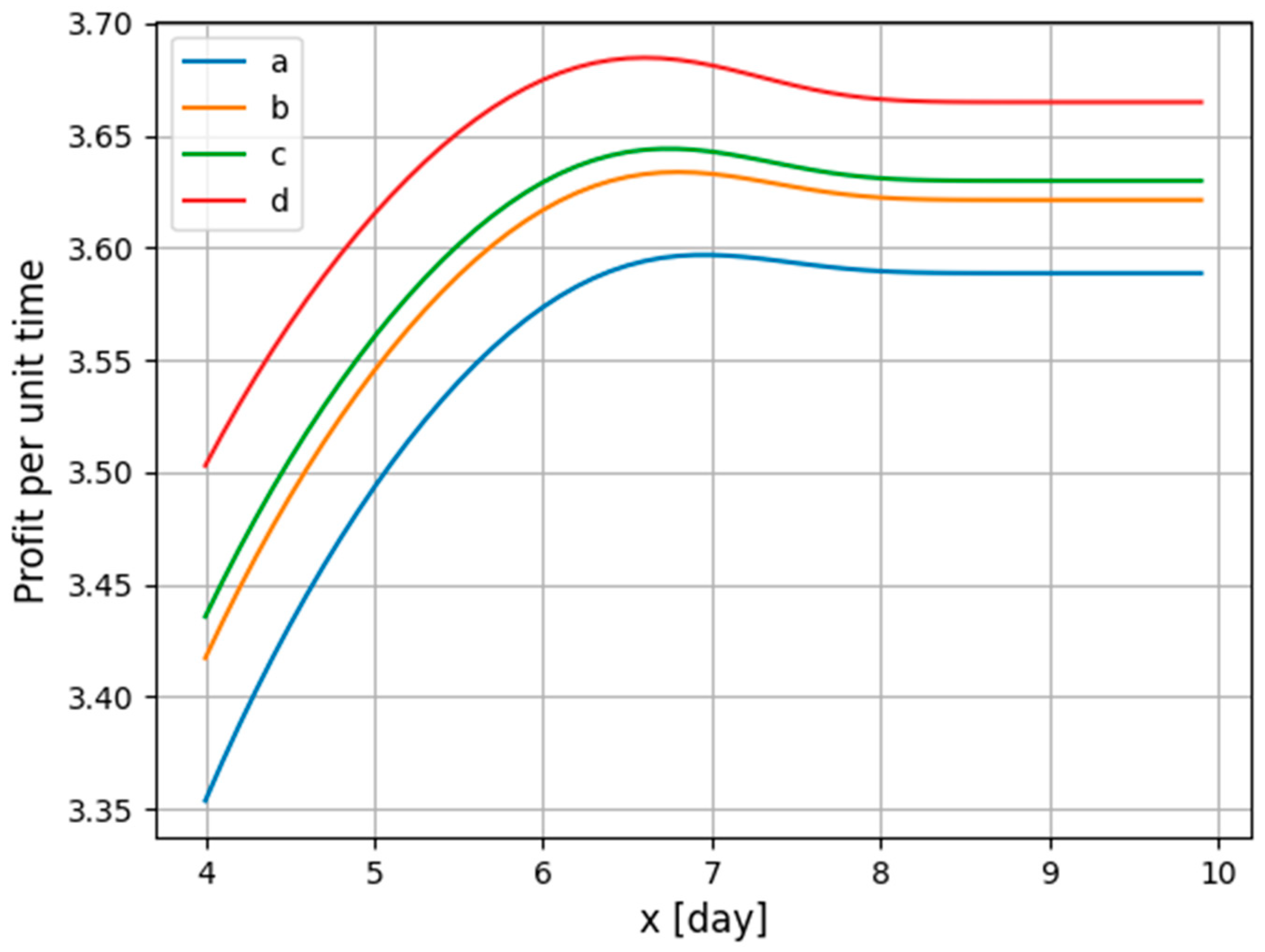
Figure 5 and Figure 6 introduce, respectively, graphs of function g(x) (with g(x) as profit over time and availability of Enercon E82-2-type wind turbines. The calculations were performed using data from example 1, assuming that the task completion time (useful life) T1 based on the Weibull distribution parameters scale value = 7 and the shape value = 10. The graphs introduce four scenarios: scenario a, if the frequency of preventive maintenance is identical to that in example 1; and scenarios b, c, and d if the frequency of preventive maintenance is increased by 15%, 25%, and 35%, respectively, of scenario a.
Based on analysis of the graphs introduced in Figure 5 and Figure 6, it can be noted that with the increase in preventive service frequency, there is an increase in criterion function g(x) for both profit over time and availability; the maximum of function g(x) is achieved for decreasing values of xmax (optimal value of the period preceding preventive service). Increasing the frequency of preventive maintenance for the considered cases results in an increase in the average monthly profit of the wind farm in question by approximately PLN 12.6–15.3 000, and the average annual profit by approximately PLN 151.5–184.3 000.
Example 3. 
Figure 7 and Figure 8 introduce function g(x) graphs (with g(x) as profit and availability of Enercon E82-2-type wind turbine, respectively). The graphs introduce four scenarios: scenario a, for the same data as scenario a in example 2, and scenarios b, c, and d, for which the abilities of production and electric energy storing in state 2 of system modeling are estimated at 50% (line b) and 100% (line c).
Based on the analysis of the graphs introduced in Figure 7 and Figure 8, it can be noted that with the increase in preventive service frequency, there is an increase in criterion function g(x) for availability and profit over time. The maximal value of function g(x) when there is a profit over time unit (Figure 7) is reached for bigger values of xmax (time preceding preventive service), while in the case of wind turbines (Figure 8), it is reached for bigger values of xmax. The development of the possibility of storing electricity in state 2 of the modeled system in 50% (curve b) and 100% (curve c) results in an increase in the average monthly profit of the wind farm in question by approximately PLN 14.5–17.2 000, and the average annual profit by approximately PLN 173.3–PLN 206.2 000.

6. Conclusions

This study introduces the Enercon E82-2 (MW)-type wind turbine preventive service system model, elaborated using semi-Markov processes. Criterion functions are taken into account for the infinite time frame in the elaborated model. Within the introduced model, designating the solution is based on the maximal value of the analyzed functions—profit over time or availability. The conducted analysis provided the basis for describing the necessary conditions for creation function maxima when the time preceding the damage to the wind turbine is a random variable that increases the failure rate. We made assumptions and described the defining conditions needed to describe the relationships between the model’s input parameters and to assess the usefulness of selected input data used to calculate the extremum of the tested criterion functions. The created preventive service system model can be used to designate optimal preventive service strategies in wind turbine exploitation systems (designating optimal times for preventive service of wind turbines). The introduced study results are another stage of work on technical object exploitation system modeling in which preventive replacement is conducted based on age. In the next stages, we plan to introduce a two-criterion model in which choosing optimal (suboptimal) solutions would be realized with the use of the Pareto front as well as genetic algorithms.

Author Contributions

Conceptualization, S.B.; methodology, K.M. and M.S.; software, A.N.; validation, S.B.; formal analysis, A.N.; investigation, M.S.; writing—original draft preparation, S.B. and K.M.; writing—review and editing, Ľ.H. and K.M.; visualization, Ľ.H. and B.K. All authors have read and agreed to the published version of the manuscript.

Funding

This research was funded by Biogazownia Rypin Sp. z o.o. ul. Starorypin Prywatny 51, 87-500 Rypin, and The APC was funded by the Faculty of Mechanical Engineering, Bydgoszcz University of Sciences and Technology.

Data Availability Statement

The data presented in this study are available on request from the corresponding author. The data are not publicly available due to the confidentiality clause in the cooperation agreement with the owner of the Wicko wind farm.

Conflicts of Interest

The authors declare no conflicts of interest.

Abbreviations

CMcorrective maintenance
ET(x)the time spent in state
Fj(x)conditional distribution functions of the time in state
IFRIncreasing failure rate
λ(t)damage failure rate
M(x)being a denominator of criterion function g(x)
MRminimal repair
MTFRMean time to failure or repair
Ptransition matrix of probabilities with which the process moves from state to state
PMpreventive maintenance
R(x)the reliability function of the random variable T
SCADASupervisory Control and data acquisition;
Ttime to preventive maintenance or repair when it is damaged, whichever occurs first
xtime
Z = g(x)objective function describing the cumulative profit or loss over time.

References

  1. Shi, H.; Dong, Z.; Xiao, N.; Huang, Q. Wind speed distributions used in wind energy assessment: A review. Front. Energy Res. 2021, 9, 769920. [Google Scholar] [CrossRef]
  2. Manwell, J.F.; McGowan, J.G.; Rogers, A.L. Wind Energy Explained: Theory, Design and Application; John Wiley & Sons: Chichester, UK, 2010. [Google Scholar]
  3. Jain, P. Wind Energy Engineering; McGraw-Hill: New York, NY, USA, 2011. [Google Scholar]
  4. Chiodo, E.; Mazzanti, G.; Karimian, M. Bayes estimation of Inverse Weibull distribution for extreme wind speed prediction. In Proceedings of the International Conference on Clean Electrical Power (ICCEP), Taormina, Italy, 16–18 June 2015. [Google Scholar]
  5. Pryor, S.C.; Barthelmie, R.J.; Bukovsky, M.S.; Leung, L.R.; Sakaguchi, K. Climate change impacts on wind power generation. Nat. Rev. Earth Environ. 2020, 1, 627–643. [Google Scholar] [CrossRef]
  6. Carroll, J.; McDonald, A.; Dinwoodie, I.; McMillan, D.; Revie, M.; Lazakis, I. Availability, operation and maintenance costs of offshore wind turbines with different drive train configurations. Wind Energy 2017, 20, 361–378. [Google Scholar] [CrossRef]
  7. Cheng, E.; Yeung, C. Generalized extreme gust wind speeds distributions. J. Wind. Eng. Ind. Aerodyn. 2002, 90, 1657–1669. [Google Scholar] [CrossRef]
  8. Letcher, T. Wind Energy Engineering: A Handbook for Onshore and Offshore Wind Turbines, 1st ed.; Academic Press; Elsevier: Amsterdam, The Netherlands, 2017. [Google Scholar]
  9. Taboada, J.; Diaz-Casas, V.; Yu, X. Reliability and Maintenance Management Analysis on OffShore Wind Turbines (OWTs). Energies 2021, 14, 7662. [Google Scholar] [CrossRef]
  10. McMillan, D.; Ault, G.W. Specification of reliability benchmarks for offshore wind farms. In Proceedings of the European Safety and Reliability, Valencia, Spain, 22–25 September 2008; pp. 22–25. [Google Scholar]
  11. Tchakoua, P.; Wamkeue, R.; Ouhrouche, M.; Slaoui-Hasnaoui, F.; Tameghe, T.A.; Ekemb, G. Wind turbine condition monitoring: State-of-the-art review, new trends, and future challenges. Energies 2014, 7, 2595–2630. [Google Scholar] [CrossRef]
  12. Liu, Y.; Li, S.; Chan, P.W.; Chen, D. On the failure probability of offshore wind turbines in the China coastal waters due to typhoons: A case study using the OC4-DeepCwind semisubmersible. IEEE Trans. Sustain. Energy 2018, 10, 522–532. [Google Scholar] [CrossRef]
  13. Lau, B.C.P.; Ma, E.W.M.; Pecht, M. Review of offshore wind turbine failures and fault prognostic methods. In Proceedings of the IEEE 2012 Prognostics and System Health Management Conference (PHM-2012 Beijing), Beijing, China, 23–25 May 2012; pp. 1–5. [Google Scholar]
  14. Odgaard, P.F.; Johnson, K.E. Wind turbine fault detection and fault tolerant control-an enhanced benchmark challenge. In Proceedings of the 2013 American Control Conference, Washington, DC, USA, 17–19 June 2013; pp. 4447–4452. [Google Scholar]
  15. Habibi, H.; Howard, I.; Simani, S. Reliability improvement of wind turbine power generation using model-based fault detection and fault tolerant control: A review. Renew. Energy 2019, 135, 877–896. [Google Scholar] [CrossRef]
  16. Abid, K.; Sayed Mouchaweh, M.; Cornez, L. Fault prognostics for the predictive maintenance of wind turbines: State of the art. In Proceedings of the ECML PKDD 2018 Workshops: DMLE 2018 and IoTStream 2018, Dublin, Ireland, 10–14 September 2018; Springer International Publishing: Cham, Switzerland, 2019; pp. 113–125. [Google Scholar]
  17. Knopik, L.; Migawa, K. Optimal age-replacement policy for non-repairable technical objects with warranty. Maint. Reliab. 2017, 19, 172–178. [Google Scholar] [CrossRef]
  18. Pham, H.; Wang, H. Imperfect maintenance. Eur. J. Oper. Res. 1996, 94, 425–438. [Google Scholar] [CrossRef]
  19. Knopik, L.; Migawa, K. Multi-state model of maintenance policy. Maint. Reliab. 2018, 20, 125–130. [Google Scholar]
  20. Borowski, S.; Migawa, K.; Sołtysiak, A.; Neubauer, A.; Mazurkiewicz, A. Regression model in the operation of wind turbines. In Proceedings of the MATEC Web of Conferences, Kalavakkam, India, 14–15 February 2021; Volume 351, pp. 1–7. [Google Scholar] [CrossRef]
  21. Borowski, S.; Sołtysiak, A.; Migawa, K.; Neubauer, A. Simple mathematical model to predict the amount of energy produced in wind turbine—Preliminary study. In Proceedings of the MATEC Web of Conference, Virtual, 23–25 June 2021; Volume 332, pp. 1–7. [Google Scholar]
  22. Grabski, F. Semi-Markowskie Modele Niezawodności i Eksploatacji (Semi-Markov Models of Reliability and Maintenance); IBS PAN: Warszawa, Poland, 2002. [Google Scholar]
  23. Grabski, F. Semi-Markov Processes: Applications in System Reliability and Maintenance; Elsevier: Amsterdam, The Netherlands, 2014. [Google Scholar]
  24. Oszczypała, M.; Ziółkowski, J.; Małachowski, J. Semi-Markov approach for reliability modelling of light utility vehicles. Eksploat. Niezawodn.—Maint. Reliab. 2023, 25, 161859. [Google Scholar] [CrossRef]
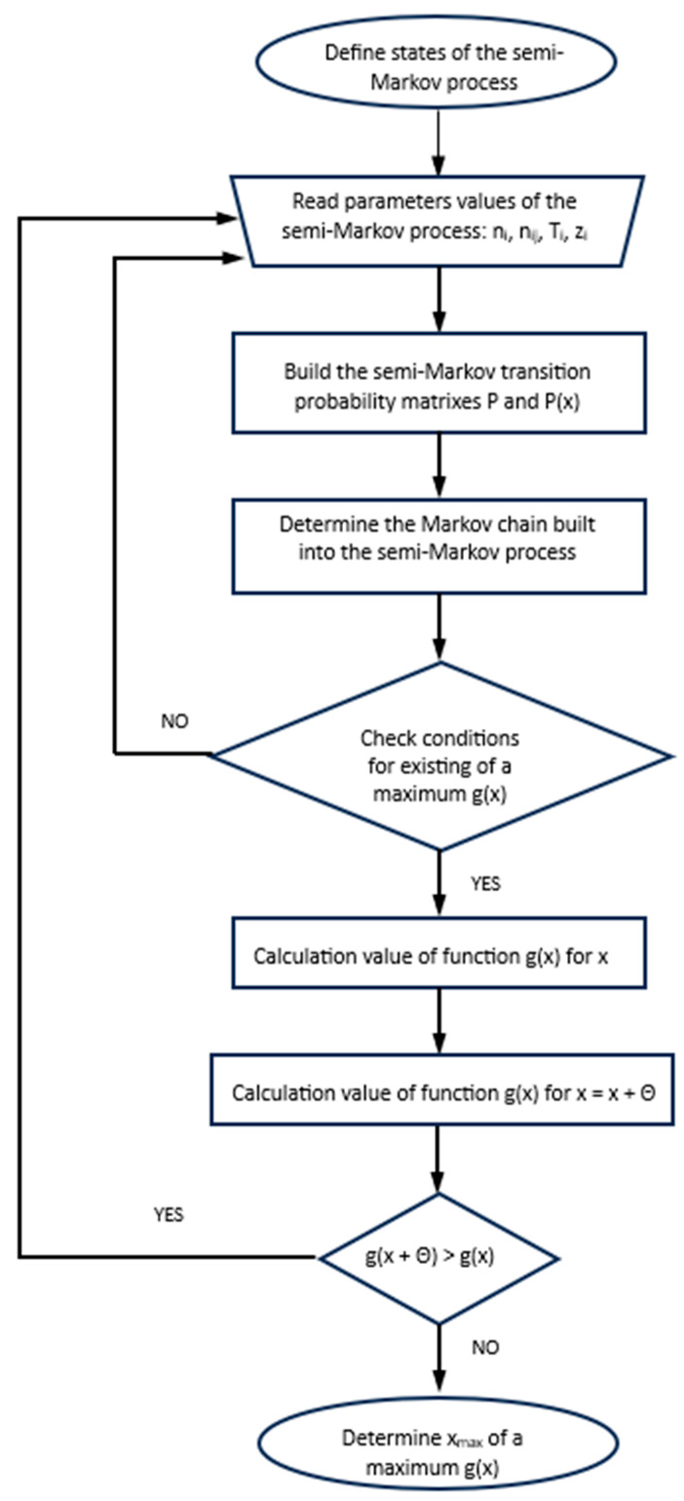
Figure 1. Block diagram of the modeling process.
Energies 17 00199 g001
Figure 2. Illustration depicting state transitions in the preventive maintenance system model based on the age of Enercon E82-2 wind turbines, with the state S = {1 to 6}.
Energies 17 00199 g002
Figure 3. Function g(x) graph: profit over time (1k PLN/day) within the preventive service x function (day), marked for the Weibull distribution: shape = 6.5, 8, 9.5, 11, and scale = 8 (lines a–d, respectively).
Energies 17 00199 g003
Figure 4. Function g(x) graph: wind turbine availability in the function of preventive service x (day) marked for the Weibull distribution: shape = 6.5, 8, 9.5, 11, and scale = 8 (lines a–d, respectively).
Energies 17 00199 g004
Figure 5. Function g(x) graph: profit over time (1k PLN/day) in the function of time preceding preventive service x (day), marked when the frequency of preventive service is the same as in example 1 (line a) and in the case of shortening the period of preventive maintenance by 15%, 25%, and 35%, respectively (lines b–d).
Energies 17 00199 g005
Figure 6. Function g(x) graph: availability of wind turbine in the function of time preceding preventive service x (day), marked when the frequency of preventive service is the same as in example 1 (line a) and in the case of shortening the period of preventive maintenance by 15%, 25%, and 35%, respectively, (lines b, c, and d).
Energies 17 00199 g006
Figure 7. Function g(x) graph: profit over time (1k PLN/day) in the function of time preceding preventive service x (day), marked for data from example 2 (scenario a) and scenarios b and c, for which the abilities of production and electric energy storing in state 2 of system modeling are estimated at 50% (line b) and 100% (line c).
Energies 17 00199 g007
Figure 8. Function g(x) graph: availability of wind turbine in the function of time preceding preventive service x (day), marked for data from example 2 (scenario a) and scenarios b and c, for which the abilities of production and electric energy storing in state 2 of system modeling are estimated at 50% (line b) and 100% (line c).
Energies 17 00199 g008
Disclaimer/Publisher’s Note: The statements, opinions and data contained in all publications are solely those of the individual author(s) and contributor(s) and not of MDPI and/or the editor(s). MDPI and/or the editor(s) disclaim responsibility for any injury to people or property resulting from any ideas, methods, instructions or products referred to in the content.