Non-Intrusive Reduced-Order Modeling Based on Parametrized Proper Orthogonal Decomposition

Abstract

A new non-intrusive reduced-order modeling method based on space-time parameter decoupling for parametrized time-dependent problems is proposed. This method requires the preparation of a database comprising high-fidelity solutions. The spatial bases are extracted from the database through first-level proper orthogonal decomposition (POD). The algebraic relationship between the time trajectory/parameter positions and the projection coefficient is described by the linear superposition of the second-level POD bases (temporal bases) and the second-level projection coefficients (parameter-dependent coefficients). This decomposition strategy decouples the space-time parameter effects, providing a stable foundation for fast predictions of parametrized time-dependent problems. The mappings between the parameter locations and the parameter-dependent coefficients are approximated as Gaussian process regression (GPR) models. The accuracy and efficiency of the PPOD-ROM are demonstrated through two numerical examples: flows past a cylinder and turbine flows with a clocking effect.

1. Introduction

In science and engineering, many time-dependent problems are governed by parametrized partial differential equations (PPDEs) [1,2], in which the parameters characterize the material properties, underlying geometry, source terms, boundary conditions, etc. [3]. It is often too expensive to run such high-fidelity, large-scale simulations with varying parameters. However, the intrinsic similarities among the parameter-dependent solutions can often be used to estimate the results for new parameters without repeated full-order solutions. Therefore, it is of great interest to derive parametrized reduced-order models (PROMs), which are more efficient but approximate the underlying high-resolution numerical simulations well [4,5].

PROMs aim to generate a low-rank approximation model that characterizes dynamical system responses with varying parameters [3]. Implemented in an offline–online paradigm [6], the reduced basis (RB) method has shown its ability to construct PROMs [2,7]. In the offline stage, a set of reduced bases is solved from a collection of full-order solutions (snapshots). Then, these RBs span a reduced subspace with a significantly smaller rank compared to high-fidelity dynamical systems. The greedy algorithm [8,9,10] and some modal decompositions, such as dynamic mode decomposition (DMD) [11,12,13] and proper orthogonal decomposition (POD) [14,15,16,17,18,19,20], are popular approaches for extracting the RBs. In the greedy algorithm, a set of snapshots is selected as the bases by utilizing an error estimator and an optimal criterion [21,22,23]. In the POD approach, the proper low-rank manifold is obtained by solving the eigenvectors from the database of full-order solutions. The DMD method attempts to find a low-dimensional approximation of the Koopman operator. Modal decomposition methods achieve a projection of complex systems onto a dynamical system with fewer degrees of freedom, although the principles for finding the low-dimensional space are different.

RB-based ROMs can generally be classified into two categories: intrusive and non-intrusive reduced-order models (NIROMs). For the intrusive models, the critical point is to fully decouple the online stage and the high-fidelity method, which is often tricky for non-linear problems with a non-affine dependence on parameters. Some methods, such as the empirical interpolation method [24,25], discrete empirical interpolation method [26], and function sampling method [27,28], have been proposed to address this issue. However, the application of intrusive ROMs is limited since modifications of the CFD source code are often required during the formation, which can be very complex for high-fidelity models. The modifications are only possible if the source code is available [29], especially for multi-parameter problems. The non-intrusive RB method is data-driven and enables flexibility for parametrized problems. Since evaluating a surrogate model involves only limited dimensions, the efficiency of the online stage can be ensured. The non-intrusive ROM approach has attracted significant attention recently, accompanied by the explosive development of machine learning. However, there are still some burning issues in NIROMs for parametrized time-dependent problems.

Yu et al. [30] pointed out that two critical issues must be addressed to model parametrized time-dependent problems. Firstly, the snapshot matrix becomes very large for problems with many time steps and parameter samples, leading to expensive singular-value decomposition (SVD). For this issue, methods such as the randomized SVD algorithm [31], fast adaptive cross-approximation [32], and local bases solutions method [33] have been used for large-scale problems. Beyond this, Wang et al. [34] applied POD twice to reduce the cost of global spatial bases for unsteady flow problems in the parameter domain. The second issue arises from the unsteadiness, which requires the regression models to predict the projection coefficients at an arbitrary time and with physical/geometrical parameters.

In recent years, there have been two strategies used to decouple space, time, and parameters in parametrized time-dependent problems. Most works try to extract spatial features based on POD offline and generate prediction models to map time/parameters with projection coefficients online. The parametric and temporal variables also need to be predicted online. Guo and Hesthaven [35] initially compressed snapshots with POD and separately decomposed the time and parameters with tensor decomposition based on SVD. The GPR models were used to map the parameters with time and parameter bases. Li et al. [36] extracted spatial bases with POD, and then the time trajectory was converted to a frequency-domain signal using a discrete Fourier transform (FFT). Artificial neural network (ANN) models in the frequency domain established the mappings between the parameters and projection coefficients. Xiao [37] applied POD along each trajectory, and then a two-level RBF interpolation method was employed. For new parameters, snapshots and POD bases were generated through first-level RBF interpolation. Then, a set of hypersurfaces corresponding to the POD bases along each trajectory was obtained through second-level RBF interpolation. In a recent work, the authors also demonstrated the ability of the DMD method to predict the temporal evolution of complex systems. Lukashevich et al. [38] predicted the evolution of the aggregation kinetics system using a small number of snapshots based on DMD. Duan [39] employed DMD technology to learn temporal features, enabling the prediction of full-order solutions at new time points.

Another approach is to extract spatial and temporal features from high-fidelity solutions with POD offline; regression models are only needed to map the relations between the projection coefficients and parameter input. Audouze et al. [33] proposed a two-level POD method to extract temporal and spatial bases from snapshots of dynamical systems offline. Then, the projection coefficients only depend on the flow parameters, leading to fewer requests for stability for regression models online. However, an auxiliary parabolic linear partial differential equation needs to be solved to enforce time-dependent boundary conditions, which are intrusive.

To further overcome these two issues, a parametrized, non-intrusive reduced-order model based on the parametric POD (PPOD) is proposed in this paper. The spatial bases are obtained from high-fidelity solutions using first-level POD, which is known as spatial decomposition. Then, the temporal bases are extracted from the first-level POD projection coefficients via second-level POD. This process is called temporal decomposition. The reduction is performed orderly through spatial and temporal decomposition, leading to high execution efficiency and a stable foundation for the predictions. The Gaussian process regression (GPR) [40,41] models are trained to map the second-level POD projection coefficients (parameter-dependent coefficients) to the flow parameters. In addition, the efficiency of the base extraction is further improved by using eigenvalue decomposition (EVD) instead of SVD in this work.

The remainder of this paper is organized as follows. Section 2 presents the parametrized reduction method for time-dependent problems, including the combination of the database, the EVD-based POD, and the PPOD theory. The GPR method and the framework of the PPOD-ROM are introduced in Section 3. Section 4 presents the numerical results and an efficiency analysis. Some conclusions are drawn in the Section 5.

2. Theory of Parametrized Reduction

The parametrized Navier–Stokes equations, governing unsteady flows, can be expressed in the conservative form:

$$\frac{\partial \mathit{u}(\mathit{x},t;\mathit{\alpha })}{\partial t}+\nabla \mathit{f}(\mathit{u}(\mathit{x},t;\mathit{\alpha });\mathit{\alpha })=\mathit{o}(\mathit{x},t,\mathit{u}(\mathit{x},t;\mathit{\alpha });\mathit{\alpha }),\forall (\mathit{x},t,\mathit{\alpha })\in \mathcal{S}\times \mathcal{T}\times \mathcal{P}$$

(1)

with some properly defined initial and boundary conditions. Here, $\mathit{u},\mathit{f},\mathit{o},\mathit{\alpha }$ are the vectors of the conserved variables, flux, source term, and parameters, respectively. $\mathcal{S}\subset {\mathbb{R}}^3,\mathcal{T}\subset {\mathbb{R}}^{+},\mathcal{P}\subset {\mathbb{R}}^c$ represent the physical space, time, and parameter domains, respectively. c is the dimension of the parameters. The scale of such a dynamical system for each given parameter set depends on the underlying mesh and the polynomial order of the discretization scheme. The full-order solutions for complex time-dependent problems often require immense numbers of cells, time steps, and iterations to guarantee the accuracy of the results, which limits the application in practical engineering. The intrinsic similarities among the parameter/time-dependent solutions can be used to estimate the solutions for new parameters without repeating high-fidelity evaluations.

The RB method is widely used for the reduction of complex parametrized problems. A reduced space is constructed by spanning a set of RB functions, and then an approximate solution to the parametrized problems can be sought efficiently in the reduced space. The greedy algorithm and POD are popular approaches for extracting RB functions from the database. However, the greedy procedure is unavailable for time-dependent problems with multi-parameters because there are no suitable error estimators or indicators for such problems [35]. Thus, this work uses the POD method to solve the RBs.

2.1. The Database of High-Fidelity Solutions

The solutions of Equation (1) with the variation of the parameters can be represented by a manifold $\mathcal{M}$, i.e., $\mathcal{M}=\left\{u\right(x,t;\mathit{\alpha }\left)\right\}$, and its discrete counterpart ${\mathcal{M}}_{N_s}=\left\{u_{N_s}(x,t;\mathit{\alpha })\right\}$, in which $N_s$ is the degrees of freedom of the physical space. Given a parameter set ${\mathcal{P}}_d=\left\{{\mathit{\alpha }}^{\left(1\right)},{\mathit{\alpha }}^{\left(2\right)},\cdots ,{\mathit{\alpha }}^{\left(N_p\right)}\right\}$, where $N_p$ is the number of parameter samples. The discrete high-fidelity solutions for the dynamical system in Equation (1) can be determined by running the solver with different parameters in ${\mathcal{P}}_d$. The full-order solutions with parameter ${\mathit{\alpha }}^{\left(k\right)}$ at time step $j\in [1,\cdots ,N_t]$ can be denoted as $u(x,t_j;{\mathit{\alpha }}^{\left(k\right)})\subset {\mathbb{R}}^{N_s}$, where $N_t$ is the number of time steps. Then, a matrix collecting snapshots with parameter ${\mathit{\alpha }}^{\left(k\right)}$ at all time steps is denoted as

$${\mathit{U}}^{\left(k\right)}=\left[u(x,t_1;{\mathit{\alpha }}^{\left(k\right)}),u(x,t_2;{\mathit{\alpha }}^{\left(k\right)}),\cdots ,u(x,t_{N_t};{\mathit{\alpha }}^{\left(k\right)})\right]\subset {\mathbb{R}}^{N_s\times N_t},$$

(2)

and the database of all $N_p$ parameter sets can be collected as

$$\mathit{U}=\left[{\mathit{U}}^{\left(1\right)},{\mathit{U}}^{\left(2\right)},\cdots ,{\mathit{U}}^{\left(N_p\right)}\right]\subset {\mathbb{R}}^{N_s\times N_{tp}},$$

(3)

where $N_{tp}=N_t\times N_p$.

2.2. The Improved Proper Orthogonal Decomposition

If the samples in ${\mathcal{P}}_d$ are proper, a subspace ${\mathcal{M}}_{{\mathcal{P}}_d}$ spanned by database $\mathit{U}$ contains sufficient information to characterize ${\mathcal{M}}_{N_s}$. The intrinsic similarities among the snapshots lead to the rank-deficient database $\mathit{U}$, which is the prerequisite for the RB method to work well. To construct a low-rank approximation for ${\mathcal{M}}_{{\mathcal{P}}_d}$ with rank $I\ll \min \left\{N_s,N_{tp}\right\}$, the POD is employed to extract a set of orthogonal bases $\mathbf{\Phi }=\left[{\mathit{\varphi }}_1,{\mathit{\varphi }}_2,\cdots ,{\mathit{\varphi }}_I\right]\in {\mathbb{R}}^{N_s\times I}$ from database $\mathit{U}$. There are two methods for solving POD bases: SVD and EVD. SVD, which can extract the POD bases conveniently, is widely used [33,35,41]. The SVD formula is denoted as

$$\mathit{U}=\mathit{W}\mathbf{\Lambda }{\mathit{Z}}^{\mathrm{T}}$$

(4)

with $\mathit{W}\in {\mathbb{R}}^{N_s\times N_s}$ and $\mathit{Z}\in {\mathbb{R}}^{N_{tp}\times N_{tp}}$ being orthogonal matrices, and the diagonal matrix $\mathbf{\Lambda }$ contains the singular values ${\lambda }_1\ge {\lambda }_2\ge \cdots \ge {\lambda }_{N_{tp}}$. Let $\mathit{V}\in {\mathbb{R}}^{N_s\times I}$ represent the set of all I orthogonal bases. POD bases minimize the projection error of $\mathit{U}$ onto the orthogonal bases $\mathit{V}$, and the projection error can be expressed as ${\sum }_{i=1}^{N_{tp}}{\parallel {\mathit{u}}_i-\mathit{V}{\mathit{V}}^{\mathrm{T}}{\mathit{u}}_i\parallel }^2$. The Schmidt–Eckart–Young theorem points out that the projection error can be evaluated using the $(I+1)$-th to the $N_{tp}$-th singular values as

$$\sum _{i=1}^{N_{tp}}\parallel {\mathit{u}}_i-\mathbf{\Phi }{\mathbf{\Phi }}^{\mathrm{T}}{\mathit{u}}_i{\parallel }^2=\sum _{i=1}^{N_{tp}}{\parallel {\mathit{u}}_i-\mathit{V}{\mathit{V}}^{\mathrm{T}}{\mathit{u}}_i\parallel }^2=\sum _{i=I+1}^{N_{tp}}{\lambda }_i^2.$$

(5)

Some studies define energy E as describing the reconstruction accuracy of the first I-th bases [37,42], and E can be expressed as:

$$E=\frac{{\sum }_{i=1}^I{\lambda }_i^2}{{\sum }_{i=1}^{N_{tp}}{\lambda }_i^2}.$$

(6)

The columns in $\mathit{W}$ corresponding to the top I singular values are the POD bases $\mathbf{\Phi }$.

In many engineering problems, the database is often very high-dimensional in one direction, i.e., $N_s\gg N_{tp}$, leading to profoundly inefficient SVD. EVD shows a better ability to deal with such issues. In fact, EVD and SVD are closely related. The left and right singular vectors in $\mathit{W}$ and $\mathit{Z}$ are also the orthonormal eigenvectors of $\mathit{U}{\mathit{U}}^{\mathrm{T}}$ and ${\mathit{U}}^{\mathrm{T}}\mathit{U}$, respectively [43]. The non-zero singular values of $\mathit{U}$ are the square roots of $\mathit{U}{\mathit{U}}^{\mathrm{T}}$ and ${\mathit{U}}^{\mathrm{T}}\mathit{U}$. Therefore, we can choose the smaller square matrices between $\mathit{U}{\mathit{U}}^{\mathrm{T}}$ and ${\mathit{U}}^{\mathrm{T}}\mathit{U}$ to efficiently perform EVD instead of SVD.

Considering that the dimension of ${\mathit{U}}^{\mathrm{T}}\mathit{U}\in {\mathbb{R}}^{N_{tp}\times N_{tp}}$ is far less than that of $\mathit{U}{\mathit{U}}^{\mathrm{T}}\in {\mathbb{R}}^{N_s\times N_s}$ in many actual engineering scenarios, the EVD is performed as

$${\mathit{U}}^{\mathrm{T}}\mathit{U}\mathbf{\Gamma }=\mathbf{\Sigma }\mathbf{\Gamma },$$

(7)

where $\mathbf{\Gamma }$ is equivalent to the right singular vectors $\mathit{Z}$ in Equation (4), and the diagonal matrix $\mathbf{\Sigma }$ contains the eigenvalues ${\sigma }_1\ge {\sigma }_2\ge \cdots \ge {\sigma }_{N_{tp}}$. Let $\mathit{S}=\mathrm{diag}\{\mathrm{sqrt}\left({\sigma }_1\right),$$\mathrm{sqrt}\left({\sigma }_2\right),$$\cdots ,$$\mathrm{sqrt}\left({\sigma }_{N_{tp}}\right)\}$, so $\mathit{S}$ is equal to the singular-value matrix $\mathbf{\Lambda }$. The approximate left singular vector matrix $\widehat{\mathit{W}}$ can be solved using the inverse operations of Equation (4) as

$$\widehat{\mathit{W}}=\mathit{U}{\left({\mathbf{\Gamma }}^{\mathrm{T}}\right)}^{-1}{\mathit{S}}^{-1}=\mathit{U}\mathbf{\Gamma }{\mathit{S}}^{-1},$$

(8)

where $\mathbf{\Gamma }$ is an orthogonal matrix and $\mathit{S}$ is a diagonal matrix, so the inverse operation in Equation (8) is easy to run. The POD bases $\mathbf{\Phi }\in {\mathbb{R}}^{N_s\times I}$ are taken from the first I columns of $\widehat{\mathit{W}}$, and the projection coefficients are defined as $\mathit{A}={\mathbf{\Phi }}^{\mathrm{T}}\mathit{U}$. Due to its high efficiency, EVD is used to extract the POD bases in this work.

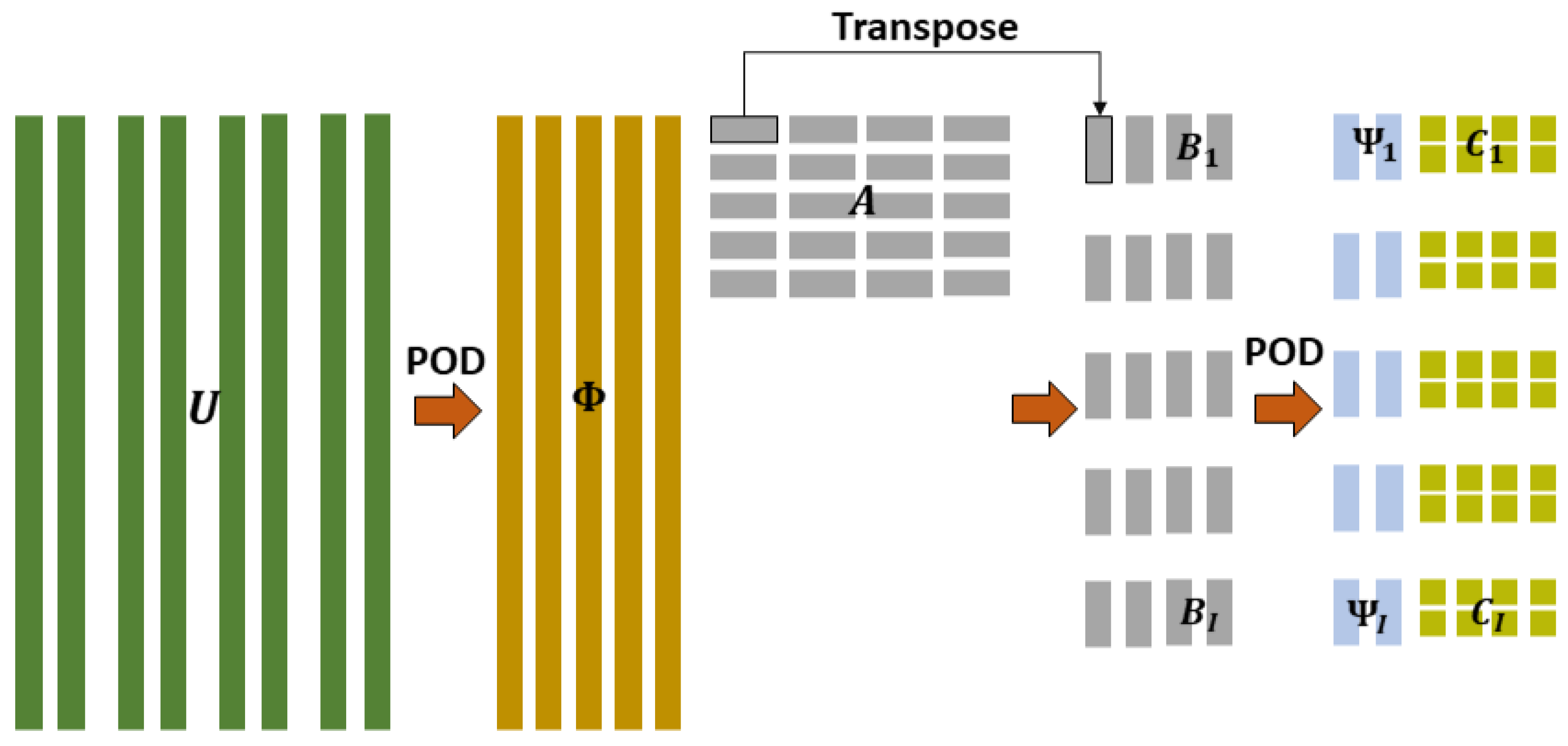
2.3. Reduction Based on Parametric POD

For parametrized time-dependent problems, the projection coefficients of the classical POD method evolve substantially over time, often leading to difficulties in regressions [30,41]. In this work, a new reduction approach for parametrized time-dependent problems, namely parametric POD (PPOD), is proposed to ensure reliable and efficient prediction results in regression.

The approximation for parametrized time-dependent problems is denoted as

$$\begin{array}{cc}\hfill u(x,t,{\mathit{\alpha }}^{\left(k\right)})=& \sum _{i=1}^I{a}_i(t,{\mathit{\alpha }}^{\left(k\right)}){\varphi }_i\left(x\right)\hfill \\ \hfill =& \sum _{i=1}^I\sum _{j=1}^J{c}_{ij}\left({\mathit{\alpha }}^{\left(k\right)}\right){\psi }_{ij}\left(t\right){\varphi }_i\left(x\right),\hfill \end{array}$$

(9)

where I is the truncation rank, ${\varphi }_i\left(x\right)$ is the i-th spatial basis, and $a_i(t,{\mathit{\alpha }}^{\left(k\right)})$ is the first-level projection coefficient. ${\sigma }_i$ is the i-th eigenvalue corresponding to the i-th basis, which is used to represent the reduction accuracy below. Since the high-fidelity data are decomposed into a linear superposition of spatial bases and first-level projection coefficients, this reduction is named spatial decomposition. In the next process, POD can be performed again to decouple the algebraic correlation of the parameter locations and time trajectory in $a_i(t,{\mathit{\alpha }}^{\left(k\right)})$. $a_i(t,{\mathit{\alpha }}^{\left(k\right)})$ can be decomposed using the temporal bases and the second-level projection coefficients (parameter-dependent coefficients). J is the second truncation rank, ${\psi }_{ij}\left(t\right)$ is the j-th temporal basis, and $c_{ij}\left({\mathit{\alpha }}^{\left(k\right)}\right)$ is the j-th parameter-dependent coefficients corresponding to the i-th spatial basis. ${ϵ}_{ij}$ is the eigenvalue corresponding to the i-th spatial basis and the j-th temporal basis, which is used in the assessment of the second-level truncation error.

By transforming the high-fidelity solutions into parameter-dependent coefficients, the complexity of establishing regression models between flow parameters and coefficients has been significantly reduced. A discussion on implementing the decompositions of Equation (9) in a matrix operation can be found below. The matrix of first-level projection coefficients $\mathit{A}$, obtained by projecting $\mathit{U}$ onto the space spanned by spatial bases $\mathbf{\Phi }$, is denoted as

$$\mathit{A}={\mathbf{\Phi }}^{\mathrm{T}}\mathit{U}\subset {\mathbb{R}}^{I\times N_{tp}}.$$

(10)

The i-th coefficients of the spatial decomposition, i.e., the i-th row vector in $\mathit{A}$, is denoted as

$$\mathit{A}(i,:)=\left[\begin{array}{cccc}{\mathit{a}}_i(t_1:t_{N_t};{\mathit{\alpha }}^{\left(1\right)})|& {\mathit{a}}_i(t_1:t_{N_t};{\mathit{\alpha }}^{\left(2\right)})|& \cdots |& {\mathit{a}}_i(t_1:t_{N_t};{\mathit{\alpha }}^{\left(N_p\right)})\end{array}\right].$$

(11)

$\mathit{A}$ characterizes the time trajectory of dynamic system responses with varying parameters. The intrinsic similarity between the row vectors in $\mathit{A}$ can be used to estimate the time trajectory corresponding to the parameters. A database of the i-th first-level projection coefficients can be combined as

$${\mathit{B}}_i=\left[\begin{array}{cccc}{\mathit{a}}_i{(t_1:t_{N_t};{\mathit{\alpha }}^{\left(1\right)})}^{\mathrm{T}}|& {\mathit{a}}_i{(t_1:t_{N_t};{\mathit{\alpha }}^{\left(2\right)})}^{\mathrm{T}}|& \cdots |& {\mathit{a}}_i{(t_1:t_{N_t};{\mathit{\alpha }}^{\left(N_p\right)})}^{\mathrm{T}}\end{array}\right]\subset {\mathbb{R}}^{N_t\times N_p}.$$

(12)

The algebraic effects of parameters on the time trajectory in ${\mathit{B}}_i$ can be reduced by seeking a more appropriate subspace using POD. The reduction can be described as ${\mathit{B}}_i={\mathbf{\Psi }}_i{\mathit{C}}_i$, where the j-th column in ${\mathbf{\Psi }}_i\subset {\mathbb{R}}^{N_t\times J}$ is ${\mathit{\psi }}_{ij}\left(t\right)$ and the j-th row in ${\mathit{C}}_i\subset {\mathbb{R}}^{J\times N_p}$ is $c_{ij}\left({\mathit{\alpha }}^{\left(k\right)}\right)$, corresponding to the characters in Equation (9). The temporal decomposition is achieved by performing the above procedure for all ${\mathit{B}}_i,i\in [1,I]$. Figure 1 gives a visual description of the PPOD process.

The relative error of spatial and temporal decompositions in PPOD is estimated using error estimation based on eigenvalues. Following the two truncations in the PPOD, the relative error for the recovery of spatial decomposition for database $\mathit{U}$ is expressed as

$$\begin{array}{cc}\hfill e_{1st}^2=& \frac{{\sum }_{m=1}^{N_t}{\sum }_{k=1}^{N_p}{\parallel \mathit{u}(t_m,{\mathit{\alpha }}^{\left(k\right)})-{\sum }_{i=1}^I{a}_i(t_m,{\mathit{\alpha }}^{\left(k\right)}){\mathit{\varphi }}_i\parallel }^2}{{\displaystyle \sum _{\mathit{u}\in \mathit{U}}}{\parallel \mathit{u}\parallel }^2}\hfill \\ \hfill =& \frac{{\displaystyle \sum _{\mathit{u}\in \mathit{U}}}{\parallel \mathit{u}-\mathbf{\Phi }{\mathbf{\Phi }}^{\mathrm{T}}\mathit{u}\parallel }^2}{{\displaystyle \sum _{\mathit{u}\in \mathit{U}}}{\parallel \mathit{u}\parallel }^2}=\frac{{\sum }_{i=I+1}^{N_{tp}}{\sigma }_i}{{\sum }_{i=1}^{N_{tp}}{\sigma }_i}.\hfill \end{array}$$

(13)

For temporal decomposition of ${\mathit{B}}_i,i\in [1,I]$, the truncation error can be defined as

$$\begin{array}{cc}\hfill e_{2nd,i}^2=& \frac{{\sum }_{k=1}^{N_p}{\parallel \mathit{b}\left({\mathit{\alpha }}^{\left(k\right)}\right)-{\sum }_{j=1}^J{c}_j\left({\mathit{\alpha }}^{\left(k\right)}\right){\mathbf{\psi }}_{ij}\parallel }^2}{{\displaystyle \sum _{\mathit{b}\in {\mathit{B}}_i}}{\parallel \mathit{b}\parallel }^2}\hfill \\ \hfill =& \frac{{\displaystyle \sum _{\mathit{b}\in {\mathit{B}}_i}}{\parallel \mathit{b}-{\mathbf{\Psi }}_i{\mathbf{\Psi }}_i^{\mathrm{T}}\mathit{b}\parallel }^2}{{\displaystyle \sum _{\mathit{b}\in {\mathit{B}}_i}}{\parallel \mathit{b}\parallel }^2}=\frac{{\sum }_{j=J+1}^{N_p}{ϵ}_{ij}}{{\sum }_{j=1}^{N_p}{ϵ}_{ij}},\hfill \end{array}$$

(14)

thus, the total truncation relative error e of PPOD for the recovery can be denoted as

$$e=1-\sum _{i=1}^I\left(\frac{{\sigma }_i}{{\sum }_{k=1}^{N_{tp}}{\sigma }_k}\times \frac{{\sum }_{j=1}^J{ϵ}_{ij}}{{\sum }_{j=1}^{N_p}{ϵ}_{ij}}\right).$$

(15)

3. Parametrized ROMs Based on PPOD

This paper aims to efficiently and thoroughly reduce system dimensions (compressing both space and time) by predicting a minimal set of decoupled variables (parameter-dependent) to enhance the framework’s operational efficiency and accuracy. PPOD meets these requirements, eliminating the need for overly complex prediction models. This extreme dimensionality reduction-prediction framework makes it convenient for engineers to replace different prediction models according to practical needs. In this work, a simple GPR model was chosen to validate the accuracy and application potential of the proposed framework. This section focuses on the framework based on the PPOD-GPR models and briefly introduces GPR.

3.1. Gaussian Process Regression Models

Regression is concerned with the prediction of a continuous variable of interest through the construction of a model from a set of observational data [40,44]. Define ${\mathcal{P}}_{tr}$ = $\{({\mathit{x}}_i,y_i)$: $i=1,2,\dots ,N\}$ as the training set of N observations, where input ${\mathit{x}}_i\in {\mathcal{P}}_{tr}\subset {\mathbb{R}}^c$ consists of c entries, and $y_i\in \mathbb{R}$ is the output corresponding to ${\mathit{x}}_i$. In GPR models, we assume that the observed input-output pairs follow some regression function $f:\mathcal{P}\to \mathbb{R}$, which is defined as a Gaussian process (GP). When given a new input, the corresponding output can be predicted by this GPR model.

GPR models are non-parametrized kernel-based probabilistic models, and the linear regression model is of the form

$$y=x^T\beta +ϵ$$

(16)

where $ϵ\sim \mathcal{N}(0,{\sigma }^2)$. GPR models can describe a response by introducing latent functions $f\left(x\right)$ from a Gaussian process and basis function h. A GP is a set of random variables, and any finite number of them obeys a joint Gaussian distribution. It can be defined by its mean function $m\left(x\right)$ and covariance function, $k(x,x^{{}^{\prime }})$, where $m\left(x\right)=E\left(f\right(x\left)\right)$ and $k(x,x^{{}^{\prime }})=\mathrm{Cov}(f\left(x\right),f{\left(x\right)}^{{}^{\prime }})$. Then, the regression model is of the form

$$y=h{\left(x\right)}^T\beta +f\left(x\right)$$

(17)

where $f\left(x\right)\sim \mathrm{GP}(0,k(x,x^{{}^{\prime }}))$ and $h\left(x\right)$ are a collection of basis functions defined in $\mathcal{P}$, and $\beta$ represents the corresponding combination coefficients. Generally, there are many options for $k(x,x^{{}^{\prime }})$. In this work, an automatic relevance determination (ARD) squared exponential (SE) kernel is used for the solution of the covariance function:

$$k(\mathit{x},{\mathit{x}}^{{}^{\prime }})=s_f^{2}exp\left(-\frac{1}{2}\sum _{n=1}^d\frac{{(x_m-x_m^{{}^{\prime }})}^2}{l_m^2}\right)$$

(18)

where $s_f^2$ represents the width coefficients, and $l_m$ is the individual correlated length scale for each input. For a number of points of input, the joint Gaussian can be defined as follows,

$$\mathit{y}|\mathit{X}\sim \mathcal{N}\left(m\left(\mathit{X}\right),\mathit{K}\right)$$

(19)

where $\mathit{K}=\mathrm{cov}\left(\mathit{y}\right|\mathit{X})=k(\mathit{X},\mathit{X})+{\sigma }^2{\mathit{I}}_N$, $\mathit{y}={\left[y_1,y_2,\dots ,y_n\right]}^T$, and $\mathit{X}=\left[{\mathit{x}}_1,{\mathit{x}}_2,\dots ,{\mathit{x}}_n\right]$. ${\mathit{I}}_N$ is the N-dimensional unit matrix.

To predict the noise-free output $\widehat{f\left(\mathit{\alpha }\right)}$ for a new input $\mathit{\alpha }$ using this regression model, we combine the information of the training set with the predictions of test samples to form the joint density of observations $\mathit{y}$ and noiseless test output $\widehat{f\left(\mathit{\alpha }\right)}$. Then, the posterior predictive distribution, in the form of a new GP, can be obtained through the standard rules for conditioning Gaussians:

$$\widehat{f\left(\mathit{\alpha }\right)}|\mathit{\alpha },\mathit{X},\mathit{y}\sim \mathrm{GP}\left(\hat{m}\left(\mathit{\alpha }\right),\hat{z}(\mathit{\alpha },{\mathit{\alpha }}^{{}^{\prime }})\right)$$

(20)

where

$$\hat{m}\left(\mathit{\alpha }\right)=m\left(\mathit{\alpha }\right)+k(\mathit{\alpha },\mathit{X}){\mathit{K}}^{-1}(\mathit{y}-m\left(\mathit{X}\right))$$

(21)

and

$$\hat{z}(\mathit{\alpha },{\mathit{\alpha }}^{{}^{\prime }})=k(\mathit{\alpha },{\mathit{\alpha }}^{{}^{\prime }})-k(\mathit{\alpha },\mathit{X}){\mathit{K}}^{-1}k(\mathit{X},{\mathit{\alpha }}^{{}^{\prime }})$$

(22)

The required parameters can be solved using an empirical Bayesian approach that maximizes the likelihood. By setting the hyperparameters $\mathit{\theta }=[{\beta }_1,{\beta }_2,\dots ,{\beta }_m,l_1,l_2,\dots ,l_d,s_f,{\sigma }_s]$, the optimal $\mathit{\theta }$ can be determined by solving this maximization problem using a standard gradient-based optimizer:

$$\begin{array}{cc}\hfill \mathit{\theta }& =\underset{\theta }{argmax}logp\left(\mathit{y}\right|\mathit{X},\mathit{\theta })\hfill \\ \hfill & =argmax\left\{-\frac{1}{2}{(\mathit{y}-{\mathit{\beta }}^T\mathit{H}\left(\mathit{X}\right))}^T{\mathit{K}}^{-1}\left(\mathit{\theta }\right)(\mathit{y}-{\mathit{\beta }}^T\mathit{H}\left(\mathit{X}\right))-\frac{1}{2}log\left|\mathit{K}\left(\mathit{\theta }\right)\right|-\frac{N}{2}log\left(2\pi \right)\right\}\hfill \end{array}$$

(23)

where $p\left(\mathit{y}\right|\mathit{X},\mathit{\theta })$ is the conditional density function of $\mathit{y}$ given $\mathit{X}$ with $\mathit{\theta }$, which can be obtained through the marginal likelihood,

$$p(\mathit{y}|\mathit{X},\mathit{\theta })=\int p(\mathit{y}|\mathit{f},\mathit{X},\mathit{\theta })p(\mathit{f}|\mathit{X},\mathit{\theta })d\mathit{f}$$

(24)

In this work, the GPR model simply uses $\mathit{H}\left(\mathit{x}\right)=1$ as the basis function.

3.2. Framework of PPOD-ROMs

In non-intrusive ROMs, the approximate solutions of a new parameter value ${\mathit{\alpha }}^{*}$ are determined by evaluating a regression model online. For parameter time-dependent problems, the input of the regression model is the parameter ${\mathit{\alpha }}^{*}$, and the outputs are the projection coefficients online. We assume that an ideal regression $\mathit{\pi }$ maps the input $\mathit{\alpha }$ to the projections coefficients ${\mathit{C}}_i,i\in [1,I]$, described as $\mathit{\alpha }\to {\mathit{C}}_i$. A GPR model is generated to act as an approximation ${\hat{\mathit{\pi }}}_{\mathrm{PPOD}}$ of the map $\mathit{\pi }$ for ${\mathit{C}}_i$. Given a new parameter ${\mathit{\alpha }}^{*}$, the projection coefficients are obtained by evaluating ${\hat{\mathit{\pi }}}_{\mathrm{PPOD}}$, i.e., ${\mathit{C}}_i^{*}={\hat{\mathit{\pi }}}_{\mathrm{PPOD}}{\mathit{\alpha }}^{*}$, and the coefficients ${\mathit{B}}_i^{*}$ can be obtained by ${\mathit{B}}_i^{*}={\mathbf{\Psi }}_i{\mathit{C}}_i^{*}$. By combining the matrix ${\mathit{B}}_i^{*},i\in [1,I]$ to ${\mathit{A}}^{*}$, the approximated solution can be determined by ${\mathit{U}}^{*}=\mathbf{\Phi }{\mathit{A}}^{*}$. The PPOD-ROM algorithms are described in Algorithm 1.

Algorithm 1 ROM based on PPOD and GPR for parametrized time-dependent problems

1: procedure $\text{PPOD-OFFLINE}$($\mathit{U},\mathit{\alpha },e_{1st}^2,e_{2nd}^2$) 2:     Solving the spatial bases $\left[\mathbf{\Phi },I\right]=\mathrm{POD}(\mathit{U},e_{1st}^2)$ 3:     Determining the first-level projection coefficients by $\mathit{A}={\Phi }^{\mathrm{T}}\mathit{U}$ 4:     Assembling ${\mathit{B}}_i=\left[{\mathit{a}}_i{(t_1:t_{N_t};{\mathit{\alpha }}^{\left(1\right)})}^{\mathrm{T}}|{\mathit{a}}_i{(t_1:t_{N_t};{\mathit{\alpha }}^{\left(2\right)})}^{\mathrm{T}}|\cdots |{\mathit{a}}_i{(t_1:t_{N_t};{\mathit{\alpha }}^{\left(N_p\right)})}^{\mathrm{T}}\right],i\in [1,I]$, where ${\mathit{a}}_i$ is the i-th-order projection coefficient of $\mathit{A}$ 5:     Solving the temporal bases $[{\mathbf{\Psi }}_i,J]=\mathrm{POD}({\mathit{B}}_i,e_{2nd}^2)$ 6:     Determining the parameter-dependent coefficients by ${\mathit{C}}_i={\mathbf{\Psi }}_i^{\mathrm{T}}{\mathit{B}}_i$ 7:     Training the mapping relationship $\hat{\mathit{\pi }}$ between $\mathit{\alpha }$ and ${\mathit{C}}_i$ using a GPR model 8:     return $\left[\mathbf{\Phi },{\mathbf{\Psi }}_i,{\mathit{C}}_i,\hat{\mathit{\pi }}\right]$ 9: end procedure 1: procedure ROM-ONLINE($\mathbf{\Phi },{\mathbf{\Psi }}_i,{\mathit{C}}_i,{\mathit{\alpha }}^{*},i\in [1,I]$) 2:     Evaluating outputs ${\mathit{C}}_i^{*}=\hat{\mathit{\pi }}{\mathit{\alpha }}^{*}$ of the GPR for new inputs ${\mathit{\alpha }}^{*}$ 3:     Computing approximate coefficients ${\mathit{B}}_i^{*}=\mathbf{\Psi }{\mathit{C}}_i^{*}$ 4:     Assembling ${\mathit{A}}^{*}$ from ${\mathit{B}}_i^{*}$ 5:     Solving the approximate solution ${\mathit{U}}^{*}=\mathbf{\Phi }{\mathit{A}}^{*}$ 6:     return ${\mathit{U}}^{*}$ 7: end procedure

4. Numerical Examples

In this section, two numerical results are presented to validate the effectiveness of the proposed parametrized ROM. In the first numerical case, incompressible flows past a cylinder are solved. The predictive power of transient static pressure is demonstrated as the boundary condition (inlet velocity), and model parameter (density) vary. The second case involves two stages of compressible turbine flows with varying geometric boundaries (clocking positions). The unsteady static pressure and Mach number are considered in this case.

4.1. Flows Past a Cylinder

Flows past a cylinder are numerically simulated in the first example. The left boundary of the domain is the inlet, and an inlet velocity drives the fluid dynamics of the flow. The flow is allowed to pass through the right boundary of the domain with zero gradient for variables in the outflow. The periodic boundary conditions are applied to the lower and upper edges, and the no-slip boundary conditions are applied to the wall of the cylinder. The k-$\omega$ SST turbulence model is chosen to close the time-averaged Navier–Stokes equations. The COUPLED algorithm is utilized for the coupling of pressure and velocity during the solution of the momentum and pressure-based continuity equations. The QUICK scheme for discretizing convective terms is utilized to enhance solution accuracy. The second-order implicit method is chosen for transient formulation. The time step is determined based on the estimated periodic of the Karman vortex, as outlined in Equation (26).

The Reynolds number is an important parameter used to characterize turbulence. For credible 2D simulations, the Reynolds number is varied from 100 to 1500 in this example. The Reynolds number is defined as

$$Re=\frac{U_{vel}D\rho }{\mu }.$$

(25)

The diameter of the cylinder is set as $D=1$, the viscosity of the fluid is set as $\mu =1$, and the inlet velocity and density are set in the following range,

$$U_{\mathrm{vel}}\in \left[1,5\right],\rho \in \left[100,300\right].$$

In this case, Latin hypercube sampling (LHS) is used to design the experiment for the inlet velocity and density. The total number of samples is split into training and testing sets to meet the requirements of randomness and mutual exclusivity. There are 51 samples selected by LHS, of which 45 are treated as training samples, and the others are testing samples. The training and testing samples are shown in Figure 2. The solution snapshots at the training and testing parameter instances were obtained by running the CFD model.

For classic flows past a cylinder, the temporal period can be determined approximately by the Stourhal number $S_r$. The vortex-shedding period T or frequency f can be approximated by $S_r$ and inlet velocity $U_{\mathrm{vel}}$ as follows:

$$T=\frac{1}{f}=\frac{D}{S_r{U}_{\mathrm{vel}}},$$

(26)

where $S_r$ is usually 0.21 at a low $Re$ for the flows past a cylinder example. The a priori vortex-shedding period helps to determine the correct time-sampling steps with varying inlet velocities. In these CFD simulations, the vortex-shedding periods are divided into 42 steps to extract the flow structures.

The spatial and temporal POD energy, defined in Equation (6), is presented in Figure 3. Sharp drops in the first few eigenvalues, which reflect the bases associated with larger eigenvalues, can capture more information in the space spanned by $\mathit{U}$ and $\mathit{B}=[{\mathit{B}}_1,{\mathit{B}}_2,\cdots ,{\mathit{B}}_I]$. The results reflect that the linear superposition by a few bases can approximate the features included in $\mathit{U}$ and ${\mathit{B}}_i,i\in [1,I]$. The above findings show that the flow characteristic is not converted dramatically with variations in the inlet velocity and density of flows past a cylinder. Some spatial bases are shown in Figure 4. To demonstrate reduction effectiveness, the relative truncation error, defined in Equation (15), with varying truncation orders, is shown in

Table 1. The relative truncation error by the PPOD-ROM for flows past a cylinder.

Truncation Orders	${\mathit{e}}_{1\mathit{st}}^2$	${\mathit{e}}_{2\mathit{nd}}^2$	e
$I=1,J=1$	0.101	0.003	0.103
$I=3,J=3$	0.003	0.001	0.004
$I=10,J=10$	0.001	0.000	0.001
$I=30,J=30$	0.000	0.000	0.000

. It indicates that the relative truncation error could decrease to critically low levels with only a limited increase in the bases. The first four temporal bases, corresponding to the first four spatial bases, are shown in Figure 5. It can be seen that most temporal bases corresponding to all four spatial bases are periodic, which reflects the time history of the vortex-shedding period.

In this example, the PPOD-ROMs with $3\times 3$ (3 spatial bases and 3 temporal bases), $10\times 10$, and $30\times 30$ bases are constructed to predict the static pressure in the domain. The unsteady flow fields with testing parameters ($U_{\mathrm{vel}}=2.5,\rho =240$) at time $t=0.25$ T and $t=$ T are presented in Figure 6. It can be seen that the $3\times 3$ PPOD-ROM can still capture the dominant flow structure, while there are some visual differences between the results of the CFD and the PPOD-ROM. With the increasing number of spatial and temporal bases, more details of the flow structures can be captured. This can be confirmed by observing the absolute pressure errors shown in Figure 7. For predicting transient field problems, the relative error might be amplified due to the true values approaching zero being in the denominator. Therefore, the use of absolute error and assessing predictive performance based on the maximum error in comparison with the location of maximum oscillations in the high-fidelity numerical field is reasonable.

To evaluate the maximum error of the PPOD-ROM throughout the whole vortex-shedding cycle, monitors A and B are arranged at positions with poor prediction in the field. The monitor locations are shown in Figure 7f. Figure 8 reveals that the results of the PPOD-ROM agree with those of CFD for peak and variation trends in the domain where the maximum error occurs, and only slight differences are observed in phase. The subtle differences in phase are the primary reason for the transient field errors observed in Figure 7.

A global error factor encompassing all testing samples in the full-time cycle is proposed to validate the generalization ability of the PPOD-ROM, which is defined as

$$r_p=\frac{1}{N_t}\sum _{t=1}^{N_t}\frac{\sqrt{\frac{1}{N_s}{\sum }_{n=1}^{N_s}{(u_{n,t,p}^{{}^{\prime }}-u_{n,t,p})}^2}}{\sqrt{\frac{1}{N_s}{\sum }_{n=1}^{N_s}{(u_{n,t,p}-{\overline{u}}_n)}^2}},$$

(27)

where $u_{n,t,p}$ and $u_{n,t,p}^{{}^{\prime }}$ are the solutions at the n-th cell, t time, and p parameter location solved by the PPOD-ROMs and CFD model, respectively. $\overline{\mathit{u}}=\frac{1}{N_t{N}_p}{\sum }_{p=1}^{N_p}{\sum }_{t=1}^{N_t}{\mathit{u}}_{t,p}$ denotes the average snapshot of the database, and ${\overline{u}}_n$ is the value on the n-th cell of $\overline{\mathit{u}}$. This is also a critical metric for assessing the temporal integration prediction accuracy of the model at different parameter locations. As shown in Figure 9, $r_p$ for all test samples is less than 0.03. The relatively small differences in $r_p$ among the prediction points suggest that the model can achieve accuracy similar to what is shown in Figure 6 and Figure 8 at other parameter points as well. Additionally, the scattering of test points in space indicates the stability of the model across the entire parameter domain.

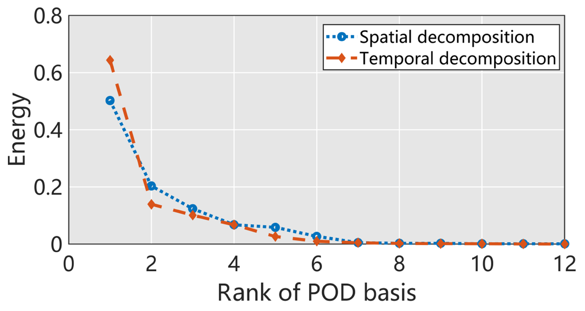
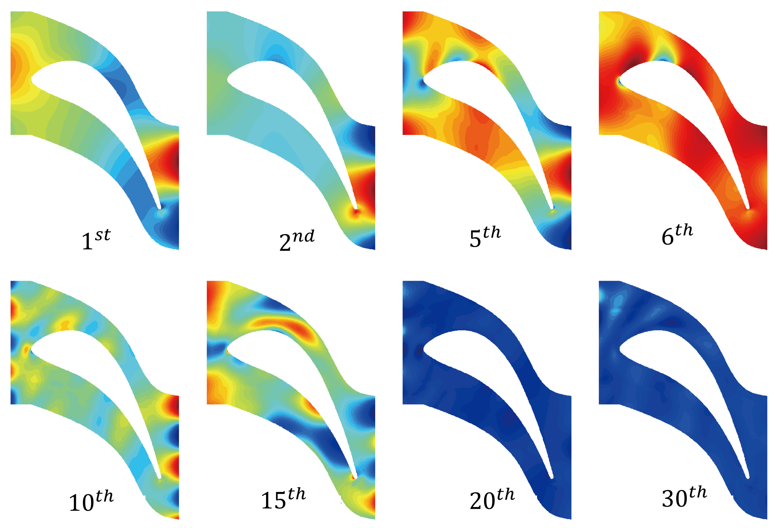
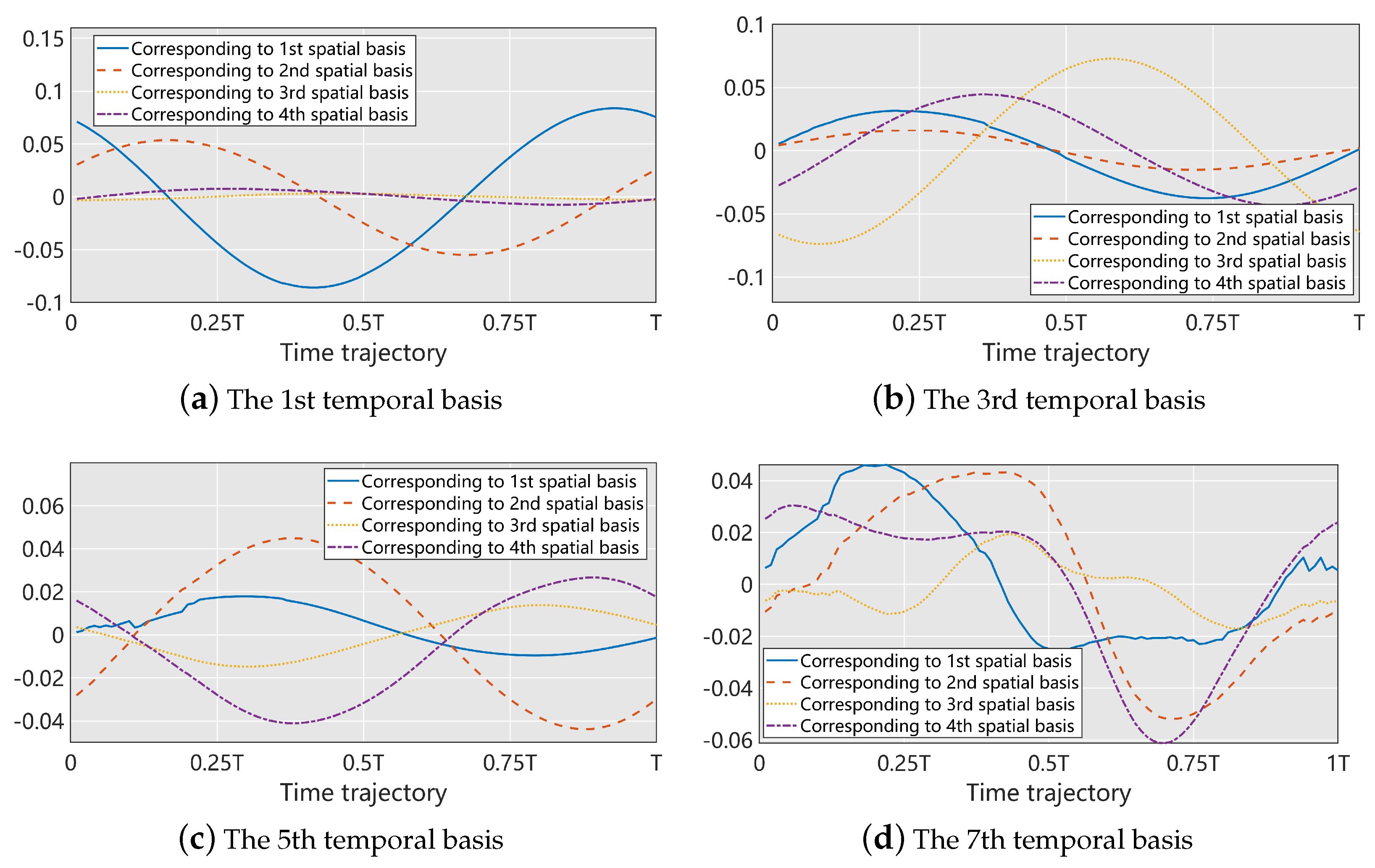
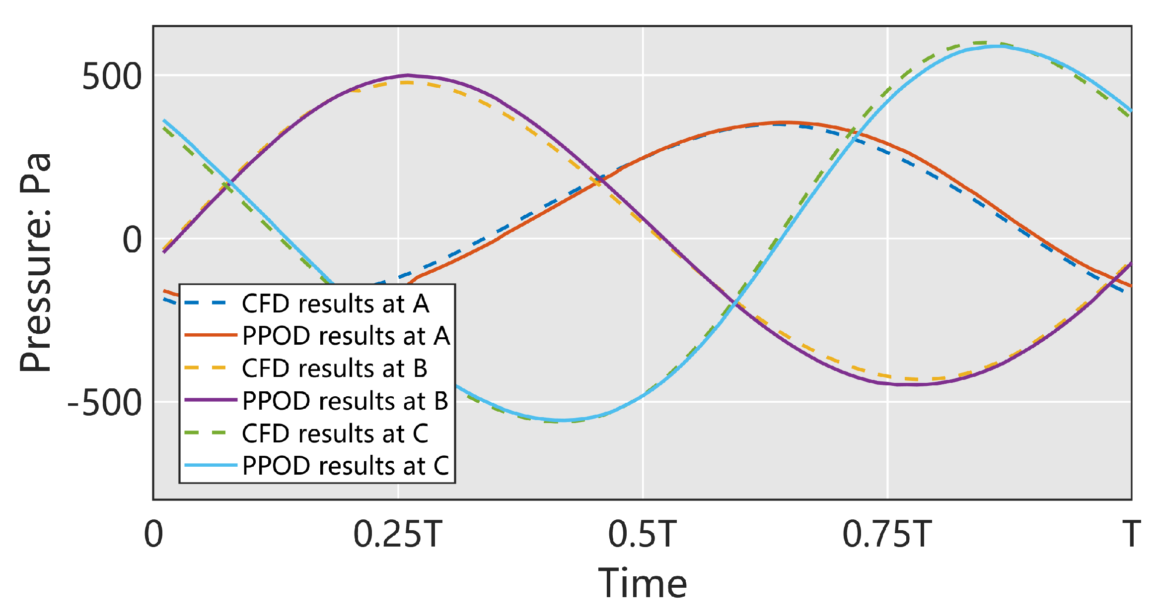
4.2. Turbine Flows with Clocking Effect

The interaction between rotors and stators causes an inherently unsteady flow in multistage turbo-machines, which is the primary source of unsteady excitation on the blades. The circumferential phase difference between adjacent stators or rotors in turbo-machines causes the mixing loss and energy change variation, intensifying the unsteady characteristics of the flow field. This phenomenon was named the clocking effect in previous studies [45,46,47,48].

A two-stage turbine considering the clocking effect is shown in Figure 10. The clocking position of stators and rotors (the relative clocking position between the first-stage stator and second-stage stator, as well as the first-stage rotor and second-stage rotor), i.e., CS0–CS3 (relative position of stators) and CR0–CR3 (relative position of rotors), will cause variations in unsteady flow structure. In this example, a PPOD-ROM is constructed to describe the non-linear relation between the clocking positions and unsteady fields.

The turbulence model and the spatial-temporal discretization method utilized in this simulation case are consistent with case 1. The difference lies in enabling the energy equation for compressible flow calculations, with the working fluid assumed to be an ideal gas. The time step is set to one percent of the rotor passing through one stator channel period, which is 4.18 × 10${}^{-6}$. The necessary flow parameters and boundary conditions are listed in

Table 2. Boundary conditions of the two-stage turbine.

CFD Settings	Value
The pitch of blade (m)	0.0418
Speed of rotors (m/s)	100
The total pressure of inlet (Pa)	166,600
The temperature of inlet (K)	309
The pressure of outlet (Pa)	101,325
The temperature of outlet (K)	309

. ${\alpha }_1$ and ${\alpha }_2$ denote the clocking positions of the stators and rotors, respectively. Since the pitch between adjacent blades is 0.0418 m, the clocking positions of the stator blades as variable ${\alpha }_1$ and the rotor blades as variable ${\alpha }_2$ are within the range $\left[0,0.0418\right]$. Unlike case 1, a total of 30 parameter sets are used to train and test the PPOD-ROM for turbine flows, which are generated using the Sobol sampling technique [49]. The distribution of samples is shown in Figure 11. The Sobol method ensures that the sampled points are uniform across the parameter space. The use of different sampling methods here aims to observe the applicability of the present prediction framework to sampling variations.

Generally, the source of unsteady excitations on turbine blades is the wakes from upstream and potential flows from downstream. The variations in pressure in the R1 or S2 region would be more violent compared to other regions by adjusting the circumferential positions of the rotor and stator blades. Thus, the unsteady static pressure field in the S2 region is used to evaluate the prediction accuracy of the PPOD-ROMs. For the flow in a compressor, the static pressure of the flow remains relatively stable, i.e., the unsteady pressure caused by wake flows and potential flows is often several orders less than the time-averaged flow. However, the time-varying pressure oscillation is the primary unsteady excitation of blade dynamics, which can cause blade fracture. Thus, it is essential to accurately predict unsteady pressure for aerodynamic optimization and mechanical design problems. In terms of numerical calculation, the change in the clocking positions can be reflected by the parametrization of the wall boundary. Predicting unsteady pressure is an appropriate but challenging test for the PPOD-ROM.

The time-averaged flow $\overline{\mathit{u}}$ can be represented as

$$\overline{\mathit{u}}=\frac{1}{N_t{N}_p}\sum _{p=1}^{N_p}\sum _{t=1}^{N_t}{\mathit{u}}_{t,p}$$

(28)

where $N_t$ is the number of time steps, and $N_p$ is the number of parameter locations. The contour of $\overline{\mathit{u}}$ in space is shown in Figure 12. The time-varying variables at an arbitrary time with clocking positions can be expressed as

$$\tilde{\mathit{u}}(1:N_s,t,p)=\mathit{u}(1:N_s,t,p)-\overline{\mathit{u}},t=1,2,\cdots ,N_t;p=1,2,\cdots ,N_p$$

(29)

The unsteady pressures of the turbine with clocking positions (${\alpha }_1=0.0105,{\alpha }_2=0.0314$) and (${\alpha }_1=0.0300,{\alpha }_2=0.0144$) are shown in Figure 13, respectively. These figures show that the distribution and peak of the unsteady pressure change radically with varying clocking positions. Since enough sensitivity and stability are required in the whole parameter domain, the PPOD-ROM can be tested rigorously.

The energy defined by the eigenvalues of the spatial and temporal decomposition of the turbine flow is shown in Figure 14. The reduction in the first eight eigenvalues is fast, which means that the bases corresponding to these eigenvalues capture most of the energy in the original dynamic system. Some of the first 30 spatial bases are shown in Figure 15, indicating that the first few bases capture the pressure pattern, whereas the last few only capture minor details of the pressure structures. Some of the first seven temporal bases corresponding to the first four spatial bases are shown in Figure 16.

To prove the reduction effectiveness of the PPOD-ROM, the relative truncation error, as defined in Equation (15), with varying truncation orders, is listed in

Table 3. The energy of the PPOD-ROM for turbine flows.

Truncation Rank	${\mathit{e}}_{1\mathit{st}}^2$	${\mathit{e}}_{2\mathit{nd}}^2$	e
$I=1,J=1$	0.498	0.357	0.677
$I=3,J=3$	0.170	0.116	0.266
$I=10,J=10$	0.005	0.002	0.006
$I=30,J=25$	0.000	0.000	0.000

, showing that increased bases could decrease the relative truncation error to critically low levels. This example chooses 30 spatial and 25 temporal bases to generate the PPOD-ROM.

To verify that the PPOD-ROM has good time-varying predictions, a detailed comparison of the spatial distribution and time trajectory of the predicted results for the testing sample $({\alpha }_1=0.0105,{\alpha }_2=0.0341)$ is presented in Figure 17. The PPOD-ROM accurately captured the flow characteristics of the oscillating pressure field and predicted the variation of the pressure peak over time. The absolute error of most cells in the domain was smaller than 40 Pa. These results show that the PPOD-ROM can predict the flow pattern very well, with larger errors only being found around the leading and trailing edges. As shown in Figure 17c, the monitoring points were set at a location that is prone to large errors. Figure 18 provides a comparison of the time histories of the pressure solutions obtained by the CFD model with the PPOD-ROM at these monitoring points. Points A and B were set to monitor the pressure fluctuations at the leading and trailing edges, respectively. Point C was set to monitor the results of the CFD and ROM in the area where large errors are more likely to appear. The comparison shows that the PPOD-ROM solutions are in perfect agreement with the CFD results.

As shown in Figure 19, the accuracy of the PPOD-ROM across all testing samples was similar to that of the example ($0.0105,0.0314$). In addition, the accuracy of the ROMs for turbine flows was lower compared to that of flows past a cylinder, which may have been caused by the more complex flow structure and fewer training samples in the second case.

4.3. The Efficiency of the PPOD-ROM

All the computations were carried out on a computer with 6 cores (AMD Ryzen 5 1600, 3.2 GHz) and 16 GB of memory.

Table 4. The computational costs (CPU time in seconds) required by the CFD and the PPOD-ROM.

Method	Extraction of Bases	GPR Training	Prediction/Solution
PPOD-ROM for case 1	42.71	39.76	0.02
CFD model for case 1	0	0	640.72
PPOD-ROM for case 2	13.24	18.12s	0.06
CFD model for case 2	0	0	2045.16

lists the computational costs required for the predictions at key steps in the two examples. The time cost of ROM generation includes the base extraction during the offline stage and the regression model training online. Due to the use of the EVD method introduced earlier, the efficiency of solving the spatial basis is independent of the spatial resolution but related to the product of temporal efficiency and the number of parameter samples. The efficiency of solving the temporal basis is related to the number of parameter samples. Therefore, the PPOD method is more advantageous for cases involving a large number of spatial sampling points. In addition, the time-consuming extraction of reduced bases is only carried out once, and only a highly efficient online prediction is required for the flow field with new parameters. For the two validation cases used in this paper, the times required to solve the new case using CFD were 640 s and 2045 s, respectively. In contrast, the prediction time for the PPOD-ROM was less than 0.1 s. This demonstrates that the efficiency of recomputing the transient field under a new parameter set using the PPOD-ROM has been improved by at least four to five orders of magnitude.

5. Conclusions

This paper presents a data-driven reduced-order modeling approach for parametrized time-dependent problems. A database of high-fidelity solutions is prepared, and the decomposition of the dynamical response is achieved using the PPOD method. The PPOD method accomplishes two consecutive dimensionality reductions of high-fidelity data in both space and time, ultimately decoupling the parameters of interest. This enhances not only the stability of the GPR model at the algebraic level but also significantly improves the efficiency of dimensionality reduction for complex large-scale dynamic problems. The EVD method is used instead of SVD to extract the POD bases, which improves the solving efficiency. The PPOD-ROM method is tested through cases involving flows past a cylinder and turbine flows, highlighting the accuracy and efficiency of the present work in parametrized time-dependent problems.

References

1. Prud’Homme, C.; Rovas, D.V.; Veroy, K. Reliable real-time solution of parametrized partial differential equations: Reduced-basis output bound methods. J. Fluids Eng. 2002, 124, 70–80. [Google Scholar] [CrossRef]
2. Hesthaven, J.S.; Rozza, G.; Stamm, B. Certified Reduced Basis Methods for Parametrized Partial Differential Equations; Springer: Berlin/Heidelberg, Germany, 2016; Volume 590. [Google Scholar]
3. Benner, P.; Gugercin, S.; Willcox, K. A survey of projection-based model reduction methods for parametric dynamical systems. SIAM Rev. 2015, 57, 483–531. [Google Scholar] [CrossRef]
4. Haasdonk, B.; Dihlmann, M.; Ohlberger, M. A training set and multiple bases generation approach for parameterized model reduction based on adaptive grids in parameter space. Math. Comput. Model. Dyn. Syst. 2011, 17, 423–442. [Google Scholar] [CrossRef]
5. Haasdonk, B.; Ohlberger, M. Space-adaptive reduced basis simulation for time-dependent problems. In Proceedings of the Vienna International Conference on Mathematical Modelling, Vienna, Austria, 11–13 February 2009. [Google Scholar]
6. Maday, Y. Reduced basis method for the rapid and reliable solution of partial differential equations. In Proceedings of the International Conference of Mathematicians, Madrid, Spain, 22–30 August 2006. [Google Scholar]
7. Quarteroni, A.; Manzoni, A.; Negri, F. Reduced Basis Methods for Partial Differential Equations: An Introduction; Springer: Berlin/Heidelberg, Germany, 2015; Volume 92. [Google Scholar]
8. Binev, P.; Cohen, A.; Dahmen, W. Convergence rates for greedy algorithms in reduced basis methods. SIAM J. Math. Anal. 2011, 43, 1457–1472. [Google Scholar] [CrossRef]
9. DeVore, R.; Petrova, G.; Wojtaszczyk, P. Greedy algorithms for reduced bases in Banach spaces. Constr. Approx. 2013, 37, 455–466. [Google Scholar] [CrossRef]
10. Dahmen, W.; Plesken, C.; Welper, G.; Wojtaszczyk, P. Double greedy algorithms: Reduced basis methods for transport dominated problems. ESAIM: Math. Model. Numer. Anal. 2014, 48, 623–663. [Google Scholar] [CrossRef]
11. Schmid, P.J. Dynamic mode decomposition of numerical and experimental data. J. Fluid Mech. 2010, 656, 5–28. [Google Scholar] [CrossRef]
12. Le Clainche, S.; Vega, J.M. Higher order dynamic mode decomposition. SIAM J. Appl. Dyn. Syst. 2017, 16, 882–925. [Google Scholar] [CrossRef]
13. Schmid, P.J. Dynamic mode decomposition and its variants. Annu. Rev. Fluid Mech. 2022, 54, 225–254. [Google Scholar] [CrossRef]
14. Berkooz, G.; Holmes, P.; Lumley, J.L. The proper orthogonal decomposition in the analysis of turbulent flows. Annu. Rev. Fluid Mech. 1993, 25, 539–575. [Google Scholar] [CrossRef]
15. Chatterjee, A. An introduction to the proper orthogonal decomposition. Curr. Sci. 2000, 78, 808–817. [Google Scholar]
16. Ly, H.V.; Tran, H.T. Modeling and control of physical processes using proper orthogonal decomposition. Math. Comput. Model. 2001, 33, 223–236. [Google Scholar] [CrossRef]
17. Kerschen, G.; Golinval, J.; Vakakis, A.F. The method of proper orthogonal decomposition for dynamical characterization and order reduction of mechanical systems: An overview. Nonlinear Dyn. 2005, 41, 147–169. [Google Scholar] [CrossRef]
18. Chen, G.; Wang, X.; Li, Y. Reduced-order-model-based placement optimization of multiple control surfaces for active aeroelastic control. Int. J. Comput. Methods 2014, 11, 1350081. [Google Scholar] [CrossRef]
19. Alghosoun, A.; Mocayd, N.E.; Seaid, M. A nonintrusive reduced-order model for uncertainty quantification in numerical solution of one-dimensional free-surface water flows over stochastic beds. Int. J. Comput. Methods 2022, 19, 2150073. [Google Scholar] [CrossRef]
20. Timokhin, I.V.; Matveev, S.A.; Tyrtyshnikov, E.E.; Smirnov, A.P. Model reduction in Smoluchowski-type equations. Russ. J. Numer. Anal. Math. Model. 2022, 37, 63–72. [Google Scholar] [CrossRef]
21. Rozza, G.; Huynh, D.B.P.; Patera, A.T. Reduced basis approximation and a posteriori error estimation for affinely parametrized elliptic coercive partial differential equations: Application to transport and continuum mechanics. Arch. Comput. Methods Eng. 2008, 15, 229–275. [Google Scholar] [CrossRef]
22. Patera, A.T.; Rozza, G. Reduced Basis Approximation and a Posteriori Error Estimation for Parametrized Partial Differential Equations; Massachusetts Institute of Technology: Cambridge, MA, USA, 2006. [Google Scholar]
23. Chen, W.; Hesthaven, J.S.; Bai, J.; Qiu, Y.; Yang, Z.; Yang, T. Greedy nonintrusive reduced order model for fluid dynamics. AIAA J. 2018, 56, 4927–4943. [Google Scholar] [CrossRef]
24. Grepl, M.A.; Maday, Y.; Nguyen, N.C.; Patera, A.T. Efficient reduced-basis treatment of nonaffine and nonlinear partial differential equations. ESAIM Math. Model. Numer. Anal. 2007, 41, 575–605. [Google Scholar] [CrossRef]
25. Barrault, M.; Maday, Y.; Nguyen, N.C.; Patera, A.T. An ‘empirical interpolation’method: Application to efficient reduced-basis discretization of partial differential equations. C. R. Math. 2004, 339, 667–672. [Google Scholar] [CrossRef]
26. Chaturantabut, S.; Sorensen, D.C. Nonlinear model reduction via discrete empirical interpolation. SIAM J. Sci. Comput. 2010, 32, 2737–2764. [Google Scholar] [CrossRef]
27. Astrid, P.; Weiland, S.; Willcox, K.; Backx, T. Missing point estimation in models described by proper orthogonal decomposition. IEEE Trans. Autom. Control 2008, 53, 2237–2251. [Google Scholar] [CrossRef]
28. Carlberg, K.; Farhat, C.; Cortial, J.; Amsallem, D. The GNAT method for nonlinear model reduction: Effective implementation and application to computational fluid dynamics and turbulent flows. J. Comput. Phys. 2013, 242, 623–647. [Google Scholar] [CrossRef]
29. Chen, H. Blackbox Stencil Interpolation Method for Model Reduction. Ph.D. Thesis, Massachusetts Institute of Technology, Cambridge, MA, USA, 2012. [Google Scholar]
30. Yu, J.; Yan, C.; Guo, M. Non-intrusive reduced-order modeling for fluid problems: A brief review. Proc. Inst. Mech. Eng. Part G J. Aerosp. Eng. 2019, 233, 5896–5912. [Google Scholar] [CrossRef]
31. Rajaram, D.; Perron, C.; Puranik, T.G.; Mavris, D.N. Randomized algorithms for non-intrusive parametric reduced order modeling. AIAA J. 2020, 58, 5389–5407. [Google Scholar] [CrossRef]
32. Timokhin, I.; Matveev, S.; Tyrtyshnikov, E. Model reduction for Smoluchowski equations with particle transfer. Russ. J. Numer. Anal. Math. Model. 2021, 36, 177–181. [Google Scholar] [CrossRef]
33. Audouze, C.; De, V.F.; Nair, P.B. Nonintrusive reduced-order modeling of parametrized time-dependent partial differential equations. Numer. Methods Partial Differ. Equ. 2013, 29, 1587–1628. [Google Scholar] [CrossRef]
34. Wang, Q.; Hesthaven, J.S.; Ray, D. Non-intrusive reduced order modeling of unsteady flows using artificial neural networks with application to a combustion problem. J. Comput. Phys. 2019, 384, 289–307. [Google Scholar] [CrossRef]
35. Guo, M.; Hesthaven, J.S. Data-driven reduced order modeling for time-dependent problems. Comput. Methods Appl. Mech. Eng. 2019, 345, 75–99. [Google Scholar] [CrossRef]
36. Li, T.; Deng, S.; Zhang, K.; Wei, H.; Wang, R.; Fan, J.; Xin, J.; Yao, J. A nonintrusive parametrized reduced-order model for periodic flows based on extended proper orthogonal decomposition. Int. J. Comput. Methods 2021, 18, 2150035. [Google Scholar] [CrossRef]
37. Xiao, D.; Fang, F.; Pain, C.; Navon, I. A parameterized non-intrusive reduced order model and error analysis for general time-dependent nonlinear partial differential equations and its applications. Comput. Methods Appl. Mech. Eng. 2017, 317, 868–889. [Google Scholar] [CrossRef]
38. Lukashevich, D.; Ovchinnikov, G.; Tyukin, I.Y.; Matveev, S.; Brilliantov, N. Data-driven approach for modeling coagulation kinetics. Comput. Math. Model. 2022, 33, 310–318. [Google Scholar] [CrossRef]
39. Duan, J.; Hesthaven, J.S. Non-intrusive data-driven reduced-order modeling for time-dependent parametrized problems. arXiv 2023, arXiv:2303.02986. [Google Scholar] [CrossRef]
40. Rasmussen, C.E.; Williams, C.K. Gaussian processes in machine learning. In Summer School on Machine Learning; Springer: Berlin/Heidelberg, Germany, 2003; pp. 63–71. [Google Scholar]
41. Guo, M.; Hesthaven, J.S. Reduced order modeling for nonlinear structural analysis using Gaussian process regression. Comput. Methods Appl. Mech. Eng. 2018, 341, 807–826. [Google Scholar] [CrossRef]
42. Xiao, D.; Fang, F.; Pain, C.; Hu, G. Non-intrusive reduced-order modelling of the Navier–Stokes equations based on RBF interpolation. Int. J. Numer. Methods Fluids 2015, 79, 580–595. [Google Scholar] [CrossRef]
43. Taira, K.; Brunton, S.L.; Dawson, S.T.; Rowley, C.W.; Colonius, T.; McKeon, B.J.; Schmidt, O.T.; Gordeyev, S.; Theofilis, V.; Ukeiley, L.S. Non-intrusive reduced-order modelling of the Navier–Stokes equations based on RBF interpolation. AIAA J. 2017, 55, 4013–4041. [Google Scholar] [CrossRef]
44. Mackay, D.J. Introduction to Gaussian processes. NATO ASI Ser. F Comput. Syst. Sci. 1998, 168, 133–166. [Google Scholar]
45. Stading, J.; Friedrichs, J.; Waitz, T.; Dobriloff, C.; Becker, B.; Gummer, V. The potential of rotor and stator clocking in a 2.5-stage low-speed axial compressor. In Proceedings of the ASME Turbo Expo 2012: Turbine Technical Conference and Exposition, Volume 8: Turbomachinery, Parts A, B, and C, Copenhagen, Denmark, 11–15 June 2012; pp. 2453–2466. [Google Scholar]
46. Huang, H.; Yang, H.; Feng, G.; Wang, Z. Fully clocking effect in a two-stage compressor. In Proceedings of the ASME Turbo Expo 2003, Collocated with the 2003 International Joint Power Generation Conference, Volume 6: Turbo Expo 2003, Parts A and B, Atlanta, GA, USA, 16–19 June 2003; pp. 1051–1061. [Google Scholar]
47. Mileshin, V.; Savin, N.; Kozhemyako, P.; Druzhinin, Y.M. Numerical and experimental analysis of radial clearance influence on rotor and stator clocking effect by example of model high loaded two stage compressor. In Proceedings of the ASME Turbo Expo 2014: Turbine Technical Conference and Exposition, Volume 2A: Turbomachinery, Düsseldorf, Germany, 16–20 June 2014. V02AT37A037. [Google Scholar]
48. Wei, H.; Cao, Z.; Li, T.; Fan, J.; Chen, C.; Yao, J. Parametric modelling of unsteady load for turbine cascade and its application in clocking effect optimization and load-reduction. Aerosp. Sci. Technol. 2022, 127, 107669. [Google Scholar] [CrossRef]
49. Burhenne, S.; Jacob, D.; Henze, G.P. Sampling based on Sobol’sequences for Monte Carlo techniques applied to building simulations. In Proceedings of the Building Simulation 2011: 12th Conference of International Building Performance Simulation Association, Sydney, Australia, 14–16 November 2011. [Google Scholar]
Figure 1. The procedure of PPOD.
Energies 17 00146 g001
Figure 2. The training and testing samples based on the LHS experiment.
Energies 17 00146 g002
Figure 3. The energy of some spatial and temporal bases of flows past a cylinder.
Energies 17 00146 g003
Figure 4. Some spatial bases of flows past a cylinder.
Energies 17 00146 g004
Figure 5. The first four temporal bases corresponding to the first four spatial bases ( ψ i j , i [ 1 , 4 ] , j [ 1 , 4 ] ) .
Energies 17 00146 g005
Figure 6. The static pressures obtained by the CFD model and the PPOD-ROM with 3, 10, and 30 spatial and temporal bases at time instances 0.25 T and T  ( U v e l = 2.5 , ρ = 240 ) .
Energies 17 00146 g006
Figure 7. The absolute pressure errors between the CFD model and the PPOD-ROMs with 3, 10, and 30 spatial and temporal bases at time t = 0.25 T and t = T ( U v e l = 2.5 , ρ = 240 ) .
Energies 17 00146 g007
Figure 8. Comparison of the pressure results from the CFD model and the PPOD-ROM using 30 bases at monitoring points A and B.
Energies 17 00146 g008
Figure 9. The global error factor r p of the PPOD-ROM for the testing samples for flows past a cylinder.
Energies 17 00146 g009
Figure 10. Schematic diagram of clocking effect.
Energies 17 00146 g010
Figure 11. Samples of stator/rotor clocking positions.
Energies 17 00146 g011
Figure 12. The time-averaged static pressure in the S2 domain.
Energies 17 00146 g012
Figure 13. Unsteady pressure distributions of the turbine with clocking positions ( α 1 = 0.0105 , α 2 = 0.0314 ) and ( α 1 = 0.0300 , α 2 = 0.0144 ).
Energies 17 00146 g013
Figure 14. The energy of spatial and temporal bases for turbine flows.
Energies 17 00146 g014
Figure 15. Some spatial bases of the S2 domain.
Energies 17 00146 g015
Figure 16. Some temporal bases corresponding to the first four spatial bases in the S2 domain.
Energies 17 00146 g016
Figure 17. The unsteady static pressure fields obtained by the CFD model and the PPOD-ROM, and the absolute error between the CFD and ROM results at time instances of 0.25 T , 0.5 T , 0.75 T , and T ( α 1 = 0.0105 , α 2 = 0.0341 ) .
Energies 17 00146 g017
Figure 18. Comparison of the pressure solutions obtained by the CFD model and the PPOD-ROM at the three monitoring points.
Energies 17 00146 g018
Figure 19. r p of the PPOD-ROM for unsteady pressure for the testing samples.
Energies 17 00146 g019