Article

Unsteady Effects of Wake on Downstream Rotor at Low Reynolds Numbers †

1
Key Laboratory of Light-Duty Gas-Turbine, Institute of Engineering Thermophysics, Chinese Academy of Sciences, Beijing 100190, China
2
University of Chinese Academy of Sciences, Beijing 100049, China
3
Innovation Academy for Light-Duty Gas Turbine, Chinese Academy of Sciences, Beijing 100190, China
*
Author to whom correspondence should be addressed.
This paper is an extended version of our paper published in The Global Power and Propulsion Society Conference, Xi’an, China, 11–13 April 2022; pp. 1–9.
Energies 2022, 15(18), 6692; https://doi.org/10.3390/en15186692
Submission received: 2 August 2022 / Revised: 31 August 2022 / Accepted: 8 September 2022 / Published: 13 September 2022
(This article belongs to the Special Issue Latest Research of Turbomachinery and Gas Turbines)

Abstract

:
In a compressor, the periodic wake is an inherently unsteady phenomenon that affects the downstream flow conditions and loading distribution. Thus, understanding the physical mechanisms of these unsteady effects is important for eliminating flow losses and improving compressor performance, particularly at low Reynolds numbers. To understand the influence of the upstream wake on the downstream flow field structure, this paper describes numerical simulations of a one-stage high-pressure compressor at altitudes of 10–20 km. The influence of the wake on rotor flow blockage at different Reynolds numbers is analyzed, and the unsteady interaction between the upstream wake and boundary layer or tip leakage flow is discussed. The results indicate that the wake has a beneficial effect on the efficiency of the rotor at high Reynolds numbers, but this weakens and becomes negative as the Reynolds number decreases. The wake can reduce the flow blockage in the mainflow region. Due to the wake, the length of the laminar separation bubble at high Reynolds numbers decreases and that at low Reynolds numbers increases. In addition, the unsteadiness of the wake causes separation bubbles to appear periodically at high Reynolds numbers and induces an open separation bubble at low Reynolds numbers. The Kelvin–Helmholtz instability can dominate the transition process of the boundary layer, which is also affected by the disturbance vortex induced by the wake. Regarding the tip leakage flow, the wake can reduce the flow blockage at high Reynolds numbers but increase the flow blockage at low Reynolds numbers. The interaction at low Reynolds numbers causes a double-leakage flow, which finally leads to the large-scale separation of the suction surface boundary layer. The large-scale separation causes flow blockage in the tip region and prevents the rotor wake from propagating downstream. On the contrary, the unsteady wake can pass through the tip clearance vortex and inhibit the separation of the suction boundary layer at high Reynolds numbers, which is reflected in a larger amplitude of one blade passage frequency. Therefore, the flow loss in the downstream flow field at high Reynolds numbers is significantly reduced at high Reynolds numbers.

1. Introduction

The relative motion of blade rows in turbomachinery creates an important unsteady phenomenon known as a periodic wake. The interaction between this wake and the downstream flow field is complex and has a significant influence on compressor performance. As the flight altitude increases, the atmospheric density and pressure decrease sharply, and the wake intensity rises considerably. The interaction between the wake and downstream flow field is enhanced at a low Reynolds number (Re), and complex flow phenomena such as the tip leakage flow and boundary layer separation exhibit obvious unsteadiness. As the internal mechanism of flow unsteadiness is particularly important for guiding the compressor design at low Re, it has been the subject of numerous investigations.
The periodic unsteady wake brought about by the upstream blades is characterized by a high turbulence intensity that propagates to the downstream flow field with relative motion between the rotor and the stator to affect the distributions of velocity, pressure, etc. Meyer [1] proposed the convection of wake on the surface of blades. The interaction between the upstream wake and the surface of the blades was defined as a negative jet model. The disturbance velocity caused by the wake was obtained by subtracting the average velocity of the steady flow field from its transient velocity. Because the disturbance velocity was directed toward the source of the upstream wake, it was called the negative jet model. Negative jet wake can bring complex unsteady flow structure to the downstream flow field. To better understand the unsteadiness induced by wake, Stieger et al. [2], Fernández et al. [3], Zhang et al. [4], Zhao et al. [5], and Yang et al. [6] studied the inherent mechanism of wake propagation and its unsteady flow characteristics on a flat plate, axial fan, centrifugal compressor, multistage axial compressor, and turbine via experiments and numerical simulation, respectively. The results show the influence of unsteady wake on performance changes under different operating conditions. Casimir et al. [7] focused on the unsteadiness of the blade loading and determined the specific flow structure affecting the loading. Cappiello et al. [8] and Niu et al. [9] then investigated the factors affecting unsteady properties, including the number of vanes, rotor-stator spacing, and other structural parameters. The influence trend of design parameters on the wake unsteady effect was also obtained. Although the mixing plane method has been widely used in steady simulations of multi-row single passage flows, the rotor-stator interaction is indispensable in predicting aerodynamic performance [10]. Therefore, Wei et al. [11] proposed the generation method of unsteady incoming wakes to capture the unsteady effect of the wake.
With the increase of altitude, the flow characteristics within the boundary layer will change obviously, which is one of the crucial factors affecting the performance. At low Re, laminar separation and turbulent reattachment occur on the blade surfaces to form a laminar separation bubble (LSB). There is a transition from laminar flow to turbulent flow in the LSB, which affects the size of the LSB and related flow loss in the boundary layer. Mayle [12] observed that at low Re, Kelvin–Helmholtz (K-H) instability occurs in the separated shear layer and spanwise vorticity is generated. In the case of external disturbances, flow transition can easily occur. Because the transition from laminar to turbulent flow occurs in the boundary separation layer, it is called separated-flow transition. During this transition, the ability of the boundary layer to resist separation increases, and the adverse pressure gradient decreases, enabling the turbulent reattachment of the boundary layer. The loss caused by the LSB includes laminar separation, transition caused by boundary layer instability, and mixing during turbulent reattachment. Therefore, the LSB in the boundary layer needs to be restrained in compressors designed for high-altitude flight conditions. The unsteady wake is an inherent flow phenomenon and can affect the transition process to change the size of the LSB. Dong et al. [13,14] carried out experiments to study the development of the boundary layer induced by wakes. By comparing the results with and without wake, they found that the momentum thickness of the boundary layer was similar but the process of boundary layer transition was significantly different. With a better understanding of the wake-induced boundary layer process, Halstead et al. [15,16] divided the surface area of the blade into a laminar flow region, calmed region, wake-induced transitional strip, wake-induced turbulent strip, transition between wakes, and turbulent between wakes. Moreover, the influence of Re, blade loading, frequency, and turbulence intensity on each region of the boundary layer was investigated. Solomon et al. [17] claimed that the wake-induced transition can be utilized by adjusting the pressure distribution on the surface of the blade. Wang et al. [18] studied the effect of wake on the transition process in the compressor cascade under different Re and turbulence intensity conditions, and the wake was evidenced to be able to bring more energy into the boundary layer. To obtain the boundary layer flow structure under the influence of wake in detail, Robison et al. [19] carried out a large eddy simulation and believed that the laminar separation at the suction side was suppressed by the periodic wake.
Tip clearance is an important structure of a compressor, which can affect its performance [20,21] and stability [22,23]. The flow passes through the tip clearance and generates a vortex across the entire passage, which is called the tip clearance vortex (TCV). The TCV is also affected by the unsteadiness of the wake, and the interaction between the TCV and wake is an important part of flow loss. Lakshminarayana et al. [24], Inoue [25], Storer et al. [26], and Goto [27] investigated the parameters affecting the interaction between wake and TCV in a single-stage axial compressor, including tip clearance height, blade thickness, blade loading, stagger angle, etc. Bohne et al. [28] and Mailach et al. [29] conducted experiments on the mechanism of interaction between periodic unsteady wake and tip leakage flow in the multistage axial compressor, and the result showed that unsteadiness was more obvious for the front stage. Berdanier et al. [30] studied the influence of tip clearance height and blade row interaction on the tip leakage flow in a multistage compressor. The results showed that the influence of blade row interaction was greater in some cases and could be used to adjust the leakage flow. Using a more advanced particle image velocimetry measurement method, Krug et al. [31] investigated the effect of the wake generated by static bar on the TCV in a compressor cascade. By changing wake width and wake frequency, the performance variation law is obtained. In addition to the experiment, unsteady numerical simulation was gradually applied to study the interaction between wake and TCV. Sirakov et al. [32] used upstream total pressure distribution to simulate stator wake and believed that wake had different effects on tip leakage flow loss and flow blockage under different loading. Lange et al. [33] combined numerical simulation with experiments to determine the numerical method and turbulence model suitable for analyzing the influence of wake on the TCV. With the development of computational fluid dynamics, Su et al. [34] and Wu [35] conducted detached eddy simulation for the unsteady tip leakage flow, and the detailed vortex breakdown phenomenon of the TCV was better captured by the detached eddy simulation.
Previous research on the interaction between the wake and downstream flow field has mainly focused on low-speed compressors and cascades in ground environments. The research on the wake effect of a high subsonic compressor at high altitude was insufficient, which is as follows: (1) Due to the high cost and difficulty of experiments, the low Re condition was achieved by reducing the rotational speed in previous studies, ignoring the problem that the flow is incompressible due to the decrease of the Mach number. (2) Previous research on the development of the boundary layer mainly focused on compressor cascades in which there was no three-dimensional effect induced by the stage environment. Moreover, the upstream wake in the cascade was generated by a sweeping bar, which was different from the natural wake in the compressor. (3) The interaction between wake and tip leakage flow was rarely studied at low Re, and the influence of double-leakage flow on the tip flow field was not considered. Therefore, in this study, the Reynolds-averaged Navier–Stokes (RANS) and unsteady Reynolds-averaged Navier–Stokes (URANS) numerical methods are adopted to simulate the inlet guide vane (IGV) and rotor of a high subsonic compressor at low Re. The rotor flow field under the unsteady effects of wake is analyzed to obtain the loss mechanism and influence law at low Re. In addition, the lack of previous research mentioned above is supplemented by this paper. This paper analyzes the unsteady effect of wake at low Re on the performance and flow structure of a high subsonic compressor, and the unsteady flow characteristics of boundary layer separation and transition induced by wake were studied with the three-dimensional effect of the stage environment. The unsteadiness of the TCV caused by the wake under different Re was compared, including the influence of double-leakage flow on the tip flow field. The changing trend of the wake effect on flow loss, boundary layer flow, and the tip leakage vortex at different Re is summarized to provide theoretical guidance for compressor design at high altitude.

2. Numerical Method

The high-pressure compressor of a turbofan engine was taken as the research object, and a first-stage IGV and rotor were selected for numerical simulation at the altitude of 10–20 km. The physical model is shown in Figure 1. The flow direction and rotation direction can also be found in Figure 1 and the IGV is stationary. The number of IGVs was 50, the number of rotors was 47, and the flight Mach number of the engine was 0.75. Based on the mid-span chord length of the rotor, the Re at 10 km altitude was about 4 × 10⁵ and the Re at 20 km altitude was about 1 × 10⁵. Table 1 shows the main geometric and aerodynamic parameters of the compressor.
The three-dimensional, steady or unsteady, Reynolds-averaged N-S equations were solved using ANSYS CFX based on the finite volume method, and the advection scheme was discretized at a high resolution. To accurately obtain the characteristics of transition on the surface of the blade of the compressor at low Re, the SST K-ω turbulence model was used along with the γ-Reθ empirical transition model based on local variables. The RANS/URANS numerical method is fast compared with large eddy simulation and can obtain an accurate flow field under the influence of wake. Moreover, the use of the SST turbulence model and γ-Reθ empirical transition model can capture the development process of the boundary layer at low Re well, which is suitable for numerical calculation at low Re [36]. For the case without wake, the mixing plane was set for the rotor-stator interface to eliminate the influence of upstream wake through circumferential averaging, and for the case of unsteady flow with wake, a transient rotor-stator was selected for the rotor-stator interface. Profile transformation and the second-order backward Euler scheme were used for the simulation of unsteady flow. AutoGrid5 was used to mesh a single passage of the compressor to save calculation resources, and the computational grid of this compressor is shown in Figure 2. The IGV domain is on the left and the rotor domain is on the right. The minimum value of the skewness in this computational grid was 35 and its quality met the requirements of numerical simulation.
The distance between the inlet and the leading edge of the blade was 1.5 axial chord length, and the distance between the outlet and the trailing edge of the blade was 2 axial chord length. The O4H structured grid was used. To ensure the accuracy of the results for the boundary layer, the grid of the first layer of the wall was set to 0.002 mm, satisfying Y+ ≤ 1. The total temperature, total pressure, and flow angle were given at the inlet, and the mass flow rate of the single passage was given at the outlet for the numerical simulation. An adiabatic no-slip wall was used on the surface, and the boundary condition for rotational periodicity was set in the circumferential direction. The real atmospheric conditions of 10–20 km were used for the numerical simulation. Atmospheric temperature does not change much at the altitude of 10–20 km, and thus, Re was changed by adjusting the total pressure at the inlet and mass flow at the outlet. Turbulence intensity at the inlet was uniformly set to 5%. For transient simulation, the number of timesteps per passing period was 64 and the iteration per timestep was 10.
To evaluate grid independence, the compressor was simulated at Re = 1 × 10⁵. The number of nodes in the computational grid ranged from 0.5 million to 3 million. The isentropic efficiency of these cases is compared in Figure 3, and isentropic efficiency η is defined as
η = P 2 P 1 k 1 k 1 T 2 T 1 1
where k = 1.4 is an adiabatic index of air ideal gas; P1 and P2 are the inlet total pressure and outlet total pressure respectively; T1 and T2 are the inlet total temperature, respectively. When the number of nodes was greater than 2.5 million, the change in efficiency was little. The grid with 2.5 million nodes satisfied the requirement of grid independence and was used for the present study. To verify the reliability of the numerical simulation method, a performance experiment of a 1.5-stage compressor was carried out on the compressor test rig shown in Figure 4. The compressor test rig was built at the Institute of Engineering Thermophysics, Chinese Academy of Sciences. The rotational speed range on both sides of the test rig is different, and the performance experiment was carried out on the right side. The compressor test rig mainly includes a rectification section, a test section, a motor with a power of 800 kW, and a measuring system. The rectification section is used to obtain a uniform incoming flow, and the compressor is driven by the motor. The test section includes the 1.5-stage compressor, probe, volute, and throttling device. The air exhausts through the volute to the environment and the throttling device can change the compressor operating condition. To obtain the performance characteristics of the compressor, the inlet and outlet total pressure, inlet and outlet total temperature, inlet static pressure, and rotational speed are obtained via a probe and measuring system. The rotating speed is measured using an electrical transducer, the mass flow is calculated using the inlet total pressure and static pressure, and the isentropic efficiency is calculated using the total pressure and total temperature based on Equation (1). The numerical simulation and experimental results of a 1.5-stage compressor are compared in Figure 5. The little difference between the two results indicated that the accuracy of the numerical simulation method was adequate for this study.

3. Results and Analysis

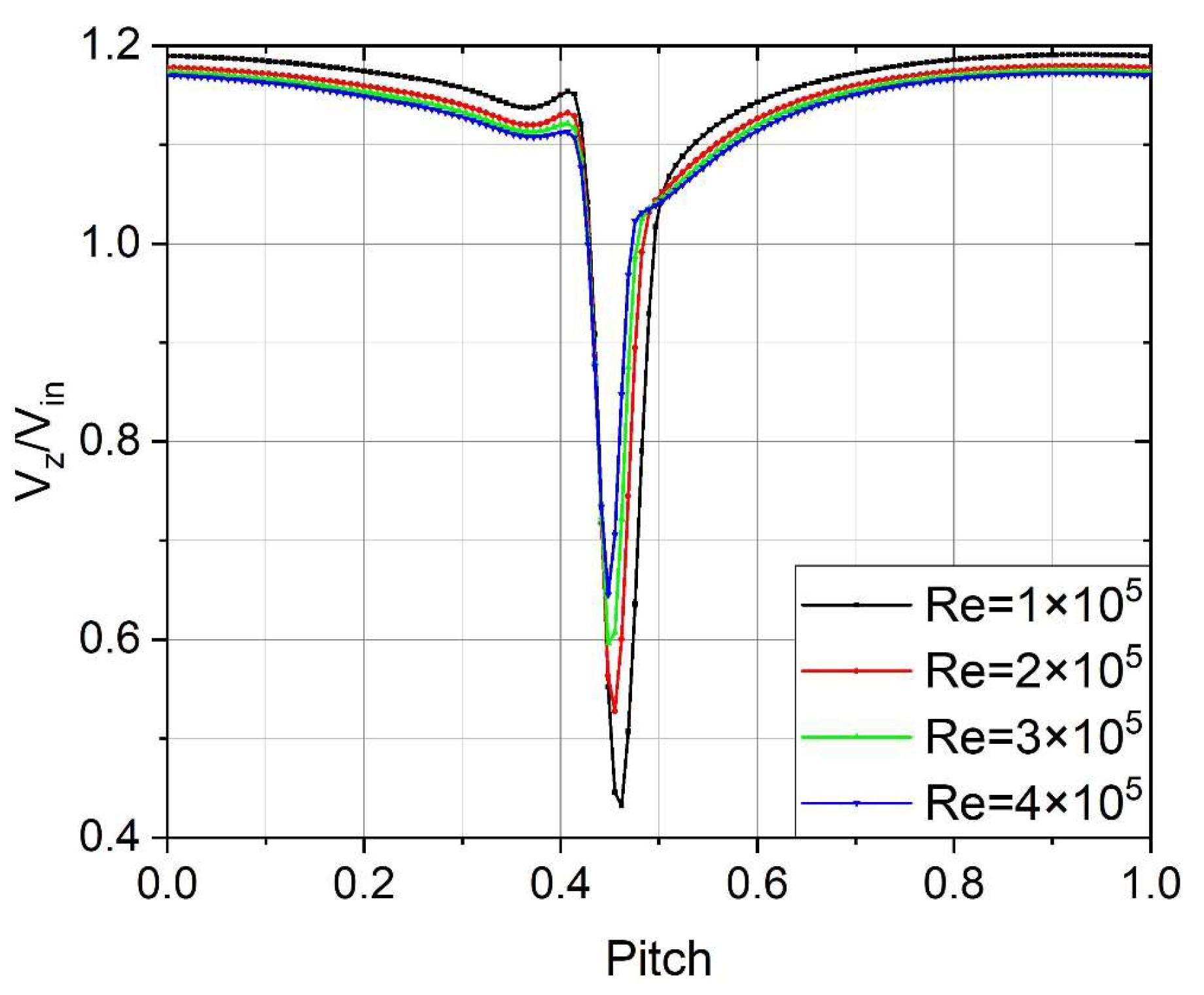
3.1. Effect of Wake on Compressor Performance at Different Re

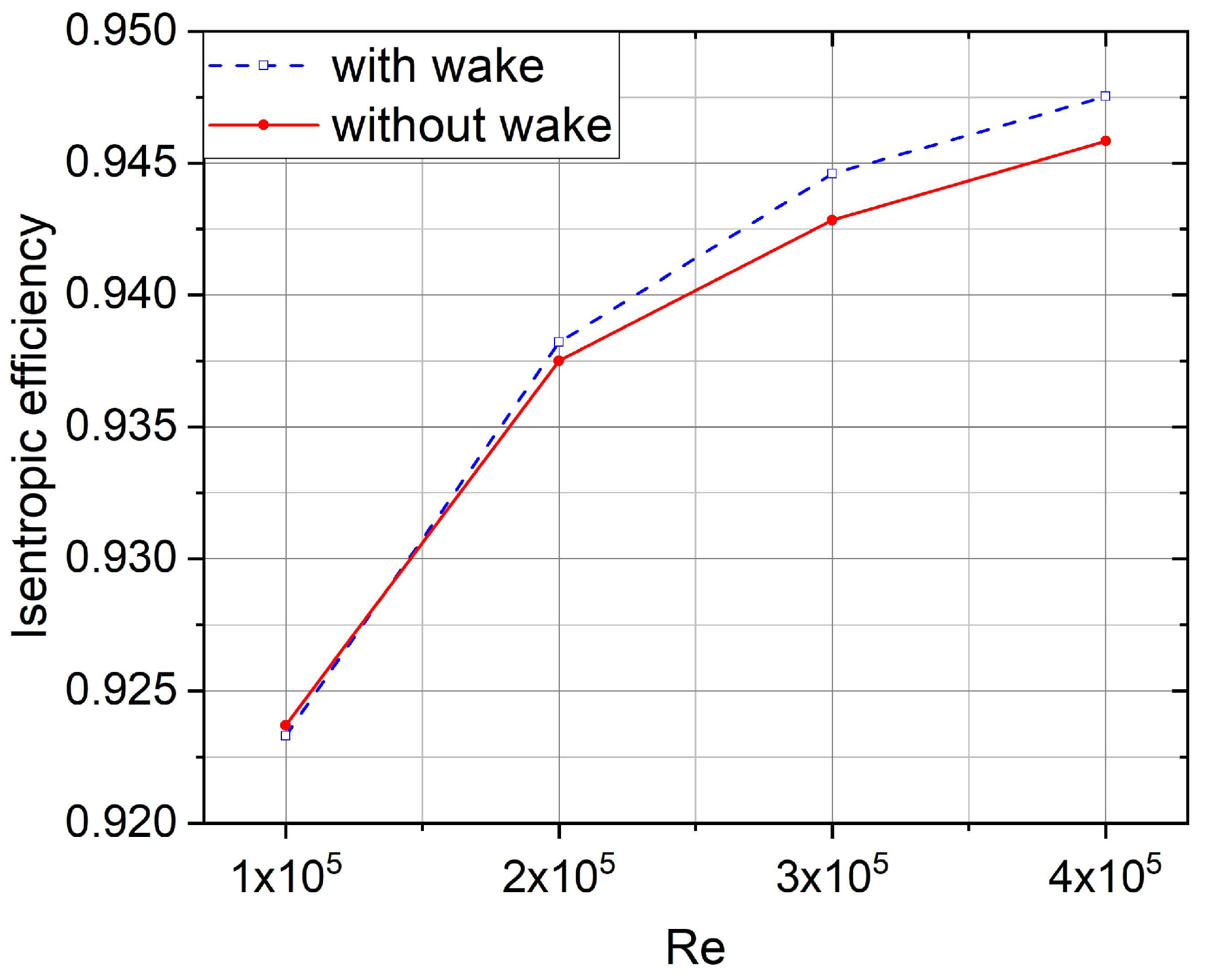
Eight cases with and without a wake were calculated at Re values from 1 × 10⁵ to 4 × 10⁵. The corrected mass flow and the corrected rotating speed of different cases remained the same. Because unsteady numerical simulations were used in the cases with the wake, many related results presented here have been time averaged. Based on Equation (1), the isentropic efficiency of the rotor with and without the wake at different Re is shown in Figure 6. Clearly, both the Re value and wake influence the rotor efficiency. The rotor is less efficient and the efficiency declines sharply at lower Re, which indicates that the Re effect is significantly enhanced at low Re, resulting in a large change in the flow characteristics and performance of the compressor. By comparing the operating conditions with and without wake, it can be seen that the change of Re will make the impact of wake on performance different. The unsteady wake has a beneficial effect on the efficiency of the rotor at Re = 4 × 10⁵, but this effect weakens as Re decreases until the effect is negative.
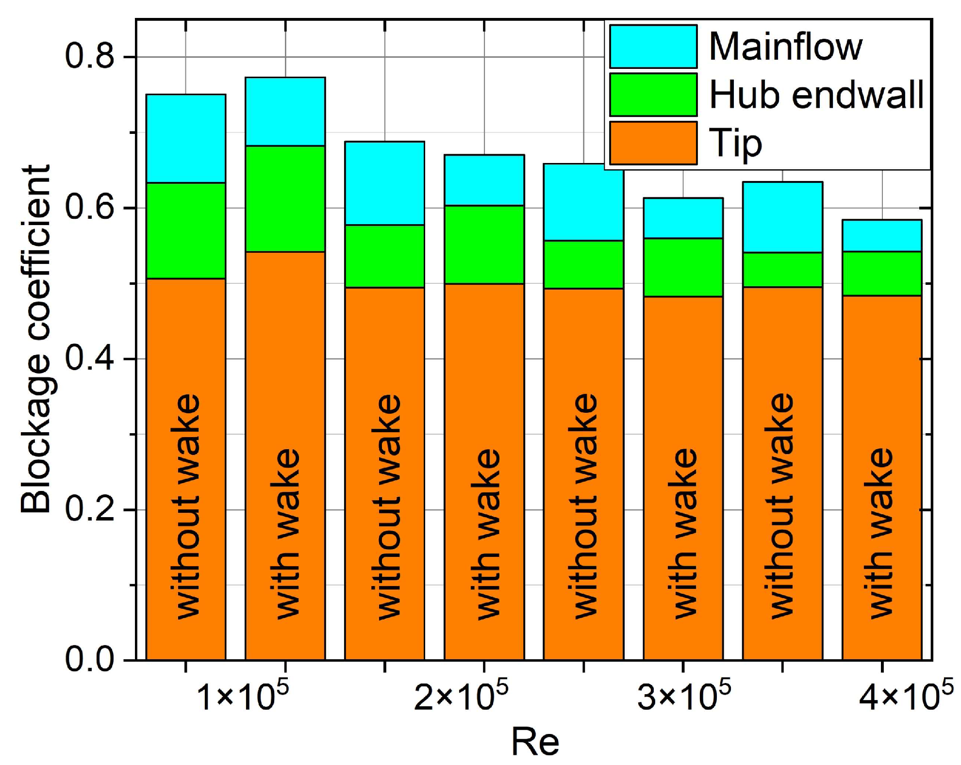
To quantitatively analyze the flow loss in different regions, the blockage coefficient of 10% chord length section after the rotor under different conditions is shown in Figure 7. The blockage coefficient is defined by Yu et al. [37] as
B m = m b m t = ρ A   V ext V dA m t
where mb and mt are respectively the reduced mass flow due to the flow blockage and the actual total mass flow; V is the streamwise velocity; Vext is the average streamwise velocity at the boundary of the blockage region; A is the total area of the blockage region. According to Equation (2), the key to obtaining the blockage coefficient is to determine the blockage region. Khalid et al. [38] proposed a method to identify blockage regions based on velocity density flow gradient, which is defined as
ρ V r ,   θ   = ( r ρ V ) 2 + ( θ ρ V ) 2 constant
where V is the streamwise velocity, and r and θ are respectively the radial direction and circumferential direction. Through the test, the blockage is not sensitive to the change of the constant, and the constant is chosen as 100. The blockage region of the rotor outlet is divided into three parts by radius. The blockage coefficient of all regions decreases with increasing Re, which is consistent with the change in rotor efficiency. The flow blockage in the tip region is dominant for all cases. For the cases without wake, although the flow blockage coefficient of the hub endwall region increases rapidly with the decrease of Re, it is still weaker than that of the tip and mainflow regions. However, the flow blockage coefficient of the mainflow region is lower than that of the hub endwall region for the cases with the wake. In the mainflow and hub endwall regions, the wake has the opposite impact. The unsteady effect of the wake can reduce the flow blockage caused by the blade in the mainflow region but increase the flow blockage caused by the hub boundary layer in the hub endwall region. In addition, the effect of the wake on the blockage coefficient of the tip region will change under different Re. The flow blockage is most severe in the tip region, and it is weakened by the wake only at the Re of 1 × 10⁵ and 2 × 10⁵. The difference in variation trend is mainly caused by the difference of flow characteristics at different Re.
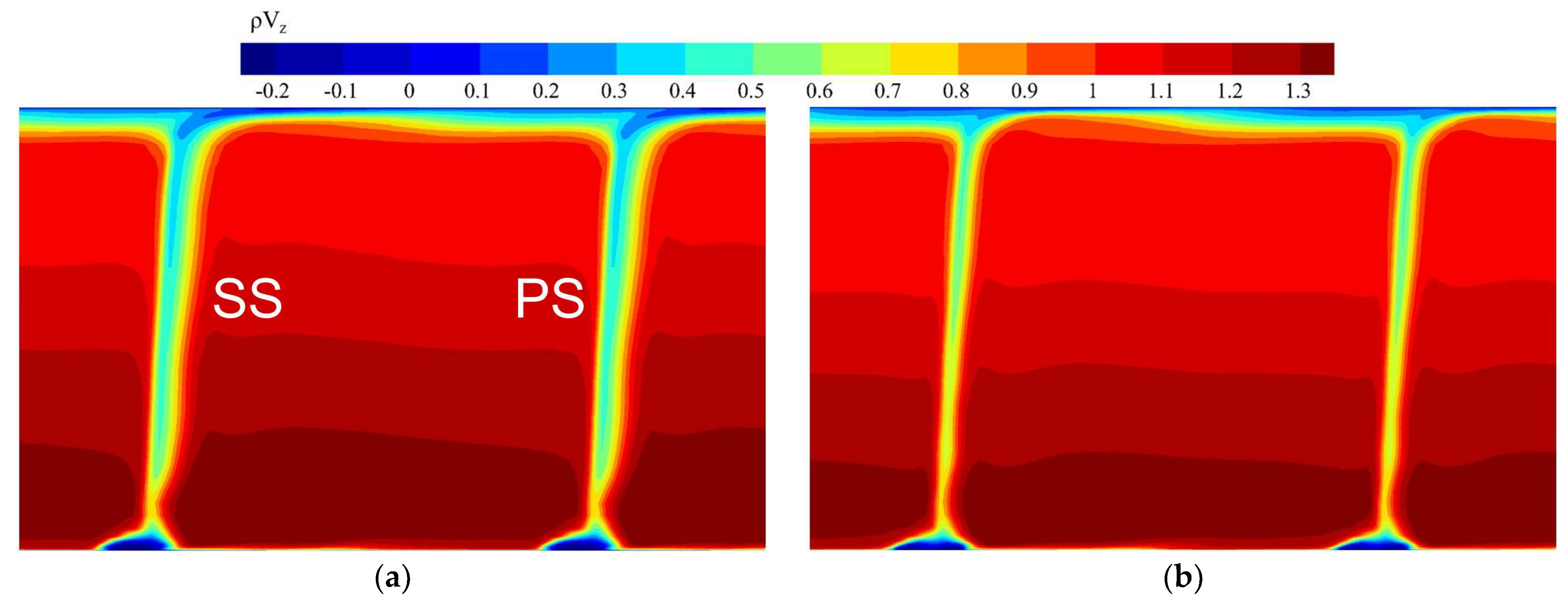
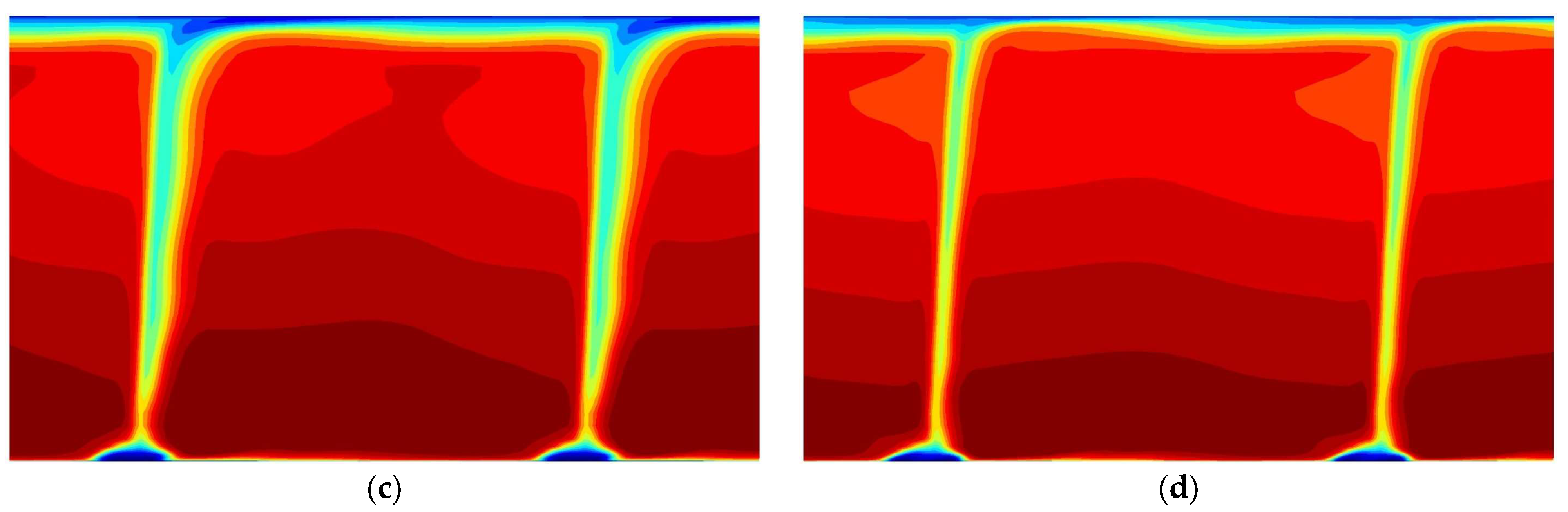
As shown in Figure 8, the axial velocity density flow of 10% chord length section after the rotor at the Re of 1 × 10⁵ and 4 × 10⁵ is compared to analyze the distribution of flow blockage in detail. As mentioned above, three blocked regions can be distinguished by radius. The tip region is affected by the tip leakage flow, so there is an area of low-density flow in the whole pitchwise direction. In contrast, the range of flow blockage at the hub endwall is concentrated downstream of the blade hub due to the absence of hub clearance. In the mainflow region, the flow blockage is mainly caused by the low-velocity fluid in the wake. Comparing the density flow at different Re, the blockage and flow loss increase as Re decreases from 4 × 10⁵ to 1 × 10⁵ due to the increase of viscous dissipation. The influence of the wake is more obvious at the Re of 1 × 10⁵, which leads to the increase of flow blockage behind the tip clearance and the decrease of flow blockage behind the blade. The change in density flow with the influence of the wake is following that of the blockage coefficient in Figure 7, and the above phenomenon indicates that the flow structure of the blade boundary layer and tip leakage flow change obviously under the influence of the wake. In addition, because of the unsteady effect caused by the wake, there is some circumferential nonuniformity of density flow in the mainflow region. Considering the representativeness of the mid-span and the characteristics of the leakage flow at the blade tip, subsequent analysis will focus on these two blade heights.
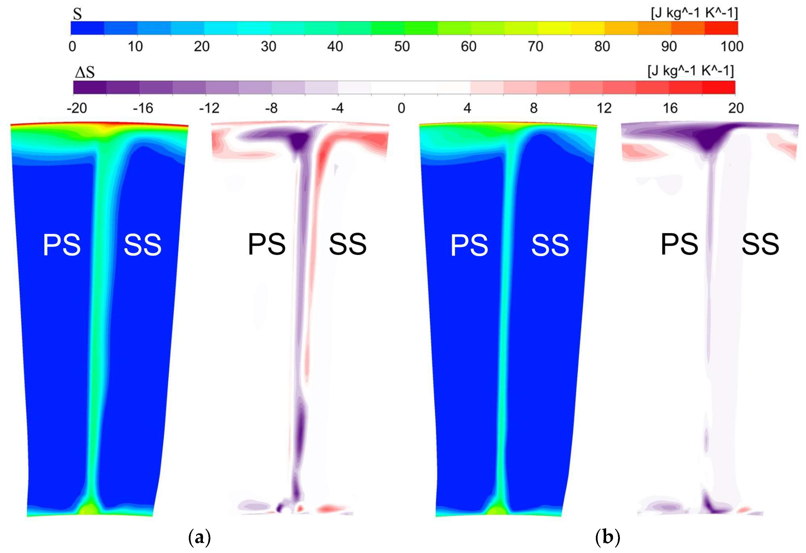
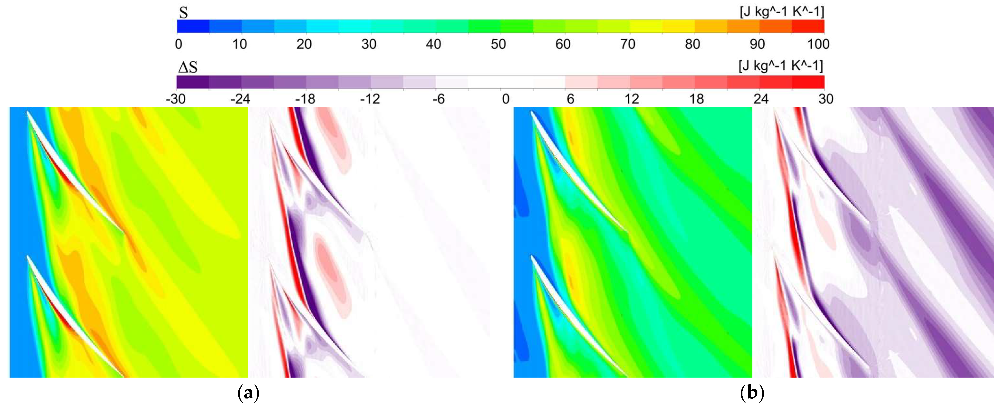
Figure 9 shows the static entropy distribution with wake of a 10% chord length section after the rotor. The static entropy can quantitatively reflect the flow loss in the compressor. The difference in static entropy is calculated by subtracting the case without the wake from that with the wake. The unsteady effect of the wake on the flow field can be directly determined from the contours of the difference between the URANS and RANS results. For all cases, a high-entropy region appears near the shroud and behind the blade, but the high-entropy region near the hub is small. At Re = 4 × 10⁵, the difference in entropy shows that the wake causes the entropy to decrease in the regions mentioned above, although there is an increase at the top of the mainflow region. Decreasing Re from 4 × 10⁵ to 1 × 10⁵ changes the contours of the entropy difference, except near the hub. The Re only affects the magnitude and range of the entropy reduction near the hub. With Re = 1 × 10⁵, the entropy behind the suction surface (SS) increases under the influence of the wake on the suction surface boundary layer. The magnitude and range of the entropy-reduction region behind the pressure surface (PS) increase, indicating the enhanced effect of the wake. Contrary to the conclusion at Re = 4 × 10⁵, the wake can increase the entropy near the shroud at Re = 1 × 10⁵.
According to the above analysis, it can be concluded that the unsteady effect of the wake has a more significant impact on the flow field at the tip and mid-span of the blade. The following sections analyze these two regions in turn.

3.2. Effect of Wake on the Mid-Span Flow Field at Different Re

The rotor section at 50% spanwise height is now investigated in detail to obtain the flow field information in the mainflow region. The circumferential distribution of inlet normalized axial velocity at different Re is shown in Figure 10. The axial velocity deficit represents the wake strength, and the wake becomes stronger and wider as Re decreases. Therefore, at low Re, the unsteady effects caused by a stronger wake are more obvious, and the influence on the downstream rotor characteristics is greater.
At low Re, the structure of the LSB keeps the pressure constant. As Re increases, the region of constant pressure decreases in size and has less influence on blade loading. The wake-induced boundary layer transition affects the size of the separation bubble, which is an important factor affecting the loading and performance of the rotor. 
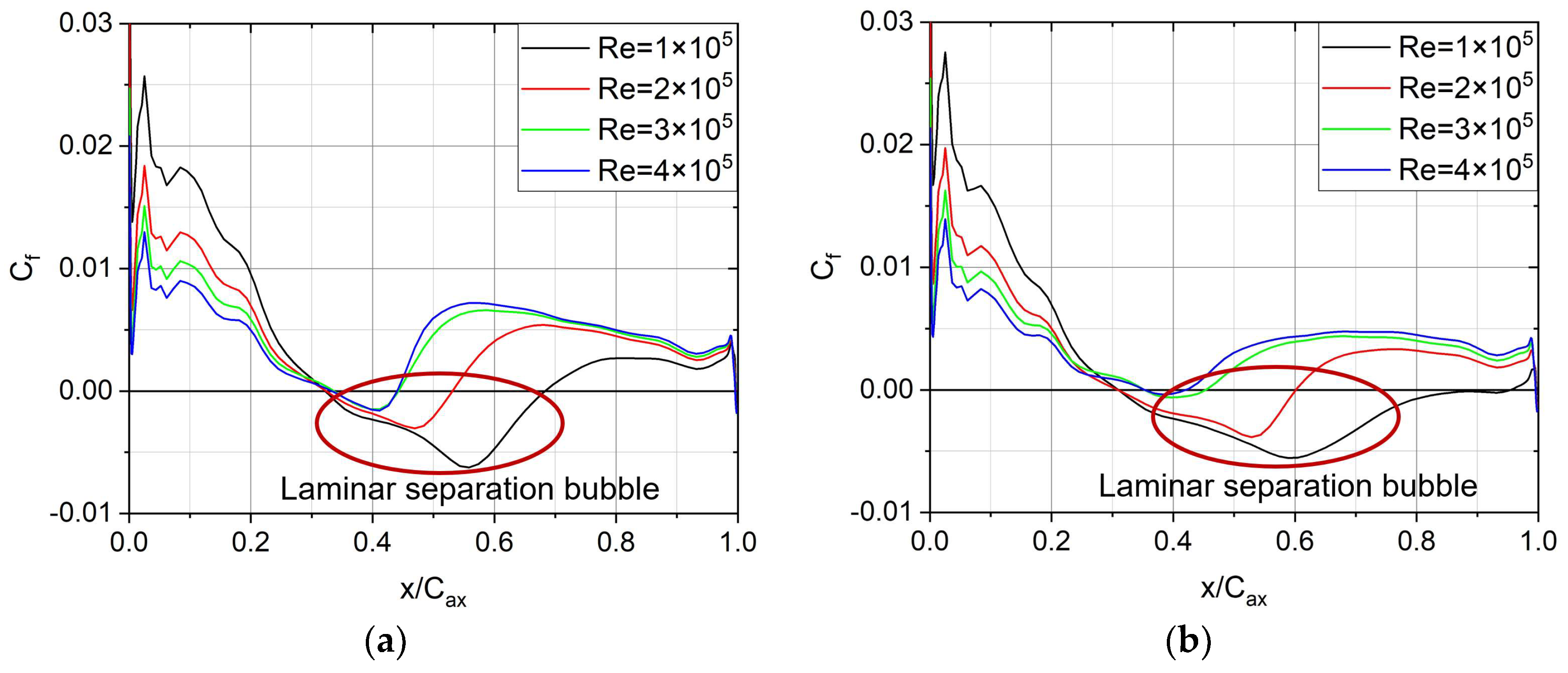
Figure 11 shows the skin friction coefficient (Cf) on the suction surface of the blade, from which the length of the LSB can be obtained. The positions at which Cf = 0 represent the points of separation and reattachment of the LSB. For the results with the wake, a decrease in Re causes the position of turbulent reattachment to move back and that of laminar separation to move forward. However, for the cases without the wake, the position of the boundary layer separation does not change with Re. By comparing the results with and without the wake, it can be concluded that the wake suppresses laminar separation and promotes turbulent reattachment at high Re but delays turbulent reattachment at low Re. Under the influence of wake, the length of the LSB increases at low Re and decreases at high Re. The flow loss caused by the LSB also changes with its length. The wake can input energy and disturbance to the boundary layer to affect its development. In addition, the process of wake-induced transition also indirectly affects the location of turbulent reattachment.
To analyze the detailed flow field within the boundary to obtain the boundary development process, Figure 12 shows the contours of the normalized mainflow velocity on the suction surface, where the dotted line indicates the displacement thickness of the boundary layer. The mainflow velocity is the velocity along the tangent line of the blade surface. In Figure 12, the horizontal axis x/Cax is the normalized length along the blade surface, and the vertical axis y/Cax is the normalized normal distance from the blade surface. The low-velocity region caused by the boundary separation can represent the position and size of the LSB. The low-velocity region increased significantly as the Re decreased from 4 × 10⁵ to 1 × 10⁵. The thickest position of the LSB is 0.5Cax, and the thickness of the LSB gradually decreased. The LSB in the case without wake disappears at 0.65Cax, but the wake can prevent the LSB from disappearing. In addition, the displacement thickness of the boundary layer thickens rapidly with the appearance of flow separation bubbles, which block the flow passage and increase the loss. In addition, the boundary layer develops into turbulent flow after reattachment, and the continuous increase in its thickness leads to a large loss due to turbulent viscosity dissipation. As Re decreases, the ability of the boundary to resist separation weakens, and the transition process is delayed, such that the length and thickness of the separation bubble increase. It is also clear that the thickness of the boundary layer increases with decreasing Re. Considering the influence of the wake, the boundary layer thickness decreases slightly at high Re and increases significantly to form an open separation bubble at low Re.
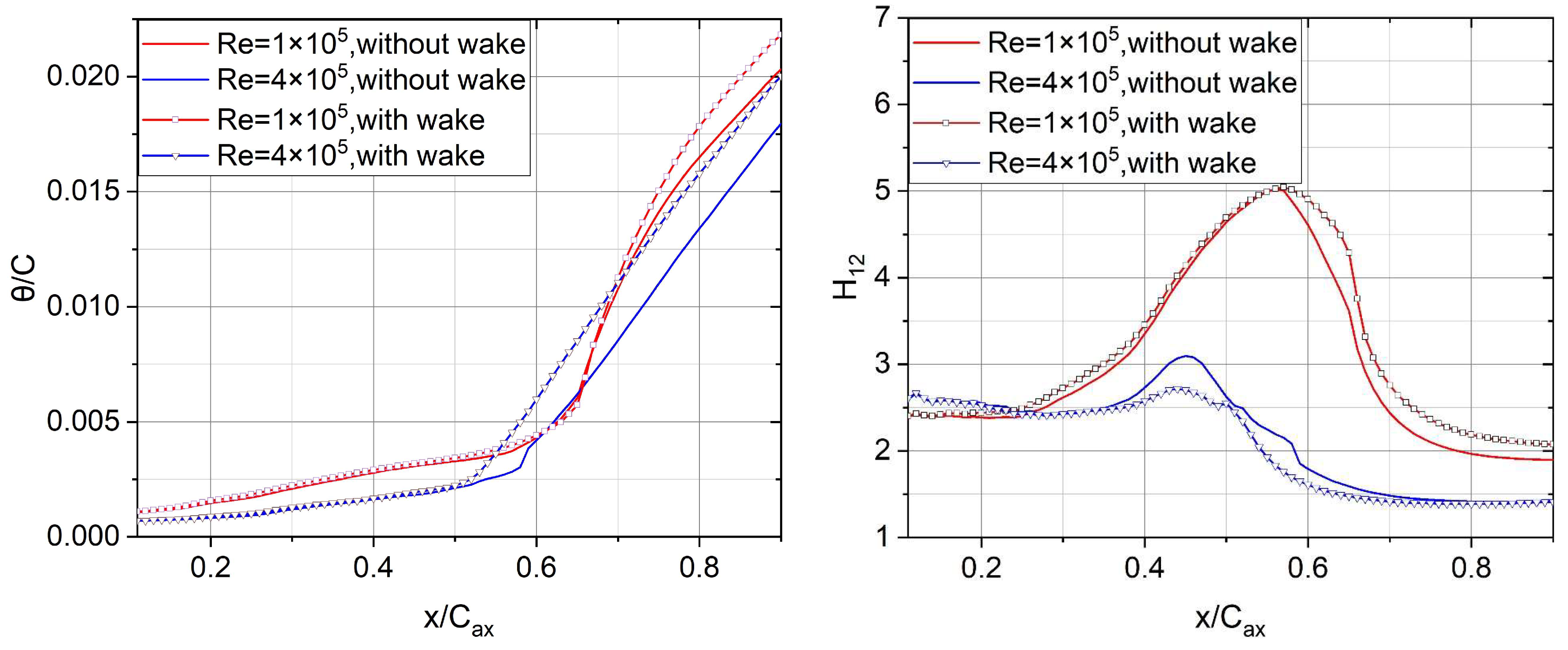
Figure 13 shows the distribution of suction surface boundary layer momentum thickness (θ) and shape factor (H12) at different Re. θ represents the magnitude of the loss of momentum caused by the viscous boundary layer. The turning point in the curve of θ indicates that the instability of the boundary layer is suddenly magnified, followed by a rapid increase in the loss of momentum. The reason for this phenomenon is the boundary layer transition, with the turning point representing the transition point. As Re decreases, the turning point of θ moves downstream and its growth rate increases after the turning point. A faster momentum thickness growth rate indicates stronger turbulent dissipation. The wake causes the turning point to move downstream at Re = 4 × 10⁵, but the wake no longer changes the turning point and only increases the growth rate of θ after the turning point at Re = 1 × 10⁵. H12 represents the velocity pattern of the boundary layer and reflects the separation and transition phenomena. A larger value of H12 indicates more obvious boundary layer separation at Re = 1 × 10⁵. By comparing H12 in the cases with and without the wake at Re = 1 × 10⁵, it is apparent that the position before the maximum thickness of the separation bubble is not affected by the wake. However, the wake can increase the separation size of the turbulent boundary layer after the transition. The difference in H12 is consistent with the changes in momentum thickness, and the region affected by the wake at Re = 1 × 10⁵ is the turbulent boundary layer after the transition. At Re = 4 × 10⁵, the change in momentum thickness indicates that the wake advances the boundary layer transition. Therefore, the ability of the boundary layer to resist separation is enhanced, and the size of the boundary layer separation is reduced. There is a significant decrease in H12 over the entire separation bubble region.
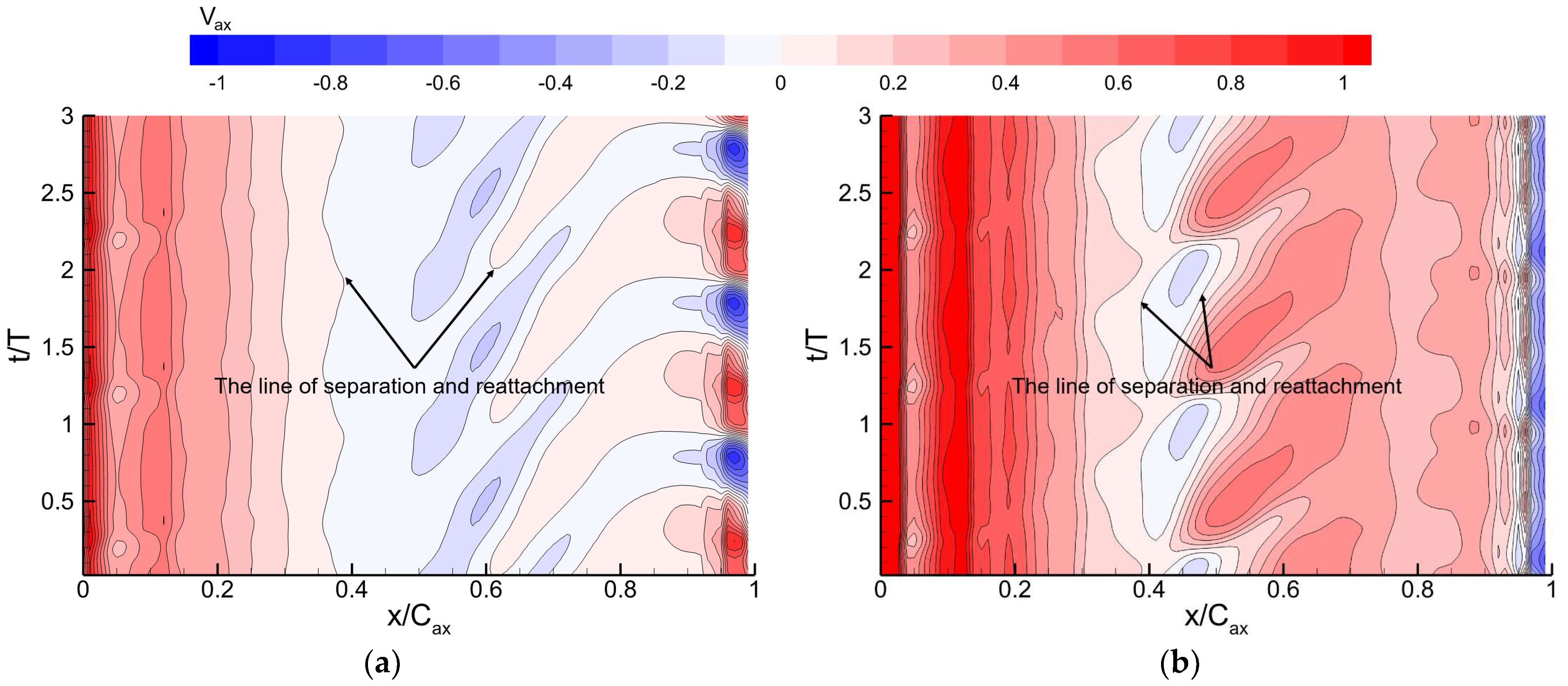
A series of time-dependent data are obtained by setting monitoring points along the line of the blade suction surface at 50% span. To explore the development of the boundary layer at the wall induced by the periodic wake, three passage periods of the rotor are selected and the phase-locked average results are calculated to obtain the space-time diagram on the suction surface at 50% span. The space-time diagram of the normalized axial velocity is shown in Figure 14. The axial velocity of the first mesh layer on the wall is used to represent the state of the boundary layer separation. As there is backflow in the LSB, the position at which the boundary layer starts to separate is represented by a near-wall velocity of zero, and the region with a negative near-wall velocity represents the boundary layer separation region. At Re = 4 × 10⁵, the boundary layer is disturbed by the wake, and the starting point of separation changes continually. At a certain time, the LSB appears, and the position of turbulent reattachment moves downstream. The starting position of separation then shifts downstream until the LSB has completely disappeared. At Re = 1 × 10⁵, the position of boundary layer separation fluctuates periodically under the wake effects. The sweep of the wake also causes the LSB to fall off at the tail and then move downstream with the wake. When the detached separation bubble moves to the trailing edge of the rotor, its ability to resist separation is relatively weak. Therefore, a large region of turbulent separation forms at the trailing edge. At Re = 4 × 10⁵, the transition occurs closer to the leading edge of the blade, and the boundary layer flow is completely turbulent after reattachment. The turbulent separation is less affected by the wake and does not change with time. Instead, turbulent separation occurs periodically due to the effect of the wake at Re = 1 × 10⁵.
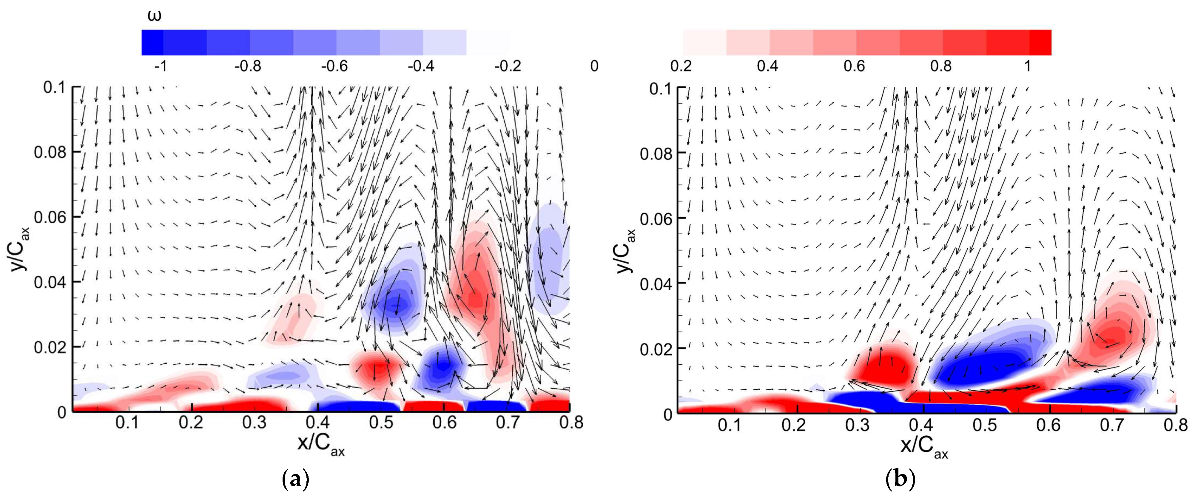
A vector diagram of the transient disturbance velocity and contours of the normalized transient disturbance vorticity at the same time are shown in Figure 15. There is a prominent reverse vortex downstream of the wake, which slows the flow of the boundary layer and generates small-scale vortices that affect the boundary layer. Forward and reverse vortices appear alternately, which accelerate and decelerate the boundary layer flow, respectively. 
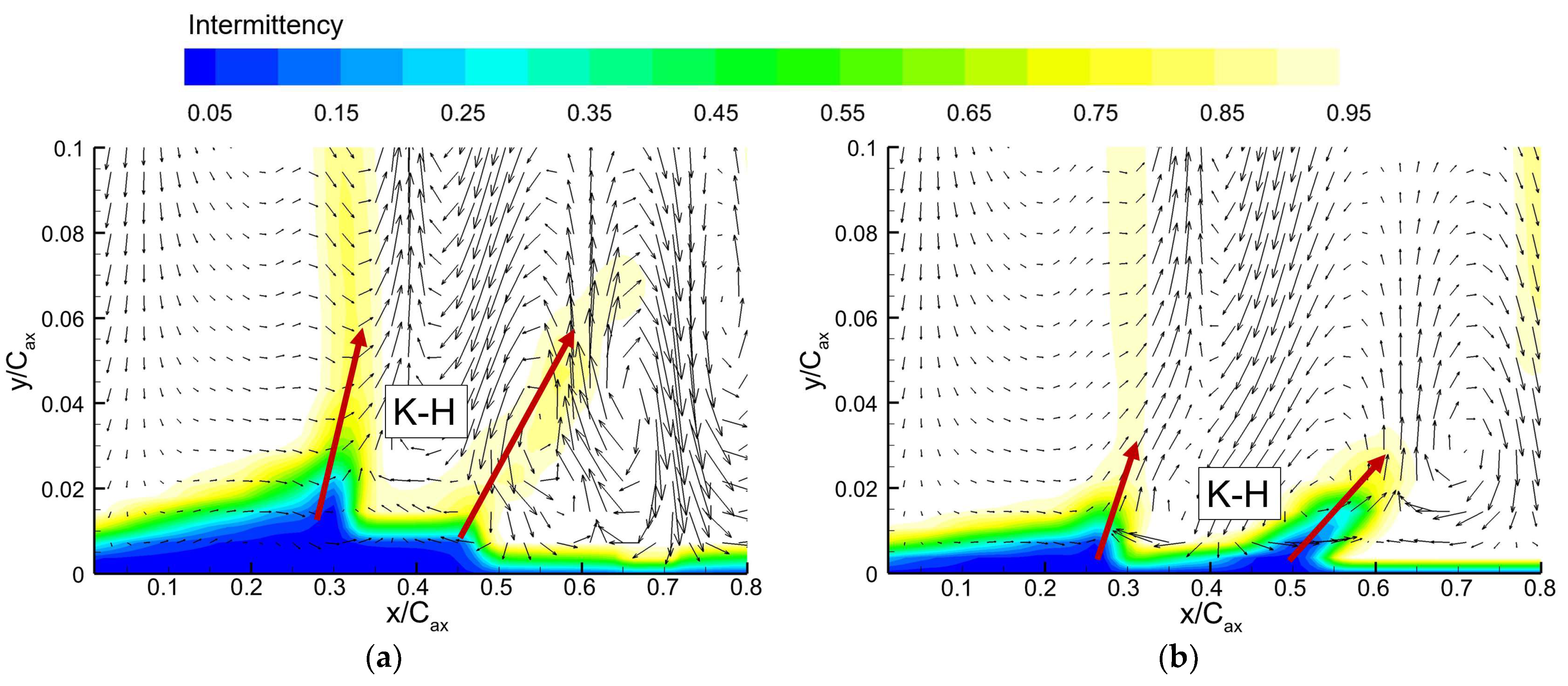
Figure 16 shows the transient intermittency contours at the same time to indicate the flow status. Intermittency values of 0 and 1 represent fully laminar flow and fully turbulent flow, respectively. The transition process is caused by the instability of the boundary layer. There are two main types of viscous instability: Tollmien–Schlichting and inviscid K-H. The main phenomena of the transition caused by the K-H instability are vortex rolling, shedding, pairing, and crushing, resulting in a strong mixing and momentum exchange between the boundary layer and the mainflow region. In general, the dominant instability type is affected by the boundary thickness, and the separation boundary layer mainly exhibits K-H instability. At the position of the separation bubble, the region where the intermittency factor changes significantly near the mainflow region is caused by the K-H instability. With boundary layer reattachment, the K-H instability disappears. The K-H instability induced by the wake dominates the transition process in the separated shear layer.
Figure 15 and Figure 16 indicate that the reverse vortex moves upstream with decreasing Re, leading to an expansion of the region of influence of the wake and the induced transition region. The vortex intensity is relatively weak, and the derived vortex has a smaller influence range at low Re. However, the number of derived vortexes is greater than that at high Re. In the case of high Re, the area of vortex concentration is closer to the blade due to the thicker boundary layer. Compared with the result at Re = 1 × 10⁵, the K-H instability induced by the wake develops more rapidly at Re = 4 × 10⁵ due to the higher vortex intensity. As the wake moves downstream, the transition process caused by the K-H instability accelerates under Re = 1 × 10⁵. Therefore, the region of transition near the blade trailing edge decreases significantly. With Re = 4 × 10⁵, the K-H instability is weakened by the reattachment of the LSB. Therefore, the transition process decelerates, and the transition region near the blade trailing edge becomes larger.

3.3. Effect of Wake on the Tip Flow Field at Different Re

According to the analysis in Section 3.1, the upstream wake and TCV have strong unsteady effects, which in turn influence the compressor performance. The unsteady interaction varies with Re. The contours of the static entropy with wake and its difference with no wake at 99% span are shown in Figure 17, illustrating the influence of the wake on the flow loss of the tip flow field. The calculation method of the difference in entropy is consistent with Figure 9. For the result with the wake at Re = 4 × 10⁵, the high-entropy region is concentrated in the region influenced by the TCV and develops from the suction side leading edge across the flow passage to the pressure surface of the adjacent blade. According to the difference in entropy at Re = 4 × 10⁵, there is a strip in which the entropy is increased by the interaction in front of the TCV. Although the direct mixing effect caused by the wake rapidly increases the entropy, the unsteadiness of the wake changes the TCV intensity by influencing the blade loading, resulting in a reduction in flow loss because of boundary layer separation at the trailing edge. As the entropy reduction outweighs the entropy increase, the flow blockage becomes weaker at the tip region. In the case of a wake with Re = 1 × 10⁵, the high-entropy region has a greater range over the whole flow passage, except at the inlet, indicating that the flow loss caused by the TCV increases sharply at low Re. As Re decreases from 4 × 10⁵ to 1 × 10⁵, the entropy difference shows that the mixing loss caused by the wake and TCV remains almost unchanged, but the range of entropy reduction in the TCV core region becomes larger. The magnitude and range of the entropy reduction behind the blade decrease significantly, indicating that the beneficial effect of the wake on the flow loss has decreased. In addition, there is a region in which the entropy increases in the center of the flow passage. This is because the intensity of the double-leakage flow increases under the influence of the unsteadiness at Re = 1 × 10⁵.
The strength of the TCV is affected by the tip loading distribution. To determine the strength and position of the TCV under the influence of the wake, Figure 18 shows the distribution of the static pressure coefficient at 99% span and the mass flow rate of the tip leakage flow distribution at different Re. The mass flow rate distribution of the tip leakage flow is the axial distribution of the average velocity times density along the tip clearance height. The compressor blade is a front-loading type, so the maximum loading position is located at the leading edge. The large leakage flow region ranges from 10% to 30% of the axial position and corresponds to the high-loading region. Due to the large incidence, the pressure coefficient of the pressure surface drops sharply at the leading edge and then gradually increases until the 20% axial position. After the turning point, the increase in the pressure coefficient on the pressure surface slows down; this position is the same as the maximum leakage flow position. The leakage flow fluctuates before the 50% axial position, mainly because of fluctuations in the loading on the suction surface. After the 50% axial position, the static pressure coefficient of the suction and pressure surfaces starts to rise steadily, and the leakage flow exhibits a corresponding steady decline. Comparing the calculation results at different Re, we find that the pressure coefficient on the pressure surface decreases slightly with decreasing Re. The pressure coefficient on the suction surface increases slightly at the front part of the blade and decreases slightly at the back. The change in the loading distribution leads to a decrease in the tip leakage flow at the front of the blade and an increase at the back at Re = 1 × 10⁵.
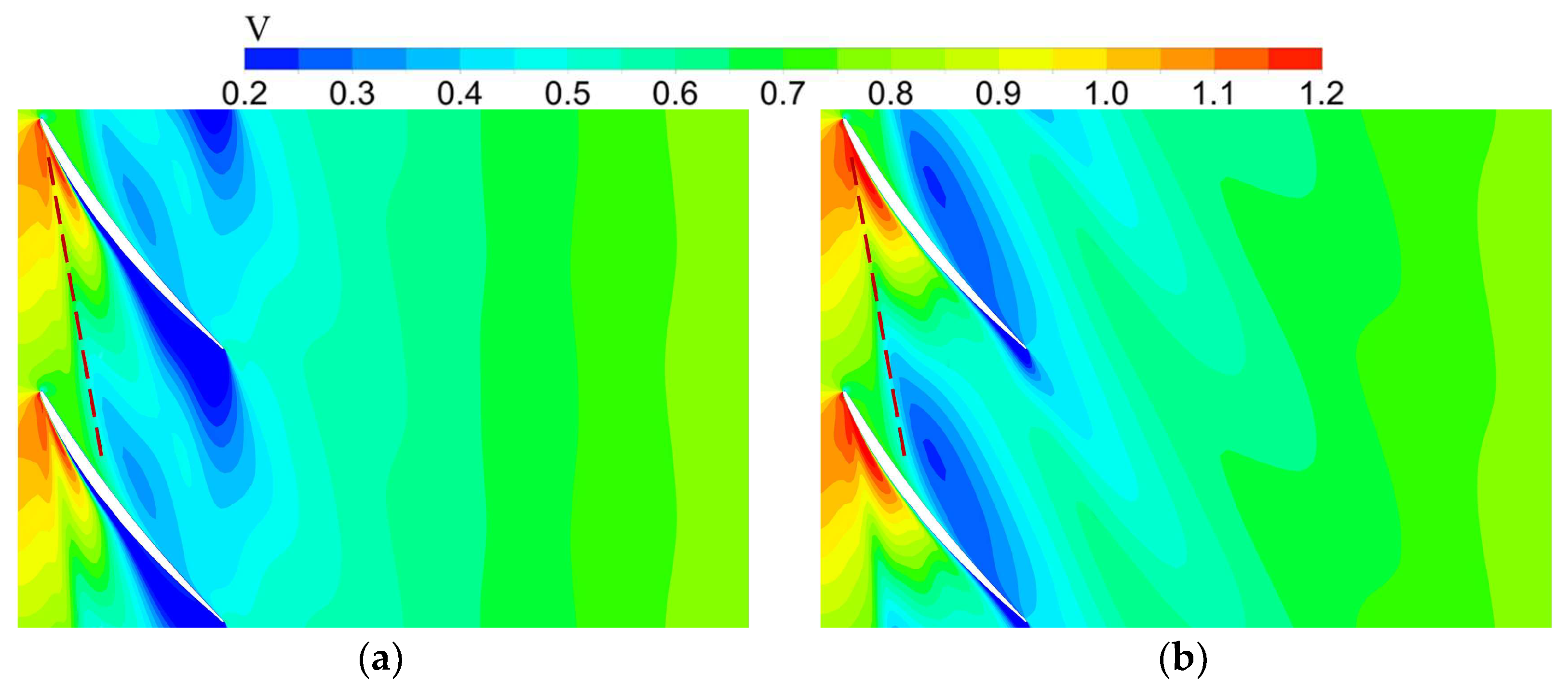
Figure 19 shows the time-averaged relative velocity contours at 99% span, with the average relative velocity of the rotor inlet adopted for normalization. The velocity of the TCV is lower than the mainflow velocity, resulting in a large low-velocity region and flow blockage in the tip flow field. As the TCV causes a sharp decline in the velocity of the mainflow, an obvious dividing line (dashed line in Figure 19) occurs at its front, and there is a large velocity gradient along this dividing line. Comparing cases at different Re, we see that the TCV intensity at low Re is relatively weak, and the range of the low-velocity region diffusing to the trailing edge of the adjacent blades’ pressure surface is smaller. When the TCV diffuses to the trailing edge region of the adjacent blades’ pressure surface, a double-leakage flow is generated at the blade tip. The double-leakage flow crosses the tip clearance, interacts with the suction surface boundary layer, and mixes with the wake caused by the separation of the rotor boundary layer. It can also be seen that the low-velocity region generated by the interaction between the double-leakage flow and the rotor boundary layer is significantly affected by the Re, and the range of the low-velocity region increases significantly at Re = 4 × 10⁵. The reason is that the ability of the fluid to resist separation is weak at low Re. Although the strength of the TCV is weak, the slight disturbance of the double-leakage flow still leads to boundary layer separation over a significant range and a large low-velocity region. For Re = 4 × 10⁵, the interaction between the double-leakage flow and the boundary layer at the trailing edge of the rotor is weak, so its effect on the flow field is not obvious, and only a small low-velocity region is generated.
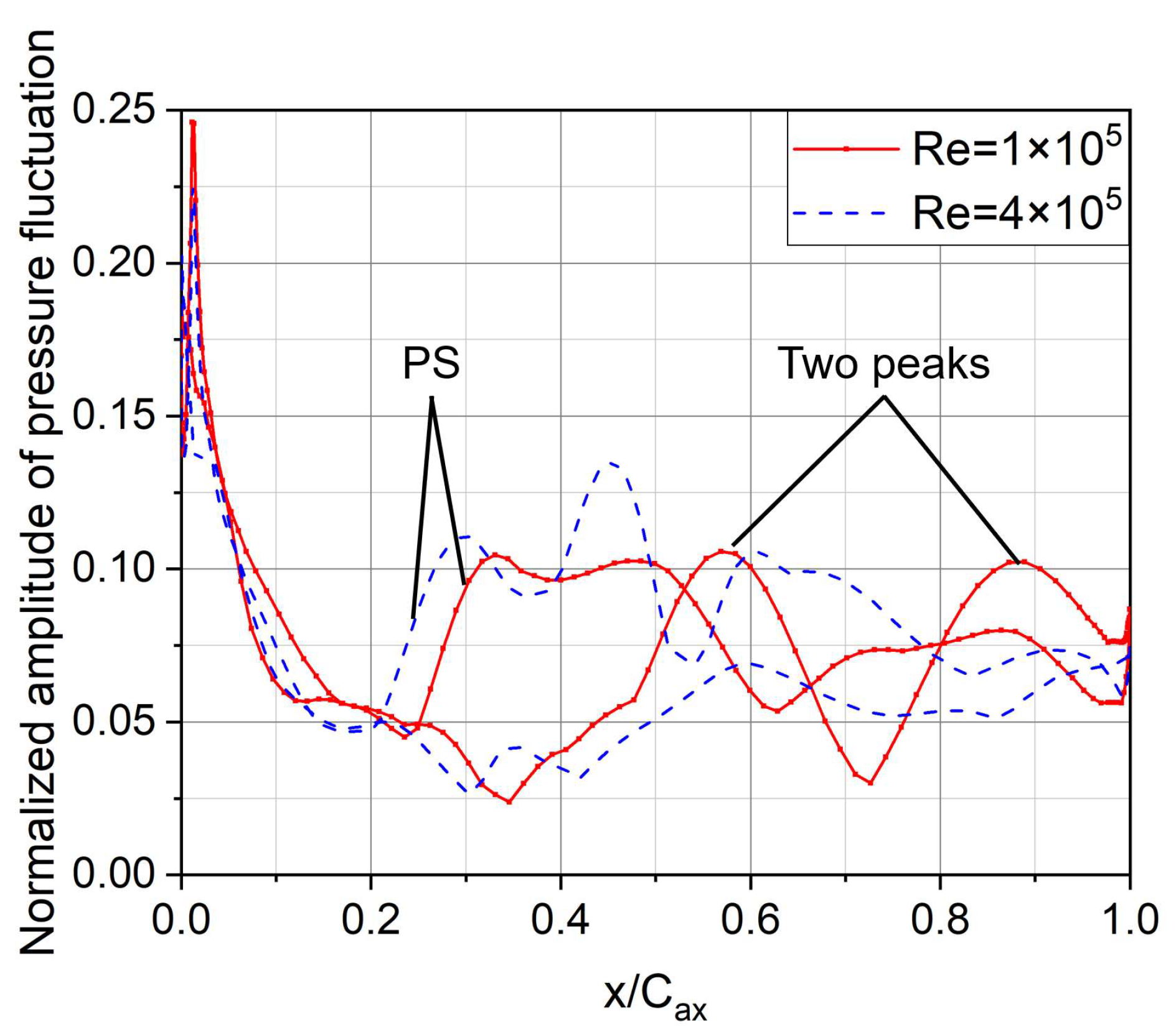
The TCV interacts with the upstream wake in the development process. As shown in Figure 20, the amplitude of pressure fluctuations on the rotor surface at 99% span is selected for comparison. The difference between the maximum and minimum pressure at different times gives the amplitude, with the average static pressure at the rotor inlet used for normalization. The amplitude of pressure fluctuations at the leading edge of the pressure surface is large because of the influence of the incoming flow wake and TCV, and then gradually decreases until the 25% axial position. As the TCV reaches the pressure surface across the flow passage, the amplitude of the pressure surface fluctuation increases again due to the strong disturbance of the TCV. The leading edge of the suction surface exhibits similar behavior to the pressure surface, and the amplitude of pressure fluctuations decreases until the 35% axial position. The amplitude on the suction surface exhibits different trends at different Re. For the low Re condition, the double-leakage flow and boundary layer separation produce two local peaks in the fluctuation amplitude on the suction surface, and these peaks are significantly larger than the fluctuation amplitude at Re = 4 × 10⁵. However, at Re = 4 × 10⁵, the fluctuation amplitude on the suction surface only increases slightly under the influence of the double-leakage flow. The pressure fluctuation amplitude on the pressure surface is more obviously affected by the TCV at Re = 4 × 10⁵, which is larger than that of the suction surface and is greater than the pressure fluctuation amplitude at Re = 1 × 10⁵. In conclusion, the pressure unsteadiness is mainly caused by the wake, TCV, and double-leakage flow at low Re, which are mainly located at the leading edge, 30–50% axial position of the pressure surface, and 50–100% axial position of the suction surface.
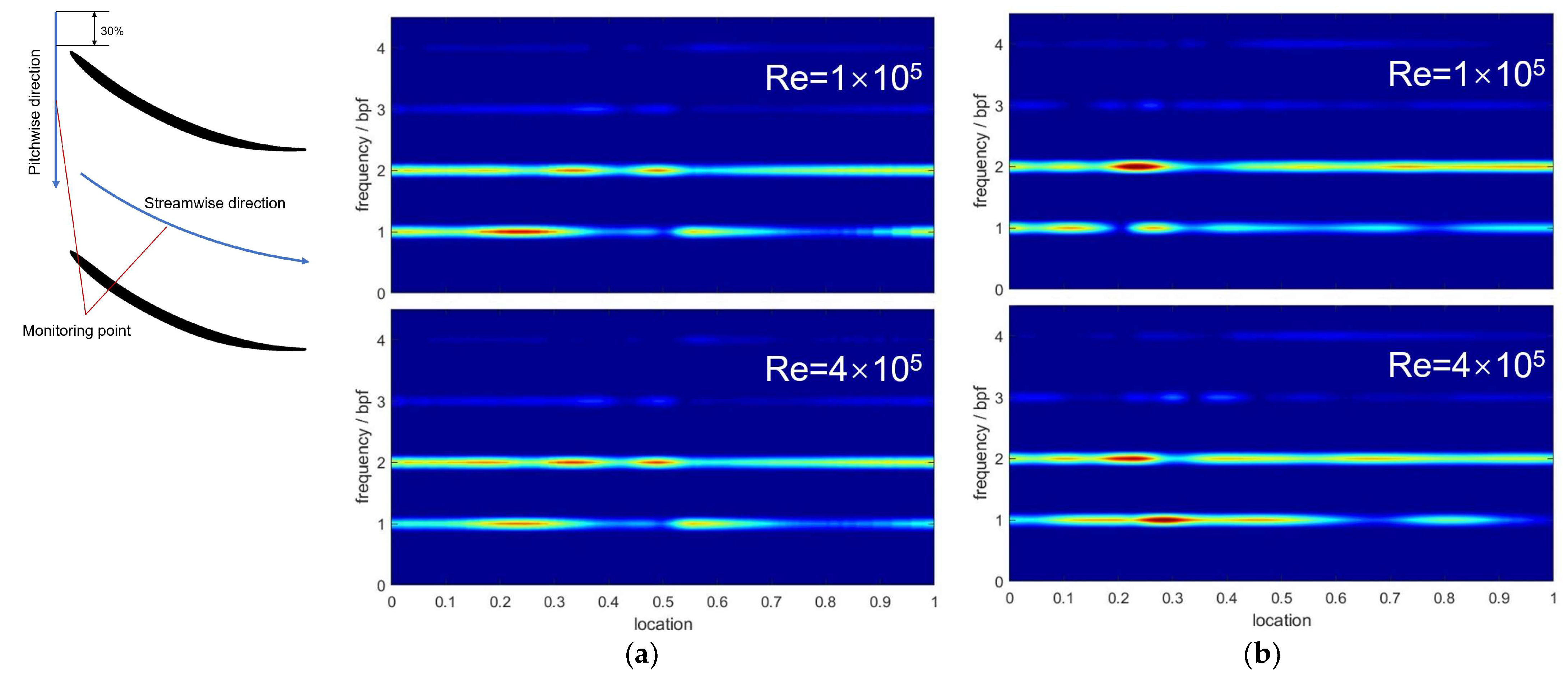
To quantify the unsteady pressure fluctuation in the tip flow field induced by the wake, the pressure signal from the time domain is converted into the frequency domain via fast Fourier transform (FFT). As shown in Figure 21, the monitoring points used for FFT are extracted along the streamwise direction inside the rotor and along the pitchwise direction at the rotor inlet. Figure 21 shows the amplitude-frequency characteristics of the monitoring points at 99% span. For the unsteady perturbation in the tip region, blade passage frequency (BPF) and 2BPF are dominant, while the amplitude of 3BPF and 4BPF is relatively small. Along the pitchwise direction at the rotor inlet, the influence range of 2BPF is the largest. Due to the interaction between the TCV at the leading edge and the wake, three regions with a large amplitude of 2BPF and one region with a large amplitude of BPF are located near the blade. There is also a large amplitude region of BPF at 0.5 to 0.7 normalized pitchwise length, but this region does not change at different Re. With the Re decreasing from 4 × 10⁵ to 1 × 10⁵, only the amplitude of BPF near the blade increases slightly. Along the streamwise direction, the amplitude of BPF and 2BPF increases rapidly, which is induced by the rapid development of the unsteady tip leakage flow. Subsequently, the influence of BPF weakens, while 2BPF is still dominant in the flow field. Comparing the results of different Re, it is found that the influence range and amplitude of 1BPF are larger at high Re.
In general, there are two kinds of interaction between the wake and TCV. First, the wake of the IGV generates a negative jet disturbance, which directly interacts with the TCV in the tip region, resulting in strong unsteady effects. Second, the wake periodically changes the loading distribution, thus indirectly affecting the strength and position of the TCV.
Figure 22, Figure 23 and Figure 24 show characteristics of the transient flow field at the same time under different Re conditions. The normalized relative velocity, normalized radial vorticity, and root mean square of the normalized axial velocity disturbance are selected for comparison. These flow parameters distinguish the mainflow and secondary flow phenomena, such as the wake and TCV, allowing their interaction mechanism in the flow field to be identified. The normalized radial vorticity is defined as
ω r = ω 0 C ax V in
where ω0 is the radial vorticity, Cax is the axial chord length of the blade, and Vin is the time-averaged relative velocity at the rotor inlet. The other two velocity parameters are normalized by Vin. The transient relative velocity contours are shown in 
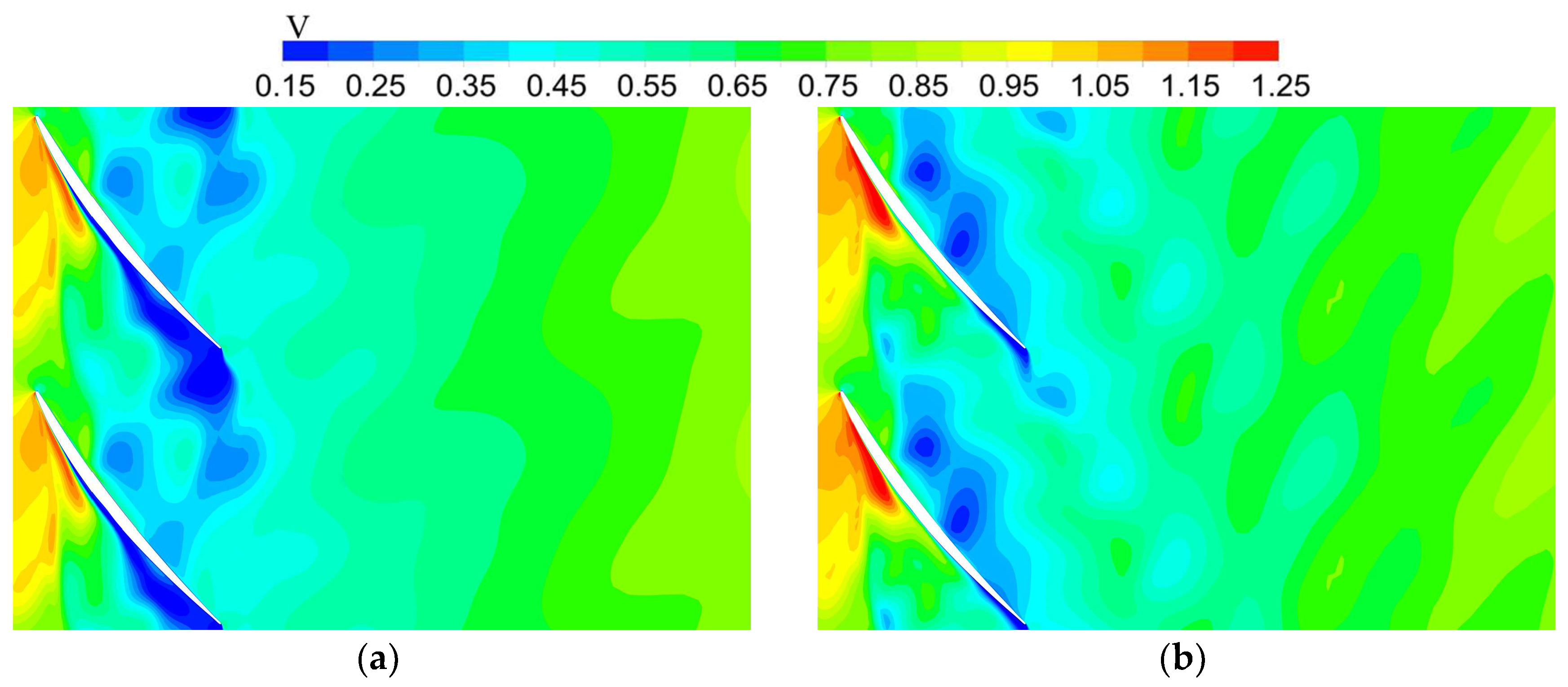
Figure 22, where the TCV is divided into multiple low-velocity regions. As Re decreases, the range of each low-velocity region becomes smaller. At Re = 1 × 10⁵, the unsteady interaction between the double-leakage flow and the suction surface boundary layer causes a wide low-velocity region to appear near the trailing edge. This region also presents multiple parts, causes a large flow blockage, and directly contacts the TCV on the pressure surface, which makes the tip flow field deteriorate sharply. In addition, the low-velocity region changes the shape of the rotor wake. The wake of the rotor no longer propagates downstream, and the low-velocity region caused by boundary layer separation and the double-leakage flow cover the whole outlet. However, the double-leakage flow only affects a small part of the trailing edge at Re = 4 × 10⁵, resulting in a low-velocity region. This region mixes with the rotor wake and flows downstream.
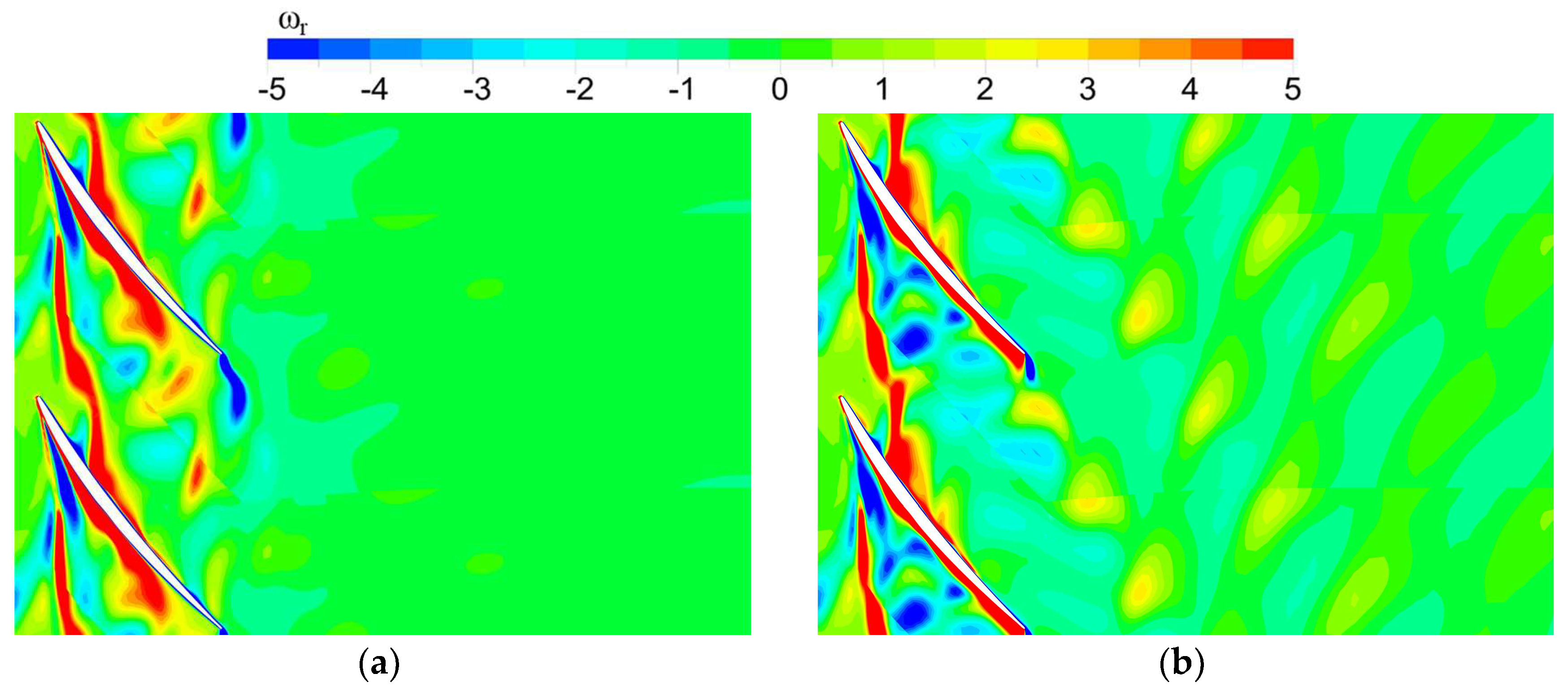
Figure 23 shows the radial vorticity contours, which can indicate the position of the interaction between the wake and TCV. The negative vorticity introduced by the wake is truncated by the tip leakage flow. At Re = 4 × 10⁵, the wake propagation path changes after it passes through the TCV. Subsequently, the wake continues to influence the flow field behind the TCV, which inhibits the action of the double-leakage flow and hinders the development of the boundary layer separation. At Re = 1 × 10⁵, the wake dissipates and mixes with the TCV. The dissipation of the wake caused the amplitude of 1BPF at Re = 1 × 10⁵ to be smaller than that at Re = 4 × 10⁵, as shown in Figure 21. The influence of the wake after the TCV is greatly weakened, and the double-leakage flow becomes the dominant factor controlling the flow field. In addition, although the rotor wake vortex is stronger at low Re, it stops propagating downstream due to the interaction with the boundary layer separation. Therefore, there is no interaction between the IGV wake and the rotor wake downstream of the rotor. 
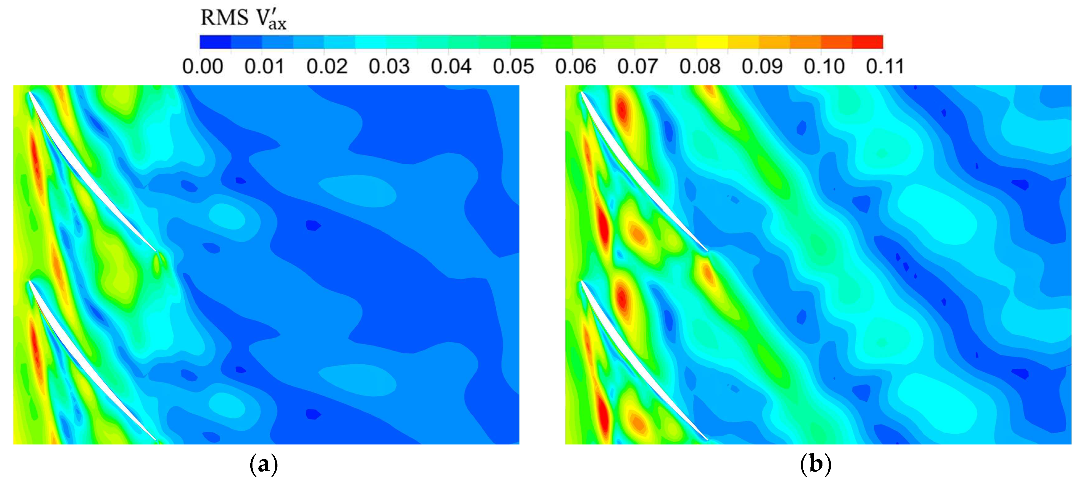
Figure 24 shows the root mean square of the axial velocity disturbance, representing the intensity of unsteadiness caused by the TCV and wake. The wake region and TCV region are the main fluctuation regions in the blade tip flow field, but the interaction between the wake and TCV varies with the Re value. There are two disturbance core regions at Re = 1 × 10⁵, while there are three disturbance core regions at Re = 4 × 10⁵. The difference is mainly caused by variations in TCV strength and loading distribution. At Re = 4 × 10⁵, the wake passes through the TCV and interacts with it strongly, resulting in an obvious disturbance region downstream of the TCV. However, the large suction surface separation caused by the interaction between the double-leakage flow and boundary layer at Re = 1 × 10⁵ is an important factor in the flow field disturbance.

4. Conclusions

The effect of an unsteady wake on the downstream flow field in a high-pressure compressor has been investigated in detail. The differences in the flow field with and without the wake were obtained by comparing the steady and unsteady calculation results. In addition, the influence of the Reynolds number on the wake unsteadiness was considered. The main conclusions can be summarized as follows.
The wake was observed to have a beneficial effect on the efficiency of the rotor at a high Reynolds number, but this effect weakened and became negative with decreasing the Reynolds number. The blockage region of the rotor outlet was divided into three parts: tip region, mainflow region, and hub endwall region. The flow blockage in the tip region was found to be mainly caused by the tip clearance vortex, which is the dominant factor in the loss over the whole flow field. The wake produced a different effect on the flow blockage in the tip region at different Reynolds numbers, consistent with the trend in efficiency. Compared with the static entropy of the outlet without the wake, the presence of the wake increased the entropy at the top of the mainflow region. As the Reynolds number decreased from 4 × 10⁵ to 1 × 10⁵, the magnitude and range of the entropy reduction region behind the blade pressure surface increased. Due to the influence of the wake on the blade suction surface boundary layer, the entropy behind the suction surface increased and combined with the top of the mainflow region at the Reynolds number of 1 × 10⁵.
For the flow field at 50% span, the laminar separation bubble was found to be an important structure of the suction surface boundary layer at a low Reynolds number, effectively changing the blade loading distribution and affecting the flow loss. As the Reynolds number increased, the size of the laminar separation bubble decreased. For the case without the wake, the position of laminar separation did not change with varying the Reynolds number. The wake caused the separation position to move forward and the reattachment position to move backward at a Reynolds number of 1 × 10⁵ and 2 × 10⁵. The opposite effect was observed at a Reynolds number of 3 × 10⁵ and 4 × 10⁵. Under the influence of the wake, the thickness of the boundary layer increased significantly at the Reynolds number of 1 × 10⁵. The wake caused the turning point of boundary layer momentum thickness to move downstream at the Reynolds number of 4 × 10⁵; at the Reynolds number of 1 × 10⁵, however, the wake no longer changed the location of the turning point and only increased the growth rate of the momentum boundary layer after this point. During the transient development of the boundary layer, the laminar separation bubble appeared and disappeared periodically at the Reynolds number of 4 × 10⁵. For the Reynolds number of 1 × 10⁵, the position of the boundary layer separation fluctuated periodically under the influence of the wake. The sweep of the wake also caused the laminar separation bubble to fall off at the tail and then move downstream to form a large region of turbulent separation on the trailing edge. In addition, the Kelvin–Helmholtz instability induced by the wake dominated the transition process in the separated shear layer.
For the tip flow field at the Reynolds number of 4 × 10⁵, the direct mixing effect induced by the wake caused the entropy to increase rapidly. The unsteadiness of the wake changed the tip clearance vortex intensity by influencing the blade loading, resulting in a reduction in the flow loss caused by boundary layer separation at the trailing edge. As the Reynolds number decreased from 4 × 10⁵ to 1 × 10⁵, the mixing loss caused by the wake and tip clearance vortex remained almost unchanged, but the intensity of the double-leakage flow increased under the influence of the unsteadiness. For all values of the Reynolds number, the tip clearance vortex region was located at the 10–30% axial position, corresponding to the high-loading region. Due to the weak ability of the fluid to resist separation at low a Reynolds number, the range of the suction surface boundary layer separation increased after being slightly disturbed by the double-leakage flow. Under the influence of the wake, the tip clearance vortex extended across multiple regions in the transient results. In the tip flow field, the wake region and tip clearance vortex region exhibited obvious fluctuations. Because of the difference in the interaction between the wake and tip clearance vortex at different Reynolds numbers, there were two disturbance core regions at the Reynolds number of 1 × 10⁵ and three disturbance core regions at the Reynolds number of 4 × 10⁵. In addition, the interaction between the double-leakage flow and the boundary layer introduced a significant disturbance to the flow field at the Reynolds number of 1 × 10⁵, which caused flow blockage in the entire passage at the outlet and prevented the rotor wake from propagating downstream.

5. Future Work

The influence of wake on compressor performance at different Re is studied in this paper. Since the change of wake strength will inevitably change the flow field and performance of upstream blades, it is necessary to further study the effect of other wake parameters such as wake turbulence intensity to propose the optimization design criteria combined with the existing conclusions. The unsteadiness of the wake is investigated via the URANS numerical simulation. Therefore, although the internal mechanism of performance change trend is analyzed and summarized, the evolution of vortex system structure under the influence of wake (such as boundary layer transition process and leakage vortex development process) still needs to be further studied via detached eddy simulation or large eddy simulation in the future. In addition, it is necessary to carry out compressor experimental research on the high-altitude test rig employing measurement methods such as hot film or hot wire, which can provide help to the development of computational fluid dynamics.

Author Contributions

Conceptualization, L.L.; methodology, L.L.; software, J.Z.; validation, G.H.; formal analysis, W.T.; investigation, L.L. and W.T.; resources, L.L.; data curation, L.L.; writing—original draft preparation, L.L.; writing—review and editing, L.L.; visualization, L.L.; supervision, Y.Z.; project administration, Y.Z.; funding acquisition, Y.Z. All authors have read and agreed to the published version of the manuscript.

Funding

This research was funded by the National Major Science and Technology Project of China (Grant No. 2017-II-0010) and K. C. Wong Education Foundation for this project (GJTD-2019-09).

Conflicts of Interest

The authors declare no conflict of interest.

Nomenclature

ReReynolds numberLSBLaminar separation bubble
K-HKelvin–HelmholtzTCVTip clearance vortex
FFTFast Fourier transformBPFBlade passage frequency
IGVInlet guide vaneSSSuction surface
RANSReynolds-averaged Navier–Stokes PSPressure surface
URANSUnsteady Reynolds-averaged Navier-Stokes RMS V ax Normalized axial velocity disturbance root mean square
xStreamwise coordinatetTime
yWall-normal coordinateTBlade passage period
ρVzNormalized axial velocity density flowθBoundary layer momentum thickness
SStatic entropyH12Shape factor
ΔSDifference in entropyVaxNormalized axial velocity
VzAxial velocityωNormalized transient disturbance vorticity
VinRotor inlet velocityCpStatic pressure coefficient
CaxAxial chordVNormalized relative velocity
CfSkin friction coefficientω0Radial vorticity
UNormalized mainflow velocityωrNormalized radial vorticity

References

  1. Meyer, R.X. The Effect of Wakes on the Transient Pressure and Velocity Distributions in Turbomachines. Trans. Am. Soc. Mech. Eng. 1958, 80, 1544–1551. [Google Scholar] [CrossRef]
  2. Stieger, R.D.; Hodson, H.P. Unsteady dissipation measurements on a flat plate subject to wake passing. Proc. Inst. Mech. Eng. Part A J. Power Energy 2003, 217, 413–419. [Google Scholar] [CrossRef]
  3. Fernández Oro, J.M.; Argüelles Díaz, K.M.; Santolaria Morros, C.; Blanco Marigorta, E. Unsteady Flow and Wake Transport in a Low-Speed Axial Fan with Inlet Guide Vanes. J. Fluids Eng. 2007, 129, 1015–1029. [Google Scholar] [CrossRef]
  4. Zhang, Y.; Zhang, Z.; Dong, X.; Han, G.; Zhang, Y.; Lu, X. Effects of unsteady interaction on the performance of an ultra-high-pressure-ratio centrifugal compressor. Aerosp. Sci. Technol. 2020, 105, 106036. [Google Scholar] [CrossRef]
  5. Zhao, J.; Lu, Q.; Yang, D. Experimental and Numerical Analysis of Rotor–Rotor Interaction Characteristics inside a Multistage Transonic Axial Compressor. Energies 2022, 15, 2627. [Google Scholar] [CrossRef]
  6. Yang, H.; He, Q.; Huang, X.; Yang, M.; Bi, H.; Wang, Z. Experimental and Numerical Investigation of Rotor–Stator Interaction in a Large Prototype Pump–Turbine in Turbine Mode. Energies 2022, 15, 5523. [Google Scholar] [CrossRef]
  7. Casimir, N.; Zhu, X.; Hundshagen, M.; Ludwig, G.; Skoda, R. Numerical Study of Rotor–Stator Interaction of a Centrifugal Pump at Part Load With Special Emphasis on Unsteady Blade Load. J. Fluids Eng. 2020, 142, 081203. [Google Scholar] [CrossRef]
  8. Cappiello, A.; Tuccillo, R. Influence of Supersonic Nozzle Design Parameters on the Unsteady Stator–Rotor Interaction in Radial-Inflow Turbines for Organic Rankine Cycles. J. Turbomach. 2022, 144, 101005. [Google Scholar] [CrossRef]
  9. Niu, H.; Chen, J.; Xiang, H. Effect of Rotor-Stator Spacing on Compressor Performance at Variable Operating Conditions. Appl. Sci. 2022, 12, 6932. [Google Scholar] [CrossRef]
  10. Liu, A.; Ju, Y.; Zhang, C. Parallel rotor/stator interaction methods and steady/unsteady flow simulations of multi-row axial compressors. Aerosp. Sci. Technol. 2021, 116, 106859. [Google Scholar] [CrossRef]
  11. Wei, Z.; Ni, M.; Gan, X.; Chen, W.; Chen, P. Generation of unsteady incoming wakes for wake/blade interaction. Aerosp. Sci. Technol. 2020, 106, 106127. [Google Scholar] [CrossRef]
  12. Mayle, R.E. The 1991 IGTI Scholar Lecture: The Role of Laminar-Turbulent Transition in Gas Turbine Engines. J. Turbomach. 1991, 113, 509–536. [Google Scholar] [CrossRef]
  13. Dong, Y.; Cumpsty, N.A. Compressor Blade Boundary Layers: Part 1—Test Facility and Measurements with No Incident Wakes. J. Turbomach. 1990, 112, 222–230. [Google Scholar] [CrossRef]
  14. Dong, Y.; Cumpsty, N.A. Compressor Blade Boundary Layers: Part 2—Measurements with Incident Wakes. J. Turbomach. 1990, 112, 231–240. [Google Scholar] [CrossRef]
  15. Halstead, D.E.; Wisler, D.C.; Okiishi, T.H.; Walker, G.J.; Hodson, H.P.; Shin, H.-W. Boundary Layer Development in Axial Compressors and Turbines: Part 2 of 4—Compressors. J. Turbomach. 1997, 119, 426–444. [Google Scholar] [CrossRef]
  16. Halstead, D.E.; Wisler, D.C.; Okiishi, T.H.; Walker, G.J.; Hodson, H.P.; Shin, H.-W. Boundary Layer Development in Axial Compressors and Turbines: Part 4 of 4—Computations and Analyses. J. Turbomach. 1997, 119, 128–139. [Google Scholar] [CrossRef]
  17. Solomon, W.J.; Walker, G.J. Incidence Effects on Wake-Induced Transition on an Axial Compressor Blade. J. Propuls. Power 2000, 16, 397–405. [Google Scholar] [CrossRef]
  18. Wang, Y.; Shao, Q.; Hu, W. Effect of Wake Negative Jet Flow on the Boundary Layer Transition of Compressor Cascade. In Proceedings of the ASME Turbo Expo 2018: Turbomachinery Technical Conference and Exposition, American Society of Mechanical Engineers, New York, NY, USA, 30 August 2018. [Google Scholar]
  19. Robison, Z.; Gross, A. Large-Eddy Simulation of Low-Pressure Turbine Cascade with Unsteady Wakes. Aerospace 2021, 8, 184. [Google Scholar] [CrossRef]
  20. Liu, B.; Qiu, Y.; An, G.; Yu, X. Experimental Investigation of the Flow Mechanisms and the Performance Change of a Highly Loaded Axial Compressor Stage with/without Stator Hub Clearance. Appl. Sci. 2019, 9, 5134. [Google Scholar] [CrossRef]
  21. Deveaux, B.; Fournis, C.; Brion, V.; Marty, J.; Dazin, A. Experimental analysis and modeling of the losses in the tip leakage flow of an isolated, non-rotating blade setup. Exp. Fluids 2020, 61, 1–23. [Google Scholar] [CrossRef]
  22. Cao, T.; Kanzaka, T.; Xu, L.; Brandvik, T. Tip Leakage Flow Instability in a Centrifugal Compressor. J. Eng. Gas. Turbines Power 2021, 143, 041012. [Google Scholar] [CrossRef]
  23. Chen, Z.; Wu, Y.; An, G. Tip leakage flow, tip aerodynamic loading and rotating instability in a subsonic high-speed axial flow compressor rotor. Aerosp. Sci. Technol. 2021, 110, 106486. [Google Scholar] [CrossRef]
  24. Lakshminarayana, B.; Zaccaria, M.; Marathe, B. The Structure of Tip Clearance Flow in Axial Flow Compressors. J. Turbomach. 1995, 117, 336–347. [Google Scholar] [CrossRef]
  25. Inoue, M.; Kuroumaru, M.; Fukuhara, M. Behavior of Tip Leakage Flow Behind an Axial Compressor Rotor. J. Eng. Gas. Turbines Power 1986, 108, 7–14. [Google Scholar] [CrossRef]
  26. Storer, J.A.; Cumpsty, N.A. Tip Leakage Flow in Axial Compressors. J. Turbomach. 1991, 113, 252–259. [Google Scholar] [CrossRef]
  27. Goto, A. Three-Dimensional Flow and Mixing in an Axial Flow Compressor with Different Rotor Tip Clearances. J. Turbomach. 1992, 114, 675–685. [Google Scholar] [CrossRef]
  28. Bohne, A.; Niehuis, R. Experimental Off-Design Investigation of Unsteady Secondary Flow Phenomena in a Three-Stage Axial Compressor at 68% Nominal Speed. In Proceedings of the ASME Turbo Expo 2004: Power for Land Sea, and Air, Vienna, Austria, 14–17 June 2004; pp. 857–866. [Google Scholar] [CrossRef]
  29. Mailach, R.; Lehmann, I.; Vogeler, K. Periodical Unsteady Flow Within a Rotor Blade Row of an Axial Compressor Part II: Wake-Tip Clearance Vortex Interaction. J. Turbomach. 2008, 130. [Google Scholar] [CrossRef]
  30. Berdanier, R.A.; Key, N.L. Experimental Characterization of Tip Leakage Flow Trajectories in a Multistage Compressor. J. Propuls. Power 2016, 32, 1022–1032. [Google Scholar] [CrossRef]
  31. Krug, A.; Busse, P.; Vogeler, K.J. Experimental investigation into the effects of the steady wake-tip clearance vortex interaction in a compressor cascade. J. Turbomach. 2015, 137. [Google Scholar] [CrossRef]
  32. Sirakov, B.T.; Tan, C.-S. Effect of Unsteady Stator Wake—Rotor Double-Leakage Tip Clearance Flow Interaction on Time-Average Compressor Performance. J. Turbomach. 2003, 125, 465–474. [Google Scholar] [CrossRef]
  33. Lange, M.; Rolfes, M.; Mailach, R.; Schrapp, H. Periodic Unsteady Tip Clearance Vortex Development in a Low-Speed Axial Research Compressor at Different Tip Clearances. J. Turbomach. 2017, 140, 031005. [Google Scholar] [CrossRef]
  34. Su, X.; Ren, X.; Li, X.; Gu, C. Unsteadiness of Tip Leakage Flow in the Detached-Eddy Simulation on a Transonic Rotor with Vortex Breakdown Phenomenon. Energies 2019, 12, 954. [Google Scholar] [CrossRef]
  35. Wu, J. Improved Delayed Detached Eddy Simulation of Compressor Cascade Tip Leakage Flow. Int. J. Aeronaut. Space Sci. 2022, 22, 17–32. [Google Scholar] [CrossRef]
  36. Langtry, R.B.; Menter, F.R. Correlation-Based Transition Modeling for Unstructured Parallelized Computational Fluid Dynamics Codes. AIAA J. 2009, 47, 2894–2906. [Google Scholar] [CrossRef]
  37. Yu, X.-J.; Liu, B.-J. Stereoscopic PIV measurement of unsteady flows in an axial compressor stage. Exp. Therm. Fluid Sci. 2007, 31, 1049–1060. [Google Scholar] [CrossRef]
  38. Khalid, S. The Effects of Tip Clearance on Axial Compressor Pressure Rise; Massachusetts Institute of Technology: Cambridge, MA, USA, 1995. [Google Scholar]
Figure 1. The physical model of the compressor used in this study.
Energies 15 06692 g001
Figure 2. The computational grid of the compressor used in this study.
Energies 15 06692 g002
Figure 3. The efficiency distribution with the number of nodes for the grid independence test.
Energies 15 06692 g003
Figure 4. 3D diagram of the compressor test rig.
Energies 15 06692 g004
Figure 5. Comparison of compressor isentropic efficiency and total pressure ratio between experimental and numerical results.
Energies 15 06692 g005
Figure 6. Isentropic efficiency distribution of the rotor at different Re.
Energies 15 06692 g006
Figure 7. Comparison of blockage coefficient in three regions at the rotor outlet.
Energies 15 06692 g007
Figure 8. Distribution of axial velocity density flow of 10% chord length section after the rotor. (a) Re = 1 × 10⁵, without wake; (b) Re = 4 × 10⁵, without wake; (c) Re = 1 × 10⁵, with wake; (d) Re = 4 × 10⁵, with wake.
Energies 15 06692 g008aEnergies 15 06692 g008b
Figure 9. Entropy distribution with wake and its difference with no wake at the rotor outlet. (a) Re = 1 × 10⁵; (b) Re = 4 × 10⁵.
Energies 15 06692 g009
Figure 10. Circumferential distribution of inlet normalized axial velocity at 50% span.
Energies 15 06692 g010
Figure 11. Comparison of skin friction coefficient and the region of laminar separation bubble on the suction surface at 50% span. (a) Without wake; (b) with wake.
Energies 15 06692 g011
Figure 12. Distribution of mainflow velocity on the suction surface boundary layer at 50% span. (a) Re = 1 × 10⁵, without wake; (b) Re = 4 × 10⁵, without wake; (c) Re = 1 × 10⁵, with wake; (d) Re = 4 × 10⁵, with wake.
Energies 15 06692 g012
Figure 13. Comparison of boundary layer momentum thickness and shape factor on suction surface boundary layer at 50% span.
Energies 15 06692 g013
Figure 14. Space-time diagram of axial velocity on the suction surface with the line of separation and reattachment at 50% span. (a) Re = 1 × 10⁵; (b) Re = 4 × 10⁵.
Energies 15 06692 g014
Figure 15. Distribution of the transient disturbance vorticity on the suction surface at 50% span. (a) Re = 1 × 10⁵; (b) Re = 4 × 10⁵.
Energies 15 06692 g015
Figure 16. Distribution of the transient intermittency and K-H instability on the suction surface at 50% span. (a) Re = 1 × 10⁵; (b) Re = 4 × 10⁵.
Energies 15 06692 g016
Figure 17. Entropy distribution with wake and its difference with no wake at 99% span. (a) Re = 1 × 10⁵; (b) Re = 4 × 10⁵.
Energies 15 06692 g017
Figure 18. Distribution of tip clearance leakage flow rate and static pressure coefficient at 99% span.
Energies 15 06692 g018
Figure 19. Distribution of time-averaged relative velocity and the line of wake and TCV interaction at 99% span. (a) Re = 1 × 10⁵; (b) Re = 4 × 10⁵.
Energies 15 06692 g019
Figure 20. Amplitude of pressure fluctuation on the rotor surface at 99% span.
Energies 15 06692 g020
Figure 21. The amplitude-frequency characteristics of the monitoring points at 99% span and monitoring point location. (a) Along the pitchwise direction; (b) along the streamwise direction.
Energies 15 06692 g021
Figure 22. Distribution of transient normalized relative velocity at 99% span. (a) Re = 1 × 10⁵; (b) Re = 4 × 10⁵.
Energies 15 06692 g022
Figure 23. Distribution of transient normalized radial vorticity at 99% span. (a) Re = 1 × 10⁵; (b) Re = 4 × 10⁵.
Energies 15 06692 g023
Figure 24. Distribution of root mean square of normalized axial velocity disturbance at 99% span. (a) Re = 1 × 10⁵; (b) Re = 4 × 10⁵.
Energies 15 06692 g024
Table 1. Main parameters of the compressor used in this study.
Design ParameterValue
Number of IGVs50
Number of Rotors47
Rotor Tip Clearance (mm)0.5
IGV Chord (mm)37.42
Rotor Chord (mm)38.35
Mach0.75
Loading Coefficient0.33
Flow Coefficient0.49
Publisher’s Note: MDPI stays neutral with regard to jurisdictional claims in published maps and institutional affiliations.

