1. Introduction
Wind energy plays an important role in the current transition to renewable energies and is expected to be one of the pillars of future energy systems [
1,
2]. Airborne wind energy (AWE) is an emerging technology within this sector that promises to reduce both the cost of energy and its environmental impact [
3]. Common to AWE systems is the use of tethered flying devices to harness wind energy from altitudes beyond the reach of conventional wind turbines. Several types of tethered flying devices can be distinguished. The most common are fixed-wing and soft kites that use flexible membrane wings steered by a suspended control unit [
4].
The conversion of the pulling force of the kite is typically performed using a drum-generator module on the ground. For this purpose, the kite is operated in pumping cycles, alternating between the reel-out and reel-in phases. During the reel-out phase, the kite is flown in crosswind manoeuvres to maximise the tensile power transferred to the ground. During the reel-in phase, the manoeuvres are discontinued and the kite is once again flown at the minimal tether length to start the next cycle. The two phases of the cycle are also denoted as the production and return phases. Maximising the net cycle power while keeping the cost of the system low and ensuring safe operation is a crucial optimisation problem for this technology. The aerodynamic design of the kite has to bridge the distinctly different requirements of the two phases of the cycle. The theory of Loyd [
5,
6] indicates that the achievable crosswind flight speed depends on the square of the aerodynamic lift-to-drag ratio
of the airborne system, whereas the achievable power is proportional to the
ratio. Because the unavoidable contribution of the tether drag sets a lower limit for the combined system drag, the flight speed and tensile power are generally maximised by maximising the lift of the kite. On the other hand, the reel-in phase should be short and the aerodynamic loading of the kite low to minimise the consumed energy.
An important difference between a crosswind kite and a conventional aircraft is the fact that the loads transferred by the tether are generally significantly higher than the gravitational and inertial loads acting on an untethered aircraft. Consequently, the design requirements for a crosswind kite and a conventional aircraft differ substantially. Considering all the above, multi-element airfoils are well suited for the aerodynamic design of fixed-wing crosswind kites because such airfoils provide higher lift forces and delay stall to higher angles of attack compared to single-element airfoils. This preference is evident in the design choices of the AWE industry, which is reflected in prominent prototypes such as the Makani M600 [
7] and the Ampyx Power AP-3 [
8], as illustrated in
Figure 1 and
Figure 2.
Table 1 summarises the research on airfoil optimisation for AWE applications found in the scientific literature.
Since the present study focuses on multi-element airfoils for fixed-wing AWE systems, only the works of [
23,
25] and the very recent contribution of [
21] on single-element airfoils are included in the following, more detailed discussion.
Drexler [
23] optimised the aerodynamic designs of single- and two-element airfoils by applying a widely used technique that was described in [
26], which integrates the established two-dimensional airfoil design and analysis tool MSES into the iterative optimisation procedure. MSES solves the Euler equations for the inviscid part of the flow field and uses a two-equation integral formulation based on dissipation closure for the boundary layers and wake regions. A higher-fidelity but substantially slower RANS solver was used in a postprocessing step to verify the identified optimal design. The objective was to optimise the aerodynamic performance by varying the shape and relative position of the airfoil elements using the covariance matrix adaptation evolution strategy (CMA-ES). However, a return phase was not accounted for in the optimisation since the concept does not operate in pumping cycles but uses onboard ram-air turbines for electricity generation.
De Fezza et al. [
25] investigated and further optimised the four-element airfoil for conventional wind turbines, as shown in
Figure 3. The optimisation goal was to maximise the ratio
by varying certain geometry parameters (scale of flaps, scale of strut, angle of flaps, and vertical distance to strut-main) one at a time while keeping the shape of the individual element airfoils constant. For the aerodynamic analysis, steady-state two-dimensional Reynolds-Averaged Navier-Stokes (RANS) simulations were performed using the open-source CFD solver OpenFOAM. In the absence of experimental data, the simulation approach was verified with MSES. However, the optimisation did not take into account any coupling effects between the four geometry parameters, as each parameter was varied one at a time.
Rangriz et al. [
21] used the improved geometric parameter (IGP) method to create shapes of single-element airfoils within an optimisation process using a genetic algorithm. The resulting airfoils were reminiscent of flapped airfoils, indicating the superiority of a multi-element airfoil design. In this study, only the production phase was accounted for in the optimisation.
Although airfoil optimisation is still relatively new in the emerging AWE sector, it has been widely used for commercial aviation, where multi-element airfoils are required for take-off and landing manoeuvres. Some examples relevant to the present paper are [
26,
28], where MSES was used in multi- and single-objective genetic algorithms, respectively.
The present paper is based on the graduation project of the first author [
13], which was part of the product development of Kitemill AS, one of the leading AWE companies. The aim of the project was to first optimise the design of a multi-element airfoil for a fixed-wing AWE system using MSES and then verify the aerodynamic performance through RANS simulations with OpenFOAM. The developed parametrisation scheme describes the shape and relative position of the element airfoils. The multi-objective genetic algorithm NSGA-II was used to determine the design with the best aerodynamic performance. The specific requirements of the production and return phases were accounted for by using a movable flap.
This paper is structured as follows.
Section 2 presents the optimisation methodology, including the definition of the optimisation goal, development of the parametrisation scheme, optimisation algorithm, and aerodynamic solver.
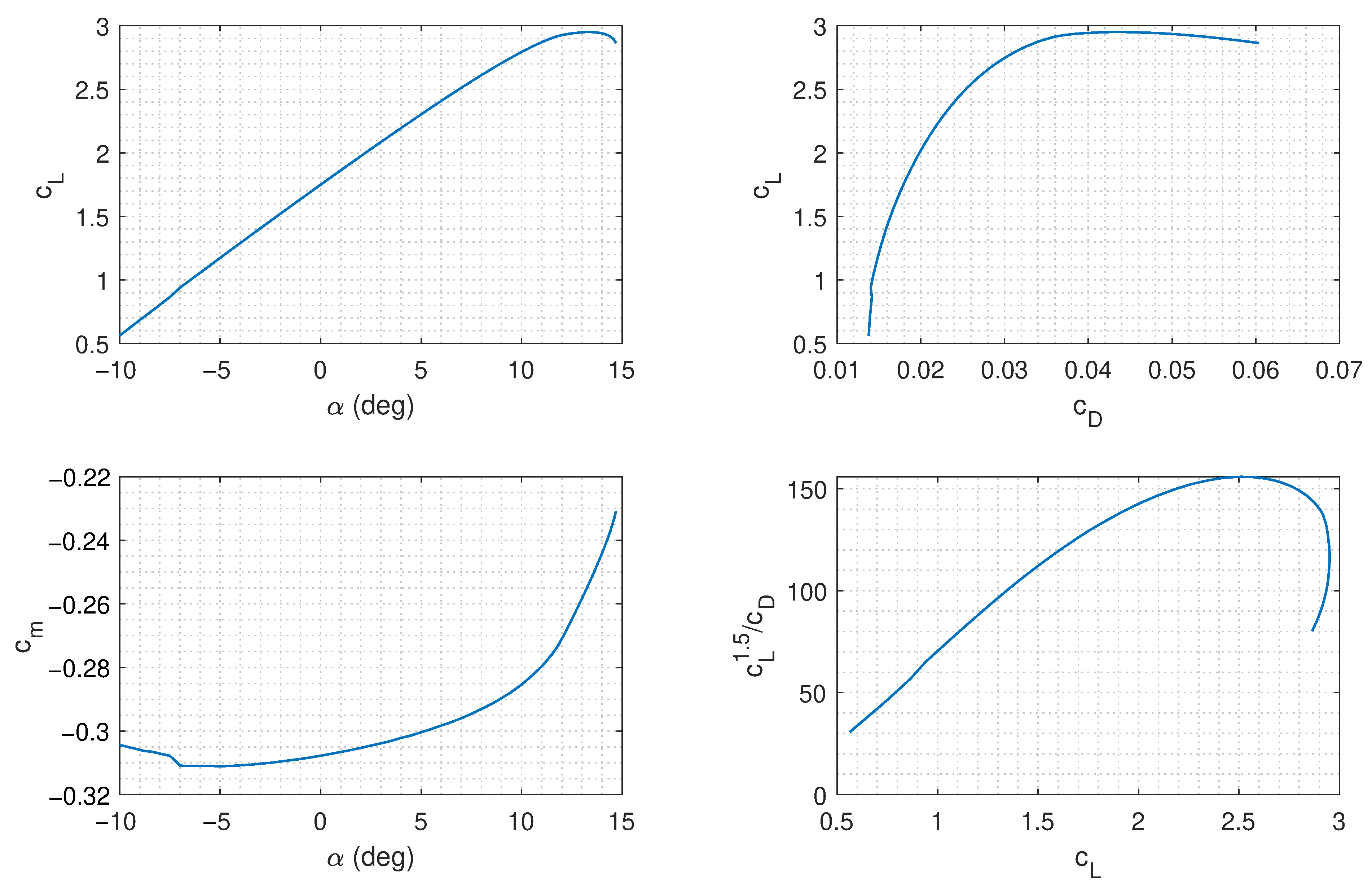
Section 3 presents the results, including the optimised airfoil in production- and return-phase configurations, as well as the verification using CFD.
Section 4 concludes this study.
2. Methodology
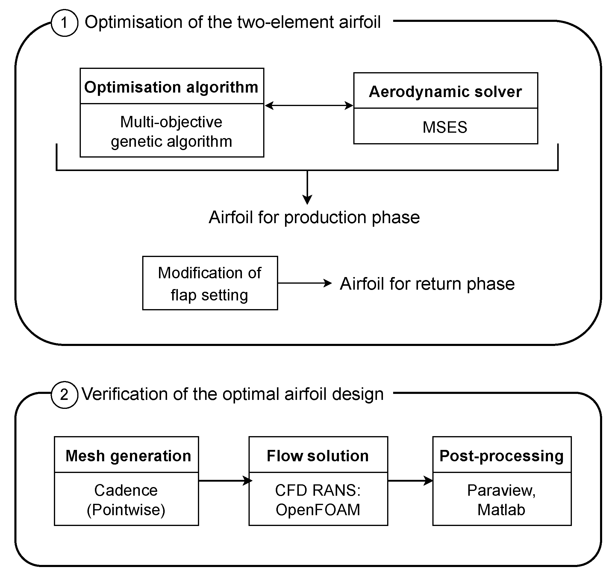
The optimisation procedure illustrated in
Figure 4 was presented in [
26] and is commonly used for the optimisation of multi-element airfoils.
In the first step, which is described in more detail in
Section 2.1, a multi-objective genetic algorithm was employed to optimise the multi-element airfoil shape and the flap setting (the relative position of the flap) for the production phases of the pumping cycles. A crucial requirement for a successful optimisation is a suitable description of the full airfoil geometry with a limited set of parameters that provide sufficient flexibility and shape control in the regions of interest. For the present study, the integration of the flap was of particular importance because the flap setting is used to transition from the power to the return phases. Another crucial element for optimisation is the definition of the optimisation goals used to construct the objective functions for the optimisation algorithm. These functions are designed to maximise the generated power in the production phases. The genetic algorithm was implemented in Matlab from where the aerodynamic solver executable was called. The aerodynamic performance of the resulting airfoil was then analysed for the return phase and the flap setting was modified to minimise the lift of the airfoil. Accordingly, the airfoil will have different flap settings for the different phases, leading to an airfoil designed with two different configurations.
In the second step, which is described in more detail in
Section 2.2, the aerodynamic performance of the resulting airfoil was verified using higher-fidelity but computationally more expensive CFD simulations. The verification of the airfoil polars was performed for both configurations, the production and return phases.
2.1. Optimisation of the Two-Element Airfoil
This section presents the details of the optimisation procedure, including the optimisation objectives, parametrisation scheme, optimisation algorithm, and aerodynamic solver.
2.1.1. Optimisation Objectives
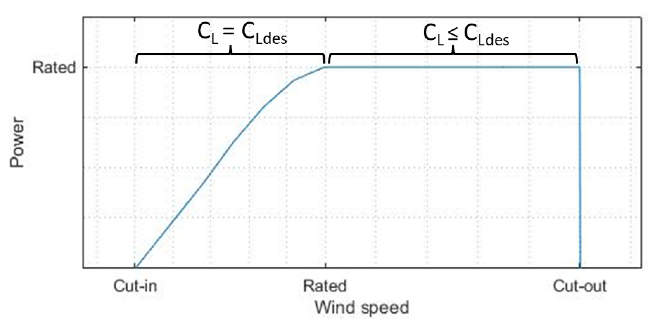
The optimisation objectives for the production phases of the pumping cycles were closely linked to the implemented control strategy of the AWE system [
29], which is illustrated in
Figure 5 as a schematic power curve of the system, together with the two ranges of the set values for the lift coefficient
.
Below the rated wind speed, a system is operated at the design lift coefficient of the airfoil. Maximising also maximises the pulling force of the kite at a specific wind speed. A physical upper limit is the maximum lift coefficient at which the airfoil begins to stall. To ensure the safe operation of the kite, the present study limited to 80% of the maximum lift coefficient and avoided getting anywhere close to this condition. Consequently, the primary optimisation objective was the maximisation of to maintain a high during operation. Above the rated wind speed, the tether force and generated power can no longer be effectively limited by reeling out faster. In this wind speed regime, the set value of the lift coefficient is decreased to limit the system loads. In the present study, the lift coefficient was lowered to 70% of and was considered representative of the operation above rated wind speed.
A secondary optimisation objective was to maximise the ratio
for both wind speed ranges. Therefore, the three objective functions for the production phase can be formulated as
where
is a set of design variables that fully defines the geometry of the airfoil, as described in
Section 2.1.2.
The return-phase airfoil configuration aims to reach a low such that the tether force is as low as possible and the consumed power is minimised. Such an objective is accounted for by modifying the flap setting during the return phase.
2.1.2. Parametrisation Scheme
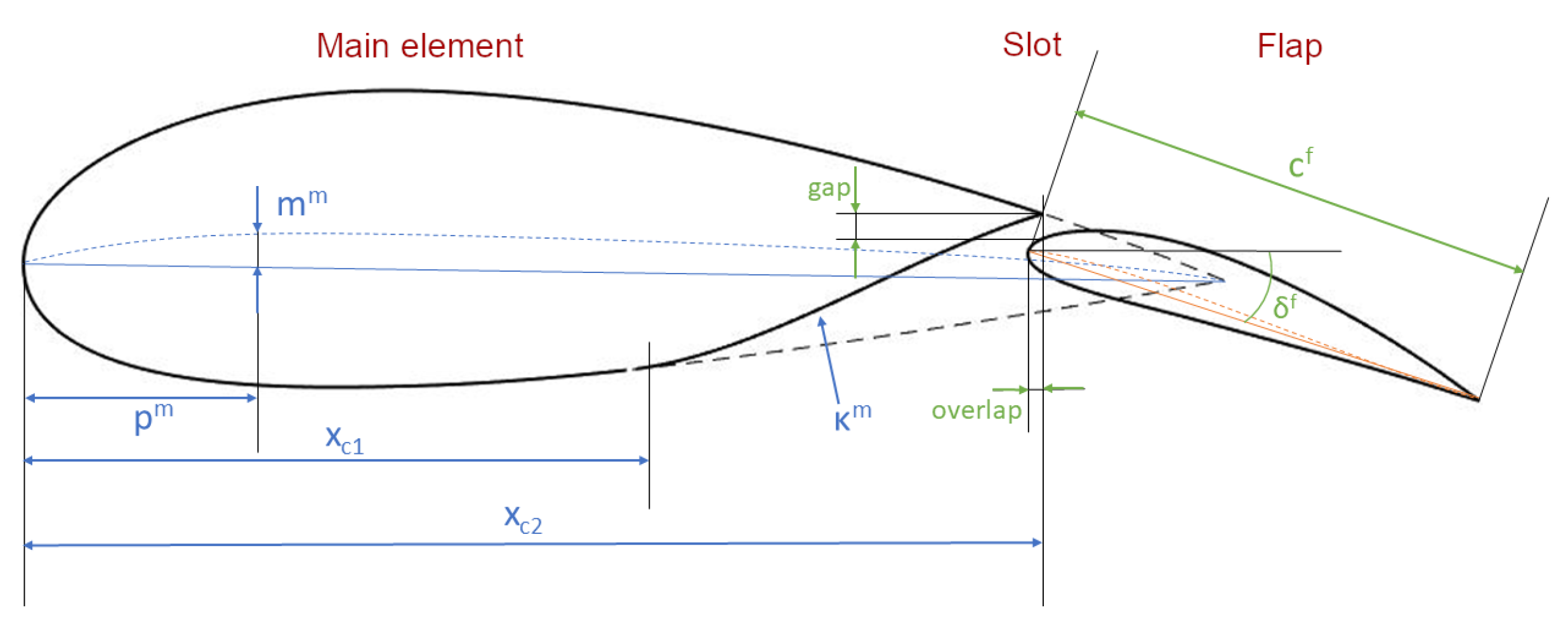
The purpose of the parametrisation scheme is to fully define the geometry of the multi-element airfoil using a set X of n scalar variables. Two types of design variables are distinguished: airfoil shape and flap-setting variables.
For efficient use in an optimisation procedure, the number of design variables should be as low as possible and the scheme should be flexible enough to allow for good shape control. A high degree of flexibility is favourable for the main element since the aerodynamic performance is particularly sensitive to the slot shape, which is affected by the main element’s geometry at the trailing edge. Therefore, the simple NACA four-digit nomenclature was combined with a parameterised modification along the trailing edge. In the present work, this modification is referred to as a ‘cut’ and is defined by a 3rd-order polynomial, requiring three additional design variables: the starting location along the lower surface of the main element, the ending location along the upper surface of the main element, and the curvature of the cut. In this way, the number of shape-related design variables of the main element is kept relatively low and the design flexibility matches the specific problem of finding a suitable flap integration. The shape of the flap has a relevant effect on the overall performance but the NACA method is deemed flexible enough to define it. A key reason for selecting the NACA nomenclature for the flap and as a ‘backbone’ for the main element was that the thickness becomes straightforward to control. This is relevant because the airfoil thickness is determined mainly by the structural requirements and should thus be easily constrained in the optimisation procedure.
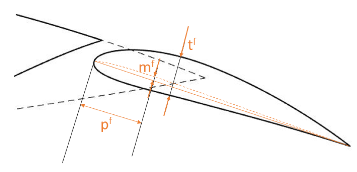
The relative position between the flap and the main element, denoted here as the flap setting, is defined by the flap overlap, gap, chord, and deflection. The gap is defined as the vertical distance between the main element’s trailing edge and the flap, whereas the overlap is the horizontal distance. The parametrisation requires a total of 12 design variables, as illustrated in
Figure 6 and
Figure 7 and listed in
Table 2. It should be noted that the main element thickness is not a design variable since it is given as a constraint. This constraint comes from the wing structural design since the thickness of the airfoil determines the thickness of the wing’s main spar.
2.1.3. Genetic Algorithm
A genetic algorithm is a stochastic metaheuristic optimisation technique inspired by the process of natural selection belonging to the larger class of evolutionary algorithms [
30,
31]. The working principle is based on a population of individuals, here airfoils, with their fitness quantified by one or more objective functions. The optimisation goal can be to maximise or minimise the values of the objective functions. As part of the selection process, the fitter individuals produce the next generation of airfoils through genetic operators, as illustrated in
Figure 8. Crossover is used to combine the genetic information of two parents to generate new offspring, whereas mutation is used to maintain the genetic diversity of the chromosomes in a population by randomly changing a property of an individual. Elitist selection automatically passes the best individuals to the next generation. This process of selection and variation is repeated until the algorithm meets the convergence criteria, which, in this case, is when the objective functions no longer improve.
Although a genetic algorithm is computationally expensive due to its population-based nature, it was selected over conventional gradient-based methods for its capability of dealing with multiple objectives in a very flexible manner (Pareto front) and its robustness in finding the global optima even in highly non-linear design spaces. For the present study, the Non-Dominated Sorting Genetic Algorithm II (NSGA-II) [
33,
34] was used. The algorithm is an extension of the general GA concept that aims to optimise multiple objective functions. Implementation in Matlab is provided through the use of the function
gamultiobj [
35], which allows for the easy control of the GA operators, including crossover and mutation. The population size was set to 20 individuals and the number of computed generations depended on the iterations needed to meet the convergence criteria.
2.1.4. Aerodynamic Solver
The optimisation procedure uses the two-dimensional aerodynamic solver MSES to evaluate the load distribution on a specific multi-element airfoil [
11,
12]. MSES is a viscous-inviscid interaction code that combines a finite-volume solver for the Euler equations in the inviscid part of the flow field with an integral formulation of the boundary layers and wake regions [
36]. The finite-volume mesh is generated automatically by intersecting the inviscid flow streamlines and splines emitting orthogonally from the airfoil surface, where the inviscid flow streamlines are precomputed using a panel method. This procedure results in a high-quality structured mesh since it attains satisfactory orthogonality. Moreover, the mesh parameters are user-defined so they can be tuned to reach a smooth grid with minimal skewness, and the cells’ aspect ratio is not too high. MSES was selected for the following reasons:
the automatically generated mesh (see
Figure 9) was of good quality and adapted well to variations of the geometry;
the computation time was short;
the executable ran without a graphical user interface and with input and output via text files, that is, it can be operated using scripts and can be easily combined with the genetic algorithm in Matlab;
the software is open source and can be used for academic purposes;
the solver produced fairly accurate results for the linear region of
and
, although there were larger errors for the
[
28,
37,
38].
A drawback of using MSES is that the solver does not always converge, which can be related to the occurrence of large flow-separation regions as a result of specific flow conditions, complex geometry, or a combination of both. Since convergence problems are undesirable in an automated optimisation process, the issue was mitigated by adjusting the bounds of the design variables and finding mesh parameters that could produce a high-quality mesh for a wide range of geometries. Moreover, a human-in-the-loop approach was employed by manually monitoring and controlling the optimisation algorithm to ensure that all aerodynamic analyses converged.
2.1.5. Flow Conditions
The optimisation was run under specific flow conditions representative of the conditions experienced by the kite during operation. The relevant flow conditions to be determined were the Reynolds number and the boundary layer type (laminar or turbulent). The representative flow speed for the kite system operation was
= 45 m/s. Although the kite can operate at a wide range of speeds, a reference value needed to be chosen for this design phase. The density
and dynamic viscosity
were taken at a reference temperature of 15°, leading to the values
=
kg/m
and
=
kg/(ms). The reference length, which was provided by the company, was representative of the whole wing. Since the wing has varying chords in the spanwise direction, an estimation of the mean aerodynamic chord (MAC) was utilised, which was assumed to be close to a length of
m. By substituting in the Reynolds number equation, we obtain
which was utilised for the whole optimisation procedure for both the MSES and RANS simulations. From the company’s perspective, the leading edge of the kite wing would become dirty after a certain period of time and would remain so during prolonged operation. Deposits on the wing’s LE can trigger turbulent flow in the boundary layer. Therefore, a fully turbulent boundary layer was used for the airfoil optimisation, even though it might partially remain laminar during periods of operation when the LE is clean. This approach is considered conservative since a turbulent boundary layer is known to increase the viscous drag on the airfoil’s surface [
39].
2.2. Verification of the Optimal Airfoil Design
Once the optimal design of the multi-element airfoil was identified, its aerodynamic performance was verified through RANS simulations. The workflow of the higher-fidelity toolchain is illustrated in the bottom part of
Figure 4 as progressing from mesh generation to flow solution and eventually post-processing.
2.2.1. Setup of RANS Simulations
The finite-volume mesh was generated using the commercial meshing software Cadence, formerly known as Pointwise. The software can be used with its own scripting language Glyph to efficiently construct high-quality meshes of parametrised geometries.
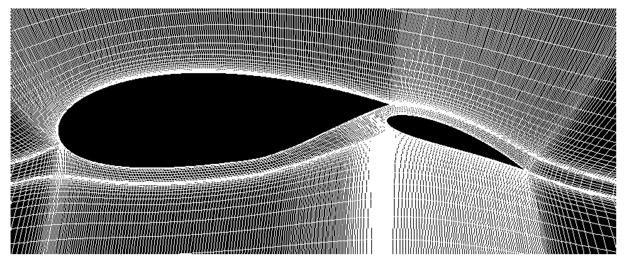
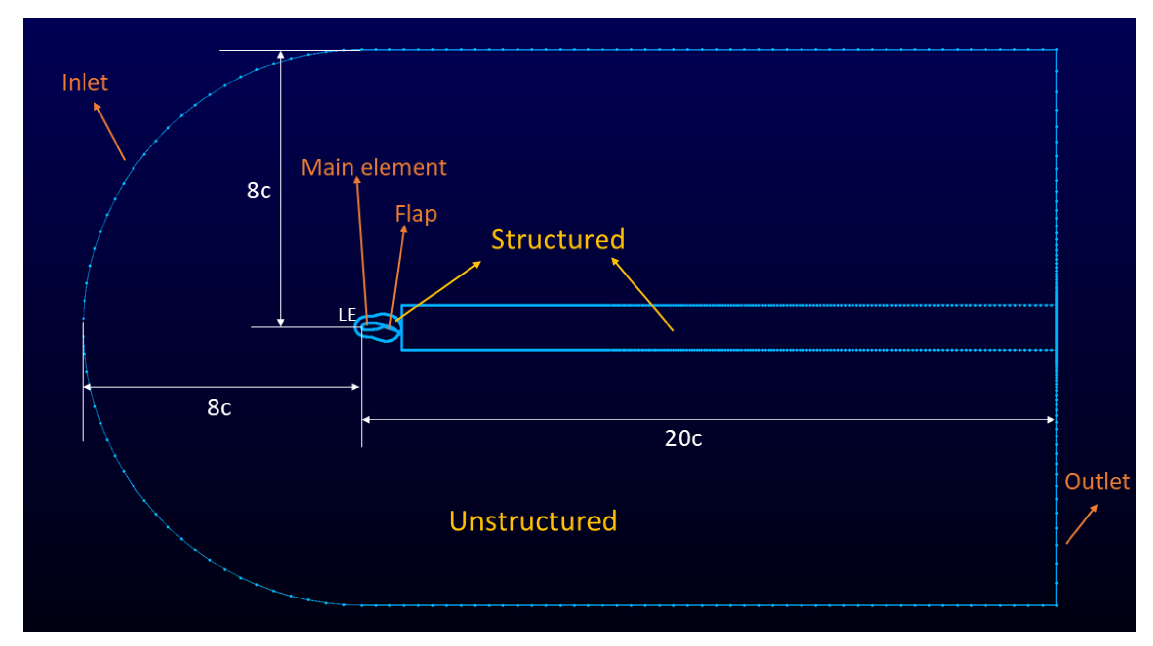
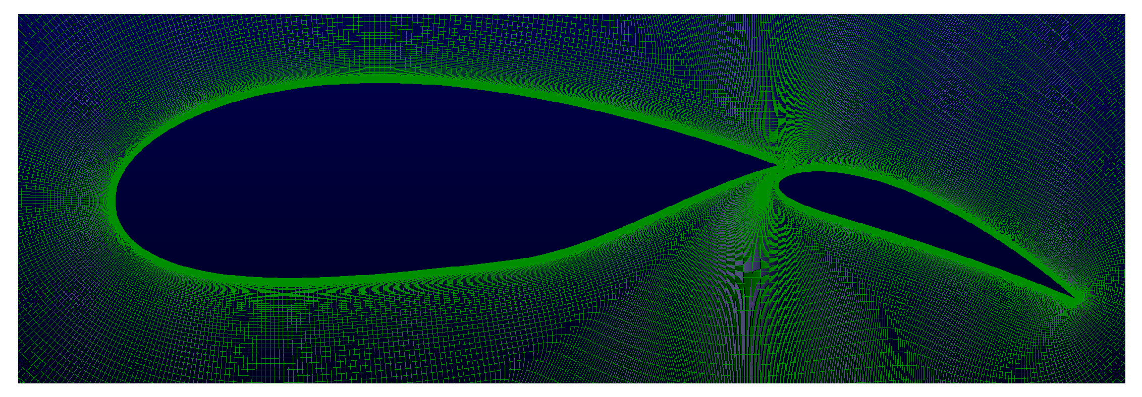
Figure 10 shows the topology of the generated hybrid mesh structured around the airfoil and in the wake and unstructured otherwise. The body-fitted O-grid mesh was generated through hyperbolic extrusion such that the first cell layer is orthogonal around the surface of both elements, as shown in
Figure 11.
This approach allowed us to easily adjust the non-dimensional height
of the first cell layer, which was determined through a mesh sensitivity analysis, by progressively decreasing the value of
to investigate the effect on the aerodynamic coefficients
and
. The baseline case employed for such a procedure is a NACA 2424 airfoil at
. With the reduction of
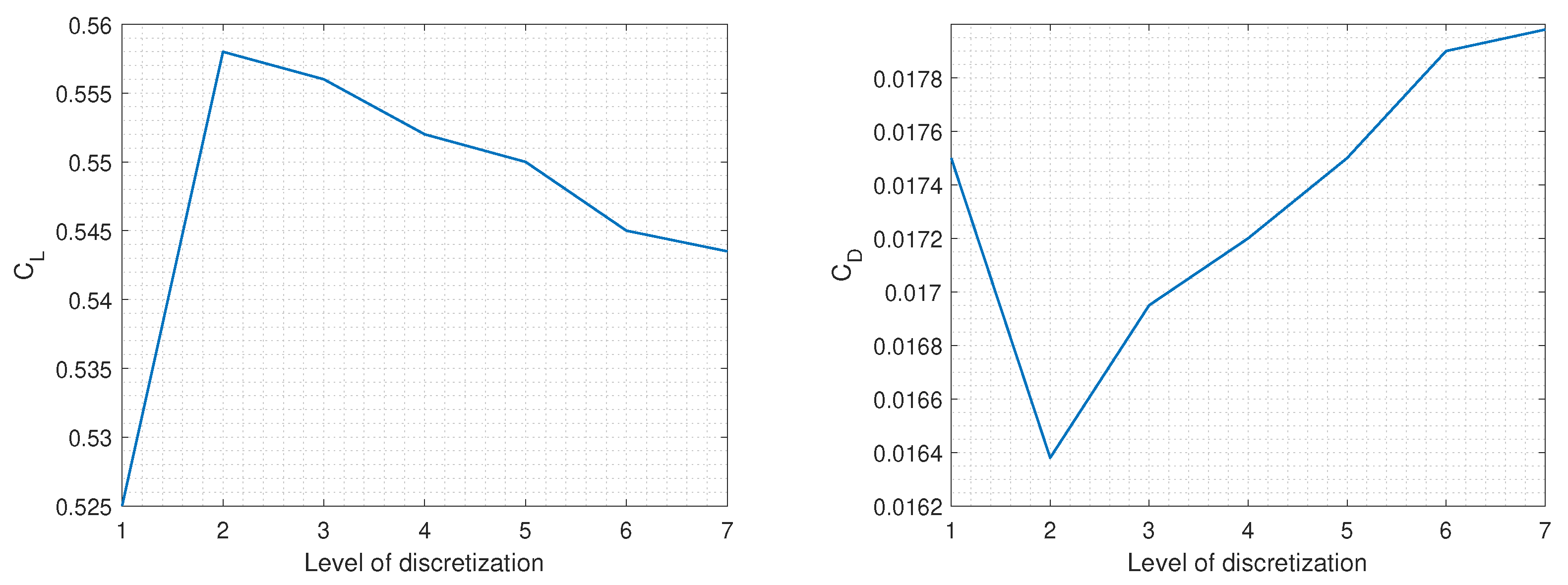
, the length of the cells along the surface was decreased to maintain the cell aspect ratio within reasonable bounds. The mesh sensitivity of the computed aerodynamic coefficients is shown in
Figure 12 and
Table 3.
Figure 12 shows that the mesh sensitivity of the aerodynamic coefficients weakens for values of
below
. Notice that the relative variation of the lift coefficient above the second level of refinement, i.e., below
, is less than 3%. On the other hand, the drag coefficient varies significantly in that same range, with a variation close to 9%, indicating that it is preferable to employ a small
of around 0.2 to reduce the effect of the mesh resolution.
Following the generation of the mesh, the flow field was computed using the open source software OpenFOAM with the steady-state solver SimpleFoam for the incompressible turbulent flow. The
k-
SST turbulence model [
40] was used to close the RANS equations because of its superior performance for both external flows and boundary layers. The model employs two additional transport equations, one for the turbulence kinetic energy
k and one for the specific turbulence dissipation rate
. It cannot model the transition from laminar to turbulent flow and, consequently, assumes that the boundary layer is fully turbulent, which adapts well to our problem, as stated in
Section 2.1.5. This specific combination of physical models was recommended by [
19,
26] for the aerodynamic analysis of conventional airfoils and by [
41] for the analysis of a leading-edge inflatable kite airfoil.
The numerical scheme used for the time derivative terms was a second-order implicit (backwards), whereas the gradient and divergence terms were computed through the linear interpolation of values from cell centres to face centres (Gauss linear).
The CFD results were post-processed using the open source software Paraview, mainly to illustrate and investigate the flowfield around the airfoil. Convergence plots or the surface pressure distribution along the airfoil were computed using Matlab scripts.
2.2.2. RANS Simulation Validation
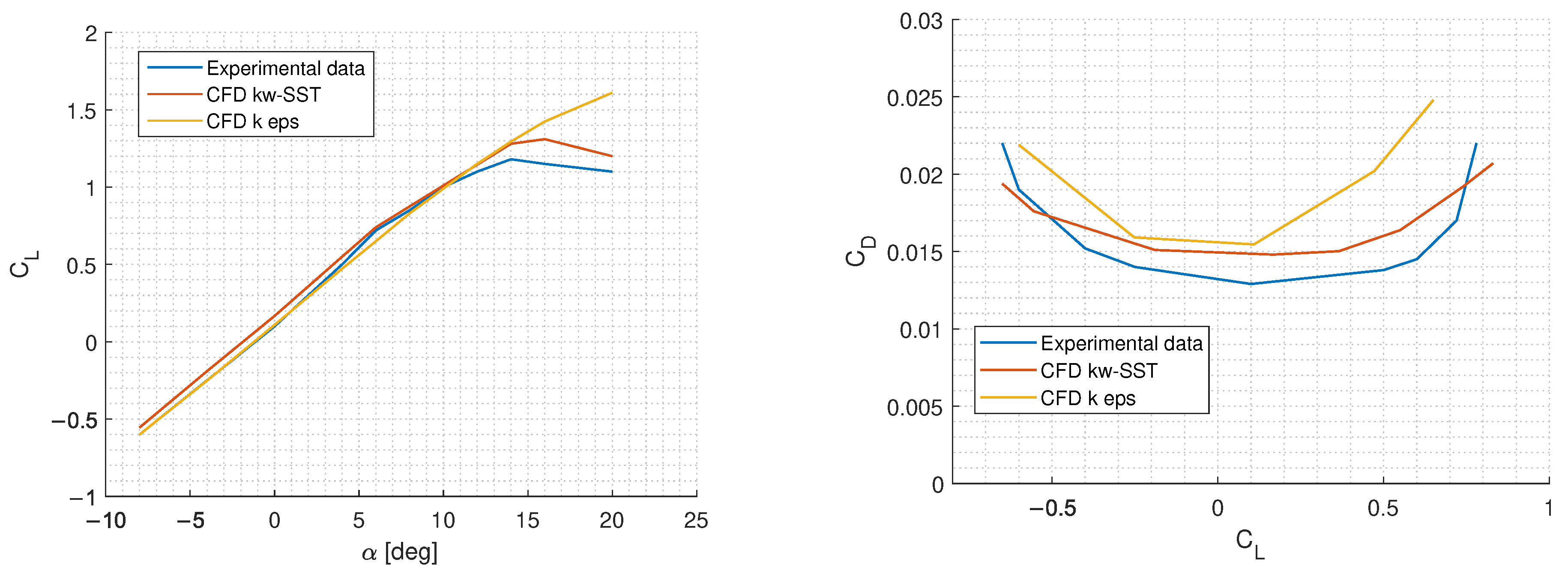
Before verifying the computed MSES polars with OpenFOAM, the CFD solver was validated with a simple test case to quantify its accuracy with respect to the experimental data. The simulation case for this validation was an NACA 2424 at
, where the experimental polars were obtained from [
42]. The comparison of the computed and measured data is shown in
Figure 13, including the simulation results obtained using the
SST and
turbulence models.
The comparison shows that the SST turbulence model performs significantly better, accurately predicting the lift coefficient in the linear region and capturing also fairly well the stall region, while only slightly overpredicting the maximum lift. The model clearly overestimates the drag but still stays rather close to the experimental data, roughly within 13% of relative error. The turbulence model is also accurate in terms of lift in the linear region but is not capable of capturing the flow separation in the stall region, and drag is significantly overpredicted for the entire range.
4. Conclusions
This paper describes an optimisation approach for a two-element airfoil of a fixed-wing airborne wind energy system that is operated by pumping cycles. The production and return phases of the cycles have distinctly different design requirements. To account for this, the airfoil geometry is first optimised for the production phases, followed by an adjustment of the flap setting to ensure its efficient performance in the return phases. The aerodynamic performance of the resulting airfoil was verified by comparing the computed lift and drag polars with higher-fidelity RANS simulations.
The developed parametrisation scheme provides flexible shape control with a limited set of design variables. The scheme combines the NACA four-digit nomenclature for both elements with a modification of the main element’s trailing edge geometry to enhance the integration of the flap and control the shape of the slot. Moreover, the scheme facilitates the constraining of the thickness of the elements, which is required for structural reasons.
The multi-objective genetic algorithm NSGA-II proved to be robust and efficient in finding the global optima in the highly non-linear design space and providing a Pareto front to make tradeoffs for choosing an optimal airfoil design. The gradient-free optimisation method was able to cope with missing sensitivity information in regions of the design space caused by occasional convergence problems of the aerodynamic solver MSES. Although it was possible to avoid such convergence problems in many cases by carefully adjusting the mesh parameters, complete elimination was not possible. The unfavourable effect of unconverged MSES runs was mitigated by employing a human-in-the-loop technique, with the designer monitoring and analysing the problematic cases so that the optimisation algorithm could continue. However, MSES was selected as an aerodynamic solver for the optimisation because of its low computational cost, fairly accurate results, and ease of integration with an optimisation algorithm. Furthermore, MSES can automatically generate a hyperbolic mesh of high quality, which is particularly useful for complex multi-element airfoil geometries.
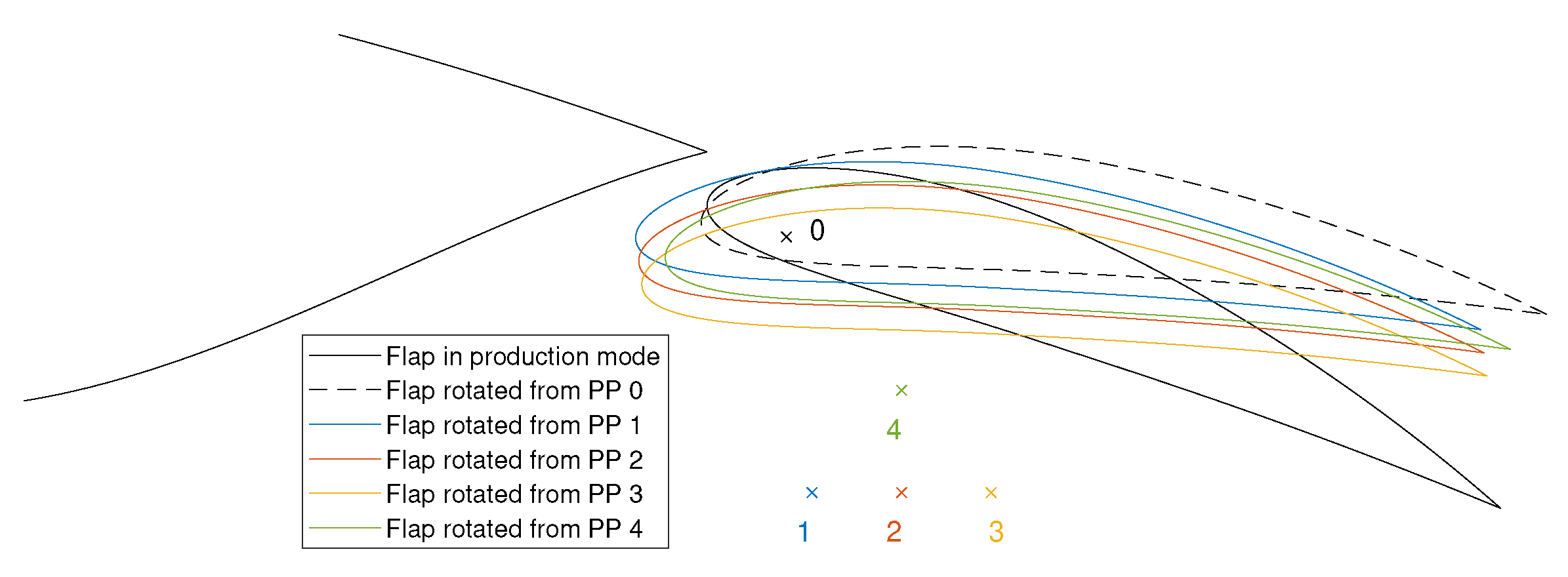
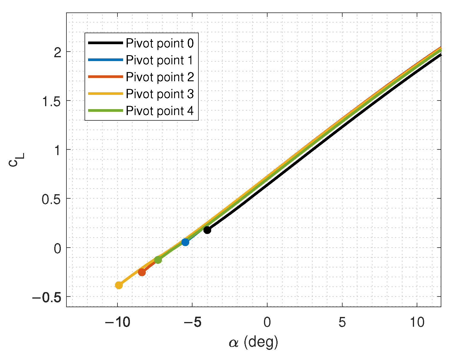
To maximise the power output of the production phase, three objective functions were prioritised. The highest-priority objective was the maximisation of the operational , whereas the maximisations of the ratio for wind speeds below and above the rated wind speed were of secondary importance. The lift and drag polars indicated a satisfactory performance of the optimised airfoil in the production phase. For the return phase, the lift coefficient of the airfoil was minimised by rotating the flap upwards around a specific pivot point so that the flap-up configuration had a certain overlap with the main element. This specific geometric feature induced a high-velocity flow that re-energised the boundary layer on the main element and mitigated flow separation. Practically, the overlap can be created by placing the pivot point outside the flap so that the flap is rotated and translated at the same time. The optimisation resulted in a two-element airfoil with satisfactory performance for both the reel-out and reel-in phases achieved using a movable flap. Such a mechanism is crucial for the development of AWE systems so that the entire operational cycle can be efficiently performed.
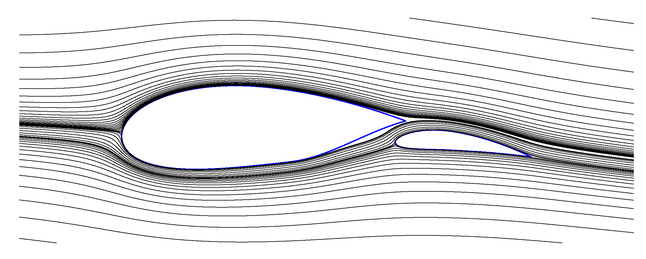
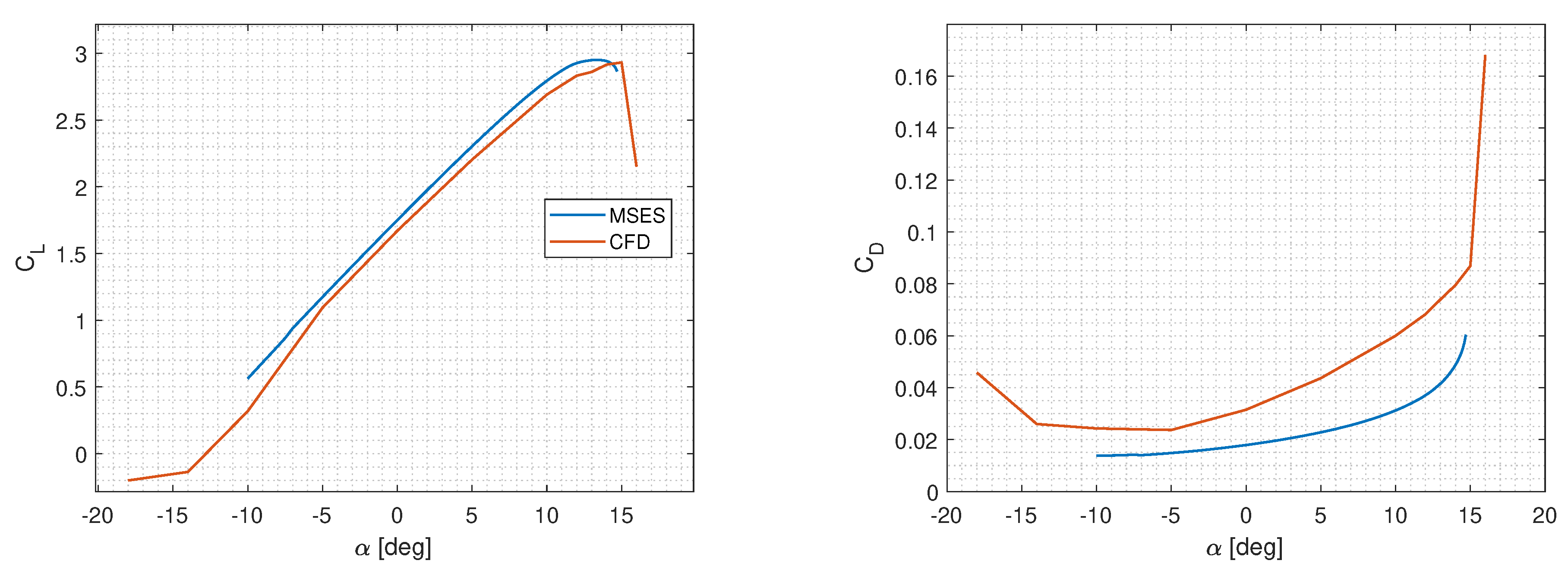
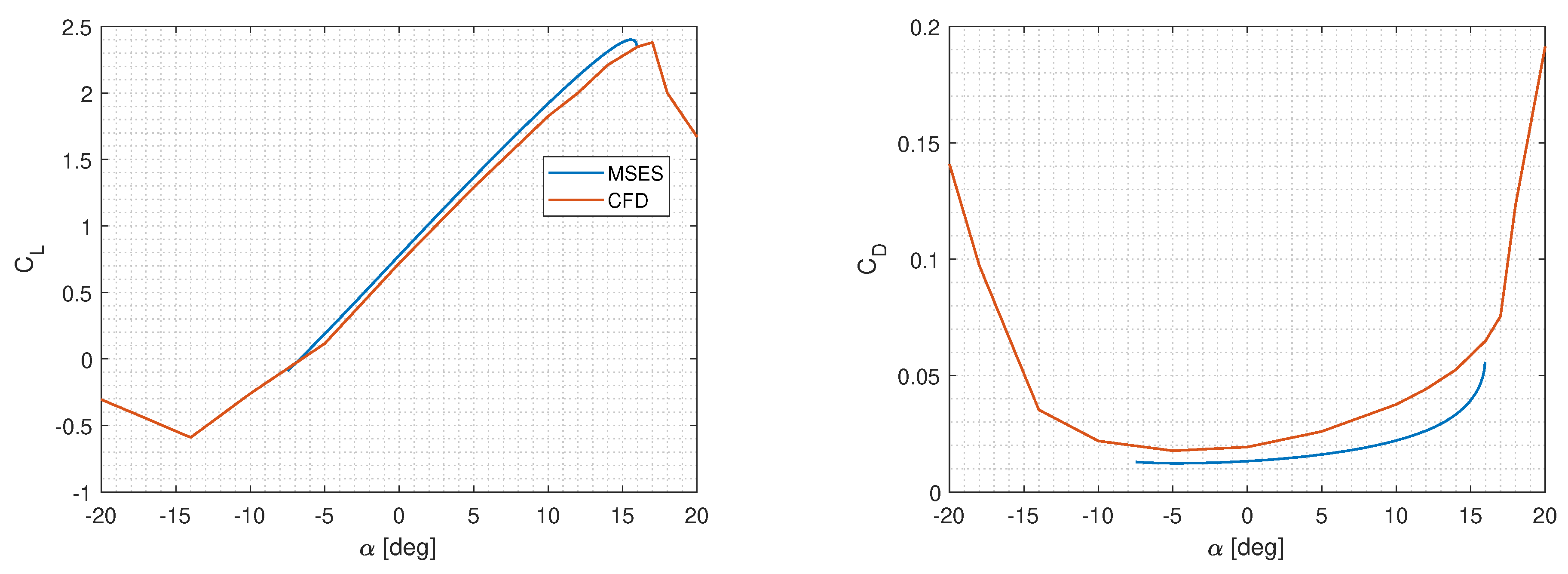
The CFD setup was first validated using the experimental data of a single-element airfoil, NACA 2424, which showed fairly good agreement. The SST turbulence model was selected because of its superior performance in dealing with both external and boundary layer flows. The verification results showed good agreement for the lift coefficient both in the linear region and for . On the other hand, the drag coefficient was significantly underpredicted by MSES. The flow separation phenomena in the return phase were also investigated through CFD simulations. The performance improvement achieved by varying the location of the flap pivot point based on MSES analyses is supported by the flow field visualisations obtained from CFD.
Regarding recommendations for future work, several areas could be extended. This work studied two-element airfoils to meet the high-lift requirements of an AWE system. However, it may be worth investigating three-element airfoils to evaluate the trade-off between the added complexity and aerodynamic improvement. Furthermore, adding validation with a multi-element airfoil would help to determine whether the agreement with the experimental data varies with the addition of an element. Finally, conducting an experimental simulation on the optimised airfoil would be highly beneficial in assessing the accuracy of the solvers used in this study.


