Bacterial Foraging Algorithm for a Neural Network Learning Improvement in an Automatic Generation Controller

Abstract

The frequency diversion in hybrid power systems is a major challenge due to the unpredictable power generation of renewable energies. An automatic generation controller (AGC) system is utilised in a hybrid power system to correct the frequency when the power generation of renewable energies and consumers’ load demand are changing rapidly. While a neural network (NN) model based on a back-propagation (BP) training algorithm is commonly used to design AGCs, it requires a complicated training methodology and a longer processing time. In this paper, a bacterial foraging algorithm (BF) was employed to enhance the learning of the NN model for AGCs based on adequately identifying the initial weights of the model. Hence, the training error of the NN model was addressed quickly when it was compared with the traditional NN model, resulting in an accurate signal prediction. To assess the proposed AGC, a power system with a photovoltaic (PV) generation test model was designed using MATLAB/Simulink. The outcomes of this research demonstrate that the AGC of the BF-NN-based model was effective in correcting the frequency of the hybrid power system and minimising its overshoot under various conditions. The BP-NN was compared to a PID, showing that the former achieved the lowest standard transit time of 5.20 s under the mismatching power conditions of load disturbance and PV power generation fluctuation.

1. Introduction

Due to the air pollution and energy crisis, renewable energies have become substantial sources in the power system to replace conventional energy sources. Typically, the power generation of a hybrid power system consists of classical energy sources and renewable energy sources applied in a multi-area power system that is connected through power-lines [1,2,3,4]. Owing to the unpredictable power generation of renewable energies and the variation in load demand, an automatic generation controller (AGC) is designed to restore the frequency level of a hybrid power system when consumers’ load demand and renewable energy sources swiftly fluctuate by regulating the speed governor of the classical generator [5,6,7,8,9]. Additionally, renewable energy sources have less inertia to integrate with the power system, which makes the power imbalance worse by causing tie-line power oscillations in multi-area system [10,11,12].

Recently, several researchers have proposed various AGCs based on classical and advanced techniques for hybrid power systems. Among these, the authors of [13] utilised a PID with an H∞ controller to design an AGC for a hybrid micro-grid power system. The H∞ controller was proposed to regulate the nonlinearity of the hybrid power system when the load demand and the wind power generation change rapidly. The outcomes of this work show that the proposed method reduced the frequency deviation in the range of ±10% to ±30% with respect to the standard value. Furthermore, the authors of [14] tested two types of AGC for a hybrid mica-grid power system based on H∞ and µ-synthesis techniques. The hybrid power system was connected to a diesel generator, a wind turbine, and a fuel cell. The results showed that the µ-synthesis AGC method was better to offset the frequency diversion of the hybrid power system in comparison to the H∞ method. However, AGCs based on classical techniques are not able to reset the frequency diversion of hybrid power systems sufficiently when the renewable energy source is changed suddenly due to a poor dynamic model [15,16,17,18]. Hence, advanced machine learning algorithms have been proposed to solve this issue since they do not demand high-level mathematics when applied to complex applications such as AGCs [19,20,21].

Fuzzy logic control (FLC) has been widely used to design optimal AGCs because of its nonlinear model [22]. Consequently, the authors of [23] designed a secondary frequency control using an adaptive neuro-fuzzy inference system (ANFIS) for a hybrid micro-grid power system. Simulation results demonstrated that the ANFIS control reset the frequency of the proposed system using several load variations. Similarly, the authors of [24] designed an AGC based on an adaptive fuzzy logic PID controller, which was optimised using a sine/cosine algorithm to address the high oscillation in the frequency caused by unpredictable renewable energy generation. The results show that this proposed controller has a superior improvement compared to the PID controller. Furthermore, the authors of [25] used FLC with a proportional–integral–derivative technique to design an efficient AGC for a hybrid power system. A cuckoo search algorithm was used to tune the parameters of the FLC-PID controller. Simulation results based on Lab-View have showed that the proposed AGC was fit to offset the frequency diversion when the load disturbance changed rapidly when connected to renewable energy sources. However, this technique requires good experimental knowledge to tune the FLC model. In addition, it requires a long processing time to correct the signal when used with unpredictable resources such as renewable energies. To overcome this unpredictable challenge, an intelligent method based on training data instead of experimental knowledge has been employed to design an optimised AGC.

The authors of [26] designed an AGC for a three-area hybrid power system using the grey wolf optimiser PID technique. The proposed system is quite robust in terms of the transit time, overshoot, and oscillations of the frequency system with or without being connected to renewable energy sources. Similarly, the authors of [27] used particle swarm optimisation (PSO) to tune linear matrix inequality to design an AGC for a multi-hybrid power system. The outcome of this work shows that wind power generation has the highest fluctuation when compared to other renewable power generation. Similarity, the authors of [28] also used a PSO algorithm to design an AGC for a power system using wind turbines. Simulation results of the proposed method show that the frequency stability of the system is significantly improved when used with and without wind power generation under various conditions. Furthermore, the authors of [29] utilised a social-spider optimiser (SSO)-PID to design an AGC for a two-area hybrid power system. The results demonstrated that the SSO-PID controller reset the frequency diversion of the hybrid power system quickly compared to the GA-PID controller. Next, the authors of [4] used a neural network (NN) technique to predict the frequencies of an AGC for a two-area power system. The NN was optimised using a PSO algorithm to select the number of hidden layers and the connection weights. The combination of renewable energies with a classical power system network suffers from frequency diversion due to the changes in load demand and renewable power generation. Hence, the design of an optimal AGC for a hybrid power system is required to produce fast and accurate responses to meet the load demand and the unpredictable power generation of renewable energies.

In this paper, a bacterial foraging (BF) algorithm is employed to design an AGC based on an NN for a hybrid power system that is connected with a photovoltaic (PV) energy resource. The novelty of this work is the use of a BF algorithm to optimise the elementary weights of the NN model, which minimises the NN training error. Consequently, the frequency diversion of the hybrid power system is addressed quickly, and its overshoot is minimised adequately since the BF algorithm has a fast response time. This results in a low transit time when tested in the mismatching power conditions of load disturbance and PV power generation. The rest of the work is structured as follows: Section 2 presents the modelling of the hybrid power system based on an AGC. Section 3 explains the main concepts of the NN model and the BF algorithm. Then, Section 4 describes the proposed method. Section 5 discusses the results of the proposed AGC under four case conditions. Finally, Section 6 concludes with the main findings of this research.

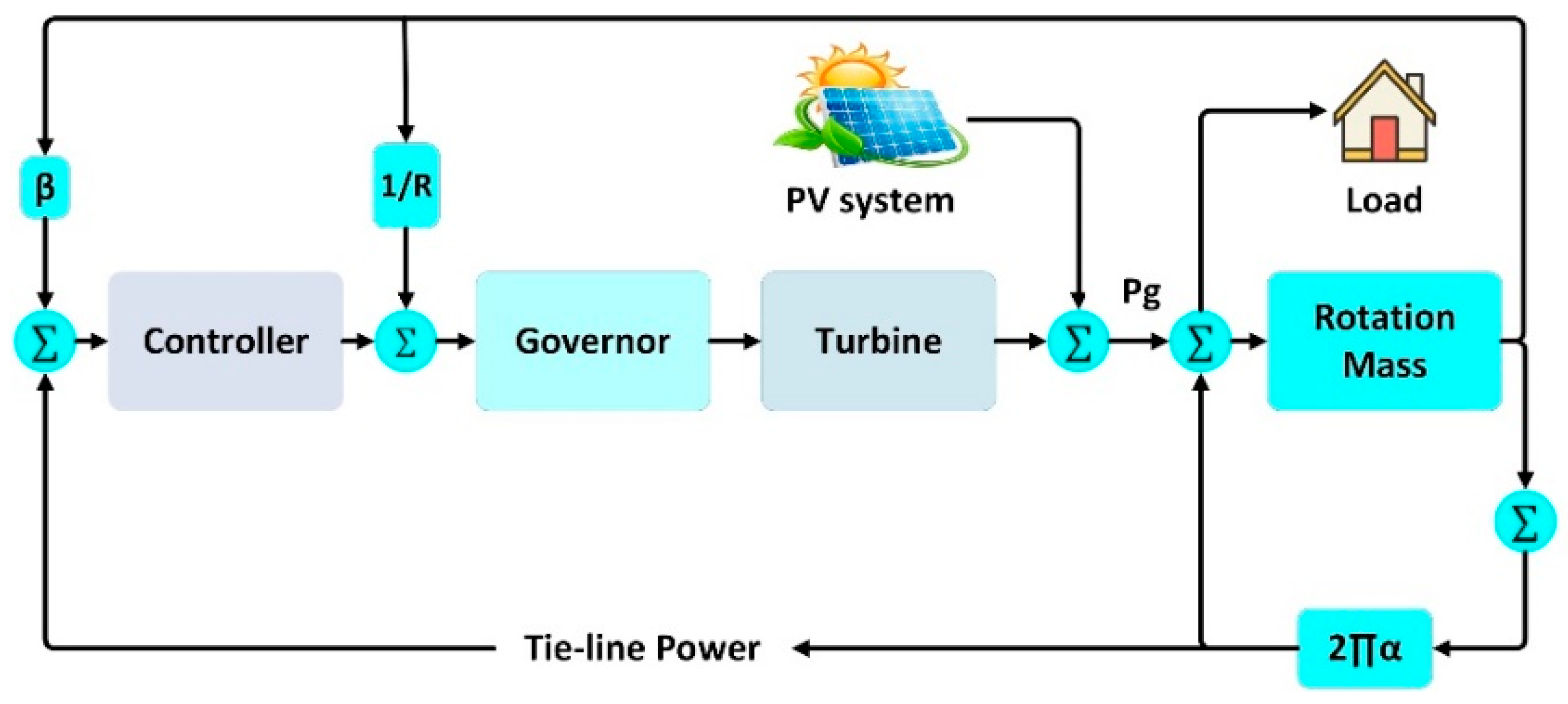
2. Modelling of Hybrid Power System

In this section, a traditional power system with a PV source is modelled, which consists of a thermal turbine, a generator, and a grid-connected PV system.

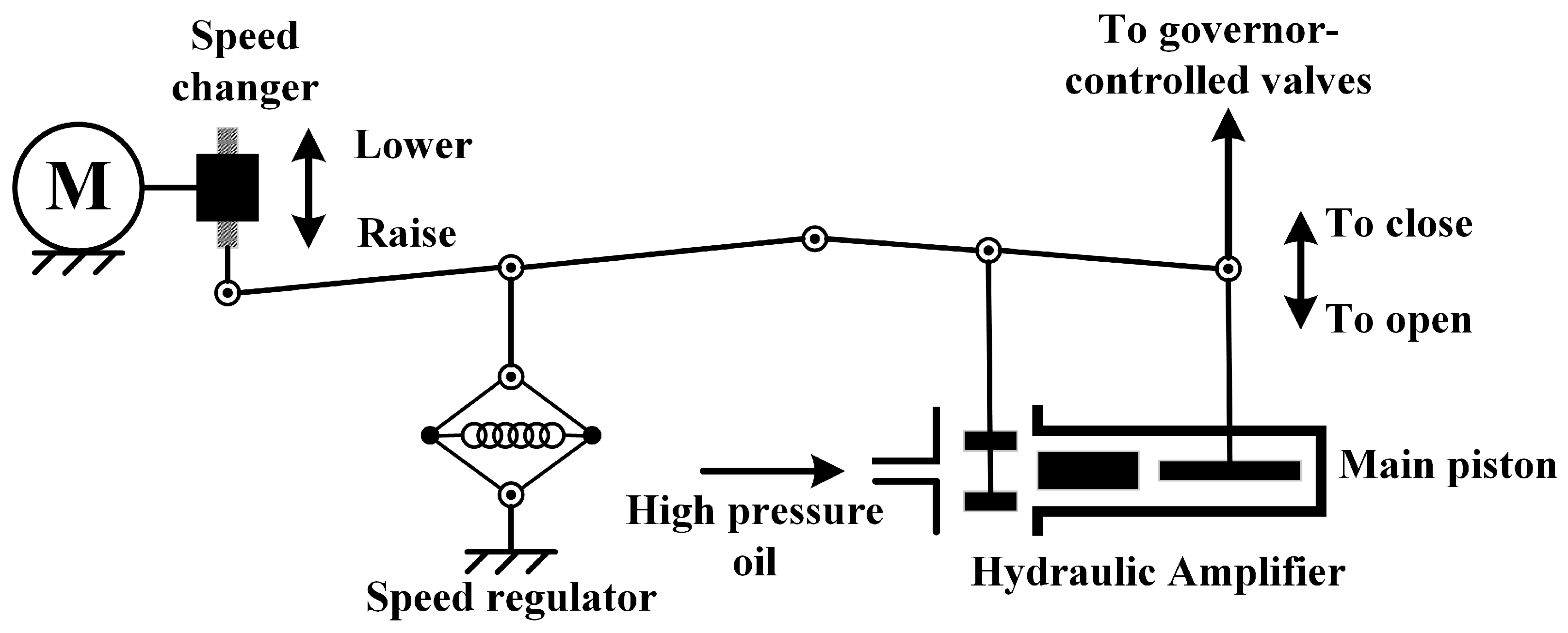
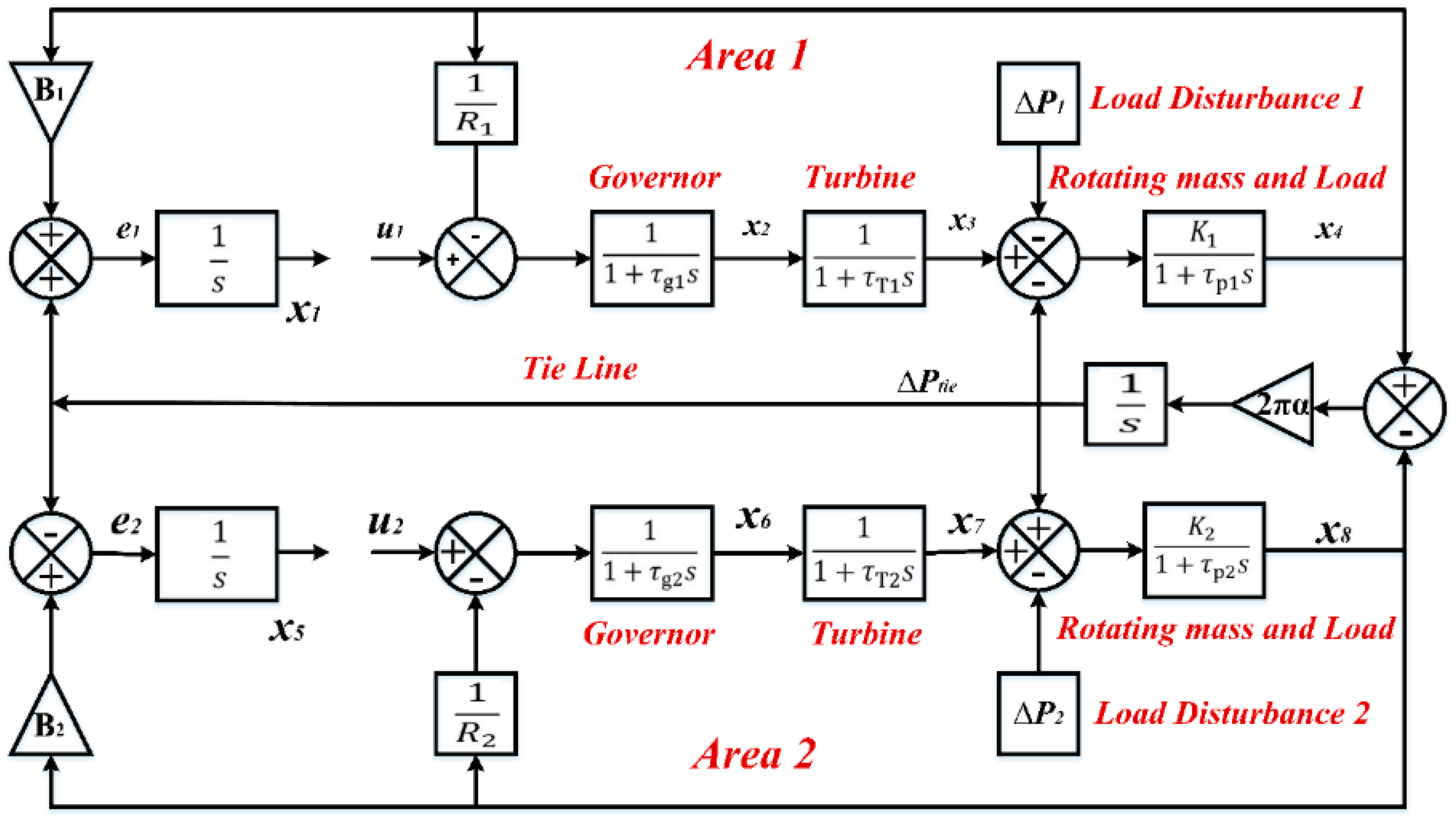
2.1. Modelling of Power System

Basically, the thermal turbine produces the mechanical power to generation the electrical power for the customer based on the steam fuel. A governor is a main component of a steam turbine, as presented in Figure 1.

To adjust the power generation with respect to the costumer load, the volume of the turbine steam is adjusted using the governor. Consequently, the speed of the generator is regulated, and the frequency response of the power system resets to offset the standard value of the power system, as proposed in Equation (1):

$$\Delta \mathit{f}=\left(\frac{\mathbf{1}}{\mathbf{2}\mathit{H}}\right)\Delta {\mathit{P}}_{\mathit{m}}-\left(\frac{\mathbf{1}}{\mathbf{2}\mathit{H}}\right)\Delta {\mathit{P}}_{\mathit{L}}-\left(\frac{\mathit{D}}{\mathbf{2}\mathit{H}}\right)\Delta \mathit{f}$$

(1)

The mathematical representation of the generator’s speed depends on Equation (2):

$$\Omega \left(\mathit{s}\right)=\frac{\mathbf{1}}{\mathbf{2}\mathit{H}\mathit{s}}\left(\Delta {\mathit{P}}_{\mathit{m}}-\Delta {\mathit{P}}_{\mathit{e}}\right)$$

(2)

The costumer load is modelled based on Equation (3):

$$\Delta {\mathit{P}}_{\mathit{e}}=\Delta {\mathit{P}}_{\mathit{L}}+\Delta \mathit{\omega }$$

(3)

while the mechanical power of turbine is modelled based on Equation (4):

$$\frac{\Delta {\mathit{P}}_{\mathit{m}}\left(\mathit{s}\right)}{\Delta {\mathit{P}}_{\mathit{v}}\left(\mathit{s}\right)}=\frac{\mathbf{1}}{\mathbf{1}+{\mathit{\tau }}_{\mathit{g}}\left(\mathit{s}\right)}$$

(4)

Lastly, the speed error of the governor is modelled based on Equation (5):

$$\Delta {\mathit{P}}_{\mathit{g}}=\Delta {\mathit{P}}_{\mathit{r}\mathit{e}\mathit{f}\mathit{.}}-\frac{\Delta \Omega \left(\mathit{s}\right)}{\mathit{R}}$$

(5)

To reset the frequency level of the power system, the AGC is designed to adjust the turbine speed based on the load. The two-area power system is modelled using state-space equations, as shown in Figure 2.

The main nomenclatures of the two-area power system are illustrated in

Table 1. Nomenclatures of the two-area power system.

Parameters	Definition
Δf	Historical change in frequency
ΔPtie	Historical change in tie-line power
R	Regulations of governor
G	Controller gain
Pg	Output power of generator
u1 and u2	Control inputs in areas 1 and 2
ΔPg1 and ΔPg2	Historical change in output power of governor
ΔPt1 and ΔPt2	Historical change in output power of turbine
ΔP1 = D1	Load Disturbances in area 1
ΔP2 = D2	Load Disturbances in area 2
K1 and K2	Constants of areas 1 and 2
𝝉P1 and 𝝉P2	Time constants of areas 1 and 2
B1 and B2	Tie-line frequency bias in areas 1 and 2
𝝉g1 and 𝝉g2	Time constants of governor for areas 1 and 2
𝝉T1 and 𝝉T2	Turbine time constants for areas 1 and 2

. First, the input signals of the AGC control are presented in Equations (6) and (7):

$${\dot{\mathit{u}}}_{\mathbf{1}}={\mathit{G}}_{\mathbf{1}}\left({\mathit{e}}_{\mathbf{1}}\right)={\mathit{G}}_{\mathbf{1}}\left({\mathit{B}}_{\mathbf{1}}{\mathit{x}}_{\mathbf{4}}+{\mathit{x}}_{\mathbf{9}}\right)$$

(6)

$${\dot{\mathit{u}}}_{\mathbf{2}}={\mathit{G}}_{\mathbf{2}}\left({\mathit{e}}_{\mathbf{2}}\right)={\mathit{G}}_{\mathbf{2}}\left({\mathit{B}}_{\mathbf{2}}{\mathit{x}}_{\mathbf{8}}-{\mathit{x}}_{\mathbf{9}}\right)$$

(7)

The state-space variables of the first area are presented in Equations (8)–(11):

$${\mathit{x}}_{\mathbf{1}}=\int {\mathit{e}}_{\mathbf{1}} \mathit{d}\mathit{t}$$

(8)

$${\mathit{x}}_{\mathbf{2}}=\Delta {\mathit{P}}_{\mathit{g}\mathbf{1}}$$

(9)

$${\mathit{x}}_{\mathbf{3}}=\Delta {\mathit{P}}_{\mathit{T}\mathbf{1}}$$

(10)

$${\mathit{x}}_{\mathbf{4}}=\Delta {\mathit{f}}_{\mathbf{1}}$$

(11)

while the state-space variables of the second area are presented in Equations (12)–(15):

$${\mathit{x}}_{\mathbf{5}}=\int {\mathit{e}}_{\mathbf{2}} \mathit{d}\mathit{t}$$

(12)

$${\mathit{x}}_{\mathbf{6}}=\Delta {\mathit{P}}_{\mathit{g}\mathbf{2}}$$

(13)

$${\mathit{x}}_{\mathbf{7}}=\Delta {\mathit{P}}_{\mathit{T}\mathbf{2}}$$

(14)

$${\mathit{x}}_{\mathbf{8}}=\Delta {\mathit{f}}_{\mathbf{2}}$$

(15)

Hence, the tie-line-connected power is represented by Equation (16):

$${\mathit{x}}_{\mathbf{9}}=\Delta {\mathit{P}}_{\mathit{t}\mathit{i}\mathit{e}}$$

(16)

Finally, a single vector matrix is presented to explain the state-space equations of the two-area power system, as shown in Equation (17):

$$\dot{\mathit{x}}=\mathit{A}\mathit{x}+\mathit{B}\mathit{u}+\mathit{C}\mathit{z}$$

(17)

where x is the state of the power system; u is the signal control of the AGC, and z is the load disturbance, while A and B are the parameter matrices of the system for the governor, turbine, and load with the AGC, as presented in Equations (18)–(20):

$$\mathit{A}=\left[\begin{array}{ccccccccc}\mathbf{0}& \mathbf{0}& \mathbf{0}& {\mathit{B}}_{\mathbf{1}}& \mathbf{0}& \mathbf{0}& \mathbf{0}& \mathbf{0}& \mathbf{1}\\ \mathbf{0}& \frac{-\mathbf{1}}{{\mathit{\tau }}_{\mathit{g}\mathbf{1}}}& \mathbf{0}& \frac{-\mathbf{1}}{{\mathit{\tau }}_{\mathit{g}\mathbf{1}}{\mathit{R}}_{\mathbf{1}}}& \mathbf{0}& \mathbf{0}& \mathbf{0}& \mathbf{0}& \mathbf{0}\\ \mathbf{0}& \frac{{\mathit{K}}_{\mathbf{1}}}{{\mathit{\tau }}_{\mathit{p}\mathbf{1}}}& \frac{-{\mathit{K}}_{\mathbf{1}}}{{\mathit{\tau }}_{\mathit{p}\mathbf{1}}}& \mathbf{0}& \mathbf{0}& \mathbf{0}& \mathbf{0}& \mathbf{0}& \mathbf{0}\\ \mathbf{0}& \mathbf{0}& \frac{\mathbf{1}}{{\mathit{\tau }}_{\mathit{T}\mathbf{1}}}& \frac{-\mathbf{1}}{{\mathit{\tau }}_{\mathit{T}\mathbf{1}}}& \mathbf{0}& \mathbf{0}& \mathbf{0}& \mathbf{0}& \frac{\mathbf{1}}{{\mathit{\tau }}_{\mathit{T}\mathbf{1}}}\\ \mathbf{0}& \mathbf{0}& \mathbf{0}& \mathbf{0}& \mathbf{0}& \mathbf{0}& \mathbf{0}& {\mathit{B}}_{\mathbf{2}}& \mathbf{1}\\ \mathbf{0}& \mathbf{0}& \mathbf{0}& \mathbf{0}& \mathbf{0}& \frac{-\mathbf{1}}{{\mathit{\tau }}_{\mathit{g}\mathbf{2}}}& \mathbf{0}& \frac{-\mathbf{1}}{{\mathit{\tau }}_{\mathit{g}\mathbf{2}}{\mathit{R}}_{\mathbf{2}}}& \mathbf{0}\\ \mathbf{0}& \mathbf{0}& \mathbf{0}& \mathbf{0}& \mathbf{0}& \frac{\mathbf{1}}{{\mathit{T}}_{\mathit{t}\mathbf{2}}}& \frac{-\mathbf{1}}{{\mathit{T}}_{\mathit{t}\mathbf{2}}}& \mathbf{0}& \mathbf{0}\\ \mathbf{0}& \mathbf{0}& \mathbf{0}& \mathbf{0}& \mathbf{0}& \mathbf{0}& \frac{{\mathit{K}}_{\mathbf{1}}}{{\mathit{\tau }}_{\mathit{p}\mathbf{2}}}& \frac{-{\mathit{K}}_{\mathbf{1}}}{{\mathit{\tau }}_{\mathit{p}\mathbf{2}}}& \mathbf{0}\\ \mathbf{0}& \mathbf{0}& \mathbf{0}& \mathbf{2}\mathit{\pi }\mathit{\sigma }& \mathbf{0}& \mathbf{0}& \mathbf{0}& \mathbf{2}\mathit{\pi }\mathit{\sigma }& \mathbf{0}\end{array}\right]$$

(18)

$$\mathit{B}=\left[\begin{array}{cc}\mathbf{0}& \mathbf{0}\\ \frac{\mathbf{1}}{{\mathit{\tau }}_{\mathit{g}\mathbf{1}}}& \mathbf{0}\\ \mathbf{0}& \mathbf{0}\\ \mathbf{0}& \mathbf{0}\\ \mathbf{0}& \mathbf{0}\\ \mathbf{0}& \frac{\mathbf{1}}{{\mathit{\tau }}_{\mathit{g}\mathbf{2}}}\\ \mathbf{0}& \mathbf{0}\\ \mathbf{0}& \mathbf{0}\\ \mathbf{0}& \mathbf{0}\end{array}\right]$$

(19)

$$z=\left[\begin{array}{cc}\mathbf{0}& \mathbf{0}\\ \mathbf{0}& \mathbf{0}\\ \mathbf{0}& \mathbf{0}\\ \frac{-{\mathit{K}}_{\mathbf{1}}}{{\mathit{\tau }}_{\mathit{p}\mathbf{1}}}& \mathbf{0}\\ \mathbf{0}& \mathbf{0}\\ \mathbf{0}& \mathbf{0}\\ \mathbf{0}& \mathbf{0}\\ \mathbf{0}& \frac{-{\mathit{K}}_{\mathbf{2}}}{{\mathit{\tau }}_{\mathit{p}\mathbf{2}}}\\ \mathbf{0}& \mathbf{0}\end{array}\right]$$

(20)

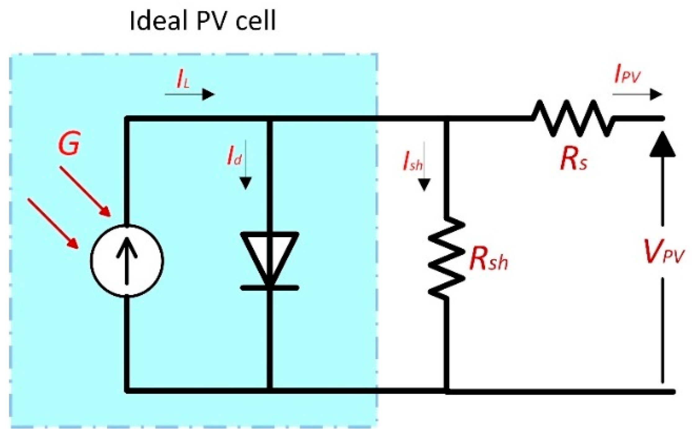
2.2. Modelling of PV Generation

In this section, the modelling of a PV system is proposed, which consists of a PV cell that is converting the irradiance of sunlight into power based on a photon-voltage effect. The ideal cell is connected with series and shunt resistances to present the factors of magnitude resistance and the non-optimal PN junction diode of the PV semiconductor, as shown in Figure 3. Kirchhoff’s current law is used to find its current generation, as shown in Equation (21):

$${\mathit{I}}_{\mathit{P}\mathit{V}}={\mathit{I}}_{\mathit{L}}-{\mathit{I}}_{\mathit{d}}-{\mathit{I}}_{\mathit{s}\mathit{h}}$$

(21)

The current load of the PV diode is given in Equation (22):

$${\mathit{I}}_{\mathit{L}}=\mathit{G}\left\{{\mathit{I}}_{\mathit{S}\mathit{C}}\left[\mathbf{1}+\mathit{k}\mathit{a}\left(\mathit{T}-{\mathit{T}}_{\mathit{S}\mathit{T}\mathit{C}}\right)\right]\right\}$$

(22)

while the reviser current of the PV diode is given by Shockley’s equation (Equation (23)):

$${\mathit{I}}_{\mathit{d}}={\mathit{I}}_{\mathbf{0}}\left\{\mathbf{exp}\left(\frac{ \mathit{q}{\mathit{V}}_{\mathit{d}} }{\mathit{n}\mathit{k}\mathit{T}}\right)-\mathbf{1} \right\}$$

(23)

Finally, a general equation of the PV cell circuit is presented in Equation (24):

$${\mathit{I}}_{\mathit{P}\mathit{V}}={\mathit{I}}_{\mathit{L}}-{\mathit{I}}_{\mathbf{0}}\left[ \mathbf{exp}\left(\frac{ \mathit{q}\left({\mathit{V}}_{\mathit{P}\mathit{V}}+\mathit{I} {\mathit{R}}_{\mathit{S}}\right)}{\mathit{n}\mathit{k}\mathit{T}}\right)-\mathbf{1} \right]-\left[\frac{{\mathit{V}}_{\mathit{P}\mathit{V}}+\mathit{I} {\mathit{R}}_{\mathit{S}}}{{\mathit{R}}_{\mathit{s}\mathit{h}}}\right]$$

(24)

A PV module is created by connecting many PV cells in series and parallel to generate the required current and voltage from a PV system. The output power of a PV system totally depends on the irradiance of the sun and the temperature. To model a PV system with a hybrid power grid, the transfer function of a PV model with a derivative state-space equation is represented by Equation (10) [25]:

$${\mathit{G}}_{\mathit{P}\mathit{V}}\left(\mathit{S}\right)=\frac{{\mathit{K}}_{\mathit{P}\mathit{V}}}{{\mathit{T}}_{\mathit{P}\mathit{V}}\mathit{S}+\mathbf{1}}$$

(25)

where K_PV is the gain of PV generation and T_PV is the time constant of the PV system. The main nomenclatures of PV generation are presented in

Table 2. Nomenclatures of PV generation.

Parameters	Definition
IPV	Output PV current
IL	Current generator
I0	Saturation current
q	Electrical charge
n	PV diode factor
k	Boltzmann’s constant
T	Ambient temperature
VPV	Output PV voltage
Rs	Series resistance
Rsh	Shunt resistance

.

A diagram of a hybrid power system is presented in Figure 4. In the simulation of a hybrid power system, the PV generation is connected with a classical power system as a second source because it has more unpredictable power generation when compared with other renewable energies.

3. Materials and Methods

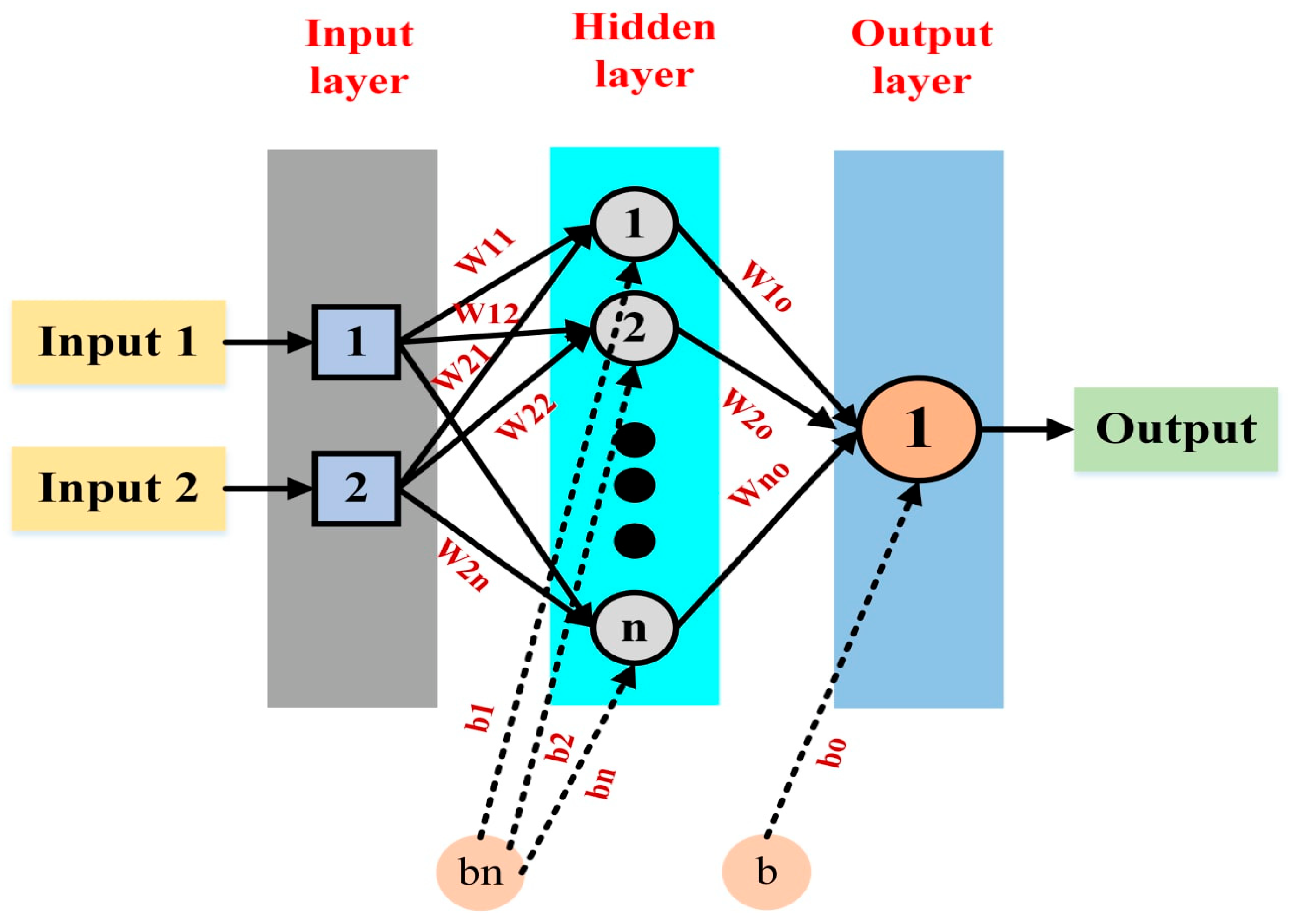
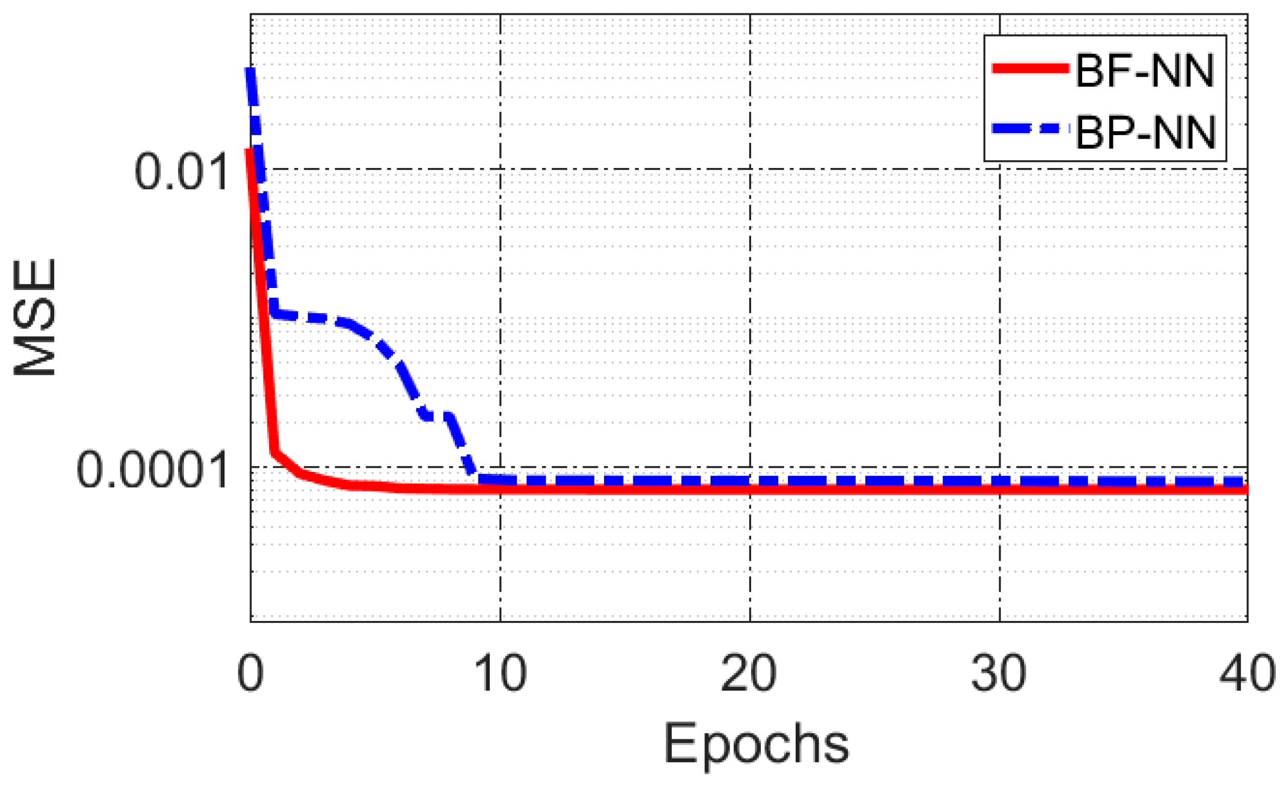
3.1. Neural Network Technique

An NN technique is usually used in industrial applications to predict a precise indication based on handling mechanisation data regarding the practical variables of an operation system [30,31]. There are two types of NN models, feedforward NN and feedback NN, which are classified based on the topology of NN nodes. The first type is considered more often since it requires less memory and training data [32]. In addition, it has a strong capacity to identify the ideal weighting layer [33]. The structure of an NN model consists of three layers, the input layer, hidden layer, and output layer, as shown in Figure 5. They are connected through the weights and biases of nodes, which are calculated mathematically using Equation (26):

$${\mathit{s}}_{\mathit{j}}={\displaystyle \sum }_{\mathit{i}=\mathbf{1}}^{\mathit{n}}{\mathit{w}}_{\mathit{i}\mathit{j}}{\mathit{x}}_{\mathit{j}}+\mathit{b}\mathit{j}$$

(26)

where x_j is the input signal, $w_{ij}$ is the weights, $b_j$ is the biases, and n represents the number of input signals. To learn the values of these nodes, a back-propagation (BP) algorithm is frequently used by changing the values based on Equation (27):

$${\mathit{w}}_{\mathit{j}\mathit{i}}^{\mathit{l}}\left(\mathit{t}\right)=\mathit{\eta }{\mathit{w}}_{\mathit{j}\mathit{i}}^{\mathit{l}}\left(\mathit{t}-\mathbf{1}\right)+\mathit{\mu } \Delta {\mathit{w}}_{\mathit{j}\mathit{i}}^{\mathit{l}}\left(\mathit{t}\right)$$

(27)

where $w_{ji}^l\left(t\right)$ is the present training weight and $w_{ji}^l\left(t-1\right)$ is the antecedent training weight, while $\eta$ is the learning rate and $\mu$ is the grading vector. A sigmoid activation function is utilised as a threshed signal, which is presented mathematically in Equation (28):

$$\mathit{f}\left(\mathit{s}\right)=\frac{\mathbf{1}}{\mathbf{1}+{\mathit{e}}^{-\mathit{s}\mathit{j}}}$$

(28)

This learning continues until the nodes of the NN model are distributed according to the training data. In each step, the predicting signal of the NN (Tj(i)) and actual value of the training data (Yj(i)) are calculated mathematically based on the equation of the mean squared error (MSE), as depicted in Equation (29):

$$\mathit{M}\mathit{S}\mathit{E}=\frac{\mathbf{1}}{\mathit{n}}{\displaystyle \sum }_{\mathit{i}=\mathbf{1}}^{\mathit{n}}{\displaystyle \sum }_{\mathit{j}=\mathbf{1}}^{\mathit{m}}{\left[{\mathit{Y}}_{\mathit{j}}\left(\mathit{i}\right)-{\mathit{T}}_{\mathit{j}}\left(\mathit{i}\right)\right]}^{\mathbf{2}}$$

(29)

where m is the number of output signals. Identifying the most exemplary weights for the learning nodes is the important step to enhance the prediction of the NN model since it finds a low MSE value quickly.

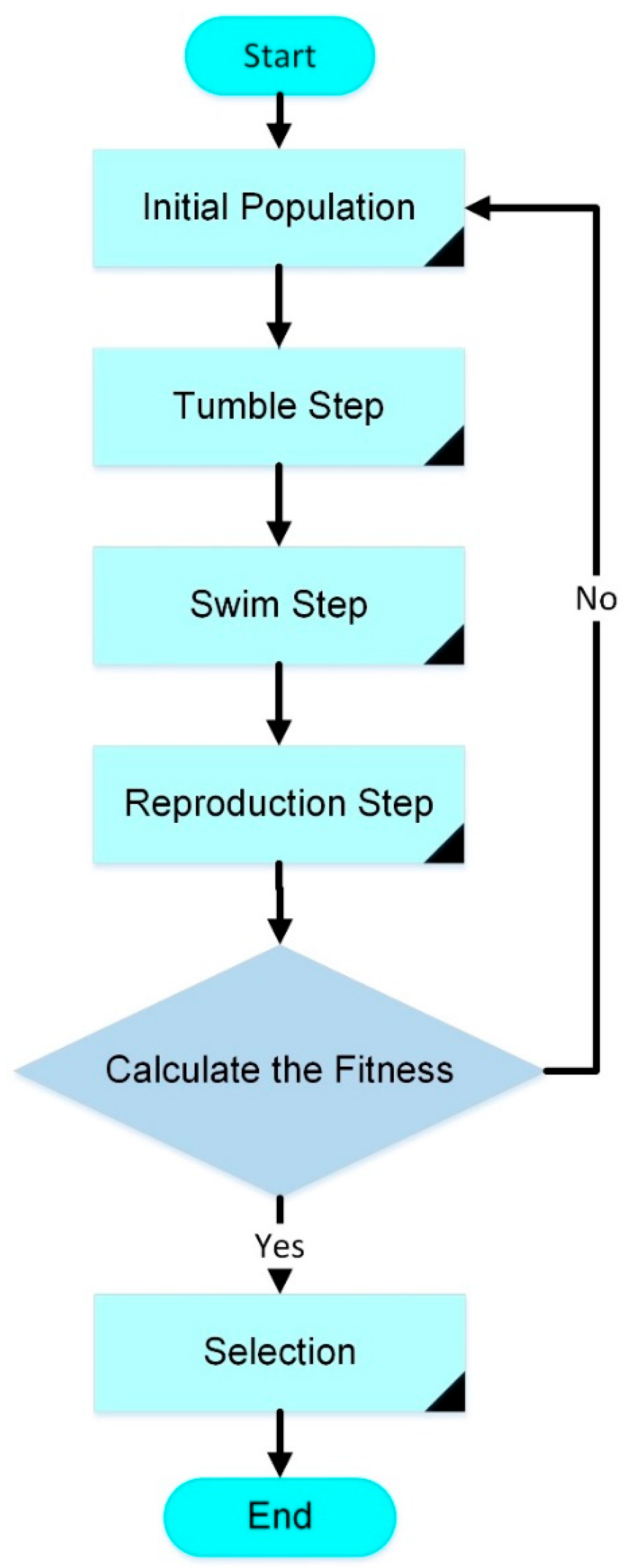
3.2. Bacterial Foraging Algorithm

The BF algorithm was evaluated by Passino in 2002 based on the movement of bacteria when they search for a good location with food [34]. It is usually used in industrial applications to find the accurate parameters of an optimal design with the minimum total solution space, achieving a faster convergence when compared with the classical research algorithms such as PSO, BP, and the genetic algorithm (GA) [35,36,37,38,39,40]. In a process system, the technique divides into four parts, chemotaxis, swarming, reproduction, and elimination and dispersal, as explained in Figure 6.

A.

Chemotaxis Step

In this stage, the bacteria search for food by swimming and tumbling using flagella. The flagellum of each bacterium moves in one direction to swim or in different directions, which results in swanning or tumbling movements, to research the best location for food. These movements are modelled mathematically using Equation (30):

$${\mathit{\theta }}^{\mathit{i}}\left(\mathit{j}+\mathbf{1},\mathit{k},\mathit{l}\right)={\mathit{\theta }}^{\mathit{i}}\left(\mathit{j},\mathit{k},\mathit{l}\right)+\mathit{C}\left(\mathit{i}\right)\varnothing \left(\mathit{j}\right)$$

(30)

where ${\theta }^i\left(j+1,k,l\right)$ represents the bacterium size at the chemotactic step, which is taken in the random direction specified by the tumble loop, while $C\left(i\right) \mathrm{and} \varnothing \left(j\right)$ represent the forward swimming step size and the unit direction vector, respectively.

B.

Swarming Step

In the second step, bacteria try to find the best location for food by searching the optimal way when they signal to other bacteria to swarm together in the right position. Hence, they crowd into different groups based on the accurate path of the food location. This process is represented mathematically by Equation (31):

$${\mathit{J}}_{\mathit{C}}\left(\mathit{\theta },\mathit{P}\left(\mathit{j},\mathit{k},\mathit{l}\right)\right)={\displaystyle \sum }_{\mathit{i}=\mathbf{1}}^{\mathit{s}}{\mathit{J}}_{\mathit{c}}^{\mathit{i}}\left(\mathit{\theta },{\mathit{\theta }}^{\mathit{i}}\left(\mathit{j},\mathit{k},\mathit{l}\right)\right)$$

(31)

where $J_C\left(\theta ,P\left(j,k,l\right)\right)$ represents a time-varying cost function that is presented by adding the cost function value to the real cost function, which must be reduced, while “S” is the total number of bacteria and “p” is the quantity of variables in each bacterium that need to be improved.

C.

Reproduction Step

In this step, the groups of bacteria divide into two major groups based on healthy bacteria and the healthiest bacteria, which have the minimum standard error. The first group of bacteria die, while the second group of bacteria grow in the same location. Therefore, the population size of the bacteria becomes constant duration this step. The number of bacteria in this step is calculated using Equation (32):

$${\mathit{J}}_{\mathit{h}\mathit{e}\mathit{a}\mathit{l}\mathit{t}\mathit{h}}^{\mathit{i}}={\displaystyle \sum }_{\mathit{j}=\mathbf{1}}^{{\mathit{N}}_{\mathit{C}}}\mathit{J}\left(\mathit{i},\mathit{j},\mathit{k},\mathit{l}\right)$$

(32)

where Nc represents the number of chemotactic steps.

D.

Elimination and Dispersal Step

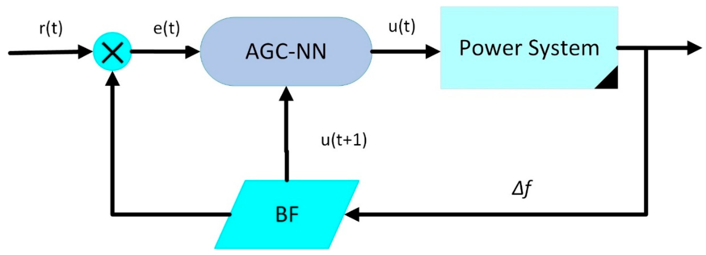
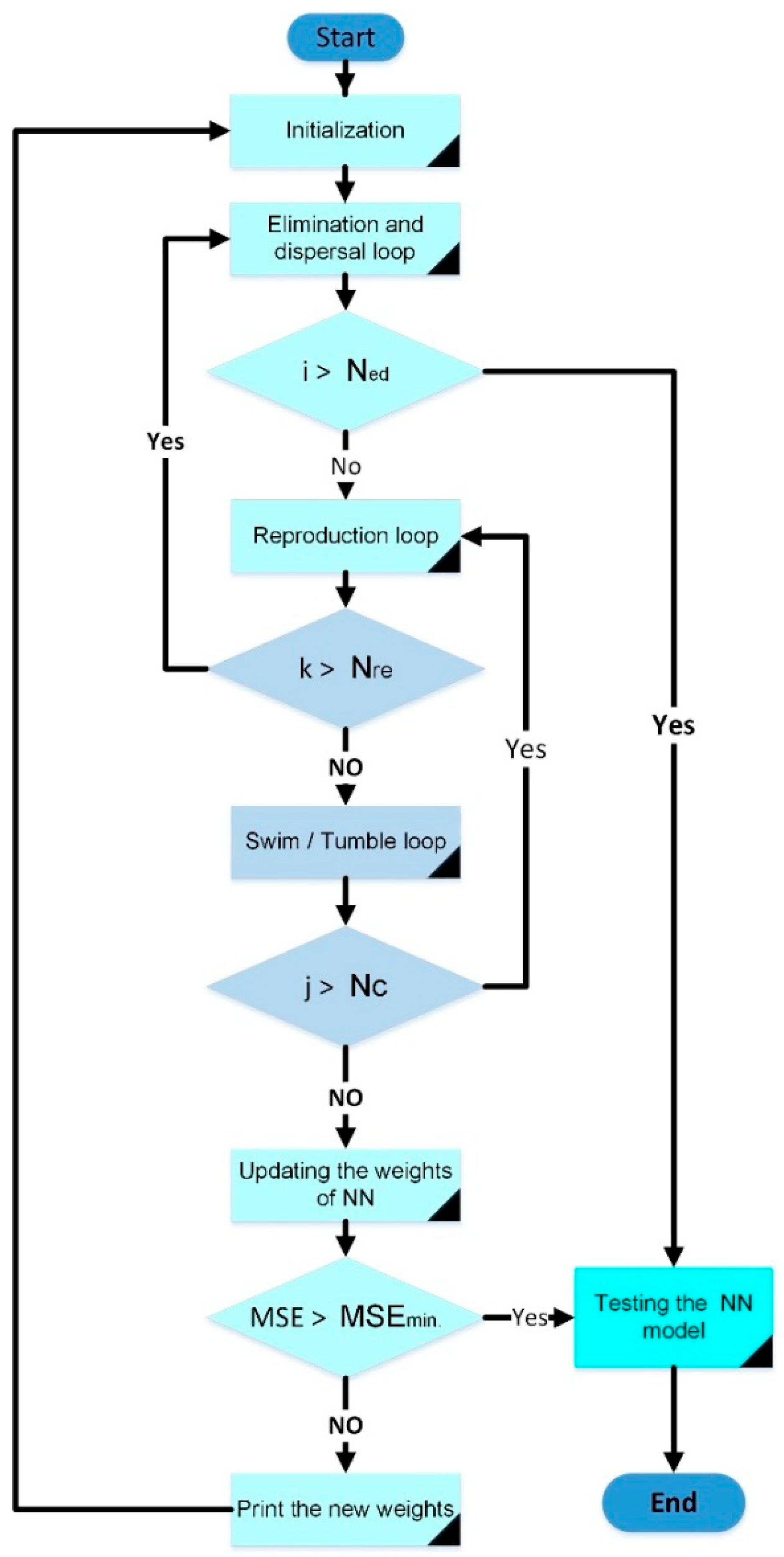
In real life, a small group of bacteria lives due to the surrounding environment. Therefore, they start to gradually change their location based on the consumption of nutrients. During this process, the chemotactic progress of living bacteria is eliminated. Conversely, the chemotaxis of bacteria assists in dispersing living bacteria to a nearby location that has a good food source. These new positions of the healthiest bacteria are adjusted as the current best positions. This process is continued for each of the healthiest bacteria until completing the life cycles of bacteria to determine the best value among them, which is considered the best solution.

4. Proposed Method

As mentioned earlier, identifying the primary weights for the learning nodes is an important step to regulate the performance of the NN model since it finds a low MSE value quickly. However, the BP algorithm usually fails to address the ideal initial weights based on Equation (27). This happens when the value of $\Delta W$ is large and may lead to swift learning with a large step, resulting in a non-converged ideal enhancement. In contrast, small step weights may lead to belated learning with a low step, resulting in stopping the enhancement of the NN model before it identifies the minimum error. In this work, the ideal initial weights were identified based on the BF algorithm because it strongly converges with research on the right solutions with the minimum time compared to the classical research algorithms.

Initially, the training data for the historical change in the frequency response and the type of power disturbance were collected from the standard Simulink of a power system. Ten thousand samples were collected from the standard power system to train the PF-NN model, as proposed in Figure 7. Then, the training data were optimised using the hybrid BF-NN algorithm, as shown in Figure 8. Its main parameters are explained in

Table 3. Parameters of BF-NN algorithm.

Parameters	Value
Dimension of search space	93
Bacterial size (S)	50
Number of chemotactic steps (Nc)	5
Number of reproduction steps (Nre)	50
Number of elimination/dispersal events (Ned)	4
Probability of eliminated/dispersed	0.25

. It printed out the ideal initial weights after it trained the NN model for several steps. In each step, it checked the value of MSE until the ideal initial weights were addressed. Next, the NN model was trained using the “nn-tool” command of MATLAB. Hence, the MSE of the BF-NN model reached a minimum value of 3 × 10⁻⁴ in epoch 11, while the MSE of the BP-NN model reached about 9 × 10⁻⁴ in epoch 40, as shown in Figure 9. Finally, the proposed model was employed with an AGC for a two-area power system with grid-connected PV generation. The input of the AGC was the error in the historical change in the frequency response with tie-line power, while the output was the signal of the governor. The AGC optimisation base on the PF algorithm aimed to find the accurate parameters of the optimal design with the minimum total solution space, achieving a faster convergence when compared with the classical research algorithms, such as the BP algorithm.

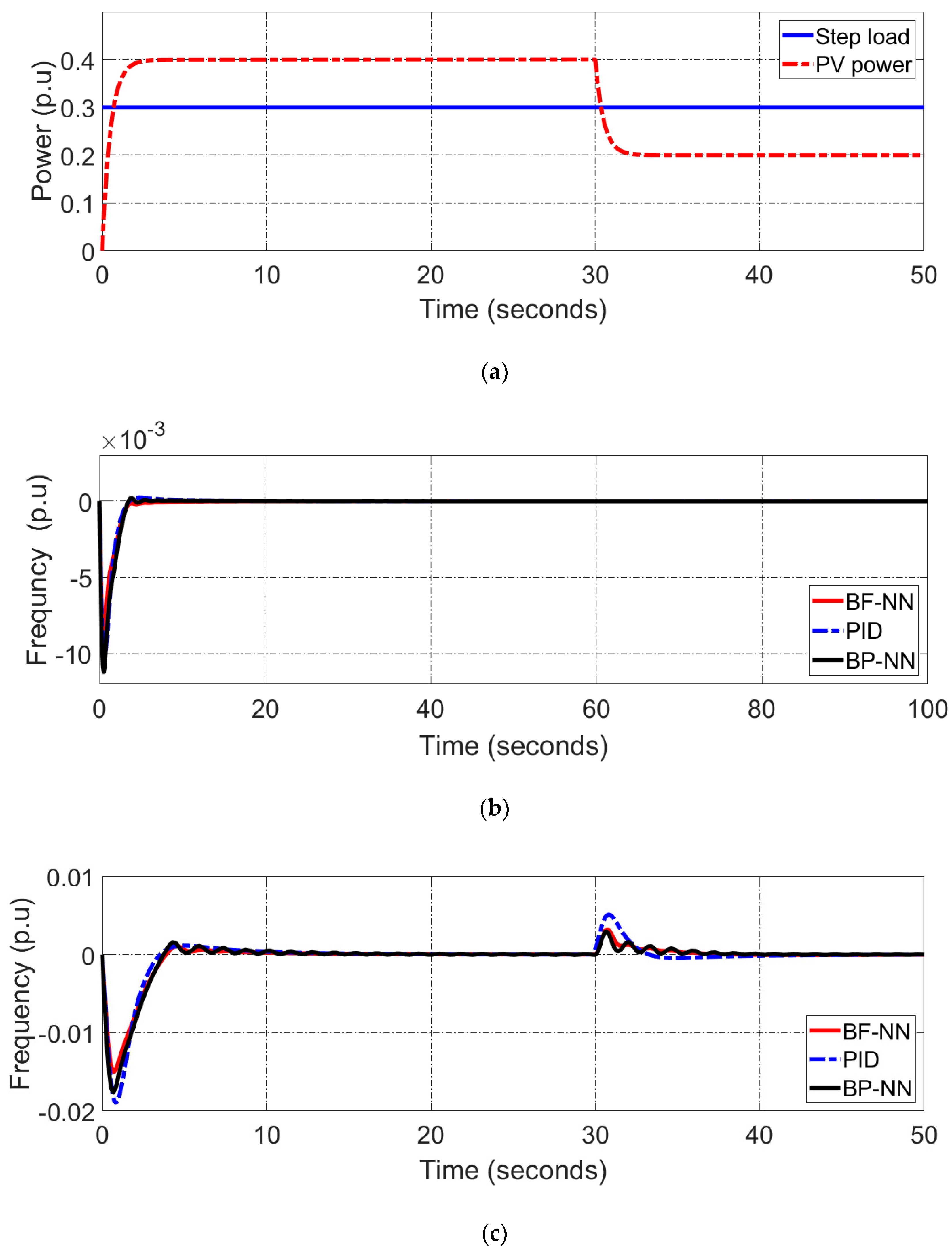
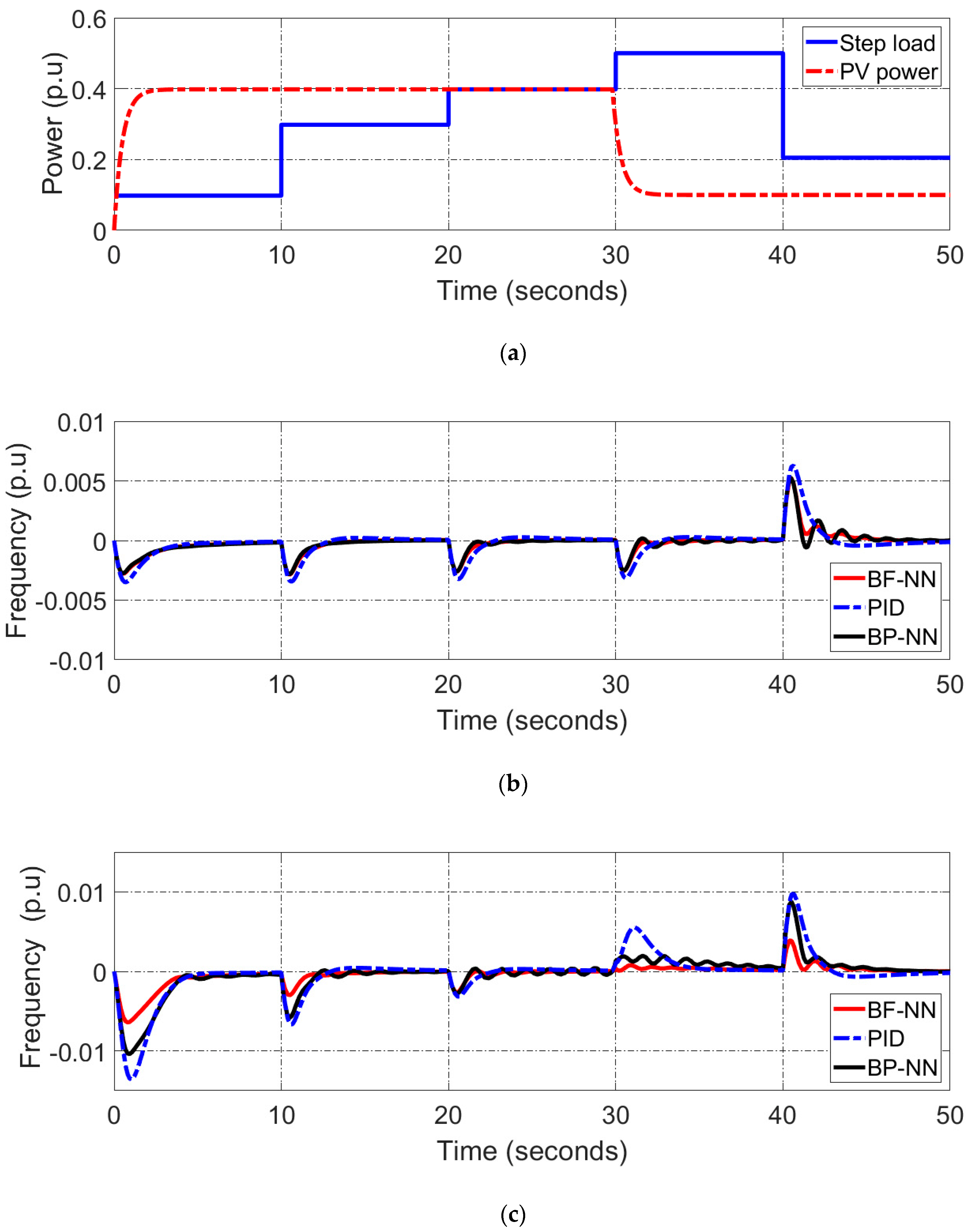
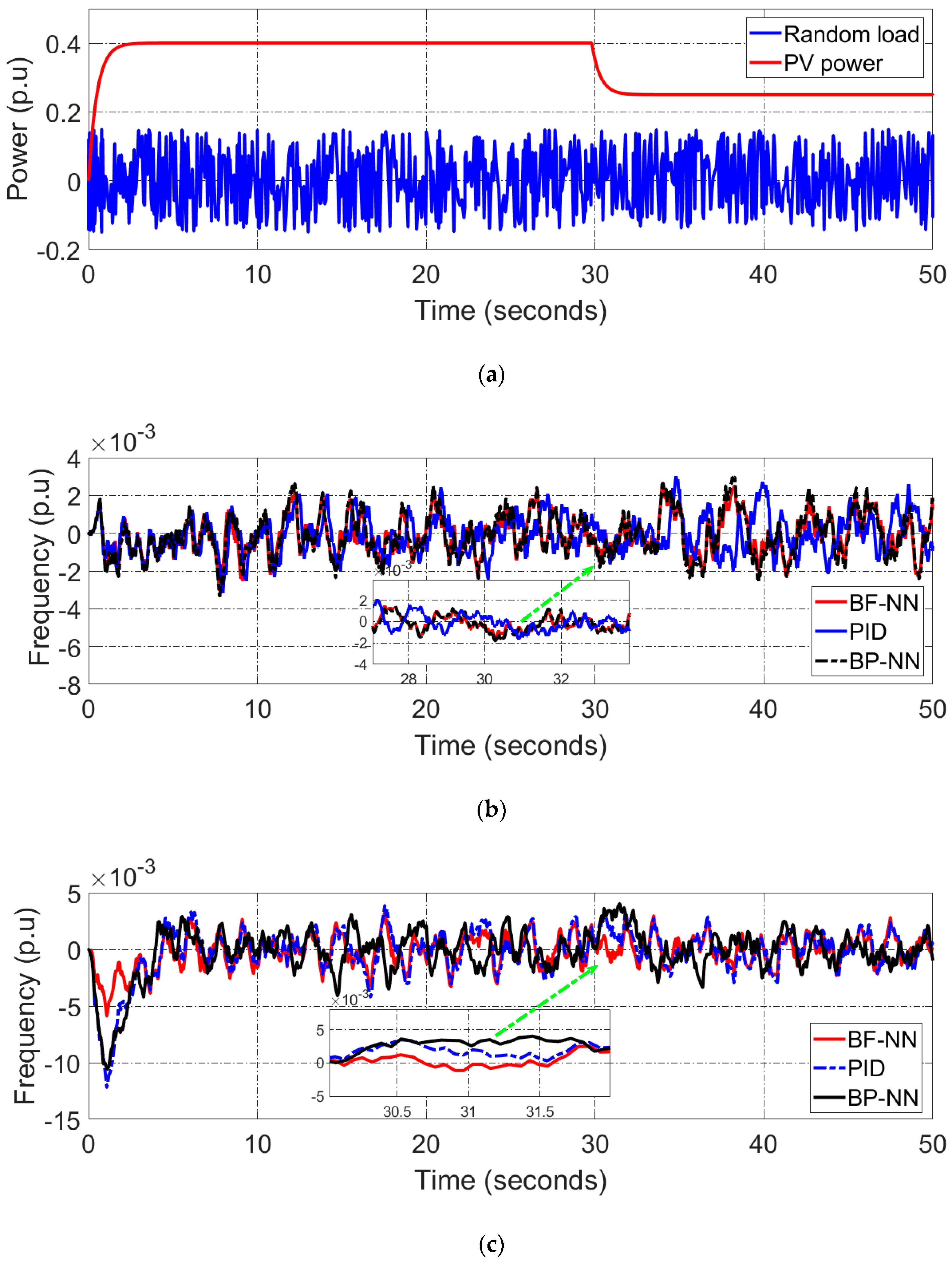
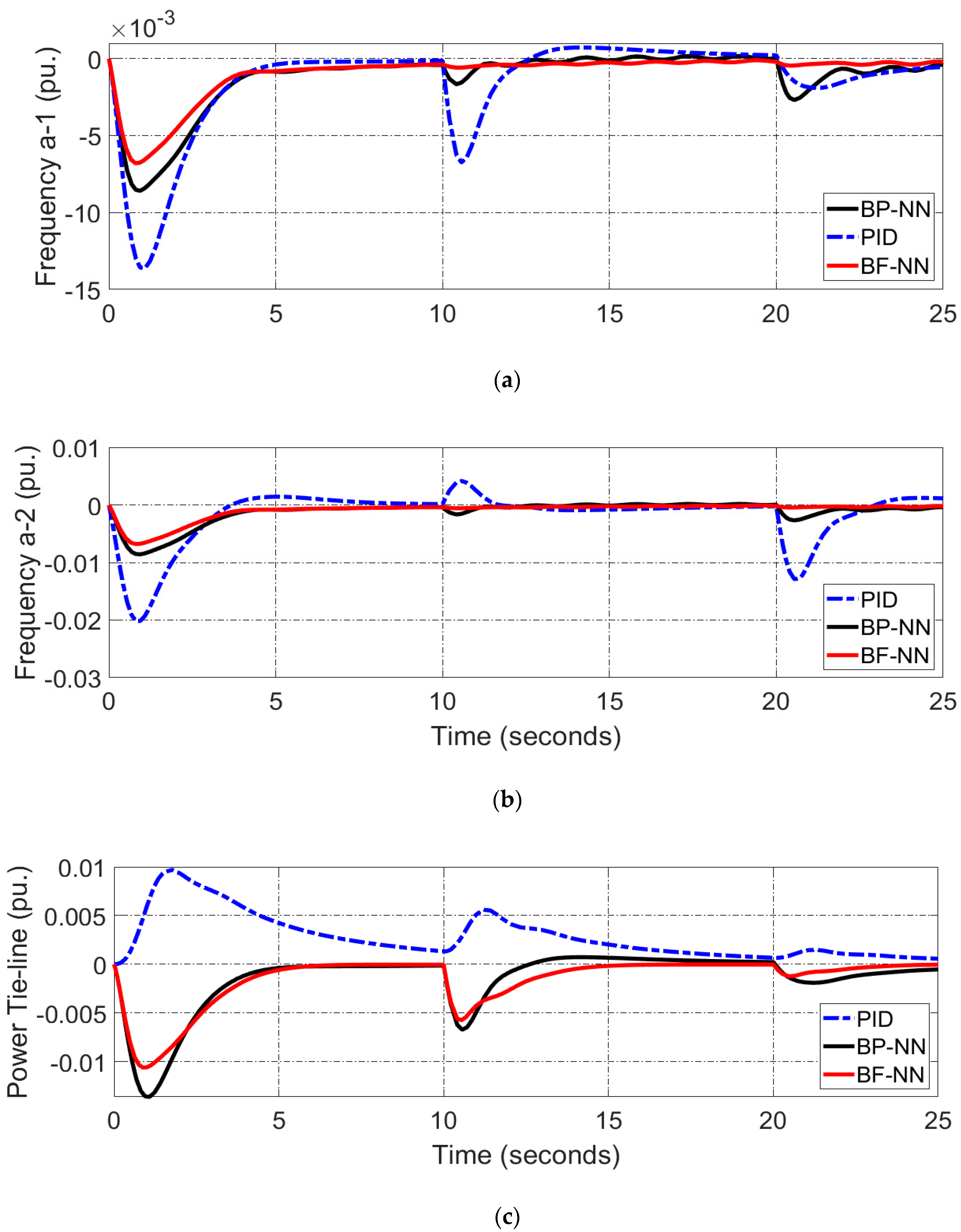
5. Results and Discussion

To assess the proposed PF-ANN method, a hybrid power system was designed with a grid-connected PV source based on an AGC for two areas. It was compared with the conventional BP-NN and PID approaches. The main parameters of the Simulink model for the hybrid power system were the 100 MW output power of the two areas; the 0.5 pu. and 0.6 pu. speed regulation of the governors for areas 1 and 2, respectively; the 0.2 s and 0.3 s time constants of the governors for areas 1 and 2, respectively; the 4 s and 5 s inertia constants of generators for areas 1 and 2, respectively; the 0.6 and 0.9 frequencies of the sensitive load coefficient for areas 1 and 2, respectively; the 20 Hz and 16.9 Hz frequency base factors for areas 1 and 2, respectively; and the 0.5 s time constant of PV generation. The proposed AGC was tested according to four cases as follows: an initial operation condition with and without PV generation, a load-changing disturbance for various times with and without PV generation, a fault condition with and without PV generation, and an operation condition for the two-area hybrid power system. The PV generation was considered during variable conditions such as partial shading, variable irradiance, and variable temperature, which impact the output power of a PV system.

Case 1: In the first case, the load changed from 0% to 30% in the initial operation, while the PV generation changed from 40% to 20% at 30 s, as shown in Figure 10a. It can be seen that the proposed AGC was the most reliable to reset the frequency response of the power system to zero with PV generation and without PV generation compared to the NN-AGC and PID-AGC, as seen in Figure 10b. In addition, it minimised the overshoot of the frequency response when the PV generation changed at 30 s, as depicted in Figure 10c. However, the transient time in the hybrid power system was greater compared with the transient time of the conventional power system due to the unpredictable power of the PV source.

Case 2: In the second case, the AGC based on the hybrid PF-NN method was tested under variable load disturbances at different times without and with the same PV generation as in case one, as illustrated in Figure 11a. During this time, the proposed method offset the frequency deviation to zero for the entire periodical test, although the oscillation continued more than in case one, as shown in Figure 11b. Moreover, it was the better dynamic to address the decrease in the load demand at 40 s when the PV generation decreased since the overshoot of the frequency was minimised and it reduced the transient time compared with the BP-NN and PID controllers, as presented in Figure 11c.

Case 3: In the third case, a fault condition test was designed to adequately assess the validation of the proposed method. The fault condition was designed based on the random value of the power amplitude of 0.05 pu. and the scale variation of the frequency response of 50 rad/second, while the PV generation changed from 40% to 25% at 40 s. In comparison to the BP-NN and PID approaches under various state conditions, the AGC based on the BF-NN was the most precise for finding the frequency level of the hybrid power system. It was relatively close to zero error deviation, as shown in the Figure 12, and its zoom point was clearer. However, the frequency response did not reach zero, specifically on the negative side, due to an unbalanced state.

Case 4: Finally, the proposed method was tested for the two-area power system in the same condition state as in case 1, which was the case with PV generation. It was noticed that the frequency responses of area 1 and area 2 of the hybrid power system were able to avoid mismatching in the load demand when they were changed nonlinearly at various times, as presented in Figure 13a,b. Moreover, the power of the tie-line system for the proposed AGC was mostly stable, while the tie-line power of the BP-NN-AGC and the PID-AGC drifted from the zero point, as shown in Figure 13c.

Lastly, an integral of time-multiplied absolute error (ITAE) formula was used to test the proposed AGC method numerically (33) [16]:

$$\mathit{I}\mathit{T}\mathit{A}\mathit{E}={{\displaystyle \int }}_{\mathbf{0}}^{{\mathit{t}}_{\mathit{s}\mathit{i}\mathit{m}}}(\left|\Delta {\mathit{f}}_{\mathbf{1}}\right|+\left|\Delta {\mathit{f}}_{\mathbf{2}}\right|+\left|\Delta {\mathit{P}}_{\mathit{t}\mathit{i}\mathit{e}}\right|.\mathit{t}.\mathit{d}\mathit{t}$$

(33)

where $\Delta f_1$ and $\Delta f_2$ are the historical change in the frequencies of area 1 and area 2, respectively, and $\Delta P_{tie}$ is the total power of the two-area hybrid power system. Based on this determination, the proposed method reached a steady-state error at 5.20 s under various condition states, while the BP-NN and PID of the AGC achieved the ITAE at 8.79 s and 13.25 s, respectively, as illustrated in

Table 4. ITAE for BF-NN, BP-NN, and PID approaches.

Approaches	ITAE
BF-NN	5.20 s
BP-NN	8.79 s
PID	13.25 s

. This was due to the proposed method’s reduced MSE to accurately predict the signal in a condensed processing time.

6. Conclusions

A BF algorithm was applied to enhance the learning of a neural network model for the automatic generation controller of a hybrid power system. It addressed the identical initial weights of the NN quickly. To sum up, ten thousand samples of training data were collected for the hybrid power system. Then, they were learned by the BF-NN model for several tests. Hence, the training error of the BF-NN model reached a minimum value of about 3 × 10⁻⁴ in 11 epochs, compared to the training error of the BP-NN algorithm, which stopped at about 9 × 10⁻⁴ after 40 epochs. Next, the proposed AGC was tested according to four cases: an initial operation condition with and without PV generation, a load-changing disturbance for various times with and without PV generation, a fault condition with and without PV generation, and an operation condition for the two-area hybrid power system. The results showed that the algorithm offset the frequency diversion, minimised the overshoot, and reduced the transit time of the hybrid power system in the four condition states. Moreover, it achieved the lowest standard transit time of about 5.20 s, while the BP-NN and PID approaches were extended to 8.79 s and 13.25 s, respectively. In future work, an experimental hybrid power system network will be tested.

References

1. Feng, W.; Xie, Y.; Luo, F.; Zhang, X.; Duan, W. Enhanced stability criteria of network-based load frequency control of power systems with time-varying delays. Energies 2021, 14, 5820. [Google Scholar] [CrossRef]
2. Chen, B.Y.; Shangguan, X.C.; Jin, L.; Li, D.Y. An improved stability criterion for load frequency control of power systems with time-varying delays. Energies 2020, 13, 2101. [Google Scholar] [CrossRef] [Green Version]
3. Ma, M.; Liu, X.; Zhang, C. LFC for multi-area interconnected power system concerning wind turbines based on DMPC. IET Gener. Transm. Distrib. 2017, 11, 2689–2696. [Google Scholar] [CrossRef]
4. Al-Majidi, S.D.; Al-Nussairi, M.K.; Mohammed, A.J.; Abbod, M.F.; Al-raweshidy, H.S. Design of a Load Frequency Controller Based on an Optimal Neural Network. Energies 2022, 15, 6223. [Google Scholar] [CrossRef]
5. Ranjan, M.; Shankar, R. A literature survey on load frequency control considering renewable energy integration in power system: Recent trends and future prospects. J. Energy Storage 2022, 45, 103717. [Google Scholar] [CrossRef]
6. Tan, W.; Zhang, H.; Yu, M. Decentralized load frequency control in deregulated environments. Int. J. Electr. Power Energy Syst. 2012, 41, 16–26. [Google Scholar] [CrossRef]
7. Pappachen, A.; Fathima, A.P. Critical research areas on load frequency control issues in a deregulated power system: A state-of-the-art-of-review. Renew. Sustain. Energy Rev. 2017, 72, 163–177. [Google Scholar] [CrossRef]
8. Alhelou, H.H.; Hamedani-Golshan, M.E.; Zamani, R.; Heydarian-Forushani, E.; Siano, P. Challenges and opportunities of load frequency control in conventional, modern and future smart power systems: A comprehensive review. Energies 2018, 11, 2497. [Google Scholar] [CrossRef] [Green Version]
9. Yang, M.; Wang, C.; Hu, Y.; Liu, Z.; Yan, C.; He, S. Load frequency control of photovoltaic generation-integrated multi-area interconnected power systems based on double equivalent-input-disturbance controllers. Energies 2020, 13, 6103. [Google Scholar] [CrossRef]
10. Sitharthan, R.; Karthikeyan, M.; Sundar, D.S.; Rajasekaran, S. Adaptive hybrid intelligent MPPT controller to approximate effectual wind speed and optimal rotor speed of variable speed wind turbine. ISA Trans. 2019, 96, 479–489. [Google Scholar] [CrossRef]
11. Sitharthan, R.; Geethanjali, M. An adaptive Elman neural network with C-PSO learning algorithm-based pitch angle controller for DFIG based WECS. J. Vib. Control 2015, 23, 716–730. [Google Scholar] [CrossRef]
12. Soundarya, G.; Sitharthan, R.; Sundarabalan, C.K.; Balasundar, C.; Karthikaikannan, D.; Sharma, J. Design and Modeling of Hybrid DC/AC Microgrid With Manifold Renewable Energy Sources. IEEE Can. J. Electr. Comput. Eng. 2021, 44, 130–135. [Google Scholar] [CrossRef]
13. Pandey, S.K.; Kishor, N.; Mohanty, S.R. Frequency Regulation in Hybrid Power System Frequency Regulation in Hybrid Power System Using Iterative Proportional-Integral-Derivative H∞. Electr. Power Compon. Syst. 2014, 42, 132–148. [Google Scholar] [CrossRef]
14. Bevrani, H.; Member, S.; Feizi, M.R.; Member, S. Robust Frequency Control in an Islanded Microgrid: H∞ and μ-Synthesis Approaches. IEEE Trans. Smart Grid 2016, 7, 706–717. [Google Scholar] [CrossRef] [Green Version]
15. Shayeghi, H.; Shayanfar, H.A.; Jalili, A. Load frequency control strategies: A state-of-the-art survey for the researcher. Energy Convers. Manag. 2009, 50, 344–353. [Google Scholar] [CrossRef]
16. Chen, G.; Li, Z.; Zhang, Z.; Li, S. An Improved ACO Algorithm Optimized Fuzzy PID Controller for Load Frequency Control in Multi Area Interconnected Power Systems. IEEE Access 2020, 8, 6429–6447. [Google Scholar] [CrossRef]
17. Grigsby, L.L. Power System Stability and Control, 3rd ed.; CRC Press: Boca Raton, FL, USA, 2017; pp. 1–450. [Google Scholar] [CrossRef]
18. Zhong, Q.; Yang, J.; Shi, K.; Zhong, S.; Li, Z.; Sotelo, M.A. Event-Triggered Load Frequency Control for Multi-Area Nonlinear Power Systems Based on Non-Fragile Proportional Integral Control Strategy. IEEE Trans. Intell. Transp. Syst. 2022, 23, 12191–12201. [Google Scholar] [CrossRef]
19. Al-Majidi, S.D.; Abbod, M.F.; Al-Raweshidy, H.S. Maximum Power Point Tracking Technique based on a Neural-Fuzzy Approach for Stand-alone Photovoltaic System. In Proceedings of the UPEC 2020-2020 55th International Universities Power Engineering Conference, Torino, Italy, 1–4 September 2020. [Google Scholar] [CrossRef]
20. Al-Majidi, S.D.; Abbod, M.F.; Al-Raweshidy, H.S. Design of an Efficient Maximum Power Point Tracker Based on ANFIS Using an Experimental Photovoltaic System Data. Electronics 2019, 8, 858. [Google Scholar] [CrossRef] [Green Version]
21. Sa-ngawong, N.; Ngamroo, I. Intelligent photovoltaic farms for robust frequency stabilization in multi-area interconnected power system based on PSO-based optimal Sugeno fuzzy logic control. Renew. Energy 2015, 74, 555–567. [Google Scholar] [CrossRef]
22. Al-Nussairi, M.K.; Al-Majidi, S.D.; Hussein, A.R.; Bayindir, R. Design of a Load Frequency Control based on a Fuzzy logic for Single Area Networks. In Proceedings of the 10th IEEE International Conference on Renewable Energy Research and Application (ICRERA 2021), Ankara, Turkey, 26–29 September 2021; pp. 216–220. [Google Scholar] [CrossRef]
23. Karimipouya, A.; Abdi, H. Microgrid frequency control using the virtual inertia and ANFIS-based Controller. Int. J. Ind. Electron. Control Optim. 2019, 2, 145–154. [Google Scholar] [CrossRef]
24. Dash, K.S.R.S.S. Load frequency control of autonomous power system using adaptive fuzzy based PID controller optimized on improved sine cosine algorithm. J. Ambient Intell. Humaniz. Comput. 2018, 10, 2361–2373. [Google Scholar] [CrossRef]
25. Nitisha, K.N.; Puneet, T.; Vineet, M.; Rana, K.K.P.S. Efficient control of integrated power system using self-tuned fractional-order fuzzy PID controller. Neural Comput. Appl. 2018, 31, 4137–4155. [Google Scholar] [CrossRef]
26. Sharma, Y.; Saikia, L.C. Electrical Power and Energy Systems Automatic generation control of a multi-area ST—Thermal power system using Grey Wolf Optimizer algorithm based classical controllers. Int. J. Electr. Power Energy Syst. 2015, 73, 853–862. [Google Scholar] [CrossRef]
27. Kant, S.; Mohanty, S.R.; Kishor, N.; Catalão, J.P.S. Electrical Power and Energy Systems Frequency regulation in hybrid power systems using particle swarm optimization and linear matrix inequalities based robust controller design. Int. J. Electr. Power Energy Syst. 2014, 63, 887–900. [Google Scholar] [CrossRef]
28. Fan, W.; Hu, Z.; Veerasamy, V. PSO-Based Model Predictive Control for Load Frequency Regulation with Wind Turbines. Energies 2022, 15, 8219. [Google Scholar] [CrossRef]
29. El-fergany, A.A.; El-hameed, M.A. Efficient frequency controllers for autonomous two-area hybrid microgrid system using social-spider optimiser. IET Gener. Transm. Distrib. 2017, 11, 637–648. [Google Scholar] [CrossRef]
30. Al-dunainawi, Y.; Abbod, M.F.; Jizany, A. Engineering Applications of Arti fi cial Intelligence A new MIMO ANFIS-PSO based NARMA-L2 controller for nonlinear dynamic systems. Eng. Appl. Artif. Intell. 2017, 62, 265–275. [Google Scholar] [CrossRef] [Green Version]
31. Abdolrasol, M.G.M.; Hussain, S.M.S.; Ustun, T.S.; Sarker, M.R.; Hannan, M.A.; Mohamed, R.; Ali, J.A.; Mekhilef, S.; Milad, A. Artificial neural networks based optimization techniques: A review. Electronics 2021, 10, 2689. [Google Scholar] [CrossRef]
32. Rosa, J.P.S.; Guerra, D.J.D.; Horta, N.C.G.; Martins, R.M.F.; Lourenço, N.C.C. Overview of Artificial Neural Networks; Springer: Berlin/Heidelberg, Germany, 2020. [Google Scholar] [CrossRef]
33. Jain, A.K.; Mao, J.; Mohiuddin, K.M. Artificial neural networks: A tutorial. Computer 1996, 29, 31–44. [Google Scholar] [CrossRef] [Green Version]
34. Al-hadi, I.A.A.; Zaiton, S.; Hashim, M.; Mariyam, S.; Shamsuddin, H. Bacterial Foraging Optimization Algorithm For Neural Network Learning Enhancement. In Proceedings of the 2011 11th International Conference on Hybrid Intelligent Systems (HIS), Melacca, Malaysia, 5–8 December 2011; pp. 200–205. [Google Scholar] [CrossRef]
35. Nanda, J.; Mishra, S.; Saikia, L.C. Maiden Application of Bacterial Foraging-Based Optimization Technique in Multiarea Automatic Generation Control. IEEE Trans. Power Syst. 2009, 24, 602–609. [Google Scholar] [CrossRef]
36. Tang, J.; Liu, G.; Pan, Q. A Review on Representative Swarm Intelligence Algorithms for Solving Optimization Problems: Applications and Trends. IEEE/CAA J. Autom. Sin. 2021, 8, 1627–1643. [Google Scholar] [CrossRef]
37. Eslami, M.; Shareef, H.; Mohamed, A.; Khajehzadeh, M. PSS and TCSC Damping Controller Coordinated Design Using GSA. Energy Procedia 2012, 14, 763–769. [Google Scholar] [CrossRef] [Green Version]
38. Eslami, M.; Shareef, H.; Mohamed, A. Optimization and Coordination of Damping Controls for Optimal Oscillations Damping in Multi-Machine Power System. Int. Rev. Electr. Eng. 2011, 6, 1984–1993. [Google Scholar]
39. Eslami, M.; Neshat, M. A Novel Hybrid Sine Cosine Algorithm and Pattern Search for Optimal Coordination of Power System Damping Controllers. Sustainability 2022, 14, 541. [Google Scholar] [CrossRef]
40. Eslami, M.; Shareef, H.; Mohamed, A.; Khajehzadeh, M. Damping Controller Design for Power System Oscillations Using Hybrid GA-SQP y. Int. Rev. Electr. Eng 2010, 6, 888–896. [Google Scholar]
Figure 1. A schematic diagram of power generation.
Energies 16 02802 g001
Figure 2. Modelling of two-area power system.
Energies 16 02802 g002
Figure 3. Equivalent circuit of PV cell.
Energies 16 02802 g003
Figure 4. Diagram of a hybrid power system.
Energies 16 02802 g004
Figure 5. Structure of an NN model.
Energies 16 02802 g005
Figure 6. Flowchart of a BF algorithm.
Energies 16 02802 g006
Figure 7. Training process of BF-NN model.
Energies 16 02802 g007
Figure 8. Flowchart of a BF-NN algorithm.
Energies 16 02802 g008
Figure 9. Training test of BP-NN vs. BF-NN.
Energies 16 02802 g009
Figure 10. Division signals in an initial operating state of (a) input power, (b) output frequency without PV generation, and (c) output frequency with PV generation.
Energies 16 02802 g010
Figure 11. Division signals in a variable operating state of (a) input power, (b) output frequency without PV generation, and (c) output frequency with PV generation.
Energies 16 02802 g011
Figure 12. Division signals in a fault condition state of (a) input power, (b) output frequency without PV generation, and (c) output frequency with PV generation.
Energies 16 02802 g012
Figure 13. Division signals of a two-area hybrid power system in a mismatching operation state of (a) the output frequency of area 1, (b) the output frequency of area 2, and (c) the tie-line power with PV generation.
Energies 16 02802 g013