Electric Vehicle Charging Hub Power Forecasting: A Statistical and Machine Learning Based Approach

Abstract

Electric vehicles (EVs) penetration growth is essential to reduce transportation-related local pollutants. Most countries are witnessing a rapid development of the necessary charging infrastructure and a consequent increase in EV energy demand. In this context, power demand forecasting is an essential tool for planning and integrating EV charging as much as possible with the electric grid, renewable sources, storage systems, and their management systems. However, this forecasting is still challenging due to several reasons: the still not statistically significant number of circulating EVs, the different users’ behavior based on the car parking scenario, the strong heterogeneity of both charging infrastructure and EV population, and the uncertainty about the initial state of charge (SOC) distribution at the beginning of the charge. This paper aims to provide a forecasting method that considers all the main factors that may affect each charging event. The users’ behavior in different urban scenarios is predicted through their statistical pattern. A similar approach is used to forecast the EV’s initial SOC. A machine learning approach is adopted to develop a battery-charging behavioral model that takes into account the different EV model charging profiles. The final algorithm combines the different approaches providing a forecasting of the power absorbed by each single charging session and the total power absorbed by charging hubs. The algorithm is applied to different parking scenarios and the results highlight the strong difference in power demand among the different analyzed cases.

1. Introduction

Current policies of the European Union and national governments are strongly pushing the transition to local zero-emission mobility based on electric vehicles (EVs). This is being followed by continued growth in the number of circulating electric vehicles. Therefore, we are witnessing a rapid and widespread development of the necessary charging infrastructure. The simultaneous global push toward energy transition leads to accompanying the installation of charging systems with the installation of photovoltaic and storage systems for optimal energy management. This is making demand forecasting an essential topic of strong interest.

On one hand, for the charging infrastructure providers, the forecasting of user energy consumption is essential to estimate possible revenues and losses to assess the cost-effectiveness of the installations [1,2]. On the other hand, for the grid operators, the forecasting of the power required for EV charging is mandatory to quantify the effects on the power grid management and stability [3,4,5,6]. Predicting the EV charge power profiles allows effective charging management strategies [7] and the optimal integration of EVs with the electrical grid, storage systems, and renewable sources [8,9,10,11].

However, power forecasting in this context is still challenging due to several reasons. The current number of EVs is still statistically not representative to derive a robust model based on the available data [12]. Moreover, despite the general continuous growth, in some countries like Italy, the number of new EV registrations is experiencing an unexpected decrease [13]. Added to this is the fact that, the charging power profile is highly dependent on many different factors. The power level of the charging can vary in a wide range. The most common value is 22 kW for AC charging points (CPs) [14], but it can reach hundreds of kW in the DC stations [15]. However, the effective use of the available power level can vary among the different EV manufacturers and models [16]. For example, the Renault ZOE can charge up to 46 kW in DC, while the Renault Twingo cannot exceed the 22 kW exclusively in the AC mode. The Tesla Model Y can achieve a 250 kW DC peak power during the charge. Eventually, this power level is not constant during the whole charging process. The charge of lithium batteries is typically carried out by means of the constant current-constant voltage (CC-CV) charging protocol [17]. This protocol involves a reduction in the charging power during the final stage of charging to preserve the state of health of the battery. For this reason, the resulting power profile is discontinuous. Moreover, the profile of absorbed power varies in relation to many other factors such as the battery technology, the onboard charger, or the adopted battery management system [18].

In the case of charging hubs (CHs), the whole absorbed power profile is in turn dependent on many other factors related to the considered scenario and the users’ behavior. The arrival times distribution of a CH of a working place parking lot typically presents a peak around the first-morning hours while, in a CH of a shopping area, this peak typically occurs around the evening. Finally, the energy demand of each CH is influenced by other factors like the state of charge (SOC) of the battery at the beginning of the charge, and the duration of parking (i.e., the time the CP remains occupied).

Several works about EV charging parameters forecasting can be found in the literature. Authors in [19] adopted Bayesian inference methods with convolution to forecast the daily charging pattern of an EV fleet. This work only considers the 3 kW household power level, then results can not be applied to public CH in different parking lot scenarios, charging station power levels, and EV models. A day-ahead Bayesian deep learning forecasting method was proposed in [20]. The objective was to capture the uncertainties in EV charging forecasting by adopting Bayesian theory and neural networks. In [21], a forecasting method based on multi-source data and prospect theory was presented. The travel behaviour of private electric vehicles and taxi owners was considered along with the roads’ velocity and network. Authors in [22] compared four different deep learning methods for a real case in Marocco to predict charging demand of an EV station. In [23], a data-driven approach using machine learning regression methods is adopted for a public charging station. In [24], historical data was clustered based on EV user behaviour and the corresponding probability density functions were derived. Three main parameters were considered, i.e., arrival time, charging duration and average power. These works, which are mainly based on charging data analysis, don’t provide a method able to take into account the single session charging power as a function of the time. Moreover, charging infrastructure and EV characteristics (such as initial/final state of charge, maximum power capability, battery capacity etc.) were not considered. Finally, authors in [8] provide a forecasting method based on a statistical model of the arrival and departure time of the users. Although this method calculates the power consumed by each connected vehicle as a function of time, only 22 kW AC charging points are considered, and only a single parking scenario (i.e., a metal-working company) was analyzed. To the best of authors’ knowledge no papers provide a charging forecasting method based on specific EV and CH infrastructure characteristics, different urban scenarios, and real charging power profiles.

The proposed work aims to fill this gap at both single charging point and total charging hub level by considering multiple approaches. The users’ behavior is modeled through a statistical-based approach in which arrivals, departures, and charging durations are predicted based on the specific patterns related to the considered scenario. The distribution of the EV battery SOCs at the beginning of the charge is based on a probabilistic analysis of specific consumption and distances traveled before the charging event of each vehicle. A machine-learning-based approach is used to develop a battery charging behavioral model (BCBM). The BCBM is able to emulate the charging power profile of different EV models as a function of the battery SOC and the power rating of the CP to which the EV is connected. Based on custom input settings that describe the CH charging station characteristics, the expected number of EVs, and the operating scenario, the resulting forecasting algorithm evaluates the charging power profile of each EV and the SOC evolution of each EV during the whole period in which it is connected to the CP with a fine time resolution. Finally, the forecasting algorithm provides as output the total power demand of the CH as a function of the time.

The paper is structured as follows: Section 2 analyzes the main parameters influencing EV charging power demand and provides models to emulate their patterns, trends and behavior; Section 3 describes the prediction algorithm; Section 4 shows and discusses the results of the proposed method by comparing them under different scenarios; Finally, conclusions are drawn in Section 5.

2. Analysis and Modeling of Parameters Influencing EV Charging

The reference scenario object of the study is a generic CH within a car park in which the EV parking lots present a charging point as sketched in Figure 1. EV users can arrive at the CH and depart it at different times of the day.

The total CH power $P_{\mathrm{CH}}$ is assumed equal to the sum of power $P_{\mathrm{EV}}$ provided to each vehicle. The daily power absorption of the CH is computed by taking the following factors under consideration:

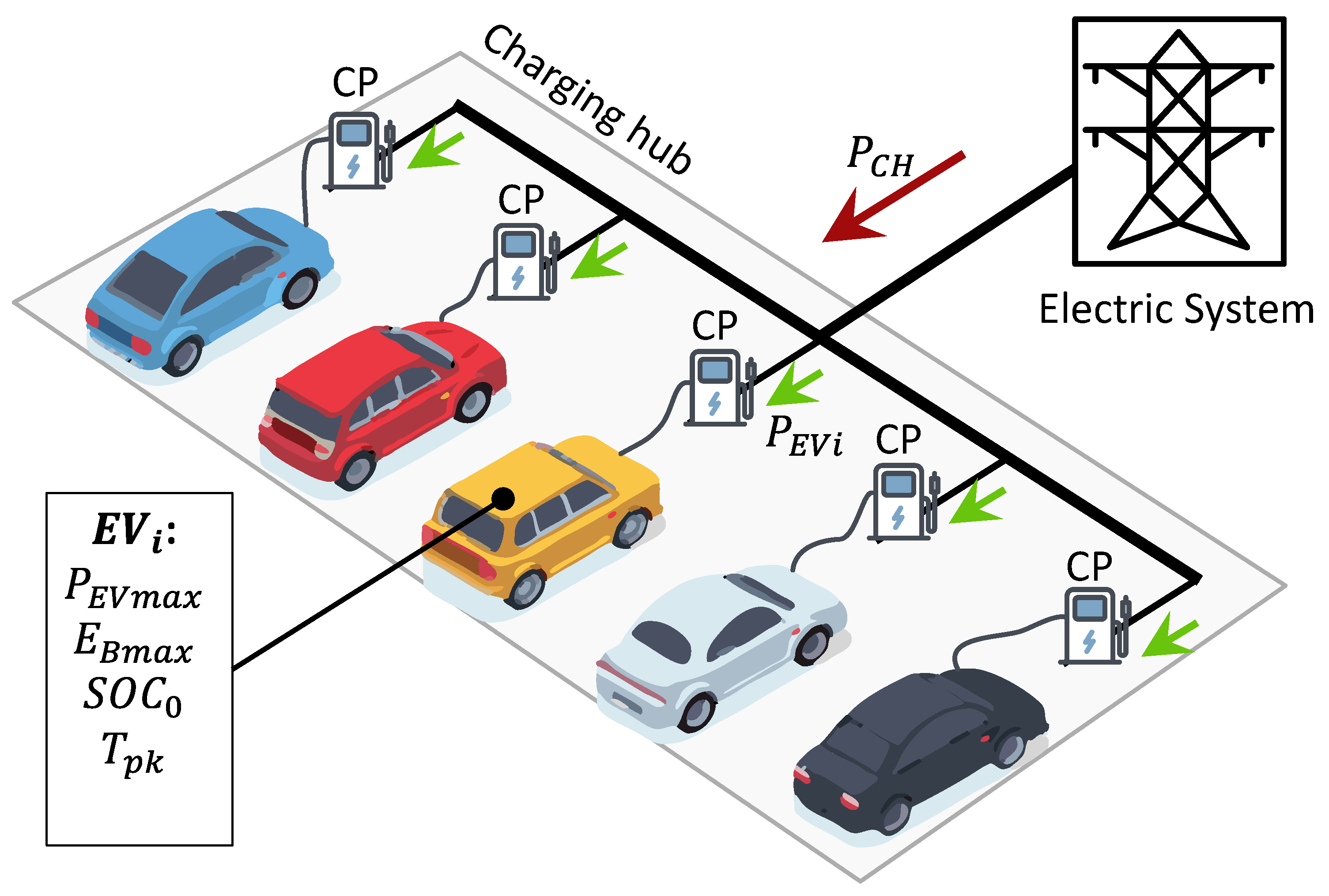
• The maximum power made available by the CP, named $P_{\mathrm{CP}}$ (kW). The CH is considered composed of CP of the same kind.
• The EV characteristics in terms of maximum power $P_{\mathrm{EVmax}}$ accepted by the battery and its maximum capacity $E_{\mathrm{Bmax}}$.
• The EV users’ behavior in terms of arrival and departure times, parking duration ($T_{\mathrm{pk}}$), and charging duration.
• The initial state of charge ($SO{C}_0$), i.e., the SOC value at the arrival of the EV at the parking lot, that depends on the EV users’ behavior and consumption before the charging event.
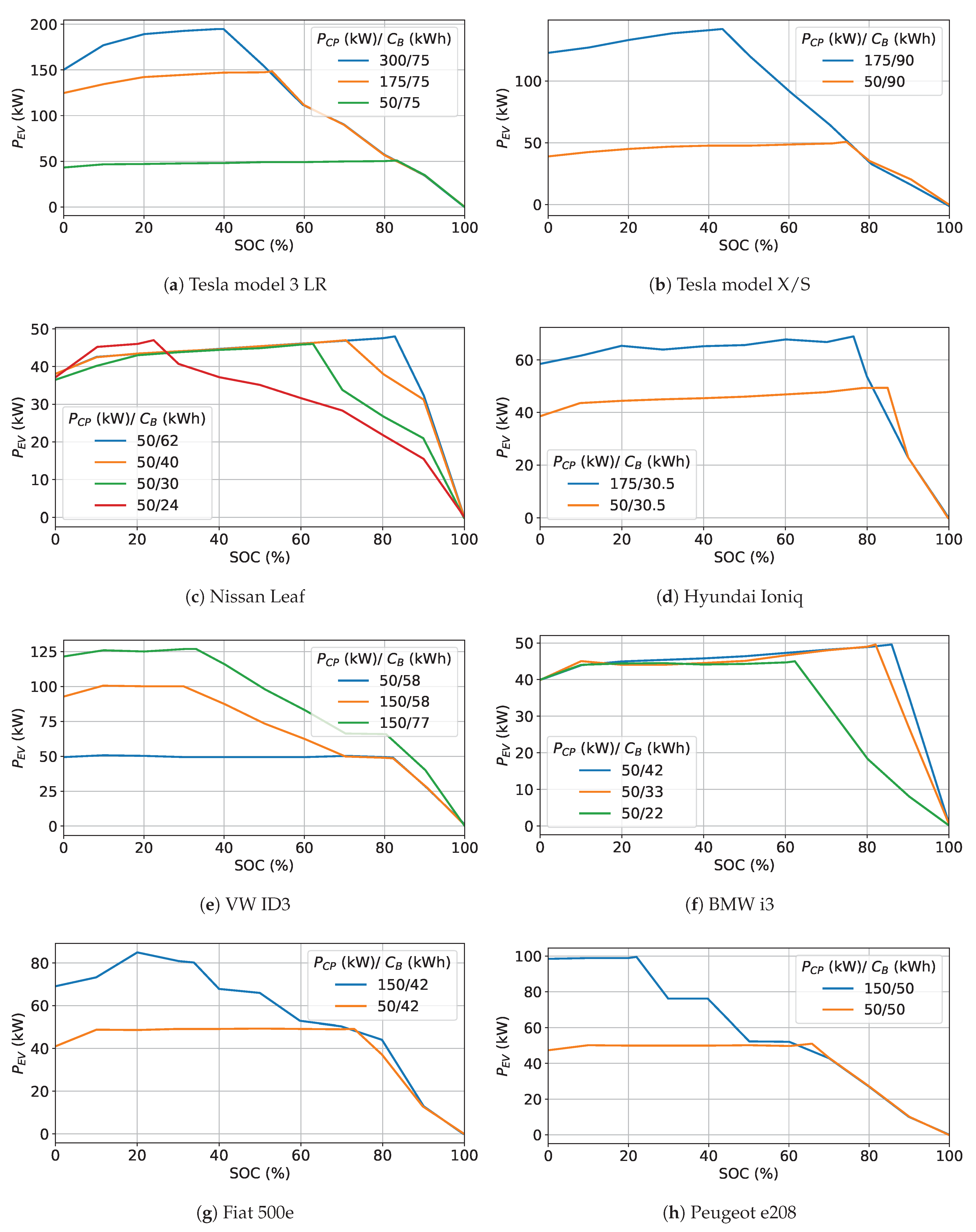
• The profile evolution of the power absorbed by the battery during the charging process in relation to charging station and EV models.

The discussion of each parameter is addressed in detail in the following sections.

2.1. Charging Infrastructure and EV Model Characteristics

According to the EU Alternative Fuels Infrastructure Regulation (AFIR) [25], the charging points are divided into two categories based on the typology of connection between the vehicle and the charging station:

• Category 1. The CP provides an AC output power and the battery charging is managed by the EV on-board charger [26].
• Category 2. The CP provides a DC output power and the battery charging is managed directly by the off-board converter installed inside the charging station [27].

The on-board charger size is limited by the reduced space that is available in the vehicles. Then, the AC CPs generally have a lower power rating than the DC category.

A sub-classification of the EV charging systems considers different output power and the consequent charging speed. This classification system is summarized in

Table 1. Charging point categories based on AFIR Proposal (Annex III) [25].

Category	Sub-Category	Power Output	Definition
	Slow AC charging point, single-phase	$P_{\mathrm{CP}}<7.4\mathrm{kW}$	Normal power
Category 1 (AC)	Medium AC charging point, triple-phase	$7.4\mathrm{kW}\le P_{\mathrm{CP}}\le 22\mathrm{kW}$	Normal power
	Fast AC charging point, triple-phase	$P_{\mathrm{CP}}>22\mathrm{kW}$	High power
	Slow DC charging point	$P_{\mathrm{CP}}<50\mathrm{kW}$	High power
Category 2 (DC)	Fast DC charging point	$50\mathrm{kW}\le P_{\mathrm{CP}}<150\mathrm{kW}$	High power
	Level 1—Ultra-fast DC charging point	$150\mathrm{kW}\le P_{\mathrm{CP}}<350\mathrm{kW}$	High power
	Level 2—Ultra-fast DC charging point	$P_{\mathrm{CP}}\ge 350\mathrm{kW}$	High power

.

The number of charging stations has grown in the past three years, the year 2022 also confirms this growing trend. Figure 2a (data retrieved from [28]) shows a strong increase in AC charging points belonging to the “medium-speed AC” category. The figure also shows that the main increase in the DC category is related to “fast DC” and “ultra-fast DC”—Level 1 systems. Currently, 88% of the CPs in the EU belong to the AC category. The pie-plot in Figure 2b shows that 73% of CPs provide power between $7.4\mathrm{kW}$ and $22\mathrm{kW}$ followed by 11% of CPs having a power rating lower than $7.4\mathrm{kW}$. The DC charging category only provides 11% of the total number of CPs. Most DC CPs have a power rating between $50\mathrm{kW}$ and $150\mathrm{kW}$ (5.5%), followed by ultra-fast charging—Level 1 (3.8%).

Electric vehicle registrations in Europe are growing as well. The number of EVs on the road more than tripled from 616 thousand in 2019 to about 2 million in 2021. However, the EVs share in comparison to the total car fleet still remains very low, at around 0.81% [12].

The different graphs of Figure 3 summarize the characteristics of the 20 best-selling EV models in Italy. Specifically, the abscissa represents the variation range of some features for the EV population considered: the usable battery capacity (a), the specific consumption in terms of $\mathrm{kWh}/100\mathrm{km}$ (b), the AC charging (c) and DC charging (d) power capability. The scatter plot depicts the feature value for each EV model indicated in the y-axis. The markers’ size is proportional to the share of the model on the total number of registered EVs. The histograms, referred to the left-axes, depict the distribution of the corresponding features among the population. The specific consumption data are referred to the world harmonized light-duty vehicles test procedure (WLTP) declared by manufacturers [16]. The reported vehicles represent 90% of the whole registrations in Italy in 2021. Since some of these models have different options for battery capacity and engine size, only the characteristics of the most popular models are considered for the sake of analysis simplification. Finally, the vertical dashed line depicts the average values.

The data analysis allows a baseline of the users of each hypothetical CH. Specifically, the following conclusions can be drawn:

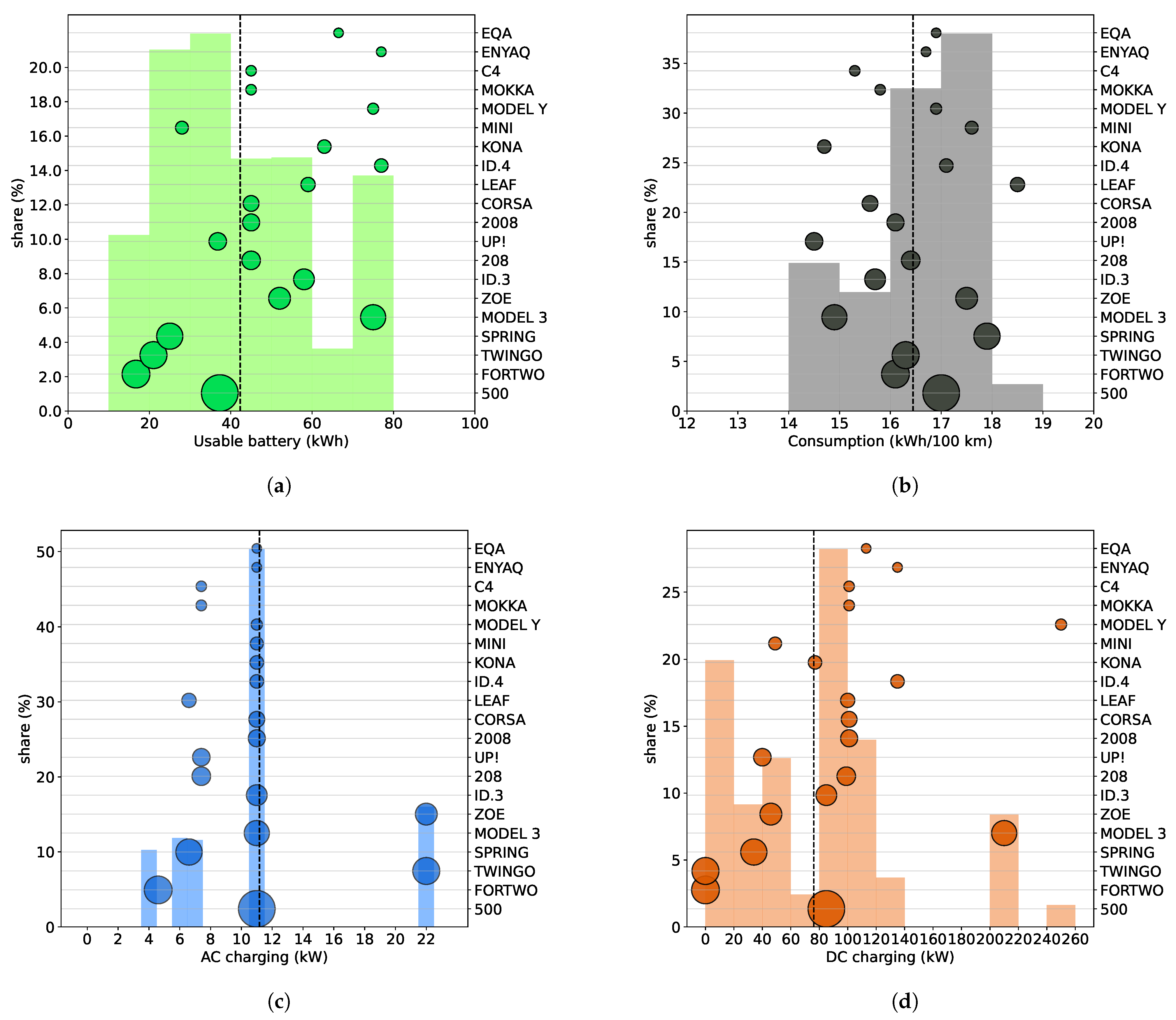
• The average usable battery capacity (Figure 3a) is $42.3\mathrm{kWh}$ with a standard deviation of $18.6\mathrm{kWh}$. 53% of EVs (including the top 4 registered models) have a capacity of less than $40\mathrm{kWh}$. Compared to the European scenario, the Italian fleet has only 13% of EVs belonging to the 70–80 kWh capacity range.
• The average specific consumption is $16.4\mathrm{kWh}$ per $100\mathrm{km}$. As visible in Figure 3b, the distribution is fairly homogeneous among the fleet and owns a standard deviation of 1 kWh/100 km. Considering the average battery capacity, it is possible to calculate the average distance driven in the WLTP condition, which is about $260\mathrm{km}$.
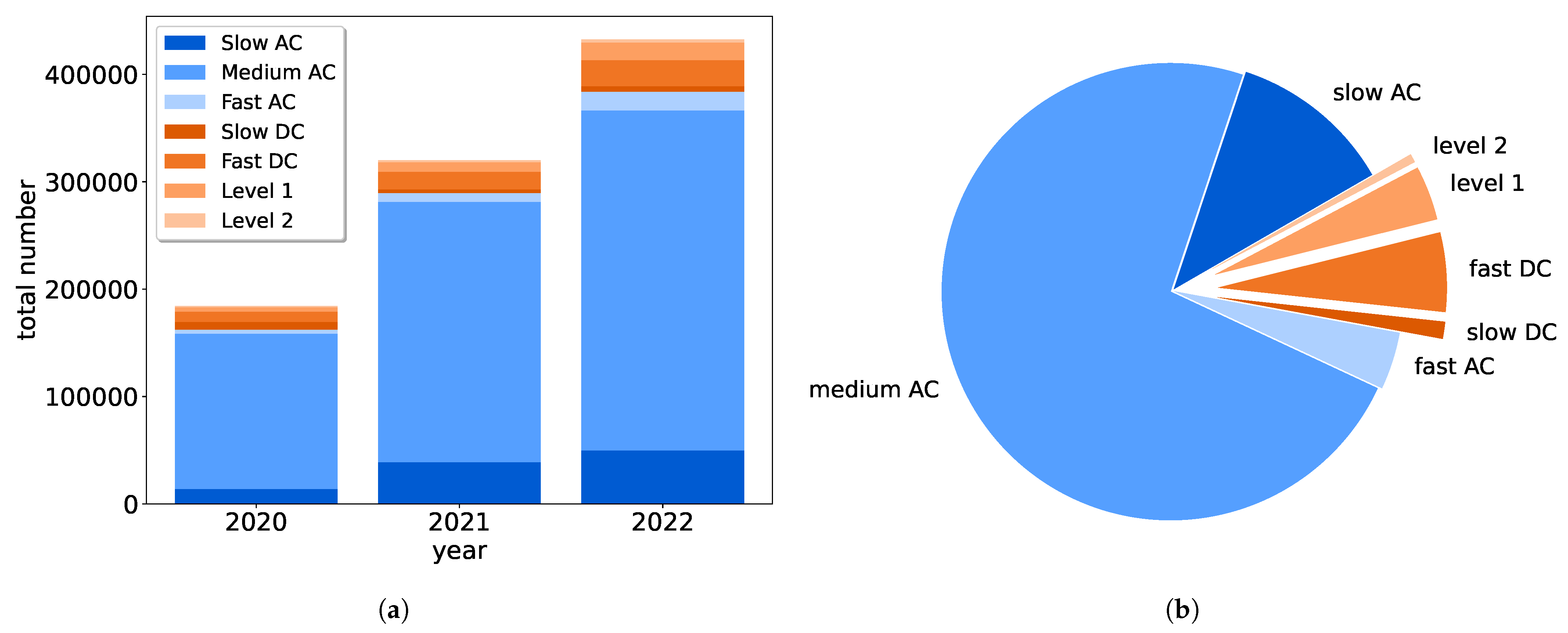
• The average AC charging power (Figure 3c) is equal to $11.16\mathrm{kW}$ with a standard deviation of $5.2\mathrm{kW}$. This value is in line with the European scenario. About 50% of the vehicles have a maximum charging power of $11\mathrm{kW}$. 15% (represented by the Renault brand) can charge up to $22\mathrm{kW}$ in AC. Finally, about 75% of the vehicle’s onboard chargers allow medium-speed AC charging, remaining 25% can only use slow AC levels. No vehicles enable Fast AC charging.
• The average DC charging power (Figure 3d) is $76\mathrm{kW}$ with a standard deviation of $60\mathrm{kW}$. It is worth noting that about 20% of EVs can not charge via DC CP and 20% can only be charged via Slow DC level. About 50% of the fleet can be charged via Fast DC CP. The remaining 10% of EV is enabled to charge via Level 1—Ultra-fast chargers.

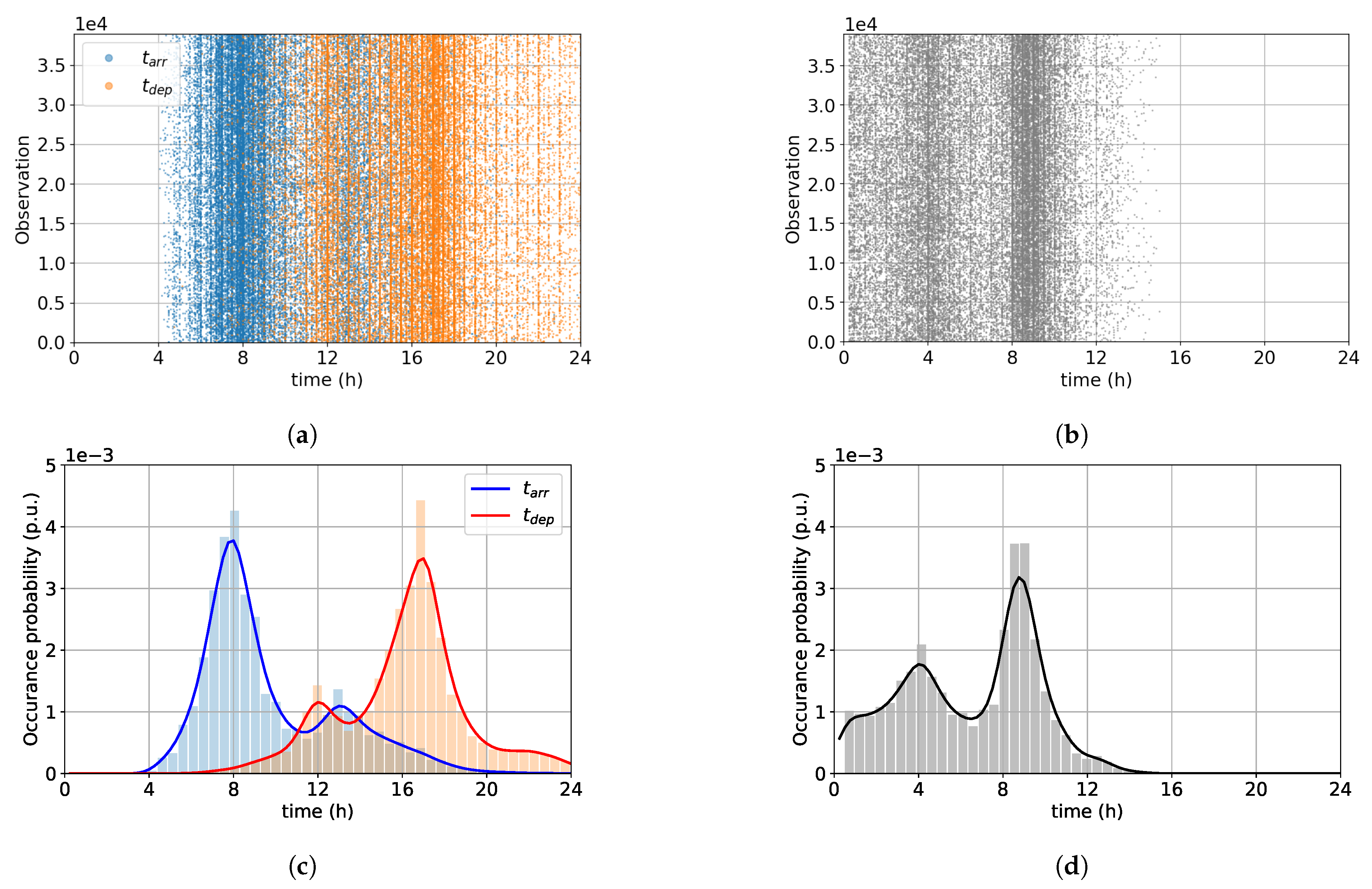
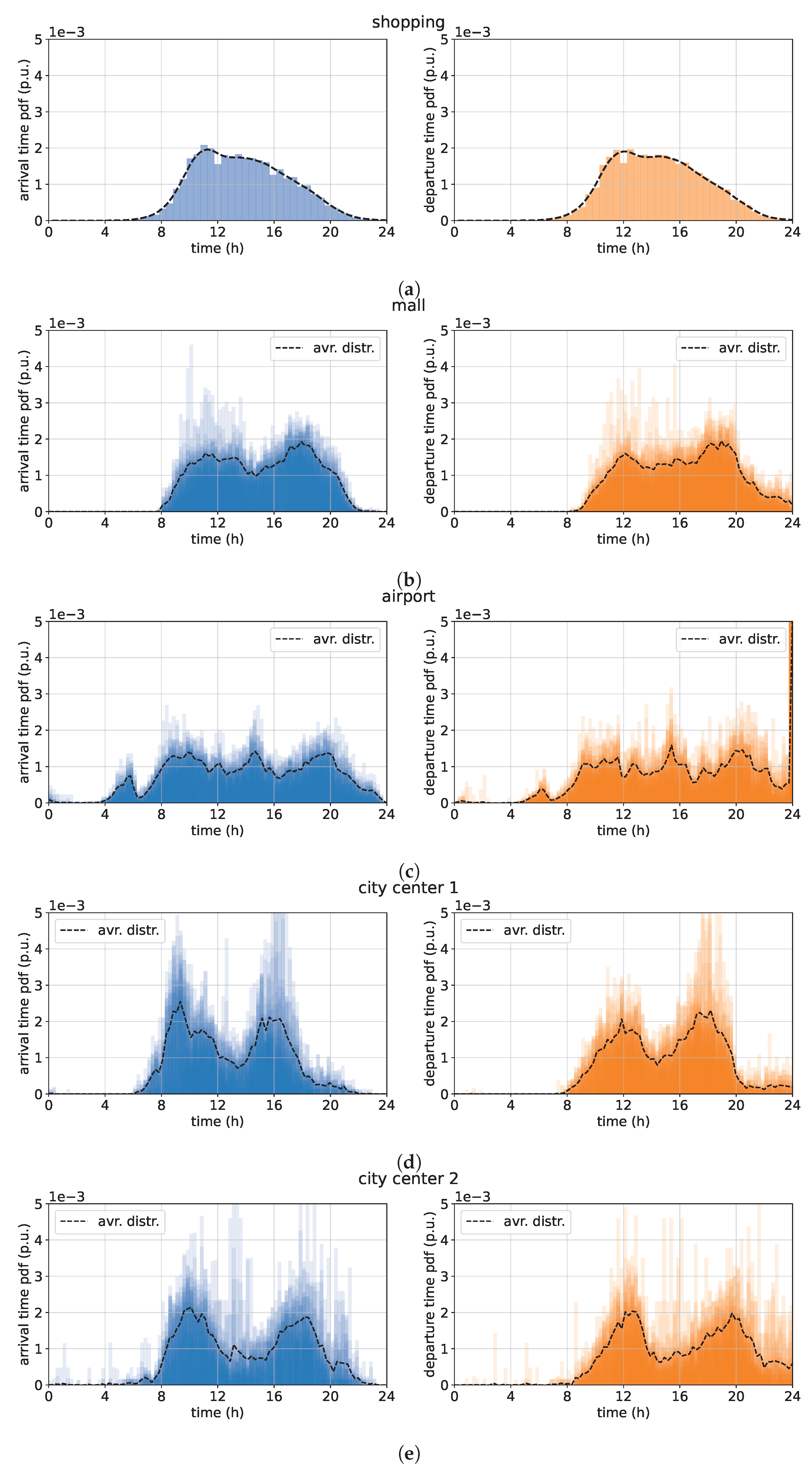
2.2. Statistical Patterns of Users Behavior

This section focuses on the modeling of the users’ behavior in terms of arrival time, departure time, and parking duration. The parking duration $T_{\mathrm{pk}}$ is here defined as:

$${\displaystyle T_{\mathrm{pk}}=t_{\mathrm{dep}}-t_{\mathrm{arr}}}$$

(1)

where $t_{\mathrm{arr}}$ and $t_{\mathrm{dep}}$ are, respectively, the time of arrival and departure of the vehicle at/from the parking lot. The duration of $T_{\mathrm{pk}}$, as well as the instants $t_{\mathrm{arr}}$ and $t_{\mathrm{dep}}$, depend on several factors and change according to the different scenarios in which the CH is located. In order to extrapolate statistical patterns that identify the users’ behavior as a function of the parking lot scenario, two data sources are considered and analysed. The first set of data is derived from the National Household Travel Survey (NHTS) [29]. Some preliminary results are reported in Figure 4 and Figure 5a.

The NHTS presents about one million trip observations. From each observation, it is possible to derive the $t_{\mathrm{arr}}$, the $t_{\mathrm{dep}}$, $T_{\mathrm{pk}}$ associated to a parking scenario and the distance traveled. Through data processing, the main data-set is clustered into two macro scenarios according to the associated reason for travel: motivations related to work activities (named “working scenario”); motivations related to the purchase of services and goods (named “shopping scenario”). The results of the data processing and the statistical pattern obtained are summarized through Figure 4. The scatter plots in Figure 4a,b show the instant of arrival ($t_{\mathrm{arr}}$, blue marker), departure ($t_{\mathrm{dep}}$, orange marker) and parking time of the working scenario users. About 40 thousand observations are collected from [29] and analyzed. The probability density distributions (pdf) pattern derived from the observation are reported in Figure 4c and Figure 4d, respectively. For the working scenario, the $t_{\mathrm{arr}}$ distribution has two peaks, the first around 8:00, and the second around 13:00. The $t_{\mathrm{dep}}$ pdf presents a higher peak around the evening (17:00) and a lower peak at 12:00. Most of the cars are parked for about 9 hours and the average value of $T_{\mathrm{pk}}$ is 6.5 h. Similar analyses are carried out for the shopping scenario data, which statistical pattern of arrival and departure times are reported in Figure 5a. The $t_{\mathrm{arr}}$ and $t_{\mathrm{dep}}$ distributions are found to be similar, concentrated mainly during store opening hours. The average parking time of the shopping scenario is 42 min.

A second analysis is based on data collected from real case studies. A 1-month data collection campaign was carried out on several parking lots located in the urban area of Bologna, in cooperation with companies that provide parking services for EVs. Figure 5 shows the output of data processing in terms of statistical patterns of the car park scenarios. Each figure considers 31 different histograms (normalized) corresponding to the 31 days of data collection. The histograms on the left (in blue) represent the $t_{\mathrm{arr}}$-distributions, while those on the right (in orange) represent the $t_{\mathrm{dep}}$-distributions. The dashed black line depicts the average daily distribution.

Information about the reference case studies is reported in

Table 2. Summary of the car park scenarios analyzed in this paper.

Car Park Scenario	Name	Data Source	Parking Lots	Average ${\mathit{T}}_{\mathbf{pk}}$
working place	working	survey	not defined	6.5 h
shopping area	shopping	survey	not defined	42 min
mall car park	mall	collection campaign	210	62 min
airport car park	airport	collection campaign	1972	79 min
municipal car park	city-center 1	collection campaign	350	136 min
paid public car park	city-center 2	collection campaign	200	128 min

, together with the nomenclature used in this paper. Table 2 also summarizes the scenarios analyzed, the data source, and the corresponding average parking time.

2.3. Pre-Connection SOC Modeling

The state of charge at the arrival time $SO{C}_0$ (indicated as pre-connection SOC) influences the amount of energy supplied to the EV during a charging process. Together with the maximum usable capacity of the battery $C_{\mathrm{B}}$, and the average charging power ${\overline{P}}_{\mathrm{EV}}$, $SO{C}_0$ determines the charging duration $T_{\mathrm{ch}}$ as:

$${\displaystyle T_{\mathrm{ch}}=\frac{(SO{C}_{\mathrm{f}}-SO{C}_0)}{100}\frac{C_{\mathrm{B}}}{{\overline{P}}_{\mathrm{EV}}}}$$

(2)

where $SO{C}_{\mathrm{f}}$ is the SOC value (in percentage) at the end-of-charging. In order to forecast the EV charging demand is important to analyze the value of $SO{C}_{0\mathrm{i}}$ for each $E{V}_i$ arriving at the charging hub.

Previous works proposed two different approaches. In [7] a statistical model based on real-world data is proposed. A three-month $SO{C}_0$ data collection campaign was conducted on an electric car-sharing fleet. The car-sharing fleet under study is entirely composed of Renault ZOE. The EV charging is entrusted to operators that monitor the SOC and the location of each vehicle. When the SOC drops below a certain “alert” level, an operator drives the EV toward a charging hub to recharge its battery. It is essential to point out that this operation is not based on rigid procedures. Indeed, an operator is left free to bring a vehicle to the charging hub even if the vehicle’s battery does not strictly need to be recharged, or the SOC value is quite below the alert level. The human decision variable along with the different distances of the vehicles from the charging hub introduce some level of randomness and data variance in the $SO{C}_0$ population. Figure 6a shows the collected data, their probability distribution, and the approximation obtained through a Weibull function.

A different approach, more suitable for a private and heterogeneous EV fleet, was proposed in [10,30]. The method in [10] estimates the $SO{C}_0$ of an EV starting from the energy consumed after the last full-charging event. Let be $SO{C}_0\left(d_{\delta }\right)$ the pre-connection SOC (referring to the day of charging $d_{\delta }$) and $SOC\left(d_0\right)$ the final value at the end of the last complete total charge (assumed 95%), then:

$${\displaystyle SO{C}_{0\mathrm{i}}\left(d_{\delta }\right)=SO{C}_i\left(d_0\right)-\sum _{j=0}^{\delta -1}\frac{D_i\left(d_j\right)c_{\mathrm{SPi}}}{C_{\mathrm{Bi}}}}$$

(3)

The daily energy consumed by each vehicle during $d_j$ is calculated from the daily traveled distance, $D_i\left(d_j\right)$ and the specific consumption, $c_{\mathrm{SPi}}$ of the EV model (ref. Figure 3). The daily traveled distance is obtained based on the statistical analysis carried out in [10]. A Weibull function having K = 1.7 and $\lambda$ = 37.5 is used for modeling the daily traveled distance. By introducing the specific consumption and the daily distance traveled by each vehicle it is possible to calculate the energy consumed by the i-th vehicle in each j-day, i.e., $D_i\left(d_j\right)c_{\mathrm{SPi}}$. Then, ${\sum }_{j=0}^{\delta -1}{D}_i\left(d_j\right)c_{\mathrm{SPi}}$ is the cumulative energy consumption had during the $\delta$ days before $d_{\delta }$. For example, $SO{C}_{0\mathrm{i}}\left(d_3\right)$ considers the consumption of the previous three days (starting from the last full charging). It should be emphasized that this approach does not consider home overnight charging in the calculation of the cumulative energy consumption. Then, it is possible to assume that vehicles with a larger battery capacity are able to provide more days of autonomy (i.e., higher $\delta$) than vehicles with a smaller capacity. Therefore, $\delta$ is statistically estimated based on the battery capacity using probability distribution functions whose median is the greater the larger the EV model’s range. Figure 6b shows the $SO{C}_0$ distribution of a 100-EV population whose share reflects the one reported in Figure 3 obtained through the method proposed in [10].

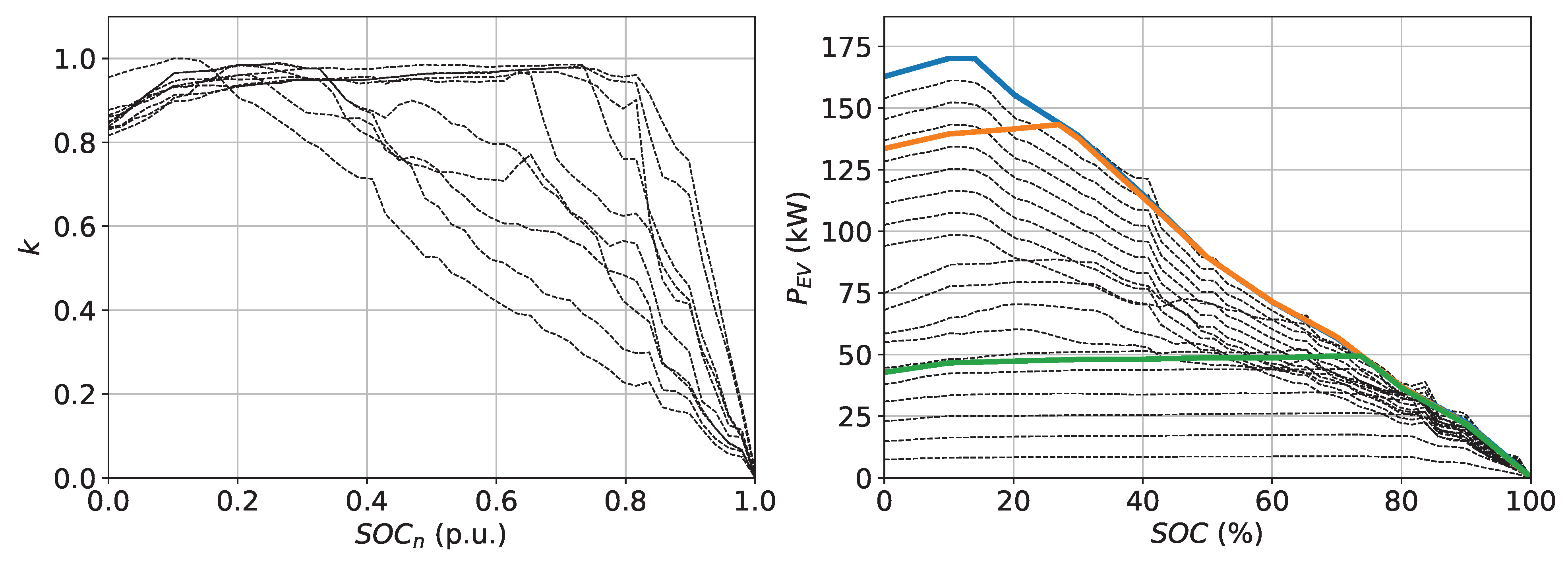
2.4. EV Battery Charging Behavioral Model Based on Machine Learning

The charging power $P_{\mathrm{EVi}}\left(t\right)$ is not constant during a charging process. The battery charger controls the charging profile to comply with the Constant Current-Constant Voltage (CC-CV) charging protocol for lithium batteries [17,31]. According to this protocol, the charge starts with the CC phase where a constant current is provided to the battery. During this phase, the battery voltage increases, and the power profile follows the one of the voltage. When the battery voltage reaches the upper cut-off value, the CV phase begins. During this phase, the charger keeps the battery voltage constant while the charging current decreases. Therefore, the power profile follows the current drop. The CV phase continues until the end of the charging.

The CC-CV charging phases can be conveniently described through the power–SOC curves [32] that are reported in Figure 7. Figure 7 shows the $P_{\mathrm{EV}}-SOC$ curves for different vehicle models considering different charging rates. It is possible to note (Figure 7a) that the higher the charging power, the more pronounced the CV phase. For the same EV model, the charging power profile depends on the SOC evolution and the C-rate ($C_{\mathrm{R}}$), i.e., the ratio between charging power and EV battery energy capacity $C_{\mathrm{B}}$ (in kWh). Moreover, different EV models may have different charging profiles. This is due to the differences in the EV’s hardware (i.e., battery, onboard charger, etc.), and firmware (mainly, the battery management system) adopted by the different manufacturers [18]. The aim of this Subsection is to investigate Battery Charging Behavioral Models (BCBM) that are capable of emulating power profiles and dynamically calculating the charging power of an EV as a function of SOC, C-rate, and vehicle model.

Focusing on a whole charging process, $P_{\mathrm{EVmax}}$ is the peak value of the power profile, which generally corresponds to the end of the CC phase. The value of $P_{\mathrm{EVmax}}$ depends on both the charging point power rating ($P_{\mathrm{CP}}$) and the maximum power that the vehicle battery can receive $P_{\mathrm{Bmax}}$. Finally, the peak value of the charging profile ($P_{\mathrm{EVmax}}$) corresponds to:

$$P_{\mathrm{EVmax}}=\min [P_{\mathrm{CP}},P_{\mathrm{Bmax}}]$$

(4)

Knowing the value of $P_{\mathrm{EVmax}}$, the charging power profile can be obtained as:

$$P_{\mathrm{EV}}=k(SOC,C_{\mathrm{R}},M_{\mathrm{ID}})P_{\mathrm{EVmax}}$$

(5)

where $k\in [0,1]$ is a normalization factor that varies during the charging process as a function of the $SOC$, the C-rate, and the EV model ($M_{\mathrm{ID}}$). The BCBM expressed by Equation (5) is based on a supervised machine learning predictive model. It defines the k-function through the training of the model via historical data, which encapsulates the dependence on the features ($SOC$, $C_{\mathrm{R}}$, $M_{\mathrm{ID}}$). The entire procedure of data processing, model training and validation is described below.

2.4.1. Data Pre-Processing

Predictive models, such as regression morels, work by establishing a relationship between variables in the data that represent characteristics of the quantity being observed (known as the features), and the variable being targeted for prediction (known as the label) [33]. In order to develop a predictive model via machine learning technique, a pre-processing of the data (i.e., the data population used for the model training) is required.

The training of the model is obtained starting from the measured charging profiles retrieved from [18]. The EV charging profiles (such as the curves reported in Figure 7) are collected and sampled to create the main data frame. Thus, for each punctual value of SOC, the value of $P_{\mathrm{EV}}$ is registered. The $P_{\mathrm{EV}}$ data are normalized as a function of the peak power value of the charging profile. The same process is carried out to the SOC in order to have normalized values, i.e., ($P_{\mathrm{EVn}}$, $SO{C}_{\mathrm{n}}$) $\in [0,1]$. Each pair ($P_{\mathrm{EVn}}$, $SO{C}_{\mathrm{n}}$) is matched with the vehicle model identification number ($M_{\mathrm{ID}}$) and the corresponding $C_{\mathrm{R}}$ value. The output of data pre-processing consists of a data frame in which each sampling observation is organized into four columns containing the label, i.e., $P_{\mathrm{EVn}}$, and the features $SO{C}_{\mathrm{n}}$, $C_{\mathrm{R}}$, and $M_{\mathrm{ID}}$. Figure 8 shows the output of the above-described data processing. Figure 8a shows the $P_{\mathrm{EVn}}\left(SO{C}_{\mathrm{n}}\right)$ curves colored as a function of $M_{\mathrm{ID}}$. On the other hand, Figure 8b shows the $P_{\mathrm{EVn}}\left(SO{C}_{\mathrm{n}}\right)$ curves colored as a function of $C_{\mathrm{R}}$.

2.4.2. Model Training

The use of historic data with known label values to train a model is also called “supervised machine learning”. The training process fits the features $x=[SO{C}_{\mathrm{n}},C_{\mathrm{R}},M_{\mathrm{ID}}]$ to the known label $y=P_{\mathrm{EVn}}$ to define a general function $F\left(x\right)$ that can be applied to new features for which the labels are unknown, and predict them. This is achieved by applying an algorithm that tries to fit the x values to a calculation that produces prediction reasonably accurately for all of the cases in the training dataset. Referring to Equation (5), it means identifying a model that minimizes the error between the sampled $P_{\mathrm{EVn}}(SO{C}_{\mathrm{n}},C_{\mathrm{R}},M_{\mathrm{ID}})$ and its prediction $F(SO{C}_{\mathrm{n}},C_{\mathrm{R}},M_{\mathrm{ID}})$. The model training, as well as data pre-processing, are carried out in Python by using the scikit-learn libraries [34,35].

Different regression methods can be used in machine learning, such as linear regression, decision forest regression, neural network regression, boosted decision tree regression, etc. Due to the high prediction accuracy, fast training time [36], and its particularly fitting to data sets of both continuous and categorical kind [37], the model used in this work is the Gradient Boosting Regressor (GBR). Gradient boosting is a machine learning technique used in regression (but also classification) tasks. It gives a prediction model in the form of an ensemble of weak prediction models, which are typically decision trees [38]. Unlike other regressors based on decision trees (such as the random forest regressor), the GBR learns from its mistakes in each iteration. It means that in gradient boosting, all trees are interconnected and each subsequent tree learns from the mistakes of the upstream ones by optimizing a differentiable loss function [39,40].

It’s common practice in supervised learning to split the data into two subsets [41]:

• A training dataset (typically larger than about 70% of the main data set) with which to train the model. It contains the training feature ($x_{\mathrm{train}}$) and label ($y_{\mathrm{train}}$) values;
• A test dataset (about 30% of the main dataset) with which to validate the trained model by generating predictions for the label and comparing them to the actual known label values. This enables to evaluate the model error and accuracy. The test dataset contains the test feature ($x_{\mathrm{test}}$) and label ($y_{\mathrm{test}}$) values.

It’s important to perform the splitting randomly. This helps ensure that the two data subsets are statistically comparable (i.e., the model is validated with data that has a similar statistical trend to the data on which it was trained).

The performance of the GBR algorithm strongly depends on the constituent parameters, such as the number of trees, the number of leaves and nodes of each tree, the learning rate, the loss function, etc. These setting parameters are generally called “hyper-parameters” of the model (i.e., parameters not directly learned within estimators). It is important to find the optimal setting of the hyper-parameters to have a good prediction performance.

The GBR model used in this work is the GradientBoostingRegressor [42] from the library sklearn.ensemble [34]. The model proposed by sklearn has several hyper-parameter that is possible to set for the tuning of the model. In this work, the focus is on the element of the vector ${\overline{H}}_{\mathrm{P}}=\left[M,\nu ,J_m\right]$ that represents the number of trees, the learning rate, and the number of leaves for each tree, respectively. The search for the optimal value of ${\overline{H}}_{\mathrm{P}}$ is carried out via an iterative deterministic process that considers combinations of the ${\overline{H}}_{\mathrm{P}}$-elements within pre-determined ranges of variation. This operation is performed using a “fit” and a “score” method, where the ${\overline{H}}_{\mathrm{P}}$-elements are optimized by cross-validated grid-search over a parameter grid [35]. The optimal values of ${\overline{H}}_{\mathrm{P}}$ are used to set the GBR model. Finally, the learning of the GBR model is performed on the population of the training dataset ($x_{\mathrm{train}},y_{\mathrm{train}}$).

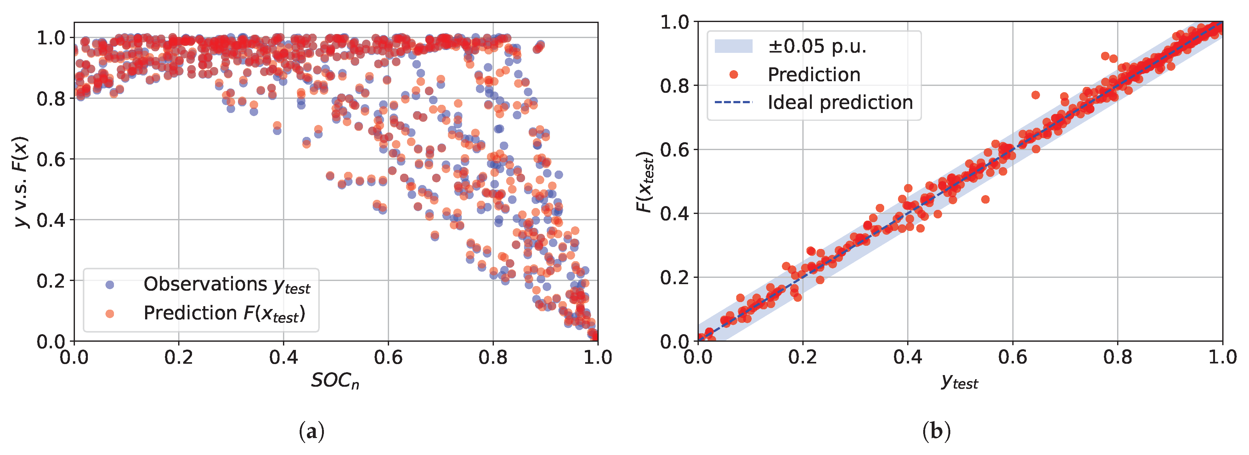
2.4.3. Model Validation

To validate the accuracy of the model trained through ($x_{\mathrm{train}},y_{\mathrm{train}}$), the test dataset is used. The validation procedure consists in comparing the model predictions $F\left(x_{\mathrm{test}}\right)$, which are made on the test features ($x_{\mathrm{test}}$), with the label of the test dataset ($y_{\mathrm{test}}$). In other words, the validation procedure evaluates the difference between the label predicted when the model applies the “behavior” it learned during training to the test data, and the actual value of the test label. The indicate the expected level of error when the model is used with new data for which the label is unknown [41].

An initial qualitative evaluation of the model’s performance can be taken graphically from Figure 9. The figure compares the actual observation of the test label $y_{\mathrm{test}}$ (blue markers) with respect to its predictions $F\left(x_{\mathrm{test}}\right)$ (red markers). Figure 9a provides the comparison as a function of the $SO{C}_n$ feature. It appears that the predictions are able to overlap adequately well with the observed samples. Finally, Figure 9b provides an evaluation of the residuals. The blue dashed line depicts the ideal zero-error prediction and the light-blue area represents a 5% error zone. It can be seen from Figure 9b that most of the $F\left(x\right)$ values overlap the dashed line and remain within the light-blue zone.

Quantitative validation of the model prediction performance is obtained using the following operator:

• Mean Square Error (MSE) that is the mean of the squared differences between predicted and actual values. The proposed GBR model obtains a value of MSE = 0.0003;
• Root Mean Square Error (RMSE) that is the square root of the MSE. This parameter yields an absolute metric in the same unit as the label (in this case, p.u.). The smaller the value, the better the model. The predictions overlap the observation with an RMSE = 0.0174;
• Coefficient of Determination (usually known as R-squared or R2). It is a relative metric that quantifies the fit of the model. In essence, this metric represents how much of the variance between predicted and actual label values the model is able to explain. A good trade-off to avoid over-fitting is R2 = 1 [43]. The proposed method score is R2 = 0.9959.

Finally, according to Equation (5), the trained model is encapsulated in the definition of the coefficient k (reporting the dependence on SOC from p.u. to percentage):

$$k=F\left(x\right)$$

(6)

Introducing the machine learning predictive model in Equation (6), it is possible to recreate the profile of $P_{\mathrm{EV}}$ for each value of SOC, C-rate, and vehicle model through Equation (5). Figure 10 shows, as an example, the results obtained considering the Tesla Model 3 RP (from the $M_{\mathrm{ID}}$ list). The left plots show the k value as a function of the SOC as the C-rate increases (i.e., $P_{\mathrm{EVmax}}$ increases). The right plots show the corresponding power–SOC profile computed via Equation (5) (dashed black lines). The colored markers in the figure represent the starting measured data from which the model was trained.

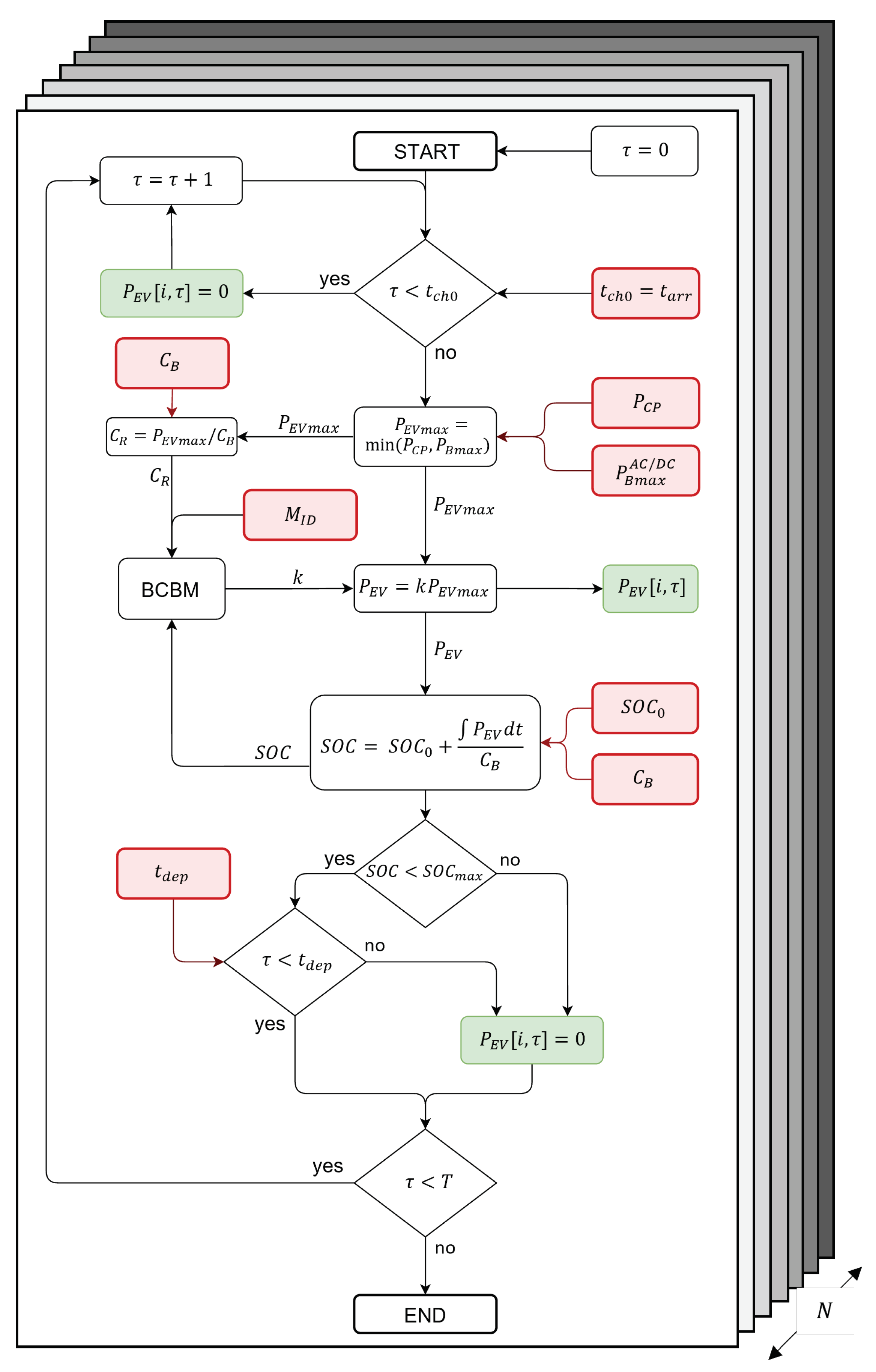
3. EV Charging Forecasting Algorithm

All results derived in Section 2 are integrated and used for developing the algorithm proposed in this work. The input data received by the algorithm are reported in

Table 3. Input and output data of the proposed algorithm.

Symbol	Description
input data
N	daily number of vehicles arriving to the CH
$P_{\mathrm{CP}}$	charging station power rating
$C_{\mathrm{CP}}$	charging station category, AC or DC charging point
S	parking lot scenario
output data
$P_{\mathrm{EVi}}\left(t\right)$	daily power profile of each $E{V}_{i\in N}$
$P_{\mathrm{CH}}\left(t\right)$	daily total power profile required by the whole CH
$SO{C}_i\left(t\right)$	state of charge evolution of each $E{V}_{i\in N}$

. From this data, the algorithm computes the daily power profile $P_{\mathrm{EVi}}\left(t\right)$ of each $E{V}_{i\in N}$ and calculates the daily total power profile required by the whole CH, $P_{\mathrm{CH}}$.

The algorithm is initialized by the parameters of the N-EVs population then it collects the related information in an initialization data frame. This data frame, called $ID$, consists of N rows and each row reports information about the related $E{V}_i$. By way of example,

Table 4. Example of the initialization data frame ($ID$) of a 5-vehicles population.

${\mathbf{EV}}_{\mathbf{ID}}$	Model	${\mathit{M}}_{\mathbf{ID}}$	${\mathit{C}}_{\mathbf{B}}$	${\mathbf{SOC}}_0$	${\mathit{P}}_{\mathbf{Bmax}}^{\mathbf{AC}}$	${\mathit{P}}_{\mathbf{Bmax}}^{\mathbf{DC}}$	${\mathit{t}}_{\mathbf{arr}}$	${\mathit{t}}_{\mathbf{dep}}$	${\mathit{T}}_{\mathbf{pk}}$
1	FIAT 500e	0	37.3	34	11	85	8:15	15:00	6.75
2	Tesla M3	4	75	23	11	210	10:00	17:45	7.75
3	Renault ZOE	13	52	67	22	46	7:45	10:30	2.25
4	FIAT 500e	0	37.3	51	11	85	9:30	16:00	6.50
5	VW UP!	8	36.8	15	7.4	40	8:00	12:00	4.00

shows the initialization data frame of a population of 5 EVs. The $ID$ data frame contains information about the EVs population derived from the distribution of the models’ share summarized in Figure 3. Along with the EV model, $ID$ reports the corresponding value of battery capacity $C_{\mathrm{B}}$ (in kWh), the ID number associated to each model, and the maximum charging capability in AC ($P_{\mathrm{Bmax}}^{AC}$) and DC ($P_{\mathrm{Bmax}}^{DC}$) modes (both in kW). To each $E{V}_i$ is assigned a $SO{C}_{0\mathrm{i}}$ value (in percent). The $SO{C}_{0\mathrm{i}}$ is obtained according to the procedures described in Section 2.3.

The last columns of $ID$ report the arrival time, departure time, and parking duration of the i-th EV (expressed in hours). These values are obtained considering the analysis carried out in Section 2.2 and according to the selected parking lot scenario S. The values of $t_{\mathrm{arr}}$, $t_{\mathrm{dep}}$, and the relative $T_{\mathrm{pk}}$ are computed starting from their distribution so as to obtain a population of N samples whose probabilistic trend respects that of the selected scenario.

For each $E{V}_i$, the charging time $T_{\mathrm{ch},\mathrm{i}}$ is defined as the period between the initial time of charging $t_{\mathrm{ch}0,\mathrm{i}}$, that is the instant in which $E{V}_i$ is plugged in, and the final time of charging $t_{\mathrm{ech},\mathrm{i}}$:

$$T_{\mathrm{ch}}=t_{\mathrm{ech}}-t_{\mathrm{ch}0}$$

(7)

The end-charging time $t_{\mathrm{ech},\mathrm{i}}$ may depend on two conditions:

• The vehicle is plugged and the SOC reaches the maximum value. Hence, the charging stops and $SO{C}_i\left(t_{\mathrm{ech}}\right)=SO{C}_{\max }$;
• The vehicle is unplugged because the users leaves the parking lot even if the charging is incomplete. Hence, $SO{C}_i\left(t_{\mathrm{ech}}\right)<SO{C}_{\max }$.

It is assumed that the instant of arrival in the parking lot coincides with the beginning of the charging, therefore:

$$t_{\mathrm{ch}0}=t_{\mathrm{arr}}\Rightarrow SOC\left(t_{\mathrm{ch}0}\right)=SO{C}_0$$

(8)

On the other hand, the final charging instant could coincide or not with the departure time of the vehicle from the parking lot. This condition is governed by the following equation set:

$$t_{\mathrm{ech}}<t_{\mathrm{dep}}\Rightarrow SOC\left(t_{\mathrm{ech}}\right)=SO{C}_{\max }$$

(9a)

$$t_{\mathrm{ech}}=t_{\mathrm{dep}}\Rightarrow SOC\left(t_{\mathrm{ech}}\right)<SO{C}_{\max }$$

(9b)

The second step of the proposed method is to define, for each i-th EV, an array that contains the value of $P_{\mathrm{EVi}}$ for each discretized instant $\tau$ of the day. In this work, a discretization time resolution $\Delta \tau =1\min$ is considered. Thus, the $P_{\mathrm{EVi}}$-array for a 1-day calculation consists of $T=1440$ elements. Considering the whole population of N EVs it is possible to define the $N\times T$ matrix ${\mathit{P}}_{\mathbf{EV}}$ whose element $P_{\mathrm{EV}}[i,\tau ]$ represents the power required by the i-th EV (row-index) at the $\tau$-th minute of the day (column-index). Similarly, it is possible to define the matrix describing the vehicle presence in the parking lot, called $\mathit{PK}$, and the matrix of the $SOC\left(t\right)$ evolution, called $\mathit{SOC}$. The elements of $\mathit{PK}$ are of Boolean kind; specifically $PK[i,\tau ]=1$ if the i-th vehicle is parked at instant $\tau$, otherwise $PK[i,\tau ]=0$. The element $SOC[i,\tau ]$ represents the state of charge of $E{V}_i$ at the instant $\tau$. It is clear that $SOC{[i,\tau ]}_{\tau =t_{\mathrm{ch}0}}=SO{C}_{0\mathrm{i}}$ and is initialized through the value of the $ID$ data frame. The following forecasting algorithm logic is shown in Figure 11.

Considering an N-users population the algorithm runs in parallel for each EV (${\mathit{P}}_{\mathbf{EV}}$-row) in order to fill all the elements of the ${\mathit{P}}_{\mathbf{EV}}$ matrix. The algorithm starts the calculation by referring at the time $\tau =0$ (beginning of the day, i.e., 00:00). For each $E{V}_i$ the algorithm is initialized through the i-row of the $ID$ data frame, whose data are represented by the red box in the flow chart of Figure 11. The resulted powers are highlighted through the green boxes.

As long as $\tau <t_{\mathrm{ch}0}$, the vehicle is not present and $PK[i,\tau ]=0$, the output $P_{\mathrm{EV}}[i,\tau ]$ is zero. As soon as the vehicle arrives in the parking lot, $PK[i,\tau ]$ switches to one and keeps this value as long as the vehicle is parked. $SOC[i,\tau ]$ is initialized to $SO{C}_{0\mathrm{i}}$ and the algorithm starts calculating the charging power.

After that, the initial value of the power is multiplied by a scale factor k according to Section 2.4. The k parameter is the output of the BCBM and sets the power absorption of $E{V}_i$ according to its $M_{ID}$, $SOC$, and relative C-rate. The algorithm updates the SOC in each iteration by calculating the battery’s energy through charging power integration. Accordingly, the element $SOC[i,\tau ]$ of $\mathit{SOC}$ at the instant $\tau$ is obtained by Equation (10):

$${\displaystyle SOC[i,\tau ]=SOC[i,t_{\mathrm{ch}0}]+{\displaystyle \frac{{\sum }_{\zeta =t_{\mathrm{ch}0}}^{\tau }{P}_{\mathrm{EV}}[i,\zeta ]\Delta \tau }{C_{\mathrm{Bi}}}}}$$

(10)

where $SOC[i,t_{\mathrm{ch}0}]=SO{C}_{0\mathrm{i}}$ and the term ${\sum }_{\zeta =t_{\mathrm{ch}0}}^{\tau }{P}_{\mathrm{EV}}[i,\zeta ]\Delta \tau$ represent the cumulative energy (kWh) from the start of charging to the $\tau$-instant. The charging process can stop ($P_{\mathrm{EV}}[i,\tau ]=0$) if condition of Equation (9a) or (9b) occurs. Finally, the algorithm stops computing at $\tau =T$ (end of the day, i.e., 24:00).

Once the ${\mathit{P}}_{\mathbf{EV}}$ matrix is calculated for each $\tau \in T$ it is possible to obtain the total power profile of the charging hub containing the contribution of each $E{V}_{i\in N}$:

$$P_{\mathrm{CH}}\left[\tau \right]=\sum _{i=1}^N{P}_{\mathrm{EV}}[i,\tau ]$$

(11)

As an example, Figure 12 shows the results of the proposed algorithm considering a 100-EV population and a charging hub having AC CPs of $P_{\mathrm{CP}}=22\mathrm{kW}$. The charging hub is located in a working place parking lot. The scatter plot in Figure 12a shows the arrival and departure time randomly generated from their scenario pattern (Figure 4c). Figure 12a also shows $P_{\mathrm{EVi}}$ as a heat map. The heat map represents the power level that the EVs require from the CPs during the charge. The color variations depend on the modulation due to the BCBM. Figure 12b shows the charging power profile of each EV belonging to the N-users population. It is evident how the power profile varies during charging depending on the vehicle model, C-rate, and the evolution of the SOC. Although $P_{\mathrm{CP}}=22\mathrm{kW}$, only a portion of EVs manage to use all of CP power (mainly the Renault ZOE). Most vehicles receive a maximum power output of $11\mathrm{kW}$ or less. Figure 12c shows the value of the SOC at the arrival time and at the departure time. The black dashed line depicts the evolution of the state of charge as a function of time, $SO{C}_i\left(t\right)$. Finally, Figure 12d shows the total power required by the charging hub, $P_{\mathrm{CH}}$ obtained from Equation (11). The figure shows a peak of about $400\mathrm{kW}$ at the peak of EV arrivals. Through the algorithm, it is also possible to calculate the total energy required daily by the CH, which is about $2200\mathrm{kWh}$ and is represented by the blue area in Figure 12d.

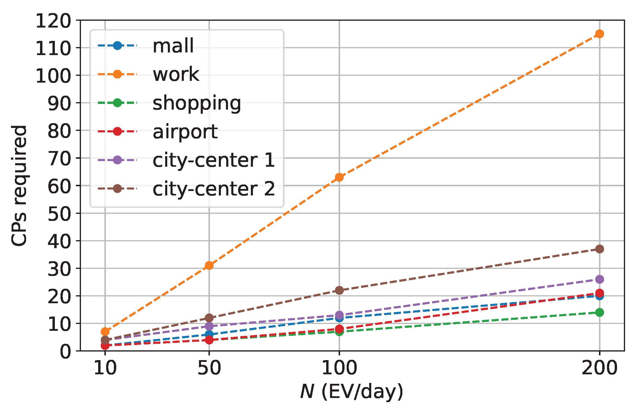
4. Results on Different Scenarios

The following section analyzes and discusses the results obtained from the proposed forecasting algorithm. Comparisons are conducted considering the possible variations of the algorithm setting parameters. Specifically, the effects on the power profile of the number of daily users, the charging stations’ power rating, and the parking scenario are analyzed in detail.

Table 5. Setting of the algorithm input parameter used in this section.

Input Parameter	Simulation Setting Value												Unit
$P_{\mathrm{CP}}$	3.6	7.4	11	22	25	50	75	100	150	200	250	350	kW
$C_{\mathrm{CP}}$	AC	AC	AC	AC	DC	DC	DC	DC	DC	DC	DC	DC	-
N	10, 50, 100, 200												EV/day
S	work, mall, airport, city center 1, city center 2, shopping												-

shows the settings of the algorithm input parameters selected to compare the results.

The values of $P_{\mathrm{CP}}$ is set to match all the charging level categories reported in Table 1, from slow AC-charging to ultra-fast DC-charging. The $C_{\mathrm{CP}}$ is set according to the related power level. Four charging hub daily users numbers from 10 to 200 EV/day are selected in order to evaluate a possible temporal increase in EV penetration or a different size of the parking area.

Figure 13 and Figure 14 show some preliminary results. The figures represent the daily power profiles (24-h time window) for 4 different scenarios as the charging points’ power and the number of daily users change. The gray lines depict $P_{\mathrm{CH}}\left(t\right)$ (with a 1-min resolution). The dashed colored lines depict the $P_{\mathrm{CH}}$ moving average whose color is a function of the N-setting. The $P_{\mathrm{CP}}$ selected for Figure 13 and Figure 14 are $22\mathrm{kW}$ (that is the upper limit of the most common AC-charging level) and $150\mathrm{kW}$ (that is the upper limit of the most common DC category).

It is possible to see how the profiles are more pulsed the higher is the CP power. This phenomenon is mainly due to the arrival of new users who can each potentially increase consumption by $150\mathrm{kW}$ at the instant of connection. The CH peak power is also naturally affected by $P_{\mathrm{CP}}$ and N. In addition, the results show that the peak power and, in general, the evolution of the whole profile strongly depend on the scenario S under consideration.

For the same number of daily users, the scenario with a more concentrated distribution of arrivals and longer parking time exhibits a contemporaneity of charging events. More users connected for a longer time implies a higher demand for instantaneous power and total energy. This phenomenon can be observed by comparing Figure 13a,c with Figure 13b,d. As described in Section 2.2, the “working” scenario has a more concentrated distribution of arrivals (peaking around 8 a.m.) and a longer average parking time. This affects the simultaneity of charging events compared to the “mall” scenario, which instead has a more distributed probability of arrivals and a shorter vehicle dwell time. As a result, Figure 13b,d shows higher peaks (about twice as high) than Figure 13a,c. This difference is more pronounced the higher the number of daily CH users N. Similar considerations can be done in Figure 14 where another parking scenario in analyzed.

Based on the parking lot scenario, it is possible to analyze the simultaneity of the charging events through Figure 15. The proposed algorithm allows us to evaluate the instant and the duration of the users’ connection time. Then, it is possible to calculate the number of users simultaneously connected to the charging hub. From a complementary point of view, Figure 15 shows the number of CPs that the CH should have to satisfy the entire fleet of N users per day.

It is therefore possible to state that the parking scenario influences the sizing of the CH in terms of peak power required, the number of CPs to be installed to satisfy the entire fleet of N users (simultaneity of charging events), and finally the average energy deliverable to vehicles. The following sections quantitatively analyze the results by comparing the scenarios in these respects.

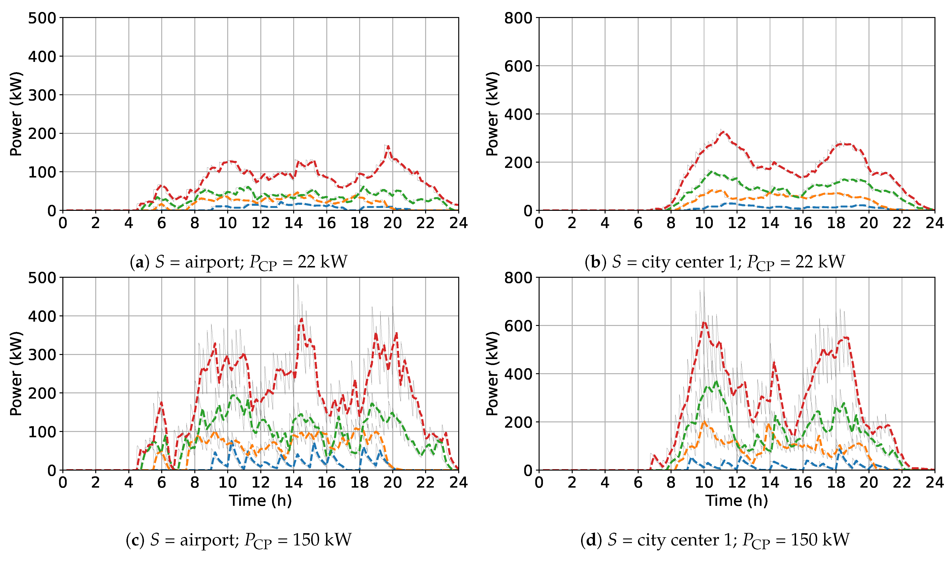
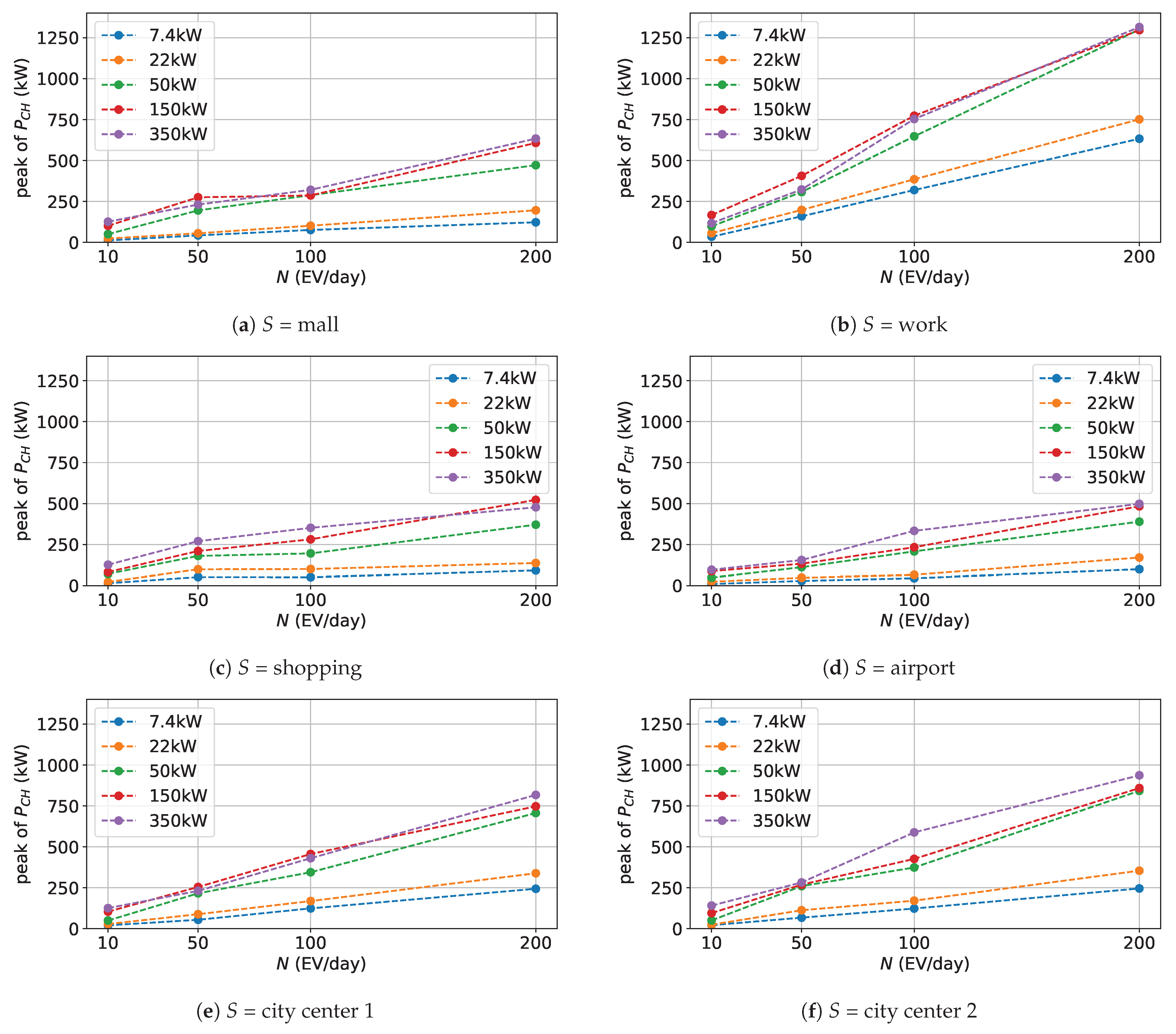
4.1. Analysis on the Charging Hub Peak Power

Although the simulations are initialized with models that follow a defined pattern, the individual elements of the initialization data frame ($ID$, Table 4) own a random nature. Therefore, it may occur that the algorithm generates slightly different power profiles despite being set with the same input values. To provide adequate statistical significance to the results shown in the following, multiple simulations are performed for each input data setting. The final output results from the averaging of the values of each simulation run.

Assuming that the CH is sized to have the optimal number of CPs to satisfy all users (as in Figure 15), Figure 16 shows the peak power absorbed by the CH (peak of $P_{\mathrm{CH}}$) from the grid as a function of N for the scenarios under study. Different colors in Figure 16 depict different values of the CP power $P_{\mathrm{CP}}$. The most common sub-categories of Table 1 are selected for comparison.

The figure shows a quite linear proportionality between N and the peak value of the CH power profile. Specifically, the analysis conducted in this subsection confirms the dependence of $P_{\mathrm{CP}}$ on the number of EVs simultaneously connected (Figure 15).

On the other hand, results show that there is no direct proportionality between the peak power and the power rating available at the charging points. For example, let refer to the case $N=200$ in Figure 16e which considers the “city center 1” scenario. The greatest increase in peak power occurs at the transition from $22\mathrm{kW}$ to $50\mathrm{kW}$. Thereafter, tripling the CP power does not imply a noticeable increase in peak power. Moreover, in almost all the scenarios analyzed, from Fast to Ultra-fast CPs, the peak power variation is very slight in comparison to the $P_{\mathrm{CP}}$ variation. This is mainly due to the few numbers of EVs having a charging capability above $150\mathrm{kW}$ among the total population (as reported in Figure 3). This means that currently, for the same number of daily users and available CPs, the contracted power of a CH that has $150\mathrm{kW}$ CPs could potentially be similar to a CH that has $350\mathrm{kW}$ CPs.

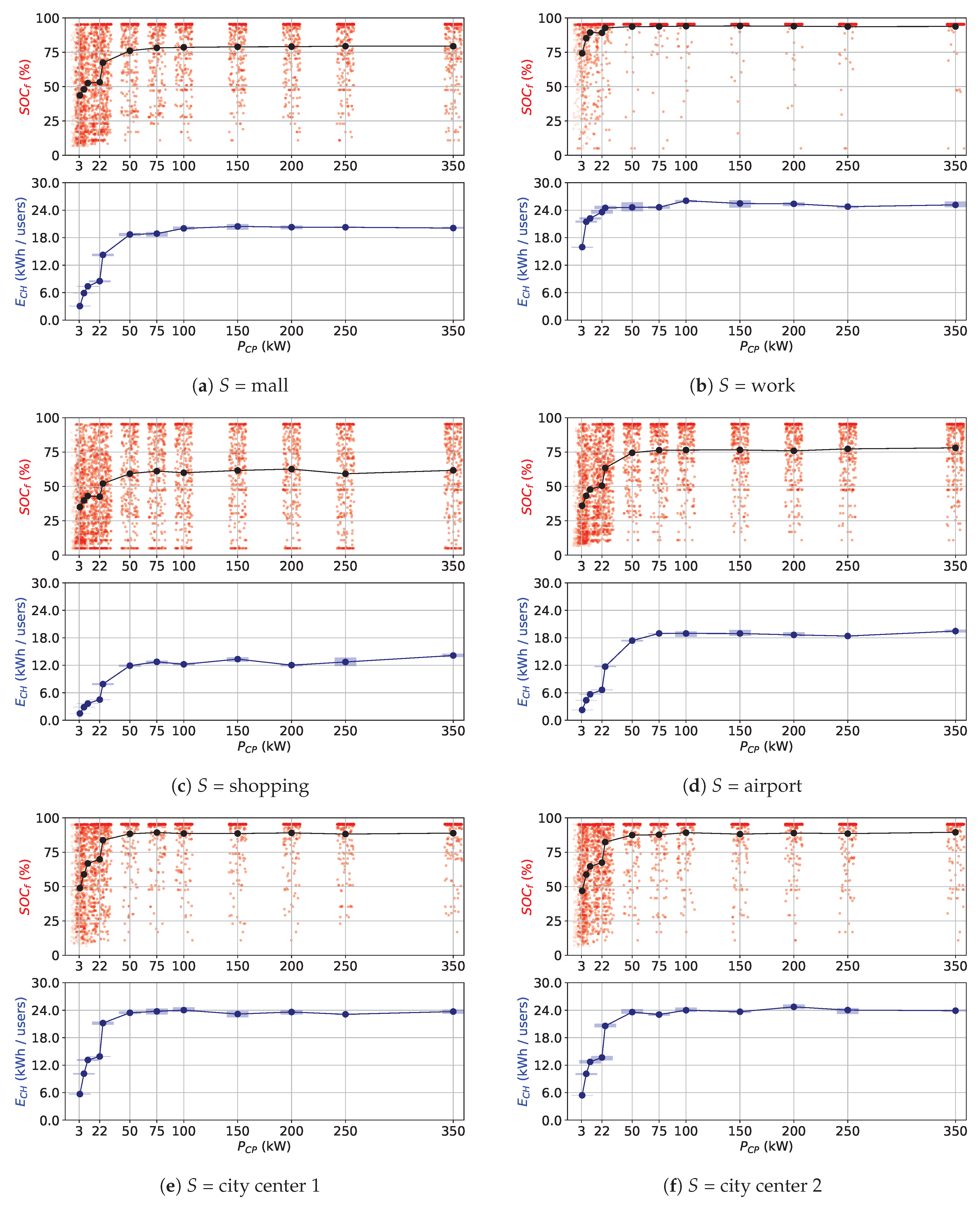
4.2. Analysis on the EV Fleet Charged Energy

This subsection compares the total energy provided to the EVs by the CH under different input settings. The total daily energy that CH supplies to the EVs, named $E_{\mathrm{CH}}$, depends on the charging power $P_{\mathrm{CP}}$ and charging time $T_{\mathrm{pk}}$. However, the real values of used power is limited by the maximum power $P_{\mathrm{EV}}$ that the vehicle’s battery and onboard converter can accept. Therefore, there could be a sort of threshold value of $P_{\mathrm{CP}}$ beyond which, further increase in the nominal power of the CPs would not result in an increases in the total energy delivered to the EV population batteries. The parking scenario influences users’ parking time and thus, for the same power output, itaffects the total daily energy delivered to EVs. It may be possible that scenarios with lower $T_{\mathrm{pk}}$ require higher $P_{\mathrm{CP}}$ to meet the energy needs of EVs.

Through the proposed method, it is possible to address these issues and evaluate the CH’s ability to meet vehicle energy demand under different parking scenarios. The comparison proposed in this section focuses on the daily average energy supplied to the EV population (kWh/users) and their average state of charge at the departure time ($SO{C}_{\mathrm{f}}$). Simulations run considering $N=100$ for each S. The value of $P_{\mathrm{CP}}$ varies in the range shown in Table 5. Figure 17 shows the values of EVs’ SOC at the departure time, which are depicted by the red dots (top-frame of the sub-figures). The black line with round markers represents the average value of $SO{C}_{\mathrm{f}}$. On the bottom frame of the sub-figures, the blue markers depict the average energy supplied per EV (kWh/user).

The figures point out clear differences among scenarios. In the working place parking scenario (Figure 17b), results show that high power levels do not imply significant additional increase in $SO{C}_{\mathrm{f}}$ and $E_{\mathrm{CH}}$. This is due to the longer $T_{\mathrm{pk}}$, where EVs stay parked long enough to ensure adequate $SO{C}_{\mathrm{f}}$ even at low $P_{\mathrm{CP}}$. The figure shows a slight increase in $E_{\mathrm{CH}}$ at the transition between AC and DC charger ($22\mathrm{kW}$ to $25\mathrm{kW}$) due to the bypass of the onboard charger that enables charging at higher powers. Higher values of $P_{\mathrm{CP}}$ seem to produce no improvement in delivered energy $E_{\mathrm{CH}}$, that remains at $26\mathrm{kWh}/\mathrm{user}$, and in the average $SO{C}_{\mathrm{f}}$, whose value remains close to $SO{C}_{\max }=95\%$).

Considering other scenarios which have a lower $T_{\mathrm{pk}}$, it is evident how switching from AC $22\mathrm{kW}$ to DC $25\mathrm{kW}$ CPs results in a significant increase in the delivered energy and the associated average $SO{C}_{\mathrm{f}}$. The Figure 17a,d–f show that for a small increase of $+3\mathrm{kW}$ in $P_{\mathrm{CP}}$, the energy delivered per vehicle doubles, and $SO{C}_{\mathrm{f}}$ exhibits a radical increase. For example, Figure 17e,f show that $E_{\mathrm{CH}}$ increases from 13 to 20 kWh/users and the average SOC from 66% to 82% in the case of city-center scenarios. Thereafter, performance increases as $P_{\mathrm{CP}}$ increases and then saturates at $P_{\mathrm{CP}}$ between $50\mathrm{kW}$ and $75\mathrm{kW}$. In the case of shopping scenario (Figure 17c) where the parking time is extremely short, even if $P_{\mathrm{CP}}$ increases the energy delivered to EVs cannot reach more than 14 $\mathrm{kW}/\mathrm{user}$ and the increase in $SO{C}_{\mathrm{f}}$ is negligible.

It is important to emphasize that the results obtained are valid under the assumption expressed by Equation (9b), or, in other words, that the charging time is considered equal to the parking time. Clearly, this assumption loses its validity in the event that the user extends the parking time to reach an higher SOC at departure. However, it is worth reiterating that the analysis performed aims precisely to investigate the capability of the CH to provide adequate energy to users without altering their behavior (i.e., usual parking time).

Results show that, in general, Slow DC charging points enable better performance in terms of $E_{\mathrm{CH}}$ and $SO{C}_{\mathrm{f}}$ compared to AC chargers having similar power ratings. Considering the working scenario, the AC medium-level charging is sufficient to ensure adequate $SO{C}_{\mathrm{f}}$ to the whole EV fleet. For all other scenarios analyzed, a good trade-off between $E_{\mathrm{CH}}$, $SO{C}_{\mathrm{f}}$ values and the CP power output is $P_{\mathrm{CP}}\in [50,75]\mathrm{kW}$. Fast and Ultra-fast charging point seems not to bring an improvement in the performance markers under study.

Finally,

Table 6. Summary of the analysis carried out in this section a 100-EV fleet.

Parking Scenario (S)	Optimal CP Number (N = 100 EV/day)	Optimal ${\mathit{P}}_{\mathbf{CP}}$ (kW)	Peak of ${\mathit{P}}_{\mathbf{CH}}$ (kW)	Average ${\mathit{E}}_{\mathbf{CH}}/\mathbf{EV}$ (kWh/EV)
mall	12	50 (DC)	288	18
working	63	22 (AC)	385	25
shopping	7	75 (DC)	200	12
airport	8	75 (DC)	250	18
city center 1	13	50 (DC)	344	24
city center 2	22	50 (DC)	377	24

shows the summary of the analysis carried out in this section. The table compares the scenarios considering N = 100 users per day. For each scenario, the table reports the number of CPs needed to ensure connection to each EV in the fleet, the CP power rating suggested to avoid over-sizing and ensure an adequate $SO{C}_{\mathrm{f}}$, the peak value of the CH power, and the average energy supplied per user.

5. Conclusions

The work has aimed at providing a method for forecasting the power demand related to a charging hub for EVs in different parking scenarios.

The method tried to take into account all the main factors that may influence the power demand. The preliminary analyses on the charging stations and EV models currently available revealed a significant heterogeneity in the values of power levels of the charging stations and in the battery capacities and accepted power levels for the recharge among the different EV models. At the same time, the absorbed power profile of a charging hub is influenced by other factors such as the arrival and departure time, and parking duration of EV users. These parameters change strongly according to different parking scenarios (e.g. malls, airports, urban car parks, etc.) Finally, for each charging process, the EV energy demand also depends on the state of charge at arrival at the charging hub.

Given the complexity, numerousness, and aleatory nature of the various factors considered, a probabilistic approach was used to generate a model of the vehicle population and user behavior under different parking scenarios in terms of arrival, departure, and parking duration times. The analysis of an extremely large sample of trips combined with the statistical distribution of the battery capacities of the electric vehicles on the road and the charging needs as a function of distance traveled has made possible to obtain a distribution of the state of charge of the EVs at their arrival at the charging hub. A supervised machine-learning model has been adopted to reproduce the behaviour of the battery during the charge as a function of the charging rate, the considered EV model and the evolution of the SOC during the charge. The model allowed to obtain the absorbed power profile associated to each charging event. The model has been trained and tested by using the power curves of different EV models, under different charging rates. The derived model has fit the test data with an RMSE = 0.017 and R2 = 0.996.

The resulting models from each analysis have been integrated in the final algorithm capable of forecasting the absorbed power for the charging of an electric vehicle fleet in the time domain.

The results section compares the algorithm outputs considering different combinations of the input data, namely: the parking scenario, the number of daily EV users, and the characteristics of the charging infrastructure (i.e., power rating and category of the CPs). The proposed algorithm proved its high effectiveness in assessing all major aspects essential for planning and sizing charging hubs in different installation scenarios. As shown in the results section, the algorithm allowed the evaluation of the optimal number of CPs to be installed to satisfy the demand of a certain EV fleet, the peak power required by the CH from the grid and the total energy daily delivered to each vehicle together with their final state of charge.

Analysis of the results showed marked differences between the power profiles of the scenarios analyzed. CH located in a working place scenario requires more CPs to satisfy the same number of users per day compared to other urban scenarios. On the other hand, $22\mathrm{kW}$ AC charging points are sufficient to meet the energy demand of the entire fleet. In fact, the results proven that DC chargers do not introduce significant improvements. The other urban scenarios, which have a lower probability of simultaneous user connection, require fewer CPs for the same number of daily charging events. However, due to the shorter parking times, fast DC CPs are needed to ensure an adequate energy supply. In this case, rated powers between $50\mathrm{kW}$ and $75\mathrm{kW}$ are sufficient to meet fleet energy demand. In general, considering the characteristics of the current EV population and the typical parking times of urban scenarios, the proposed method showed that the use of ultra-fast (i.e., $P_{\mathrm{CP}}>150\mathrm{kW}$) charging points produces no increase in average energy delivered. Similar considerations can be made regarding the SOC level of vehicles at the end of charging and the total peak power.

Future works can consider new parking scenarios like residential, home charging, and highway parking. Moreover, also the residential overnight charging can be considered for the computation of the pre-connection SOC. Finally, starting from the proposed EV load forecasting, future research can investigate sizing methods to optimize the design and management of PV and battery systems integrated with the charging hub.

References

1. Csonka, B.; Csiszár, C. Determination of charging infrastructure location for electric vehicles. Transp. Res. Procedia 2017, 27, 768–775. [Google Scholar] [CrossRef]
2. Andrenacci, N.; Ragona, R.; Valenti, G. A demand-side approach to the optimal deployment of electric vehicle charging stations in metropolitan areas. Appl. Energy 2016, 182, 39–46. [Google Scholar] [CrossRef]
3. Fitzgerald, G.; Nelder, C.; Newcomb, J. Electric Vehicles as Distributed Energy Resources; Rocky Mountain Institute: Boulder, CO, USA, 2016. [Google Scholar]
4. Deb, S.; Kalita, K.; Mahanta, P. Review of impact of electric vehicle charging station on the power grid. In Proceedings of the 2017 International Conference on Technological Advancements in Power and Energy (TAP Energy), Kollam, India, 1–23 December 2017; pp. 1–6. [Google Scholar] [CrossRef]
5. Clement, K.; Haesen, E.; Driesen, J. Stochastic analysis of the impact of plug-in hybrid electric vehicles on the distribution grid. In Proceedings of the CIRED 2009—20th International Conference and Exhibition on Electricity Distribution—Part 1, Prague, Czech Republic, 8–11 June 2009; pp. 1–4. [Google Scholar]
6. Gomez, J.; Morcos, M. Impact of EV battery chargers on the power quality of distribution systems. IEEE Trans. Power Deliv. 2003, 18, 975–981. [Google Scholar] [CrossRef]
7. Lo Franco, F.; Cirimele, V.; Ricco, M.; Monteiro, V.; Afonso, J.L.; Grandi, G. Smart charging for electric car-sharing fleets based on charging duration forecasting and planning. Sustainability 2022, 14, 12077. [Google Scholar] [CrossRef]
8. Lo Franco, F.; Ricco, M.; Mandrioli, R.; Grandi, G. Electric vehicle aggregate power flow prediction and smart charging system for distributed renewable energy self-consumption optimization. Energies 2020, 13, 5003. [Google Scholar] [CrossRef]
9. Fouladi, E.; Baghaee, H.R.; Bagheri, M.; Gharehpetian, G. Power management of microgrids including PHEVs based on maximum employment of renewable energy resources. IEEE Trans. Ind. Appl. 2020, 56, 5299–5307. [Google Scholar] [CrossRef]
10. Lo Franco, F.; Mandrioli, R.; Ricco, M.; Monteiro, V.; Monteiro, L.F.; Afonso, J.L.; Grandi, G. Electric Vehicles Charging Management System for Optimal Exploitation of Photovoltaic Energy Sources Considering Vehicle-to-Vehicle Mode. Front. Energy Res. 2021, 9, 716389. [Google Scholar] [CrossRef]
11. Ramadhani, U.H.; Fachrizal, R.; Shepero, M.; Munkhammar, J.; Widén, J. Probabilistic load flow analysis of electric vehicle smart charging in unbalanced LV distribution systems with residential photovoltaic generation. Sustain. Cities Soc. 2021, 72, 103043. [Google Scholar] [CrossRef]
12. Vehicles and Fleet|European Alternative Fuels Observatory. Available online: https://alternative-fuels-observatory.ec.europa.eu/transport-mode/road/european-union-eu27/vehicles-and-fleet (accessed on 22 December 2022).
13. Immatricolazioni in Italia di Autovetture e Fuoristrada Top-20 BEV 2021. Available online: https://unrae.it/dati-statistici/immatricolazioni (accessed on 22 December 2022).
14. Infrastructure|European Alternative Fuels Observatory. Available online: https://alternative-fuels-observatory.ec.europa.eu/transport-mode/road/european-union-eu27/infrastructure (accessed on 22 December 2022).
15. Hypercharger by Alpitronic, Model HYC300|Web Site. Available online: https://www.hypercharger.it/hyc300-2/ (accessed on 22 December 2022).
16. EV Database. Available online: https://ev-database.org/ (accessed on 22 December 2022).
17. Shen, W.; Vo, T.T.; Kapoor, A. Charging algorithms of lithium-ion batteries: An overview. In Proceedings of the 2012 7th IEEE conference on industrial electronics and applications (ICIEA), Singapore, 8–20 July 2012; pp. 1567–1572. [Google Scholar]
18. Vehicles-Fastned FAQ. Available online: https://support.fastned.nl/hc/en-gb/categories/4428895407133-Fastned-charging (accessed on 22 December 2022).
19. Lee, D.H.; Kim, M.S.; Roh, J.H.; Yang, J.P.; Park, J.B. Forecasting of Electric Vehicles Charging Pattern Using Bayesians method with the Convolustion. IFAC-PapersOnLine 2019, 52, 413–418. [Google Scholar] [CrossRef]
20. Zhou, D.; Guo, Z.; Xie, Y.; Hu, Y.; Jiang, D.; Feng, Y.; Liu, D. Using Bayesian Deep Learning for Electric Vehicle Charging Station Load Forecasting. Energies 2022, 15, 6195. [Google Scholar] [CrossRef]
21. Zhuang, Z.; Zheng, X.; Chen, Z.; Jin, T.; Li, Z. Load Forecast of Electric Vehicle Charging Station Considering Multi-Source Information and User Decision Modification. Energies 2022, 15, 7021. [Google Scholar] [CrossRef]
22. Boulakhbar, M.; Farag, M.; Benabdelaziz, K.; Kousksou, T.; Zazi, M. A deep learning approach for prediction of electrical vehicle charging stations power demand in regulated electricity markets: The case of Morocco. Clean. Energy Syst. 2022, 3, 100039. [Google Scholar] [CrossRef]
23. Almaghrebi, A.; Aljuheshi, F.; Rafaie, M.; James, K.; Alahmad, M. Data-driven charging demand prediction at public charging stations using supervised machine learning regression methods. Energies 2020, 13, 4231. [Google Scholar] [CrossRef]
24. Nespoli, A.; Ogliari, E.; Leva, S. User Behaviour Clustering Based Method for EV Charging Forecast. IEEE Access 2023. [Google Scholar] [CrossRef]
25. Recharging Systems|European Alternative Fuels Observatory. Available online: https://alternative-fuels-observatory.ec.europa.eu/general-information/recharging-systems (accessed on 22 December 2022).
26. Schmenger, J.; Endres, S.; Zeltner, S.; März, M. A 22 kW on-board charger for automotive applications based on a modular design. In Proceedings of the 2014 IEEE Conference on Energy Conversion (CENCON), Johor Bahru, Malaysia, 13–14 October 2014; pp. 1–6. [Google Scholar]
27. Arif, S.M.; Lie, T.T.; Seet, B.C.; Ayyadi, S.; Jensen, K. Review of electric vehicle technologies, charging methods, standards and optimization techniques. Electronics 2021, 10, 1910. [Google Scholar] [CrossRef]
28. European Union (EU27)|European Alternative Fuels Observatory. Available online: https://alternative-fuels-observatory.ec.europa.eu/transport-mode/road/european-union-eu27 (accessed on 22 December 2022).
29. Federal Highway Administration. National Household Travel Survey; U.S. Department of Transportation: Washington, DC, USA, 2017. Available online: https://nhts.ornl.gov (accessed on 22 December 2022).
30. Franco, F.L.; Ricco, M.; Mandrioli, R.; Paternost, R.F.; Grandi, G. State of Charge Optimization-based Smart Charging of Aggregate Electric Vehicles from Distributed Renewable Energy Sources. In Proceedings of the 2021 IEEE 15th International Conference on Compatibility, Power Electronics and Power Engineering (CPE-POWERENG), Florence, Italy, 14–16 July 2021; pp. 1–6. [Google Scholar] [CrossRef]
31. Franco, F.L.; Ricco, M.; Mandrioli, R.; Viatkin, A.; Grandi, G. Current Pulse Generation Methods for Li-ion Battery Chargers. In Proceedings of the 2020 2nd IEEE International Conference on Industrial Electronics for Sustainable Energy Systems (IESES), Cagliari, Italy, 1–3 September 2020; Volume 1, pp. 339–344. [Google Scholar]
32. Schaden, B.; Jatschka, T.; Limmer, S.; Raidl, G.R. Smart Charging of Electric Vehicles Considering SOC-Dependent Maximum Charging Powers. Energies 2021, 14, 7755. [Google Scholar] [CrossRef]
33. Schmid, M.; Hothorn, T. Flexible boosting of accelerated failure time models. BMC Bioinform. 2008, 9, 1–13. [Google Scholar] [CrossRef] [Green Version]
34. Scikit-Learn—Machine Learning in Python. Available online: https://scikit-learn.org/stable/ (accessed on 22 December 2022).
35. Pedregosa, F.; Varoquaux, G.; Gramfort, A.; Michel, V.; Thirion, B.; Grisel, O.; Blondel, M.; Prettenhofer, P.; Weiss, R.; Dubourg, V.; et al. Scikit-learn: Machine Learning in Python. J. Mach. Learn. Res. 2011, 12, 2825–2830. [Google Scholar]
36. Machine Learning Algorithm Cheat Sheet-Designer-Azure Machine Learning|Microsoft Learn. Available online: https://learn.microsoft.com/en-us/azure/machine-learning/algorithm-cheat-sheet (accessed on 22 December 2022).
37. Li, P.; Wu, Q.; Burges, C. Mcrank: Learning to rank using multiple classification and gradient boosting. In Proceedings of the Advances in Neural Information Processing Systems, Whistler, BC, Canada, 12 December 2008; pp. 897–904. [Google Scholar]
38. Friedman, J.; Hastie, T.; Tibshirani, R. Additive logistic regression: A statistical view of boosting (with discussion and a rejoinder by the authors). Ann. Stat. 2000, 28, 337–407. [Google Scholar] [CrossRef]
39. Natekin, A.; Knoll, A. Gradient boosting machines, a tutorial. Front. Neurorobot. 2013, 7, 21. [Google Scholar] [CrossRef] [Green Version]
40. Friedman, J.H. Greedy function approximation: A gradient boosting machine. Ann. Stat. 2001, 29, 1189–1232. [Google Scholar] [CrossRef]
41. Train and Evaluate Regression Models-Training|Microsoft Learn. Available online: https://learn.microsoft.com/en-us/training/modules/train-evaluate-regression-models/ (accessed on 22 December 2022).
42. GradientBoostingRegressor-Scikit-Learn-Machine Learning in Python. Available online: https://scikit-learn.org/stable/modules/generated/sklearn.ensemble.GradientBoostingRegressor.html (accessed on 22 December 2022).
43. Kvalseth, T.O. Cautionary Note about R2. Am. Stat. 1985, 39, 279–285. [Google Scholar]
Figure 1. Diagram of a typical charging hub and nomenclature of powers and system elements.
Energies 16 02076 g001
Figure 2. Total number of publicly accessible charging points, according to the AFIR categorization [28]: (a) AC charging and DC charging; (b) Pie plot of the CP share in EU @2022.
Energies 16 02076 g002
Figure 3. EV population characteristics of the Italian registrations scenario @2021 as a function of the EV model: (a) Usable battery; (b) specific consumption; (c) AC charging capability; (d) DC charging capability. The scatter plots depict the features’ value for each EV model. The markers’ size indicates the share of the model on the total number of registered EVs. The histograms depict the distribution of the corresponding features among the population. The vertical dashed line indicates the average value.
Energies 16 02076 g003
Figure 4. Working place parking lot scenario: (a) arrival and departure time of users; (b) parking time of the users; (c) probability density function of arrivals and departures; (d) probability density function of the parking duration.
Energies 16 02076 g004
Figure 5. Distribution of arrival (left) and departure (right) times of users for different parking lot scenarios. (a) shopping; (b) mall; (c) airport; (d) city center 1; (e) city center 2.
Energies 16 02076 g005
Figure 6. Distribution of the S O C 0 of an EV fleet: (a) probability distribution obtained from the study carried out in [7] on a car-sharing fleet; (b) probability distribution obtained applying the method of [10] to a 100-EV population which characteristics follow Figure 3.
Energies 16 02076 g006
Figure 7. P EV S O C profiles at different C-rate for different EV models. The figure legend reports the power rating of the charging station ( P CP ) on which the test is performed, and the battery capacity of the EV model.
Energies 16 02076 g007
Figure 8. Charging power profile data pre-processing. The normalized value of the power profiles as a function of the SOC, whose color depicts the model ID number (a) and the corresponding C-rate (b).
Energies 16 02076 g008
Figure 9. (a) Comparison between the predictions (red) and the observation (blue) on the test population samples as a function of the features S O C n ; (b) Trend of the prediction’s residuals, F ( x test ) vs y test : ideal prediction points should belong to the blue line. The blue band depicts the 5% error zone.
Energies 16 02076 g009
Figure 10. Example of the calculation of the P EV power profile using the proposed BCBM. The left frames depict the normalized profile (k) with increasing C-rates (i.e., the profile drop due to the CV phase starting at lower SOC values). The right frames compare predicted P EV with actual data.
Energies 16 02076 g010
Figure 11. Flow chart of the proposed algorithm. The output of the algorithm is the power of E V i (green box). The red boxes represent the initialization values obtained from the I D data frame. For each τ T , the algorithm runs in parallel for each i N .
Energies 16 02076 g011
Figure 12. Results of the proposed algorithm considering N = 100, P CP = 22 kW, C CP = “AC”, and S = “working”: (a) arrival and departure times and heat map of the power P EV ( t ) ; (b) plot of P EV ( t ) of each EV; (c) S O C 0 , S O C f and SOC evolution as a function of time; (d) profile of P CH ( t ) and corresponding energy (kWh).
Energies 16 02076 g012
Figure 13. Comparison of the charging hub profiles based on the scenario (S), the charger power ( P CP ). The grey color lines depict the power demand P CH ; The colored lines depict the P CH moving average considering 10 (blue), 50 (orange), 100 (green), and 200 (red) EV charged per day.
Energies 16 02076 g013
Figure 14. Comparison of the charging hub profiles based on the scenario (S), the charger power ( P CP ). The grey color lines depict the power demand P CH ; The colored lines depict the P CH moving average considering 10 (blue), 50 (orange), 100 (green), and 200 (red) EV charged per day.
Energies 16 02076 g014
Figure 15. Maximum number of vehicles connected to the CH as a function of the total EV users per day, i.e., the optimal number of CPs should be installed into the CH as a function of N. Different colors depict different parking lot scenarios.
Energies 16 02076 g015
Figure 16. Peak power value of the total charging hub, P CH as a function of the scenario, the daily users’ number, and the charging infrastructure power level.
Energies 16 02076 g016
Figure 17. Comparison of the average S O C f (top-frame) and average E CH (bottom-frame) considering N = 100 as a function of P CP . The red dots show the S O C f , and the black line with round markers represents the average value of S O C f . The blue markers depict the average energy supplied per EV (kWh/user).
Energies 16 02076 g017