Abstract
This study addresses heat and mass transfer of electrical magnetohydrodynamics (MHD) Williamson fluid flow over the moving sheet. The mathematical model for the considered flow phenomenon is expressed in a set of partial differential equations. Later, linear and nonlinear ordinary differential equations (ODEs) are obtained. The finite element method tackles a reduced system of ODEs with boundary conditions. Galerkin weighted residuals and constructs of weak formulations constitute the basis of this method. An iterative procedure is considered for handling nonlinear terms in a given system of ODEs. Some results acquired using the finite element method are compared with those reported in previous research via the Matlab solver bvp4c in order to validate the obtained solutions of ODEs. It is seen that the velocity profile is decayed by enhancing the Wiesenberg number. The finite element method also converges to an accurate solution by increasing the number of elements, whereas Matlab solver bvp4c produces accurate results on small grid points. Our intention is for this paper to serve as a guide for academics in the future who will be tasked with addressing pressing issues in the field of industrial and engineering enclosures.
1. Introduction
A significant role of fluid dynamics in chemical, engineering, and biological fields discovered its practical applications in advanced technologies, especially in nanotechnology. Today, the focus of mathematics has shifted towards explaining the integrity of fluid dynamics to understand its rheology better. Non-Newtonian fluids include chemical solutions, fuels, paper material, paint, cosmetics, oils, polycrystalline melts, and slurries. A literature review revealed that these fluids could be best described using several constitutive expressions but not by a single fluid expression because it cannot explain all the characteristics that non-Newtonian fluids possess.
The advancement in sciences and technology has raised the use of nanofluid in processes such as medical suspension and sterilization and fields like aerospace, tribology, electronic component cooling systems, etc. Nanofluid research has recently become more commercially and intellectually attractive due to advances in our understanding of natural convection processes and their practical applications in devices such as heat exchangers, microchannels, heat pipes, and tubular heat exchangers. Nanofluids consist of a base fluid (such as water, oil, or ethylene glycol) suspended in nanoparticles. The quest for improving equipment efficiency has recently raised the use of nanofluids in various fields.
Magneto hydrodynamic (MHD) involves the study of electromagnetic forces and electrically conductive fluids. Alfven [1] was the first to present MHD fluid flow and belonged to Sweden. The movement of thick elastic fluid between two parallel insulating plates to study the effect of an obliquely placed uniform magnetic field was determined by Hartman and Lazarus [2].
Today, the MHD flow of electrically conducting fluids across warm surfaces has attracted numerous researchers. This branch has tremendous applications in engineering and power building industries, cooling nuclear reactors, aerodynamics, and crystal growth. Findings in the current paper revealed that researchers’ focus has shifted towards MHD flow mediated by the magnetic field. MHD flow of nanofluid triggered by rotating discs was elaborated by Rashidi et al. [3]. Shahzad et al. [4] undertook additional work in this field and conducted a study based on the hydromagnetic flow of Maxwell using a bi-directional elastic plate with variable temperature. The perfect solution of magnetohydrodynamic viscous fluid by a revolving disc was investigated by Turkyilmazoglu [5]. Hayat et al. [6] used the buoyancy-driven MHD flow of a thixotropic fluid to investigate the impact of thermophoresis and Joule heating. Dandapat and Mukhopadhyay [7] conferred the stability characteristics of a thin conducting liquid film flowing and a non-conducting plane in the presence of an electromagnetic field, while Sheikholeslami et al. [8] studied the effect of an applied magnetic field on the natural convection flow of nanofluid.
Hayyat et al. [9] established the MHD axisymmetric flow of third-grade fluid between perforated discs with energy transfers. The flow of a viscoelastic fluid near the stagnation point of turbulent MHD mixed convection towards a perpendicular surface was investigated by Ahmad and Nazar [10]. Magneto hydrodynamic Jeffery–Hamel Nanofluid flow through non-parallel walls was studied by Hatami et al. [11] using a variety of bases, liquids, and nanoparticles. Nanofluid entropy analysis and the magnetohydrodynamic (MHD) impact in an angled L-shaped enclosure was examined by Sheikholeslami et al. [12], and Abolbashari et al. [13] examined nanofluid flow over a stretched surface. To solve the MHD convective and slip flow caused by a rotating disc, Rashidi et al. [14] derived analytical methods.
The studies based on space technology and energy transfer involved the counter effect of radiations on liquid flow and temperature alterations. Electrically conducting fluid with a magnetic field and radiative flow with surged temperature have massive usage in power generation, solar energy systems, astrophysics, and nuclear physics. Studies based on the flow of viscous, non-Newtonian fluid revealing an aspect of thermal radiation have become a trend nowadays.
For their research, Rashidi et al. [15] analyzed MHD mixed convective heat transfer in an incompressible viscoelastic fluid flowing via a permeable wedge with thermal radiation. As opposed to this, Bhattacharyya et al. [16] specifically mentioned the impact of thermal radiation on micropolar fluid flow and heat transmission through a contracting porous surface. The influence of temperature-dependent viscosity on free convective flow across a vertical porous plate was first determined numerically by Makinde and Ogulu [17]. In this study, we considered the effects of a magnetic field, heat radiation, and a homogeneous chemical process of the first order. Hayat et al. [18] were able to determine how Joule heating affected the flow of a third-grade fluid across a radiative surface. The influence of thermal radiation and viscous dissipation on the flow of nanofluids in a boundary layer towards a permeable moving flat plate was the subject of computational research conducted by Motsumi and Makinde [19]. Makinde [20] focused heavily on the hydromagnetic mixed convection heat and mass transfer flow of an incompressible Boussinesq fluid across a perforated surface with fixed heat flux and energy emissions. Shahzad et al. [21] calculated the three-dimensional motion of an Oldroyd-B fluid subject to heat radiation.
The value of fluid dynamics has increased by the total contribution of Williamson in pseudo-plastic fluid theory, which has many biological and chemical applications. When studying fluid flow characteristics on a linearly stretched surface, Sakiadis [22] is often regarded as an early innovator. While studying the fluid stream across the stretching sheet, Crane [23] demonstrates comparable results. He then talked about the exponential solution to the identical problem, which has a closed form. Using the suction and blowing mechanism, Gupta and Gupta [24] calculated the heat and mass transfer rate through the elastic sheet. The radiation effect on the unstable stretching sheet has been examined by Aziz El-Aziz [25], while Elbashbeshy [26] has analyzed the varying heat flux over the surface. Mukhopadhyay [27] examined the impact of thermal radiation on the perforated medium of a vertically stretched sheet. Shateyi and Motsa [28] conducted numerical research to establish the plane sheet’s mass and heat transmission rates. To determine how MHD and thermal radiation influence a permeable convective steep sheet, Aziz El-Aziz looked at Dufour and Soret reactions [29]. In this study, Hady et al. [30] added a Nanofluid in the past over a nonlinear stretching surface.
The impact of a constant-density MHD flow on a linearly-extended sheet was studied by Pavlov [31]. Al2O3 nanofluid flowing through a conduit generates entropy. However, Bianco et al. [32] have used the second law of thermodynamics to mitigate this effect. This investigation demonstrated how the entropy of the tube altered as the particle concentration, size, and intake condition varied. Nadeem et al. [33] studied variable fluid models across the linear and exponential stretching sheets. Fluid models have extensive engineering, physics, and chemistry applications in the manufacture of refined quality copper wires. Noreen et al. [34] evaluated Williamson fluid in an asymmetrical channel, whereas Elbashbeshy and Bazid [35] investigated time-dependent mass and heat transfer in the suction and blowing processes. The studies [36,37,38] were conducted on Williamson fluid and nanofluids to study the variable aspects of fluid dynamics and to prevent heat losses due to entropy generation, which might become corrosive.
Numerical methods are one the essential tools for solving various problems. These methods use numerical values instead of analytical functions to solve given differential equations. Different numerical methods have their limitations and advantages. Among these finite element methods is a numerical method based on the residuals of given differential equations. These residuals can be found by applying the Galerkin weighted residual approach. Using the polynomial interpolations, trial, test, and shaper functions can be chosen. The approach given in this study is based on the Galerkin finite element method using weak formulations of integrals. The method is applied to ordinary differential equations obtained in the physical phenomenon of flow over the sheet.
The Williamson fluid has applications in biological phenomena, and the MHD fluid has applications in the construction of turbines, MHD generators, planetary, solar physics, MHD accelerators, and stellar magnetospheres. The study of Darcy Forchheimer’s flow of hybrid nano liquid and Marangoni convection has been given in [39,40]. The governing equations have been reduced into ordinary differential equations and solved with homotopy analysis and optimal homotopy analysis methods. The effects of parameters on velocity and temperature profiles were displayed in graphs. In the study of heat transfer of MHD Williamson nanofluid past a stretching sheet [41], the results show that the temperature field escalated and concentration de-escalated by growing values of the heat generation parameter. Single-wall carbon nanotube (SWCNT) and multi-wall carbon nanotube (MWCNT) boundary layer flow with varying wall temperatures were studied in [42].
This paper’s novelty is a mathematical model and its solution by applying the finite element method, and a comparison is made with past research and Matlab built-in code bvp4c. Since the finite element method is one of the numerical methods that can be used to find the solutions to linear and nonlinear ordinary and partial differential equations, the recent approach to applying the method is based on Galerkin weighted residuals, and integrals in this approach are computed using the numerical Gauss–Legendre three points formula integrations. The model for heat and mass transfer of electrical magnetohydrodynamics (MHD) Williamson fluid flow over the moving sheet is given, and converted ODEs are solved by applying the finite element method.
2. Problem Formulation
Take a Williamson fluid that is incompressible, laminar, stable, and two-dimensional over a linearly stretched sheet. The stretching velocity of the plate is denoted by . Let the plate coincides with the -axis, and the fluid is placed in space where -axis is perpendicular to -axis. The movement of the plate generates the velocity in the fluid’s layers. The plate is stretching toward the positive -axis. The flow is considered under a uniform electric field and transverse magnetic field and fluid is electrically conducting. The electric field is stronger than the magnetic field, and both obey Ohm’s law. Consider the effects of viscous dissipation, frictional heating, and chemical reaction. Let the Hall effect and induced magnetic field be neglected. The geometry of this phenomenon is shown in Figure 1. With the help of boundary layer approximations and reference to [43], the governing equations of flow can be written as:
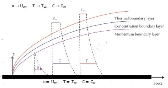
Figure 1.
Geometry of the flow phenomena.
Subject to the boundary conditions
where and are, respectively, horizontal and vertical components of velocity, is the temperature of the fluid, is the kinematic viscosity, is the time constant, is the electrical conductivity, is the thermal diffusivity, is Brownian diffusion coefficients, is thermophoresis coefficient, is the ambient temperature of the fluid, is the temperature of the wall, is the concentration at the wall, is the ambient concentration and is the reaction rate parameter.
In this study, the following transformations are considered to reduce Equations (1)–(5) into a set of dimensionless equations
By substituting transformations (6) into Equations (1)–(5) yields the dimensionless equations of the form
Subject to the dimensionless boundary conditions
where is the Wiesenberg number, is the magnetic parameter, denotes local electric parameter, is the Prandtl number, is the Schmidt number, is the Eckert number, represents thermophoresis parameter, denotes the Brownian motion parameter, and shows the dimensionless reaction rate parameter and these are defined as
3. Finite Element Method
Equations (7)–(10) are solved using a numerical technique based on the Galerkin finite element method. To apply this method for a reduced system of Equations (7)–(10), the whole infinite domain is considered to be finite, . Divide this entire domain into a finite number of subdomains known as finite elements. Since there is only one independent variable in the problem, each element is a line segment with two nodes at both ends. Let and are two nodal coordinates at the left and right node of element, respectively. The nodal variables and are nodal variables assigned to the left and right nodes of element, respectively. Let the length of each element be denoted by . The trial function, which is linear polynomials, is expressed as:
where Equation (7) is reduced into a system of the following two differential equations
By using both nodes of element, the trail function can be expressed as:
The shape functions and are expressed as:
The shape function satisfies the following two properties
i.e., gives the value 1 on the left node and 0 on the right node of element and similarly has the same characteristic. The second property states that the sum of all functions on every node of each element is unity,
For finding approximate numerical solutions of considered boundary value problems using the Galerkin finite element method, weighted residuals of Equations (7)–(9) are constructed first by multiplying test functions to Equations (7)–(9) and integrated it into the entire domain, which gives
Equations (18)–(20) are strong forms. Since weak formulations impose fewer conditions for the existence of derivative(s) on test and trial functions, so weak forms will be constructed. For second-order differential equations, the second-order term will be dropped out if interpolation is carried out using linear polynomials. If small-sized elements are also used, then the method converges to the accurate solution using weak formulation. The solution space is Sobolev space. See the Appendix A for more details on weak formulation. The solution also cannot be found using strong forms. To do so, Equations (18)–(20) are integrated once and it produces
Integrals (17) and (21)–(23) are considered on the whole domain. Now, for the element, these integrals are given as
The nonlinear terms in Equations (25)–(27) are linearized as:
By substituting test and trial functions in Equations (24)–(27), the following matrix-vector equation is obtained
denote matrices of order and denote vector having four entries and each is defined as:
The remaining matrices , are zero matrices, and the rest of the vectors are zero vectors.
The boundary conditions on the leftmost node for Equations (8), (9) and (13) can be employed as
After assembling the matrices, the boundary condition on the rightmost node of Equations (8) and (9) can be expressed similarly.
To define the skin friction coefficients, local Nusselt number, and Sherwood number, we use the following formulae:
where , and .
The dimensionless forms of Skin friction coefficients, local Nusselt and Sherwood numbers are given as:
To clarify the results, a comparison of the local Nusselt number obtained by the considered approach of the modified finite element method is made with those given in past research. It is displayed in Table 1. It is to be noted that the modified approach of the finite element method is considered that has been given/proposed in [44]. Using this approach, finite difference formulas can be considered to compute the derivatives of solutions more accurately if the linear polynomials perform the interpolation. The code can also be validated by looking at the results in Table 2. The Matlab solver bvp4c is also adopted to compute the results. This solver can be used to find solutions to boundary value problems and gives fourth or fifth order of accuracy.

Table 1.
Comparison of present results with those given in past research for calculating the numerical values of using .
Table 2.
Mesh sensitivity test for with varying numbers of elements/nodes using .
4. Results and Discussions
The finite element approach is used to solve the reduced system of boundary value problems. The method is based on the Galerkin weighted residual approach, and integrals are constructed and computed numerically in the computational code. The three points Gauss–Legendre formula is applied to find integrals. Numerical integrals have the advantage over exact analytical integrals in time consumption. The integral formulas contain the three points and three weights. The three points are just roots of the third-degree Legendre polynomial. An iterative method checks the absolute difference between the current and previous solutions at all grid points. If this difference stays smaller than some given tolerance, the iterative method will be stopped; otherwise, it will continue. The iterative method is compulsory for handling nonlinear terms in given differential equations. The nonlinear terms in the equations are linearized first, and further, these are tackled by the iterative method.
Figure 2 shows the mesh considered for applying the finite element method. Since the domain for one-dimensional ODEs is a real line, the domain is infinite, but a finite domain is considered for numerical purposes. As mentioned earlier, the used elements are line segments; therefore, the used mesh is a collection line segment. The variable in Figure 2 shows the variables used in the reduced system of ODEs to be solved.
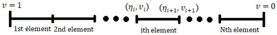
Figure 2.
1D mesh for finite element method.
Figure 3 shows the Wiesenberg number and electric parameter variation on the velocity profile. Velocity decreases by incrementing the Wiesenberg number and grows by enhancing the electric parameter. The growth in the Wiesenberg number is responsible for decreasing the fluid’s viscosity, which leads to enhancement in the resistance of the deformation in the fluid flow; therefore velocity profile decays. Figure 4 shows the effect of the Eckert number and Prandtl number on the temperature profile. The temperature profile rises and decays by enhancing the Eckert and Prandtl numbers, respectively. The temperature profile growth results from an increment in the transformation of work into heat. The escalation in the Prandtl number also produces decay in the thermal diffusivity; consequently, thermal conductivity reduces, and the temperature profile falls. The effect of thermophoresis and Brownian motion parameters on the temperature profile is depicted in Figure 5. The temperature profile is boosted by rising thermophoresis and Brownian motion parameters. Since the hot particles get scattered in the fluid due to an upsurge of random movement, the temperature profile accelerates. The increment in the thermophoresis parameter yields growth in the cycle of shifting particles from the plate to its vicinity, thus increasing temperature profile upturns. Figure 6 illustrates the consequence of the Schmidt number and dimensionless rate parameter in the concentration profile. Temperature profile declines by accumulating Schmidt numbers and dimensionless reaction rate parameters. The augmentation in the Schmidt number offers a decline in mass diffusivity and, consequently, concentration profile falloffs. Since breaking or forming chemical bonds between atoms intensifies due to the augmentation of reaction rate parameters, the concentration profile declines. Figure 7 demonstrates the influence of thermophoresis and Brownian motion parameters on the concentration profile. Concentration profile falloffs and augments by aggregating the thermophoresis and Brownian motion parameters, respectively. Since increments in the Brownian motion, the parameter brings the particles to their vicinity, so particles of concentration also spread randomly, and consequently, the concentration profile rises.
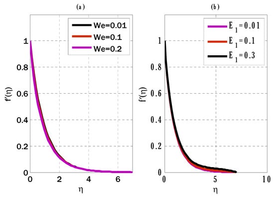
Figure 3.
Variation of Wiesenberg number and electric parameter on velocity profile using . .
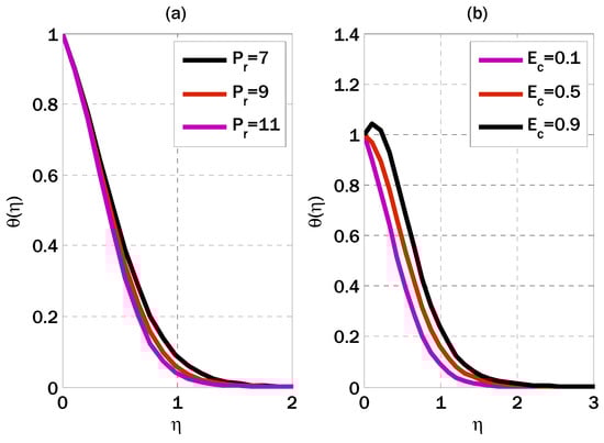
Figure 4.
Variation of Eckert number and Prandtl number on temperature profile using .
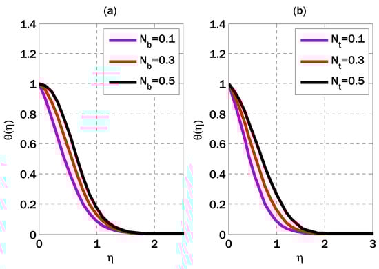
Figure 5.
Variation of thermophoresis and Brownian motion parameters on temperature profile using .
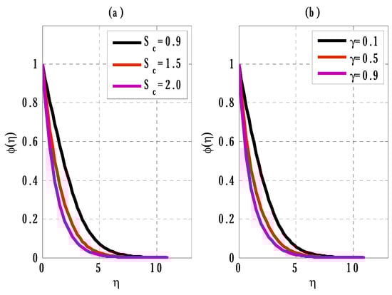
Figure 6.
Variation of Schmidt number and reaction rate parameter on temperature profile using .
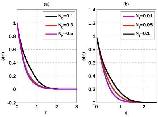
Figure 7.
Variation of thermophoresis and Brownian motion parameters on concentration profile using .
Figure 8 is drawn using the software COMSOL 4.4 which applies the finite element method to solve governing equations of the flow phenomenon. That software requires geometry, types of forces, and boundary conditions. Using this software, heat transfer in Newtonian fluid over a moving plate is studied, and simulations are provided. Figure 8, Figure 9 and Figure 10 include the surface plot of velocity, streamlines, the surface plot temperature, and isothermal contours. The influence of moving velocities of the plate on velocity and temperature profile is depicted in Figure 8, Figure 9 and Figure 10.
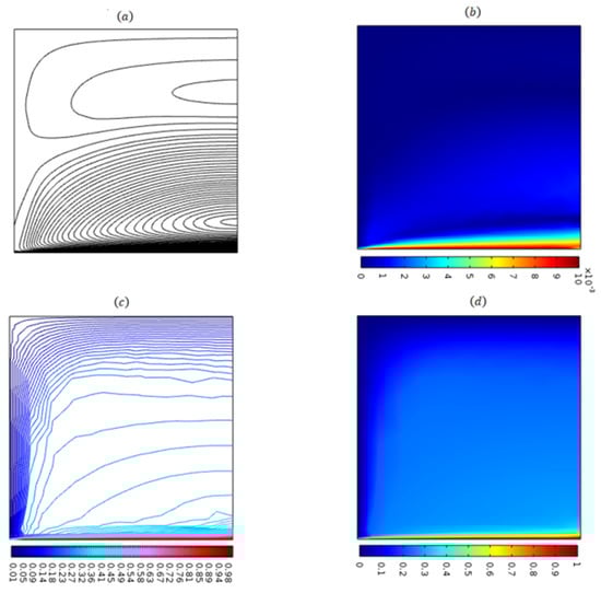
Figure 8.
(a) Surface plot of velocity, (b) streamlines, (c) surface plot of temperature, and (d) isothermal contours using .
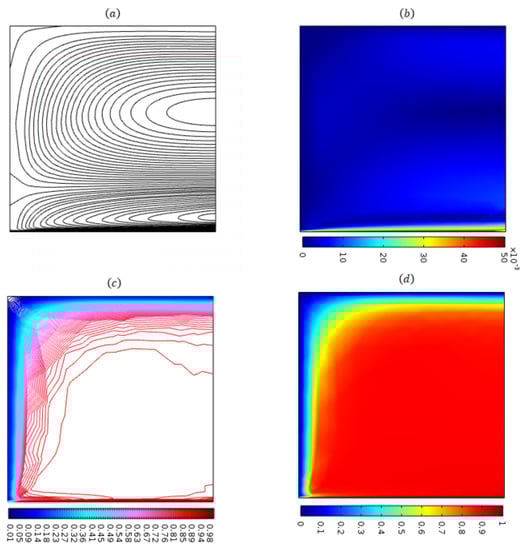
Figure 9.
(a) Surface plot of velocity, (b) streamlines, (c) surface plot of temperature, and (d) isothermal contours using .
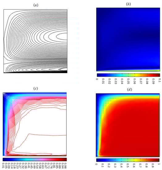
Figure 10.
(a) Surface plot of velocity, (b) streamlines, (c) surface plot of temperature, and (d) isothermal contours using .
Table 3 shows the numerical values of the skin friction coefficient (excluding Reynolds number) by varying magnetic parameters, electric parameters, and Wiesenberg number. The skin friction coefficient heightens by enhancing the magnetic parameter and Wiesenberg number while it decays by raising the electric parameter. The growth in magnetic parameter yields decays in the velocity profile, so friction at the plate rises, and therefore skin friction coefficient augments. The enhancement of the electric parameter results in an escalation in velocity profile, leading to growth in the friction at the plate and, therefore, the skin friction coefficient rises. Table 4 appearances the consequence of the thermophoresis parameter, Brownian motion parameter, electric parameter, and Prandtl number on the local Nusselt number (excluding Reynolds number). The local Nusselt number declines by mounting thermophoresis, Brownian motion, and electric parameters while it enhances by a rising Prandtl number. Table 5 displays the effect of the Schmidt number and reaction rate parameter on the local Sherwood number (excluding the Reynolds number). The local Sherwood number rises as the Schmidt number and dimensionless reaction rate parameter increase.
Table 3.
List of numerical values for skin friction coefficient.
Table 4.
List of numerical values for the local Nusselt number using .
Table 5.
List of numerical values of the local Sherwood number using .
5. Conclusions
This work was to investigate the non-Newtonian nanofluid flow under the effect of heat and mass transfer, viscous dissipation, and chemical reaction. The governing equations have been reduced into linear and nonlinear boundary value problems and solved with the finite element method with an iterative procedure. Some of the results were also obtained by Matlab solver bvp4c. We observed that the FEM simulation results agree very well with bvp4c and published data. The solver produced fourth or fifth-order accurate results. The problem of Newtonian fluid over a moving plate is solved with software that applies the finite element method. The results were obtained by varying velocities of the plate. These final thoughts can be stated as:
- The decline in the velocity profile was brought about by increasing the electrical parameters.
- As Eckert’s number increased, so did the temperature profile.
- Growing the thermophoresis parameter decreased the concentration profile.
In addition, nonlinear problems of a similar nature that arise in computational fluid dynamics can be quickly solved using the finite element method presented here. After this project is finished, further uses for the current approach can be suggested [47,48,49,50]. The suggested method is not only simple to implement, but it also solves a more general class of differential equations.
Author Contributions
Conceptualization, methodology, and analysis, Y.N.; funding acquisition, W.S.; investigation, Y.N.; methodology, M.S.A.; project administration, W.S.; resources, W.S.; supervision, M.S.A.; visualization, W.S.; writing—review and editing, M.S.A.; proofreading and editing, M.S.A. All authors have read and agreed to the published version of the manuscript.
Funding
The authors would like to acknowledge the support of Prince Sultan University for providing the Article Processing Charges (APC) of this publication.
Data Availability Statement
The manuscript included all required data and implementing information.
Acknowledgments
The authors wish to express their gratitude to Prince Sultan University for facilitating the publication of this article through the Theoretical and Applied Sciences Lab.
Conflicts of Interest
The authors declare no conflict of interest.
Nomenclature
| horizontal components of velocity | |
| Cartesian co-ordinate | |
| kinematic viscosity | |
| density of fluid | |
| concentration of fluid | |
| Brownian diffusion coefficient | |
| specific heat capacity | |
| strength of electric field | |
| reaction rate | |
| reaction rate parameter | |
| time constant (s) | |
| magnetic parameter | |
| Prandtl number | |
| Brownian motion variable | |
| electrical conductivity of the fluid | |
| temperature of fluid | |
| temperature of fluid at the wall | |
| ambient temperature of the fluid | |
| concentration on the wall | |
| ambient concentration | |
| strength of imposed transverse magnetic field | |
| thermal diffusivity | |
| dynamic viscosity | |
| effective heat capacity of fluid | |
| Eckert number | |
| thermophoresis variable | |
| Schmidt number |
Appendix A
Three different weak formulations correspond to velocity, temperature, and concentration profile. For the weak formulation of the velocity profile, assume that there exists constant such that and for all .
Definition A1.
Let the triplet is a weak solution of boundary value problems (13) and (8) and (9) if the Equations (21)–(23) hold, where and is the Sobolev space.
Theorem A1.
By using assumption and , the following results hold.
Proof.
Let such that
where it is defined that
Since is an orthonormal basis of so it gives
Multiplying (A1) by and add the result for
This implies
□
References
- Alfven, H. Existence of electromagnetic-hydrodynamic waves. Nature 1942, 150, 405–406. [Google Scholar] [CrossRef]
- Hartmann, J.; Hg-Dynamics, I. Theory of the laminar flow of an electrically conducting liquid in a homogeneous magnetic field. K. Dan. Vidensk. Selsk. Mat.-Fys. Medd. 1937, 15, 1–27. [Google Scholar]
- Rashidi, M.M.; Abelman, S.; Mehr, N.F. Entropy generation in steady MHD flow due to a rotating disk in a nanofluid. Int. J. Heat Mass Transf. 2013, 62, 515–525. [Google Scholar] [CrossRef]
- Shehzad, S.A.; Alsaedi, A.; Hayat, T. Hydromagnetic steady flow of Maxwell fluid over a bidirectional stretching surface with prescribed surface temperature and prescribed surface heat flux. PLoS ONE 2013, 8, e68139. [Google Scholar] [CrossRef] [PubMed]
- Turkyilmazoglu, M. Exact solutions for the incompressible viscous magnetohydrodynamic fluid of a rotating disk flow. Int. J. Nonlinear Mech. 2011, 46, 306–311. [Google Scholar] [CrossRef]
- Hayat, T.; Shehzad, S.A.; Ashraf, M.B.; Alsaedi, A. Magneto hydrodynamic mixed convection flow of thixotropic fluid with thermophoresis and Joule heating. J. Thermophys. Heat Transf. 2013, 27, 733–740. [Google Scholar] [CrossRef]
- Dandapat, B.S.; Mukhopadhyay, A. Finite amplitude long wave instability of a film of conducting fluid flowing down an inclined plane in presence of electromagnetic field. Int. J. Appl. Mech. Eng. 2003, 8, 379–383. [Google Scholar]
- Sheikholeslami, M.; Gorji-Bandpay, M.; Ganji, D.D. Magnetic field effects on natural convection around a horizontal circular cylinder inside a square enclosure filled with nanofluid. Int. Commun. Heat Mass Transf. 2012, 39, 978–986. [Google Scholar] [CrossRef]
- Hayat, T.; Shafiq, A.; Nawaz, M.; Alsaedi, A. MHD axisymmetric flow of third grade fluid between porous disks with heat transfer. Appl. Math. Mech. 2012, 33, 749–764. [Google Scholar] [CrossRef]
- Ahmad, K.; Nazar, R. Unsteady magnetohydrodynamic mixed convection stagnation point flow of a viscoelastic fluid on a vertical surface. JQMA 2010, 6, 105–117. [Google Scholar]
- Hatami, M.; Sheikholeslami, M.; Hosseini, M.; Ganji, D.D. Analytical investigation of MHD nanofluid flow in non-parallel walls. J. Mol. Liq. 2014, 194, 251–259. [Google Scholar] [CrossRef]
- Sheikholeslami, M.; Ganji, D.D.; Gorji-Bandpy, M.; Soleimani, S. Magnetic field effect on nanofluid flow and heat transfer using KKL model. J. Taiwan Inst. Chem. Eng. 2014, 45, 795–807. [Google Scholar] [CrossRef]
- Abolbashari, M.H.; Freidoonimehr, N.; Nazari, F.; Rashidi, M.M. Entropy analysis for and unsteady MHD flow past a stretching permeable surface in nanofluid. Powder Technol. 2014, 267, 256–267. [Google Scholar] [CrossRef]
- Rashidi, M.M.; Erfani, E. Analytical method for solving steady MHD convective and slip flow due to a rotating disk with viscous dissipation and Ohmic heating. Eng. Comput. 2012, 29, 562–579. [Google Scholar] [CrossRef]
- Rashidi, M.M.; Ali, M.; Freidoonimehr, N.; Rostami, B.; Hossain, M.A. Mixed convective heat transfer for MHD viscoelastic fluid flow over a porous wedge with thermal radiation. Adv. Mech. Eng. 2014, 10, 735939. [Google Scholar] [CrossRef]
- Bhattacharyya, K.; Mukhopadhyay, S.; Layek, G.C.; Pop, I. Effects of thermal radiation on micropolar fluid flow and heat transfer over a porous shrinking sheet. Int. J. Heat Mass Transf. 2012, 55, 2945–2952. [Google Scholar] [CrossRef]
- Makinde, O.D.; Ogulu, A. The effect of thermal radiation on the heat and mass transfer flow of a variable viscosity fluid past a vertical porous plate permeated by a transverse magnetic field. Chem. Eng. Commun. 2008, 195, 1575–1584. [Google Scholar] [CrossRef]
- Hayat, T.; Shafiq, A.; Alsaedi, A. Effect of Joule heating and thermal radiation in flow of third-grade fluid over radiative surface. PLoS ONE 2014, 9, e83153. [Google Scholar] [CrossRef] [PubMed]
- Motsumi, T.G.; Makinde, O.D. Effects of thermal radiation and viscous dissipation on boundary layer flow of nanofluids over a permeable moving flat plate. Phys. Scr. 2012, 86, 045003. [Google Scholar] [CrossRef]
- Makinde, O.D. MHD mixed-convection interaction with thermal radiation and nth order chemical reaction past a vertical porous plate embedded in a porous medium. Chem. Eng. Commun. 2011, 198, 590–608. [Google Scholar] [CrossRef]
- Shehzad, S.A.; Alsaedi, A.; Hayat, T.; Alhuthali, M.S. Thermophoresis particle deposition in mixed convection threedimensional radiative flow of an Oldroyd-B fluid. J. Taiwan Inst. Chem. Eng. 2014, 45, 787–794. [Google Scholar] [CrossRef]
- Sakiadis, B.C. Boundary layer behaviour on continuous moving solid surfaces. I. Boundary layer equations for two-dimensional and axisymmetric flow. II. Boundary layer on a continuous flat surface. iii. boundary layer on a continuous cylindrical surface. Am. Inst. Chem. Eng. J. 1961, 7, 26–28. [Google Scholar] [CrossRef]
- Crane, L.J. Flow past a stretching sheet. Z. Appl. Math. Phys. 1970, 21, 645–647. [Google Scholar]
- Gupta, P.S.; Gupta, A.S. Heat and mass transfer on a stretching sheet with suction or blowing. Can. J. Chem. Eng. 1977, 55, 744–746. [Google Scholar] [CrossRef]
- Abd El-Aziz, M. Radiation effect on the flow and heat transfer over an unsteady stretching sheet. Int. Commun. Heat Mass Transf. 2009, 36, 521–524. [Google Scholar] [CrossRef]
- Elbashbeshy, E.M.A. Heat transfer over a stretching surface with variable surface a heat flux. J. Phys. D Appl. Phys. 1998, 31, 1951–1954. [Google Scholar] [CrossRef]
- Mukhopadyay, S. Effect of thermal radiation on unsteady mixed convection flow and heat transfer over a porous stretching surface in porous medium. Int. Commun. Heat Mass Transf. 2009, 52, 3261–3265. [Google Scholar] [CrossRef]
- Shateyi, S.; Motsa, S.S. Thermal radiation effects on heat and mass transfer over an unsteady stretching surface. Math. Probl. Eng. 2009, 2009, 965603. [Google Scholar] [CrossRef]
- Abd El-Aziz, M. Thermal-diffusion and diffusion-thermo effects on combined heat and mass transfer by hydromagnetic threedimensional free convection over a permeable stretching surface with radiation. Phys. Lett. 2007, 372, 263–272. [Google Scholar] [CrossRef]
- Hady, F.M.; Ibrahim, F.S.; Abdel-Gaied, S.M.; Eid, M.R. Radiation effect on viscous flow of a nanofluid and heat transfer over a nonlinearly stretching sheet. Nanoscale Res. Lett. 2012, 7, 229. [Google Scholar] [CrossRef] [PubMed]
- Pavlov, K.B. Magnetohydromagnetic flow of an incompressible viscous fluid caused by deformation of a surface. Magn. Gidrodin. 1974, 4, 146–148. [Google Scholar]
- Bianco, V.; Manca, O.; Nardini, S. Second law analysis of Al2O3 water nanofluid turbulent forced convection in a circular cross section tube with constant wall temperature. Adv. Mech. Eng. 2013, 203, 920278. [Google Scholar] [CrossRef]
- Nadeem, S.; Haq, R.U.; Akbar, N.S.; Khan, Z.H. MHD three dimensional Casson fluid flow past a porous linearly stretching sheet. Alex. Eng. J. 2013, 52, 577–582. [Google Scholar] [CrossRef]
- Akbar, N.S.; Haq, R.U.; Nadeem, S. Study of Williamson nanofluid flow in an symmetric channel. Res. Phys. 2013, 3, 161–166. [Google Scholar]
- Elbashbeshy EM, A.; Bazid, M.A. Heat transfer over an unsteady stretching surface with internal heat generation. Appl. Math. Comput. 2003, 138, 239–245. [Google Scholar] [CrossRef]
- Shafiq, A.; Çolak, A.B.; Sindhu, T.N.; Al-Mdallal, Q.M.; Abdeljawad, T. Estimation of unsteady hydromagnetic Williamson fluid flow in a radiative surface through numerical and artificial neural network modeling. Sci. Rep. 2021, 11, 14509. [Google Scholar] [CrossRef]
- Rizk, D.; Ullah, A.; Elattar, S.; Alharbi, K.A.M.; Sohail, M.; Khan, R.; Khan, A.; Mlaiki, N. Impact of the KKL Correlation Model on the Activation of Thermal Energy for the Hybrid Nanofluid (GO+ZnO+Water) Flow through Permeable Vertically Rotating Surface. Energies 2022, 15, 2872. [Google Scholar] [CrossRef]
- Suganya, S.; Muthtamilselvan, M.; Al-Amri, F.; Abdalla, B. An exact solution for unsteady free convection flow of chemically reacting Al2O3–SiO2/water hybrid nanofluid. Proc. Inst. Mech. Eng. Part C J. Mech. Eng. Sci. 2021, 235, 3749–3763. [Google Scholar] [CrossRef]
- Saeed, A.; Alghamdi, W.; Mukhtar, S.; Shah, S.I.A.; Kumam, P.; Gul, T.; Nasir, S.; Kumam, W. DarcyForchheimer hybrid nanofluid flow over a stretching curved surface with heat and mass transfer. PLoS ONE 2021, 16, e0249434. [Google Scholar] [CrossRef]
- Gul, T.; Noman, W.; Sohail, M.; Khan, M.A. Impact of the Marangoni and thermal radiation convection on the graphene-oxide-water-based and ethylene-glycol-based nanofluids. Adv. Mech. Eng. 2019, 11, 1687814019856773. [Google Scholar] [CrossRef]
- Abbas, A.; Jeelani, M.B.; Alnahdi, A.S.; Ilyas, A. MHD Williamson Nanofluid Fluid Flow and Heat Transfer Past a Nonlinear Stretching Sheet Implanted in a Porous Medium: Effects of Heat Generation and Viscous Dissipation. Processes 2022, 10, 1221. [Google Scholar] [CrossRef]
- Gul, T.; Khan, M.A.; Noman, W.; Khan, I.; Abdullah Alkanhal, T.; Tlili, I. Fractional order forced convection carbon nanotube nanofluid flow passing over a thin needle. Symmetry 2019, 11, 312. [Google Scholar] [CrossRef]
- Hayat, T.; Shafiq, A.; Alsaedi, A. Hydromagnetic boundary layer flow of Williamson fluid in the presence of thermal radiation and Ohmic dissipation. Alex. Eng. J. 2016, 55, 2229–2240. [Google Scholar] [CrossRef]
- Nawaz, Y.; Arif, M.S. An effective modification of finite element method for heat and mass transfer of chemically reactive unsteady flow. Comput. Geosci. 2020, 24, 275–291. [Google Scholar] [CrossRef]
- Khan, W.A.; Pop, I. Boundary layer flow of a nanofluid past a stretching sheet. Int. J. Heat Mass Transfer 2010, 53, 2477–2483. [Google Scholar] [CrossRef]
- Srinivasulu, T.; Goud, B.S. Effect of inclined magnetic field on flow, heat and mass transfer of Williamson nanofluid over a stretching sheet. Case Stud. Therm. Eng. 2021, 23, 100819. [Google Scholar] [CrossRef]
- Bibi, M.; Nawaz, Y.; Arif, M.S.; Abbasi, J.N.; Javed, U.; Nazeer, A. A finite difference method and effective modification of gradient descent optimization algorithm for MHD fluid flow over a linearly stretching surface. Computers. Mater. Contin. 2020, 62, 657–677. [Google Scholar]
- Arif, M.S.; Bibi, M.; Jhangir, A. Solution of algebraic lyapunov equation on positive-definite hermitian matrices by using extended Hamiltonian algorithm. Comput. Mater. Contin. 2018, 54, 181–195. [Google Scholar]
- Pasha, S.A.; Nawaz, Y.; Arif, M.S. A third-order accurate in time method for boundary layer flow problems. Appl. Numer. Math. 2021, 161, 13–26. [Google Scholar] [CrossRef]
- Nawaz, Y.; Arif, M.S. Modified class of explicit and enhanced stability region schemes: Application to mixed convection flow in a square cavity with a convective wall. Int. J. Numer. Methods Fluids 2021, 93, 1759–1787. [Google Scholar] [CrossRef]
Disclaimer/Publisher’s Note: The statements, opinions and data contained in all publications are solely those of the individual author(s) and contributor(s) and not of MDPI and/or the editor(s). MDPI and/or the editor(s) disclaim responsibility for any injury to people or property resulting from any ideas, methods, instructions or products referred to in the content. |
© 2023 by the authors. Licensee MDPI, Basel, Switzerland. This article is an open access article distributed under the terms and conditions of the Creative Commons Attribution (CC BY) license (https://creativecommons.org/licenses/by/4.0/).