Article

External Identification of a Reciprocal Lossy Multiport Circuit under Measurement Uncertainties by Riemannian Gradient Descent

1
Dipartimento di Ingegneria dell’Informazione, Università Politecnica delle Marche (UPM), Via Brecce Bianche, I-60131 Ancona, Italy
2
School of Information, Beijing Wuzi University, Fuhe Street, Tongzhou District, Beijing 101149, China
*
Author to whom correspondence should be addressed.
Energies 2023, 16(6), 2585; https://doi.org/10.3390/en16062585
Submission received: 4 February 2023 / Revised: 2 March 2023 / Accepted: 6 March 2023 / Published: 9 March 2023
(This article belongs to the Section F: Electrical Engineering)

Abstract

:
The present paper deals with the external identification of a reciprocal, special passive, 2 n -port network under measurement uncertainties. In the present context, the multiport model is represented by an admittance matrix and the condition that the network is ‘reciprocal special passive’ refers to the assumption that the real part of the admittance matrix is symmetric and positive-definite. The key point is to reformulate the identification problem as a matrix optimization program over the matrix manifold S + ( 2 n ) × S ( 2 n ) . The optimization problem requires a least-squares criterion function designed to cope with over-determinacy due to the incoherent data pairs whose cardinality exceeds the problem’s number of degrees of freedom. The present paper also proposes a numerical solution to such an optimization problem based on the Riemannian-gradient steepest descent method. The numerical results show that the proposed method is effective as long as reasonable measurement error levels and problem sizes are being dealt with.

1. Introduction

Two-port and multiport circuits are frequently employed in engineering and in applied sciences to model complex circuit portions. Multiport circuit models are not limited to electrical phenomena. For instance, multiport models have been used in the modeling of acoustic systems [1] and transducers [2]; in the analysis of mufflers of complex geometry [3]; in the analysis of power delivery in electrical railways systems [4]; in the analysis of microvascular networks [5]; in the characterization of hydraulic systems [6]; in waveguide calibration [7]; in the modeling of electrochemical transport processes through biological membranes [8]; in the analysis of harmonic-chain-based energy harvesters [9]; in the design of wireless power transfer systems [10,11]; in the representation of electro-mechanical transducers [12]; in the simulation of bending magnets [13]; in the modeling of complex mechanical systems [14]; and in the design of power converter configurations for grid-connected photovoltaic systems [15].
Most modeling techniques involve two-port models. However, multiport circuit models are of prime importance in representing linear interaction phenomena where a large number of variables are involved. As a specific application, to exemplify the usefulness of multiport identification, consider the electronic chip-package de-embedding problem. This problem was tackled for a three-port network in [16] and for a general n-port network in [17]. The plastic package/connector of semiconductor-based electronic chips embeds a number of highly conductive wires whose function is to connect the internal electronic chip to the external pins. At very high frequencies (in the range of GHz), a number of parasitic effects appear and the wires electromagnetically interact with one another in such a way that they may no longer be regarded as simple wires. Therefore, it is of prime importance to obtain an accurate mathematical model of such interactions in order to recover the original signals from the mixed ones.
In [17], the electronic chip package was modeled as a reciprocal, linear, time-invariant multiport network, which is supposed to be accessible using n internal electrical ports and n external electrical ports. The identification of the model, represented through a 2 n × 2 n admittance matrix Y, may be carried out by measuring the admittance of the external ports using a vector network analyzer. (Network analyzers are often used to characterize two-port networks such as amplifiers and filters, but they can be used to characterize networks with an arbitrary number of ports. The basic architecture of a network analyzer involves a signal generator, a test set, one or more receivers and a display. Most vector network analyzers have two test ports, permitting the measurement of four parameters, but instruments with more than two ports are commercially available). The internal ports are connected to specific known loads, termed ‘standards’. In order to save time, the number of standards may be kept to a minimum; however, this requires the measurements to be extremely precise.
On the basis of the current knowledge of system modeling by multiport circuits and their external identification, the present contribution proposes a novel technique to determine the entries of the admittance matrix Y (in the frequency domain) in the presence of measurement errors by setting up a non-linear optimization problem. In particular, we contribute to the mathematical treatment of the problem by assuming that an arbitrary number of standards may be accessed and that such measures may be affected by uncertainties. Moreover, we add the assumption that the sought multiport network is energetically passive, which makes the modeling problem manifold-structured and calls for a Riemannian-gradient optimization of a properly designed criterion function.
A key feature of the present contribution is that modeling is formulated as an optimization program over a product-manifold, obtained using the product of the set of real symmetric, positive-definite matrices and by the set of real symmetric matrices. One such formulation can be used to deal with the physical constraints that a model needs to obey and with the numerical optimization process carried out by a computer-based implementation of a Riemannian-gradient steepest-descent method. We note that the interplay between multiport systems and geometric (Hamiltonian) systems was investigated in the literature (see, for instance, the introductory survey [18]).
The present research paper is organized as follows. In Section 2, we recall the general equations pertaining to a multiport model when half of the ports are closed on known loads and the remaining half are subjected to measurements. In particular, Section 2.3 and Section 2.4 explain the technical assumptions regarding the sought model and the known-loads, which result in mathematical constrains on the optimization problem laid out in Section 2.5. This was set up to formulate the identification problem under measurement uncertainties and redundant measurements. Section 3 presents a Riemannian-gradient-based algorithm to estimate the optimal parameters of the sought multiport model; Section 3.1 defines the optimization criterion function and illustrate the calculation of its Riemannian gradients in detail with respect to the real part and imaginary part of the sought admittance matrix representing the multiport model; Section 3.2 presents the optimization algorithm in terms of a geodesic stepping method on the product manifold S + ( 2 n ) × S ( 2 n ) . Section 4 illustrates the results of a number of numerical experiments aiming to assess the numerical features of the devised numerical optimization method during the identification of an unknown multiport system. The Section 5 provides some final remarks.

2. Problem Formulation

To formulate the problem at hand, we shall make use of a linear circuit-theoretic notation. However, the mathematical formulation is context-independent as it essentially boils down to a non-linear, structured, complex-valued matrix optimization problem. For an introduction to linear circuit theory and matrix-based representations, readers might consult, e.g., [19].

2.1. Linear, Time-Invariant Multiport Model

We assume that a linear, time-invariant (LTI) multiport system is partitioned into n internal ports, described by a Fourier-domain current/voltage vector-pair ( I I , V I ) and n external port described by a Fourier-domain vector-pair ( I E , V E ) , therefore, it holds that I I , V I , I E , V E C n . In applied fields other than pure circuit theory, a current/voltage pair may be replaced by any pair of conjugate variables, such as ionic-current/electrochemical-potential in biochemistry (see, e.g., Equations (1) and (2) in [8]) or blood-flow-rate/blood-pressure in circulatory physiology (see, e.g., the review in [20]).
The LTI 2 n -port system is supposed to possess an admittance-matrix representation, namely:
I E I I = Y EE Y EI Y IE Y II = : Y V E V I ,
where the four blocks Y EE , Y EI , Y IE and Y II of the complex-valued 2 n × 2 n admittance matrix Y belong to C n × n . In the present research paper, we adopt the following standpoints:
  • In principle, the behavior of the multiport system depends on the frequency of the excitation; assuming that the system is linear and time-invariant, it is possible to appeal to the Fourier theory and work with one frequency at a time (in other terms, phasor theory is in force);
  • While a two-port network admits one or more of six independent matrix representations (impedance, admittance, scattering, inverse scattering, hybrid, inverse hybrid), a multiport network admits one or more amid a large number of representations, among which only four (impedance, admittance, scattering, inverse scattering) are univocally determined, while the hybrid representations are multiple. The scattering-matrix representations are popular in waveguide theory, while impedance/admittance-matrix representations are common in electrical engineering; in the present paper, we will only consider multiport networks that admit both impedance and admittance representations.
Assume that multiple loads of known admittance are connected to each of the internal ports. The constraints on the internal electrical variables read:
I I = Y S V I ,
where Y S C n × n represents the admittance matrix of the load (namely, it represents a standard).
The n-port system arising by connecting the internal ports of the 2 n -port network to a n-port standard behaves, in turn, as a n-port, which is described by the admittance matrix Y M C n × n , that links the external variables by I E = Y M V E . The admittance matrix Y M may be measured by a vector network analyzer (see, for example, reference [21] for the case of wave-guides). Combining the relationship (2) with the relationship (1), we obtain:
Y M = Y EE Y EI ( Y S + Y II ) 1 Y IE ,
which is well-defined only if det ( Y S + Y II ) 0 .
Example 1. 
Ideally, the admittance matrix Y S will be diagonal and each known-load will be realized as a resistive-capacitive impedance (coils are cumbersome, while capacitors are easy to miniaturize). In practice, especially at high frequencies, it is impossible to realize the independence of the loads across the internal ports; therefore, the matrix Y S is assumed to be non-diagonal (albeit possibly diagonal-dominant). The presence of non-zero off-diagonal terms indicates the coupling of the sub-loads.

2.2. Model Identification under the Assumption of Perfect Measurements

In the research paper [17], it is assumed that the 2 n -port network representing the electronic chip package/connector is reciprocal, implying the symmetry of the admittance matrix Y; namely, that Y EE = Y EE , Y II = Y II and Y IE = Y EI , where the superscript denotes matrix transposition. As a consequence, the Equation (3) simplifies into
Y M = Y EE Y EI ( Y S + Y II ) 1 Y EI .
Likewise, the standard load is assumed to be represented by a reciprocal multiport circuit, which implies that matrix Y S is also symmetric. A reciprocal n-port standard connected to a reciprocal 2 n -port network results in a reciprocal n-port network which, in turn, implies that the matrix Y M is also symmetric.
The multiport identification problem under the assumption of error-free measurements may be summarized as follows: Assuming that the admittance matrices Y S ( k ) C n × n , k = 0 , 1 , , 4 , of five standards and the admittance matrices Y M ( k ) C n × n , k = 0 , 1 , , 4 of five corresponding measurements at the external pins of the electronic chip package/connector are available, the three matrix blocks Y EE , Y EI and Y II that perfectly fit the data can be found. Le us recall the closed-form solution proposed in [17].
A canonical way to obtain the submatrix Y EE is to measure the admittance matrix Y M that corresponds to short-circuited internal ports. In fact, if all the internal ports are short-circuited, it holds that Y S ( 0 ) = and, therefore, that Y EE = Y M ( 0 ) .
To determine the other two submatrices Y II and Y EI , let us set up the system of matrix equations
Y M ( k ) = Y EE Y EI ( Y S ( k ) + Y II ) 1 Y EI , k = 0 , 1 , , 4 .
The unknown block Y II can be expressed as a function of the unknown block Y EI by subtracting the equation in the system (5) corresponding to k = 0 to the equation corresponding to k = 1 , which gives the relationship
Y II = Y EI ( Y M ( 1 ) Y M ( 0 ) ) 1 Y EI Y S ( 1 ) .
Analogously, subtracting the equation corresponding to k = 0 to the equation corresponding to k = 2 , k = 3 and k = 4 , respectively, and plugging in the right-hand side of (6) for Y II , we can obtain the relationships
Z 2 = Y EI Θ 2 Y EI 1 , Z 3 = Y EI Θ 3 Y EI 1 , Z 4 = Y EI Θ 4 Y EI 1 ,
where we made use of the auxiliary matrices
Z k : = ( Y M ( k ) Y M ( 0 ) ) 1 ( Y M ( 1 ) Y M ( 0 ) ) 1 , Θ k : = Y S ( 1 ) Y S ( k ) ,
with k = 2 , 3 , 4 .
After solving for the matrix block Y EI and substituting the found solution in (6), it is possible to recover the submatrix Y II as well. We underline that, in order to achieve a solution using the recalled method, not only are the available measurements supposed to be affected by negligible errors, the sub-block Y EI is supposed to be invertible.
Using the first two equations in (7), we obtain
Z 2 1 Z 3 = Y EI Θ 2 1 Θ 3 Y EI 1 ,
If the matrix Θ 2 1 Θ 3 is diagonalizable, it may be expressed as Θ 2 1 Θ 3 = V Θ Λ V Θ 1 , where the columns of the matrix V Θ C n × n coincide with the eigenvectors of the matrix Θ 2 1 Θ 3 and the matrix Λ is n × n complex-valued diagonal and contains the eigenvalues of the matrix Θ 2 1 Θ 3 . Therefore, we can write
Z 2 1 Z 3 = ( Y EI V Θ ) Λ ( Y EI V Θ ) 1 .
The above equation tells that, if we denote the matrix of the eigenvectors of the product Z 2 1 Z 3 by V Z C n × n , the following relationship holds
V Z = Y EI V Θ Σ ,
where Σ is a n × n complex-valued diagonal unknown matrix that accounts for the fact that the eigenvectors are determined apart from a scaling factor. (This is true if the columns of the matrices V Z and V Θ are ordered by descending eigenvalues moduli; otherwise, we should include an arbitrary permutation matrix to fix any possible arbitrary ordering problem.) By expressing the submatrix Y EI as a function of V Z , V Θ and Σ , we can obtain
Y EI = V Z Σ 1 V Θ 1 ,
and by substituting the right-hand side of this expression in the relationship between Z 2 and Θ 2 in (7), we obtain
Z 2 = V Z T Σ ( V Θ Θ 2 V Θ ) Σ V Z 1 .
Accordingly, the matrix Σ 2 can be recovered from the above relationship since, if the eigenvalues of Θ 2 1 Θ 3 are distinct, then V Θ Θ 2 V Θ is diagonal [22], therefore Σ ( V Θ Θ 2 V Θ ) Σ is a product of diagonal matrices; therefore, it holds that Σ ( V Θ Θ 2 V Θ ) Σ = Σ 2 ( V Θ Θ 2 V Θ ) . Substituting the above relationship into the formula (13), we can obtain
Σ 2 = ( V Z Z 2 V Z ) ( V Θ Θ 2 V Θ ) 1 .
The sign of the in-diagonal entries of the matrix Σ cannot be recovered using the first two equations in (7) since V Θ Θ 2 V Θ and V Θ Θ 3 V Θ are both diagonal [22]. These signs can be determined using the last equation in (7), since Θ 4 cannot be diagonalized by V Θ . Let us set Σ = ± S Σ 2 , with S being a diagonal n × n matrix such that S r r { 1 , + 1 } for r = 1 , 2 , , n . If, in the last equation of (7), we substitute the expression of Y EI as a function of S, we obtain
Z 4 = Y EI T Θ 4 Y EI 1 = V Z T S Σ 2 V Θ Θ 4 V Θ Σ 2 S V Z 1
and, therefore,
V Z Z 4 V Z = S Σ 2 V Θ Θ 4 V Θ Σ 2 S .
Defining D : = V Z Z 4 V Z and B : = Σ 2 V Θ Θ 4 V Θ Σ 2 , the above relationship can be rewritten as D = S B S . Since neither the matrix B nor the matrix D are diagonal, it is now possible to determine one of the two solutions ± S by means of a simple recursion. Since the matrix S is diagonal, it holds that D r s = S r r S s s B r s ; therefore, we can compute the non-zero entries of S using
S 11 : = 1 , S r + 1 , r + 1 = D r , r + 1 S r r B r , r + 1 , for   r = 1 , 2 , , n 1 .
In summary, the complete solution to the multiport identification problem as proposed in [17] is given by:
Y EE = Y M ( 0 ) , Z k = ( Y M ( k ) Y M ( 0 ) ) 1 ( Y M ( 1 ) Y M ( 0 ) ) 1 , k = 2 , 3 , 4 , Θ k = Y S ( 1 ) Y S ( k ) , k = 2 , 3 , 4 , V Z =   eigenvector   matrix   of   Z 2 1 Z 3   ordered   by   descending   eigenvalue   moduli , V Θ =   eigenvector   matrix   of   Θ 2 1 Θ 3   ordered   by   descending   eigenvalue   moduli , Σ 2 = ( V Z Z 2 V Z ) ( V Θ Θ 2 V Θ ) 1 , D = V Z Z 4 V Z , B = Σ 2 V Θ Θ 4 V Θ Σ 2 , S =   result   of   the   iteration   ( 17 ) , Y EI = ± V Z S Σ 2 V Θ 1 , Y II = Y EI ( Y M ( 1 ) Y M ( 0 ) ) 1 Y EI Y S ( 1 ) .
We underline that the above closed-form solution remains valid under a few assumptions, namely, that (1) the matrices Y S ( k ) and Y M ( k ) perfectly agree with the model (4), which implies that their measurement was infinitely precise, and that (2) the eigenvalues of the matrices Z 2 1 Z 3 and Θ 2 1 Θ 3 are distinct. The first assumption does not seem universally realistic and does not hold in inexpensive experimental settings; therefore, we suggest reformulating the problem in a different way to consider this phenomenon, as explained in the following subsections.

2.3. Further Assumptions Regarding the Multiport System

The sought 2 n -port is energetically passive (meaning that it is unable to deliver energy). This hypothesis implies that the matrix Y + Y is positive semi-definite [23] (the superscript denotes conjugate transpose).
Let us explicitly denote the real part and the imaginary part of the complex-valued matrix Y by Y Re and Y Im , respectively (namely Y = Y Re + j Y Im , where j denotes the imaginary unit). The above hypotheses imply that
  • The matrix Y Re (termed conductance matrix) is symmetric and positive definite;
  • The matrix Y Im (termed susceptance matrix) is symmetric.
Let us denote by S ( 2 n ) the space of 2 n × 2 n symmetric matrices and by S + ( 2 n ) the space of 2 n × 2 n symmetric, positive-definite matrices. The above conditions may be stated compactly using the following, suggestive, notation:
Y S + ( 2 n ) + j S ( 2 n ) .
Let us discuss the above technical assumptions by using an example and a counter-example to clarify their physical meaning.
Example 2. 
Let us consider a simple passive reciprocal network and its admittance matrix. Let us consider a π-type two-port network, whose electrical structure is recalled in Figure 1.
Its admittance matrix is Y = G 1 + G 2 G 2 G 2 G 1 + G 2 , where G 1 : = 1 R 1 > 0 and G 2 : = 1 R 2 > 0 . This admittance matrix, which is purely real-valued, is symmetric and positive-definite, and represents a special passive network. (Notice that, in the ideal case where the value of the resistance R 1 is large (hence, the value of the conductance G 1 is small) and the value of the resistance R 2 is small (hence the value of the conductance G 2 is large), the matrix Y is well-balanced and markedly non-diagonal-dominant).
As a counter-example, let us consider a class of multiports that may be energetically passive but are not captured by a strictly positive-definite admittance-matrix representation.
We may speculate on the ‘ideal’ solution to the modeling problem, which is compatible with the chosen admittance-matrix representation. By ideal solution, we mean a multiport network that is electrically ‘transparent’ from the external ports to the internal ports and hence causes no interference with the signals entering an electronic chip. The only non-interference condition compatible with the admittance-matrix representation is I E + I I = 0 for every possible instance of V E and V I . From a circuit-theoretic standpoint, this condition means that, whatever the voltages applied to each port, the intensity of the electrical current entering the p-th internal port equals the intensity of the electrical current leaving the corresponding external port, for every p { 1 , 2 , , n } . If we rewrite the relationship (1) as
I E = Y EE V E + Y EI V I , I I = Y EI V E + Y II V I ,
we can see immediately that the condition I E + I I = 0 , V E and V I , leads to Y EE + Y EI = 0 and Y EI + Y II = 0 . The ideal admittance matrix Y ¯ would, therefore, take the expression
Y ¯ : = P 0 P 0 P 0 P 0 , w i t h   P 0 S ( n ) + j S ( n ) .
Note that one such solution is only positive semi-definite . Take, for example, the case n = 1 , that gives Y ¯ = z z z z , with z R + + j R , whose eigenvalues are 2 z and 0. (Here, the symbol R + denotes the semiline of positive real numbers).

2.4. Assumptions on the Known Loads

One might notice that there is no physical reason to choose the known loads connected to the internal ports as non-reciprocal or non-passive standards. Therefore, it seems reasonable to assume that the data Y S ( k ) belong to the space S 0 + ( n ) + j S ( n ) , which we denoted by S 0 + ( n ) the set of symmetric, positive semi-definite matrices of size n × n . As a result, all the addenda in the expression Y EE Y EI ( Y S ( k ) + Y II ) 1 Y EI are symmetric matrices, which implies that Y EE Y EI ( Y S ( k ) + Y II ) 1 Y EI S ( n ) .
An important consequence of the above assumption on the known-loads admittance matrices Y S ( k ) is that the sum Y S ( k ) + Y II is always invertible. In fact, we may prove two important properties (in the following, the symbol Re { · } denotes the real part and symbol Im { · } denotes the imaginary part):
  • The matrix Re { Y II } is symmetric, positive definite. The block Y II lays at the lower-right corner of the matrix Y. Let us define Q : = 0 n I n I n 0 n and Y * : = Q Y Q = Y II Y EI Y EI Y EE , where the symbol I n denotes a n × n identity matrix. The real part of the matrix Y * possesses the same eigenvalues as the real part of the matrix Y; in fact, their characteristic polynomials in the variable λ C are related by the following:
    det ( Re { Y * } λ I 2 n ) = det ( Q Re { Y } Q λ I 2 n ) = det ( Q Re { Y } Q λ Q 2 ) = det ( Q ( Re { Y } λ I 2 n ) Q ) = ( det ( Q ) ) 2 det ( Re { Y } λ I 2 n ) = det ( Re { Y } λ I 2 n ) ,
    where we used the properties Q 2 = I 2 n (which may be directly checked) and det ( Q ) = det ( I n ) = ( 1 ) n (by the Lemma 2 in [24]). Therefore, the matrix Re { Y * } belongs to the space S + ( 2 n ) . By virtue of the Sylvester’s criterion [25], the stated conclusion follows.
  • Each matrix Re { Y S ( k ) + Y II } is symmetric, positive definite. Since each matrix Re { Y S ( k ) } is symmetric non-negative definite and the matrix Y II is symmetric positive definite, it holds that each Re { Y S ( k ) } + Re { Y II } is symmetric positive definite. In fact, recall that a matrix M S ( n ) is positive definite if, and only if, for any x R n { 0 } , it holds that x M x > 0 . Assume that M = A + B , where A S 0 + ( n ) and B S + ( n ) (namely, A is non-negative definite). Then, x M x = x ( A + B ) x = x A x + x B x . The first term on the right-hand side is non-negative while the second term is positive; hence, M S + ( n ) . (Notice that, by contrast, each matrix Im { Y S ( k ) + Y II } , is generally only symmetric).
  • Each matrix-sum Y S ( k ) + Y II is invertible. To prove this assertion, let us take a square complex-valued matrix M C n × n (that represents the sum Y S ( k ) + Y II ) and write it as M = P + j Q , where P , Q R n × n . Let us make the assumptions that P is symmetric positive-definite and that Q is symmetric. By definition, the matrix M is invertible if, and only if, the equation M z = 0 , with z C n , admits only the trivial solution z = 0 . Write z = x + j y , with x , y R n . Therefore,
    M z = ( P x Q y ) + j ( P y + Q x ) .
    If x = 0 and y 0 , then M z = Q y + j P y 0 because P y 0 , while if x 0 and y = 0 , then M z = P x + j Q x 0 because P x 0 . If both x 0 and y 0 , then M z = 0 if, and only if, Q y = P x and Q x = P y are both verified. This might only occur for those values of z such that x = P 1 Q y and Q x = P y , namely, only if there exists a non-zero real-valued vector y such that ( Q P 1 Q + P ) y = 0 . However, it can immediately be proved that this is never the case, in fact, for every vector y R n { 0 } , it holds that
    y ( Q P 1 Q + P ) y = y Q P 1 Q y + y P y = ( Q y ) P 1 ( Q y ) + y P y .
    While the term ( Q y ) P 1 ( Q y ) might be zero, the term y P y is certainly positive; therefore, there is no nonzero vector y (or, hence, any nonzero vector x) such that M z = 0 . We may thus conclude that P + j Q is invertible as long as P S + ( n ) . (Alternatively, this result might be proven by invoking the Minkowski determinant theorem [26]).

2.5. Formulation of the Modeling Problem in a Measurement-Error-Prone Setting as a Least-Squares Problem

Assume that, in the simplest case in which n = 1 , we were able to try as many as K = 3 different standard loads Y S ( k ) and to measure the corresponding external admittance matrices Y M ( k ) , with k = 1 , 2 , 3 . Each pair ( Y S ( k ) , Y M ( k ) ) is supposed to satisfy the relationship (3), namely:
Y M ( k ) = Y EE Y EI ( Y S ( k ) + Y II ) 1 Y EI , k = 1 , 2 , 3 .
In an error-free setting, three equations in three unknowns are enough to solve the problem. As opposed to this, in a measurement-error-prone setting, three measurements are insufficient to provide a consistent estimation of the three unknown admittance matrix entries.
A similar reasoning holds for the general case of an arbitrary number of ports 2 n . Therefore, we shall assume a larger number of standard-measurement pairs to be available to develop a numerical external identification procedure.
In the presence of measurement uncertainties and of a number K 3 of data-pairs ( Y S ( k ) , Y M ( k ) ) , which would make the above set of equations in the unknown matrices Y EE , Y EI , Y II over-determined and inconsistent, we may rewrite the system (22) as
Y M ( k ) = Y EE Y EI ( Y S ( k ) + Y II ) 1 Y EI + Λ ( k ) , k = 1 , 2 , , K ,
where the matrices Λ ( k ) C n × n represent modeling errors (or residuals). The modeling problem may be approached using a non-linear least-squares method [27]; namely, by seeking the combination of matrices Y EE , Y EI , Y II that minimizes the modeling errors Λ ( k ) , where · denotes a Frobenius norm.
Formally, one such residual minimization problem, which embodies the stated constraints on the sought solution, may be formulated as:
( Y Re , Y Im ) opt : = arg min Y Re S + ( 2 n ) Y Im S ( 2 n ) k = 1 K Y M ( k ) Y EE + Y EI ( Y S ( k ) + Y II ) 1 Y EI 2 ,
where Y EE = Y EE Re + j Y EE Im , Y EI = Y EI Re + j Y EI Im , Y II = Y II Re + j Y II Im and
Y Re = Y EE Re Y EI Re ( Y EI Re ) Y II Re , Y Im = Y EE Im Y EI Im ( Y EI Im ) Y II Im .
Note that the problem entails an inherent ambiguity, namely, replacing the submatrix Y EI with the submatrix Y EI leads to the same value of the modeling error. As a consequence, both triples ( Y EE , Y EI , Y II ) and ( Y EE , Y EI , Y II ) are valid solutions to the optimization problem. Such solutions are not equivalent from an energy-exchange point of view, as will be discussed in Section 2.7.
A short example serves to clarify the above problem definition.
Example 3. 
Take, as an example, the case n = 1 . In this instance of the non-linear constrained optimization problem (24), from a circuit-theoretic standpoint, the multiport model is a two-port and the standards are bipoles, allegedly resistive-capacitive impedances, whose electrical structure is shown in the Figure 2.
In this case, the matrix relationships (23) become a set of scalar equations
Y M ( k ) = Y EE Y EI 2 Y S ( k ) + Y II + Λ ( k ) , k = 1 , 2 , , K ,
where Y M ( k ) , Y EE , Y EI , Y S ( k ) , Y II , Λ ( k ) C . Consequently, the optimization problem (24) reduces to
( Y Re , Y Im ) opt : = arg min Y Re S + ( 2 ) Y Im S ( 2 ) k = 1 K | ( Y M ( k ) Y EE Re j Y EE Im ) ( Y S ( k ) + Y II Re + j Y II Im ) + ( Y EI Re + j Y EI Im ) 2 | 2 | Y S ( k ) + Y II Re + j Y II Im | 2 ,
with Y Re = Y EE Re Y EI Re Y EI Re Y II Re R 2 × 2 and Y Im = Y EE Im Y EI Im Y EI Im Y II Im R 2 × 2 .
The numerical solution of the problem (24) is a key point in the present paper and will be tackled in Section 3.

2.6. De-Embedding of a Device under Test

During operation, the device or sub-system connected to the internal ports of the multiport system (referred to as electronic device under test or ‘DUT’) might not be directly accessible, as only the external ports of the multiport system are directly accessible. According to [17], “de-embedding means to remove all systematic errors affecting the measurement, due to non-ideality of the measurement set-up”.
In the present context, we shall assume that the DUT is a linear n-port device represented by an admittance matrix Y D C n × n . Upon connecting the electronic DUT to the electronic chip package, the resulting circuitry behaves as a linear n-port device represented by an admittance matrix Y P C n × n . Therefore, de-embedding means being able to recover the admittance matrix Y D of the DUT indirectly by probing for the admittance matrix Y P of the compound system and by means of an estimation of the admittance matrix Y C 2 n × 2 n of the multiport circuit model. Formally, these three admittance matrices are related by a formula such as (3), namely
Y P = Y EE Y EI ( Y D + Y II ) 1 Y EI ,
where Y P is known from measurements and Y EE , Y EI , Y II are known from the devised modeling procedure. It is assumed that det ( Y D + Y II ) 0 . The matrix Y D is unknown and determining its entries is precisely the purpose of de-embedding. If the matrix block Y EI and the matrix Y EE Y P are invertible, the relation (28) may be reversed to provide
Y D = Y EI ( Y EE Y P ) 1 Y EI Y II .
A key observation is that swapping Y EI with Y EI does not influence the result of the de-embedding process; therefore, the ambiguity in the sign of the block Y EI may be ignored for a full-fledged de-embedding.

2.7. Energy Exchange Rate of the Multiport Model

In the context of LTI systems, it is customary to quantify the energy exchange rate by the (complex-valued) power  P c C . We recall that the real part of the complex number P c is termed active power or real power and is denoted by P a .
For a multiport circuit described by the relationship (1), the complex power absorbed by the multiport circuit as a whole is defined as
P c : = 1 2 V E I E + 1 2 V I I I = 1 2 [ V E V I ] Y [ V E V I ] , with   Y = Y EE Y EI Y EI Y II .
In particular, the real power absorbed by a multiport circuit is given by
P a : = Re { P c } = 1 2 [ V E V I ] Y Re [ V E V I ] .
The real quantity P a measures the total energy, per time unit, that flows into the multiport. Since, in a special passive multiport, the matrix Y Re is symmetric positive-definite, it is readily verified that P a > 0 as long as [ V E V I ] 0 . In other terms, the multiport circuit overall is characterized by a continual dissipation of energy (for instance into heath, which is the most common form of dissipated energy).
We would like to underline that, although reversing the sign of the block Y EI changes the value of the real power, it does not change its sign. To see this, according to the expression (31), it is sufficient to prove that, if Y Re = Y EE Re Y EI Re ( Y EI Re ) Y II Re is symmetric positive-definite, reversing the sign of the block Y EI Re still results in a positive-definite matrix. To this aim, let us define the matrix J : = I n 0 n 0 n I n , which satisfies J 2 = I 2 n (as can be directly checked) and det ( J ) = det ( I n ) = ( 1 ) n (by the Lemma 2 in [24]). It is easy to verify that
Y * Re : = J Y Re J = Y EE Re Y EI Re ( Y EI Re ) Y II Re ,
namely, that pre-multiplying and post-multiplying Y Re by J causes the reversing of the sign of its off-diagonal blocks. However, the characteristic polynomials of Y * Re and Y Re possess the same roots; in fact,
det ( Y * Re λ I 2 n ) = det ( J Y Re J λ J 2 ) = ( det ( J ) ) 2 det ( Y Re λ I 2 n ) .
Therefore, the positive-definiteness of the matrix Y Re implies the positive-definiteness of the matrix Y * Re .
Let us now explicitly recast the expression of the real power in terms of the four blocks of the admittance matrix representing the multiport. By computing the matrix-products in the definition (30), we readily obtain
P c = 1 2 V E Y EE V E + 1 2 V I Y II V I + 1 2 ( V E Y EI V I + V I Y EI V E ) .
Taking the real part of both sides, we obtain the expression of the real power absorbed by the multiport circuit; that is,
P a = 1 2 V E Y EE Re V E + 1 2 V I Y II Re V I + Re { V E Y EI Re V I } .
While the first two terms in the relation (33) are always non-negative, the last term is undefined. In addition, swapping the matrix Y EI with Y EI leads to a different value of the real power.
Since we know, from Section 2.6, that both Y EI and Y EI , as solutions to the identification problem, are acceptable for the purpose of de-embedding a DUT from an electronic chip package/connector, one could choose the solution corresponding to a minimal energy dissipation model; namely, a model corresponding to the minimal value between Re { V E Y EI Re V I } and Re { V E Y EI Re V I } . Note that this operation requires additional information, namely, the values of the internal ports and external ports voltages. This option is not pursued any further in the present research paper.

3. Problem Solution: Riemannian Gradient Approach

The external identification problem (24) is a non-linear, structured matrix optimization program whose feasible space coincides with the product manifold S + ( 2 n ) × S ( 2 n ) . For a review of the mathematical manifold S + ( 2 n ) of symmetric, positive-definite matrices, readers might consult, e.g., the book [28] and the tutorials [29,30].
It is perhaps worth recalling that the tangent space to the manifold S + ( 2 n ) at every point coincides with the space of symmetric matrices S ( 2 n ) .
In the present section, we lay out an iterative algorithm to numerically solve the problem (24) based on a Riemannian gradient-steepest-descent flow on the product manifold S + ( 2 n ) × S ( 2 n ) . Setting up such a numerical scheme requires determining the Riemannian gradient of the criterion function in (24), which is carried out in Section 3.1 and in the setting up of an iterative algorithm based on geodesic stepping, as laid out in Section 3.2.

3.1. Objective Function and Its Gradient

Let us define an objective function f ˜ : ( S + ( n ) + j S ( n ) ) × C n × n × ( S + ( n ) + j S ( n ) ) R + based on the optimization problem (24):
f ˜ ( Y EE , Y EI , Y II ) : = 1 2 k = 1 K Y M ( k ) Y EE + Y EI ( Y S ( k ) + Y II ) 1 Y EI 2 ,
whose point of minimum is sought after.
In order to set up a gradient-steepest descent numerical optimization algorithm, it is necessary to compute the gradient of the objective function (34) with respect to the six real-valued matrix-variables Y EE Re , Y EE Im , Y EI Re , Y EI Im , Y II Re and Y II Im . To achieve this aim and to ease the notation, let us define error matrices
Λ ( k ) : = Y M ( k ) Y EE + Y EI ( Y S ( k ) + Y II ) 1 Y EI , k = 1 , 2 , , K
as well as partial objective functions f ( k ) : = tr ( Λ ( k ) ( Λ ( k ) ) ) . Clearly, it holds that f ˜ = 1 2 k = 1 K f ( k ) .
Let us drop, for the moment, the superscript ( k ) . The differential of a function f with respect to the complex-valued matrix-variables Y EE , Y EI , Y II reads
d f = tr ( d Λ Λ + Λ ( d Λ ) ) = tr ( ( d Y EE + d Y EI ( Y S + Y II ) 1 Y EI + Y EI ( Y S + Y II ) 1 d Y EI + Y EI d ( Y S + Y II ) 1 Y EI ) Λ + Λ ( d Y EE + d Y EI * ( Y S + Y II ) Y EI + Y EI * ( Y S + Y II ) d Y EI + Y EI * d ( Y S + Y II ) Y EI ) ) ,
where the symbol * denotes complex conjugation, the symbol tr ( · ) indicates matrix trace and the letter ‘d’ denotes differential. Notice that d Y EE , d Y II S ( n ) , while d Y EE R n × n . The differential of the inverse matrix function involved in the previous relation may be computed as
d ( Y S + Y II ) 1 = ( Y S + Y II ) 1 d Y II ( Y S + Y II ) 1 ,
therefore, the differential (36) takes the expression
d f = tr ( Λ d Y EE Λ d Y EE ) + 2 tr ( Y S + Y II ) 1 Y EI Λ d Y EI + ( Y S + Y II ) Y EI Λ d Y EI * tr ( Y S + Y II ) 1 Y EI Λ Y EI ( Y S + Y II ) 1 d Y II + ( Y S + Y II ) Y EI Λ Y EI * ( Y S + Y II ) d Y II ,
where we used the fact that Y EE = Y EE , Y II = Y II , Λ = Λ and Y S = Y S . By separating the real parts and the imaginary parts of the variables and by reinstating the superscript ( k ) and summation over k, we can obtain the Riemannian gradients of the function f ˜ in the manifolds S ( n ) and R n × n endowed with the Euclidean metric U , V R n × n : = tr ( U V ) :
Y EE Re S ( n ) f ˜ = k = 1 K Re { Λ ( k ) } , Y EE Im S ( n ) f ˜ = k = 1 K Im { Λ ( k ) } , Y EI Re R n × n f ˜ = 2 k = 1 K Re { Λ ( k ) Y EI * ( Y S ( k ) + Y II ) * } , Y EI Im R n × n f ˜ = 2 k = 1 K Im { Λ ( k ) Y EI * ( Y S ( k ) + Y II ) * } , Y II Re S ( n ) f ˜ = k = 1 K Re { ( Y S ( k ) + Y II ) * Y EI Λ ( k ) Y EI * ( Y S ( k ) + Y II ) * } , Y II Im S ( n ) f ˜ = k = 1 K Im { ( Y S ( k ) + Y II ) * Y EI Λ ( k ) Y EI * ( Y S ( k ) + Y II ) * } ,
where the superscript * denotes conjugation together with matrix inversion.
Example 4. 
As an example, let us consider the case n = 1 . Clearly, S ( 1 ) = R ; therefore, the above formulas for the gradients with respect to the real parts of the variables simplify to
Λ ( k ) = Y M ( k ) Y EE + Y EI 2 Y S ( k ) + Y II , f ˜ Y EE R e = k = 1 K Re { Λ ( k ) } , f ˜ Y EI R e = 2 k = 1 K Re Λ ( k ) Y EI * ( Y S ( k ) + Y II ) * , f ˜ Y II R e = k = 1 K Re Λ ( k ) Y EI 2 * ( Y S ( k ) + Y II ) 2 * ,
where Y M ( k ) , Y EE , Y EI , Y S ( k ) , Y II C . The formulas of the gradients with respect to the imaginary parts of the variables may be obtained by replacing the Re { · } operator with the Im { · } operator.
It is worth noting that, as with the stated optimization problem, the above gradients are well-defined as long as it holds that Y S ( k ) + Y II 0 . For the case discussed in the Example 2, the above condition would write Y S ( k ) G 1 + G 2 . Since, by hypothesis, the standards Y S ( k ) are passive and, in the real-valued case, the passivity of the electronic chip connector results in Y II > 0 , this condition is certainly verified.
With a slight abuse of notation, and thinking of the criterion f ˜ as a function of the matrices Y Re and Y Im , and recalling the block-partitions (25), we may calculate the gradients Y Re S ( 2 n ) f ˜ and Y Im S ( 2 n ) f ˜ by means of the following considerations. The differential of the function f ˜ with respect to the matrices Y Re and Y Im reads
d f ˜ = Y Re S ( 2 n ) f ˜ , d Y Re S ( 2 n ) + Y Im S ( 2 n ) f ˜ , d Y Im S ( 2 n ) ,
where the metric is defined as U , V S ( 2 n ) : = tr ( U V ) . Since the gradient-matrices Y Re S ( 2 n ) f ˜ and Y Im S ( 2 n ) f ˜ are symmetric, they may be partitioned as
Y Re S ( 2 n ) f ˜ = : Y Re S ( 2 n ) f ˜ EE Y Re S ( 2 n ) f ˜ EI Y Re S ( 2 n ) f ˜ EI Y Re S ( 2 n ) f ˜ II , Y Im S ( 2 n ) f ˜ = : Y Im S ( 2 n ) f ˜ EE Y Im S ( 2 n ) f ˜ EI Y Im S ( 2 n ) f ˜ EI Y Im S ( 2 n ) f ˜ II .
Therefore, the differential of the objective function f ˜ may be written as
d f ˜ = tr Y Re S ( 2 n ) f ˜ EE Y Re S ( 2 n ) f ˜ EI Y Re S ( 2 n ) f ˜ EI Y Re S ( 2 n ) f ˜ II d Y EE Re d Y EI Re ( d Y EI Re ) d Y II Re + tr Y Im S ( 2 n ) f ˜ EE Y Im S ( 2 n ) f ˜ EI Y Im S ( 2 n ) f ˜ EI Y Im S ( 2 n ) f ˜ II d Y EE Im d Y EI Im ( d Y EI Im ) d Y II Im = Y Re S ( 2 n ) f ˜ EE , d Y EE Re S ( n ) + 2 Y Re S ( 2 n ) f ˜ EI , d Y EI Re R n × n + Y Re S ( 2 n ) f ˜ II , d Y II Re S ( n ) + Y Im S ( 2 n ) f ˜ EE , d Y EE Im S ( n ) + 2 Y Im S ( 2 n ) f ˜ EI , d Y EI Im R n × n + Y Im S ( 2 n ) f ˜ II , d Y II Im S ( n ) .
According to the metric compatibility property of the gradients, it holds that
d f ˜ = Y EE Re S ( n ) f ˜ , d Y EE Re S ( n ) + Y EI Re S ( n ) f ˜ , d Y EI Re R n × n + Y II Re S ( n ) f ˜ , d Y II Re S ( n ) + Y EE Im S ( n ) f ˜ , d Y EE Im S ( n ) + Y EI Im S ( n ) f ˜ , d Y EI Im R n × n + Y II Im S ( n ) f ˜ , d Y II Im S ( n ) .
Therefore, through a direct comparison of the last two expressions of the differential d f ˜ , the sought gradients take the form
Y Re S ( 2 n ) f ˜ = Y EE Re S ( n ) f ˜ 1 2 Y EI Re R n × n f ˜ 1 2 Y EI Re R n × n f ˜ Y II Re S ( n ) f ˜ ,
Y Im S ( 2 n ) f ˜ = Y EE Im S ( n ) f ˜ 1 2 Y EI Im R n × n f ˜ 1 2 Y EI Im R n × n f ˜ Y II Im S ( n ) f ˜ .
Example 5. 
As an example, let us consider the case n = 1 . One might check by direct calculations that the partial derivatives (39) may be rewritten as
f ˜ Y EE R e = k = 1 K Re Y M ( k ) Y EE + Y EI 2 Y S ( k ) + Y II , f ˜ Y EI R e = 2 k = 1 K Re { ( Y M ( k ) Y EE ) ( Y S ( k ) + Y II ) Y EI * + Y EI | Y EI | 2 } | Y S ( k ) + Y II | 2 , f ˜ Y II R e = k = 1 K Re ( Y M ( k ) Y EE ) ( Y S ( k ) + Y II ) Y EI 2 * + | Y EI | 4 ( Y S ( k ) + Y II ) * | Y S ( k ) + Y II | 2 ,
for the real parts of the unknowns. Henceforth, by replacing the above expressions into the general equations (44) for the Riemannian gradient Y Re S ( 2 n ) f ˜ , one obtains:
Y Re S ( 2 ) f ˜ = k = 1 K Re Y M ( k ) + Y EE Y EI 2 Y S ( k ) + Y II ( Y M ( k ) Y EE ) ( Y S ( k ) + Y II ) Y EI * + Y EI | Y EI | 2 | Y S ( k ) + Y II | 2 ( Y M ( k ) Y EE ) ( Y S ( k ) + Y II ) Y EI * + Y EI | Y EI | 2 | Y S ( k ) + Y II | 2 ( Y M ( k ) Y EE ) ( Y S ( k ) + Y II ) Y EI 2 * + | Y EI | 4 ( Y S ( k ) + Y II ) * | Y S ( k ) + Y II | 2 .
Likewise, for the gradient Y Im S ( 2 ) f ˜ , which is obtained from the previous expression by replacing the operator Re { · } with the operator Im { · } .
Since the real part, as a real-valued matrix, Y Re belongs to the manifold S + ( 2 n ) , it is necessary to compute the Riemannian gradient Y Re S + ( 2 n ) f ˜ S ( 2 n ) . Assuming that the manifold S + ( 2 n ) is endowed with the canonical metric U , V X S + ( 2 n ) : = tr ( X 1 U X 1 V ) for every X S + ( 2 n ) and U , V S ( 2 n ) , the Riemannian gradient may be calculated by the metric compatibility condition
tr ( Y Re ) 1 ( Y Re S + ( 2 n ) f ˜ ) ( Y Re ) 1 S = tr ( Y Re S ( 2 n ) f ˜ ) S , S S ( 2 n ) ,
leading to the sought-after relationship
Y Re S + ( 2 n ) f ˜ = ( Y Re ) ( Y Re S ( 2 n ) f ˜ ) ( Y Re ) .
It can immediately be verified that Y Re S + ( 2 n ) f ˜ S ( 2 n ) .

3.2. Geodesic Stepping on the Product Manifold S + ( 2 n ) × S ( 2 n )

In order to set up a geodesic-stepping optimization method to solve the non-linear programming problem (24), it is necessary to recall the expressions of the exponential maps corresponding to the chosen metrics in the spaces S + ( 2 n ) and S ( 2 n ) . Since the manifold S ( 2 n ) is a linear space endowed with the Euclidean metric, the exponential map is simply
exp X S ( 2 n ) ( V ) : = X + V ,
for any pair of symmetric matrices X , V . On the other hand, since the manifold S + ( 2 n ) is a non-linear space, once endowed with its canonical metric the following expression of the exponential map can be admitted:
exp X S + ( 2 n ) ( V ) : = X 1 2 Exp ( X 1 2 V X 1 2 ) X 1 2 ,
where ( · ) 1 2 denotes a symmetric matrix square root (that is well defined since the argument X is symmetric, positive-definite) and the symbol Exp denotes the matrix exponential. (For a review of matrix functions, see [31]).
On the basis of the above exponential maps, the iterative geodesic-stepping method that produces a sequence of ever-refined solution pairs ( Y Re , Y Im ) , for = 1 , 2 , , reads
Y + 1 Re = exp Y Re S + ( 2 n ) η Re Y Re S + ( 2 n ) f ˜ , Y + 1 Im = exp Y Im S ( 2 n ) η Im Y Im S ( 2 n ) f ˜ ,
with denoting a step-counter and η Re , η Im > 0 denoting step-size schedules. The initial point ( Y 0 Re , Y 0 Im ) may be chosen on the basis of any prior information on the location of the optimal solution on the feasible manifold S + ( 2 n ) × S ( 2 n ) .
To halt the iteration, a number of criteria can be used, two of which are
  • Unconditional halting: The iteration proceeds over a predefined number of steps. This criterion has the advantage of guaranteeing to halt in a finite number of steps but cannot ensure convergence.
  • Threshold-conditioned halting: The iteration may be stopped when the ratio between the criterion function value at the current step and the initial value falls below a given threshold τ > 0 , namely, when
    f ˜ ( Y + 1 Re , Y + 1 Im ) f ˜ ( Y 0 Re , Y 0 Im ) < τ .
    Care should be taken that the threshold τ is of the correct value: Too a narrow margin might causes the algorithm to carry on over a large number of steps, which might even result unbounded.
These halting criteria may be conjoined so that the iteration halts as soon as one of them is met.
In summary, the optimization algorithm may be written as
Y + 1 Re = ( Y Re ) 1 2 Exp η Re ( Y Re ) 1 2 Y Re S ( 2 n ) f ˜ ( Y Re ) 1 2 ( Y Re ) 1 2 , Y + 1 Im = Y Im η Im Y Im S ( 2 n ) f ˜ ,
where the first update rule is obtained by plugging the expression (46) into the Formula (48), and where the involved matrices and sub-matrices read
Y Re S ( 2 n ) f ˜ = Re { M } , Y Im S ( 2 n ) f ˜ = Im { M } , M : = k = 1 K Λ ( k ) Λ ( k ) Y EI * ( Y S ( k ) + Y II ) * ( Λ ( k ) Y EI * ( Y S ( k ) + Y II ) * ) ( Y S ( k ) + Y II ) * Y EI Λ ( k ) Y EI * ( Y S ( k ) + Y II ) * , Λ ( k ) = Y M ( k ) Y EE + Y EI ( Y S ( k ) + Y II ) 1 Y EI , Y EE = Y EE Re + j Y EE Im , Y EI = Y EI Re + j Y EI Im , Y II = Y II Re + j Y II Im , Y Re = Y EE Re Y EI Re ( Y EI Re ) Y II Re , Y Im = Y EE Im Y EI Im ( Y EI Im ) Y II Im .
Code-wise, one may appreciate how symmetry would imply some redundancy in matrix calculations, which may be carefully exploited while writing the computer implementation.
The stepsizes may be chosen as constant (i.e., independent of the step-counter) as long as convergence is achieved, or as step-dependent, which allows for better control of the precision in the (yet approximate) achieved solution. We devised two versions of the adaptation algorithms corresponding to two versions of the stepsize schedules:
  • Unnormalized gradient version: This instance is obtained by setting the stepsize schedules η Re , η Im to small constant values, denoted simply by η Re , η Im > 0 .
  • Normalized gradient version: This instance is obtained by choosing the stepsize schedules η Re , η Im to be inversely proportional to the gradients norms, namely:
    η Re : = η Re Y Re S + ( 2 n ) f ˜ , Y Re S + ( 2 n ) f ˜ Y Re S + ( 2 n ) = η Re tr [ ( Y Re Y Re S ( 2 n ) f ˜ ) 2 ] ,
    η Im : = η Im Y Im S ( 2 n ) f ˜ , Y Im S ( 2 n ) f ˜ Y Im S ( 2 n ) = η Im Y Im S ( 2 n ) f ˜ ,
    with η Re , η Im > 0 as predefined constants. In order to obtain the final expression in (53), we used the relationship (46). This version of the stepsize schedule ensures a uniform descent speed.
Note. As a short side comment, we observe that the matrix M defined above in (52) may be rewritten in terms of empirical averages over the data-pairs ( Y S ( k ) , Y M ( k ) ) . Let us partition this into four blocks M = : M EE M EI M EI M II . It is easy to verify that
1 K M EE = Y M Y EE + Y EI ( Y S + Y II ) 1 Y EI , 1 K M EI = Y M Y EI * ( Y S + Y II ) * Y EE Y EI * ( Y S + Y II ) *
+ Y EI ( Y S + Y II ) 1 Y EI Y EI * ( Y S + Y II ) * 1 K M II = ( Y S + Y II ) * Y EI Y M Y EI * ( Y S + Y II ) * + ( Y S + Y II ) * Y EI Y EE Y EI * ( Y S + Y II ) *
( Y S + Y II ) * Y EI Y EI ( Y S + Y II ) 1 Y EI Y EI * ( Y S + Y II ) * ,
where we made use of the empirical averaging operator : = 1 K k ( k ) . It is interesting to observe how the formulas of the three blocks are complicated, as they involve matrix expressions containing one, two or three times the term ( Y S + Y II ) 1 .

4. Numerical Tests

To assess the devised Riemannian-gradient steepest-descent optimization algorithm to identify a multiport circuit model of an electronic chip package/connector, we performed several numerically-simulated experiments, whose results are summarized in the present section. The numerical tests were performed by Matlab ® codes.
The first numerical test, whose results are reported in Section 4.1, aimed to assess the robustness of the closed-form solution recalled in Section 2.2 against measurement errors. The subsequent numerical tests, whose results are displayed and commented in Section 4.4 and Section 4.5, aim to assess the ability of the devised Riemannian-gradient-based steepest-descent optimization algorithm to correctly identify a 2 n -port admittance parameter matrix.

4.1. Testing the Closed-Form Solution

As a first numerical test, we challenged the closed-form solution proposed in [17] and summarized in Section 2.2. Apparently, this method was designed under the hypothesis that the data-pairs ( Y S ( k ) , Y M ( k ) ) ( S + ( n ) + j S ( n ) ) × ( S + ( n ) + j S ( n ) ) , k = 0 , 1 , 2 , 3 , 4 may be measured with absolute precision.
The first test of this series was conducted on a two-port model, namely for the case that n = 1 . In this experiment, the exact admittance matrix of the electronic chip package was set to
Y ¯ = 3 + 0.2 j 1 + 2 j 1 + 2 j 0.8 + 1 j Ω 1 ,
the known resistive-capacitive loads connected to the internal port took values
Y ¯ S ( 0 ) = , Y ¯ S ( 1 ) = 0.65498 0.39923 j Ω 1 , Y ¯ S ( 2 ) = 1.0427 0.96192 j Ω 1 , Y ¯ S ( 3 ) = 0.85812 0.56399 j Ω 1 , Y ¯ S ( 4 ) = 0.96188 0.3309 j Ω 1 ,
while the equivalent admittances at the external port, calculated through the relationship
Y ¯ M ( k ) = Y ¯ EE Y ¯ EI 2 Y ¯ S ( k ) + Y ¯ II ,
took the following numerical values
Y ¯ M ( 0 ) = 3 + 0.2 j Ω 1 , Y ¯ M ( 1 ) = 5.7314 + 1.8214 j Ω 1 , Y ¯ M ( 2 ) = 4.6722 + 2.3362 j Ω 1 , Y ¯ M ( 3 ) = 5.2856 + 2.0114 j Ω 1 , Y ¯ M ( 4 ) = 5.2416 + 1.6190 j Ω 1 .
The numerical values Y S ( k ) of the admittances connected to the internal port and Y M ( k ) of the admittances at the external port actually fed to the numerical identification algorithm were computed by adding random errors drawn from a Gaussian distribution to both the real part and the imaginary parts of all admittances (except Y ¯ S ( 0 ) ). While the mean value of the measurement errors was set to zero, their standard deviation ρ took the values { 10 5 , 10 3 , 10 1 , 10 } Ω 1 . The error in the estimation was calculated as the norm of the difference between the estimated admittance matrix and the actual admittance matrix. Due to the sign indeterminacy in the parameter Y EI , the estimation error was actually defined as
E : = min Y ¯ Y + , Y ¯ Y ( in   Ω 1   units )
where we used both feasible solutions
Y + : = Y EE Y IE Y IE Y II , Y : = Y EE Y IE Y IE Y II ,
in which the sub-blocks Y EE , Y IE and Y II denote the values estimated through the closed-form identification algorithm.
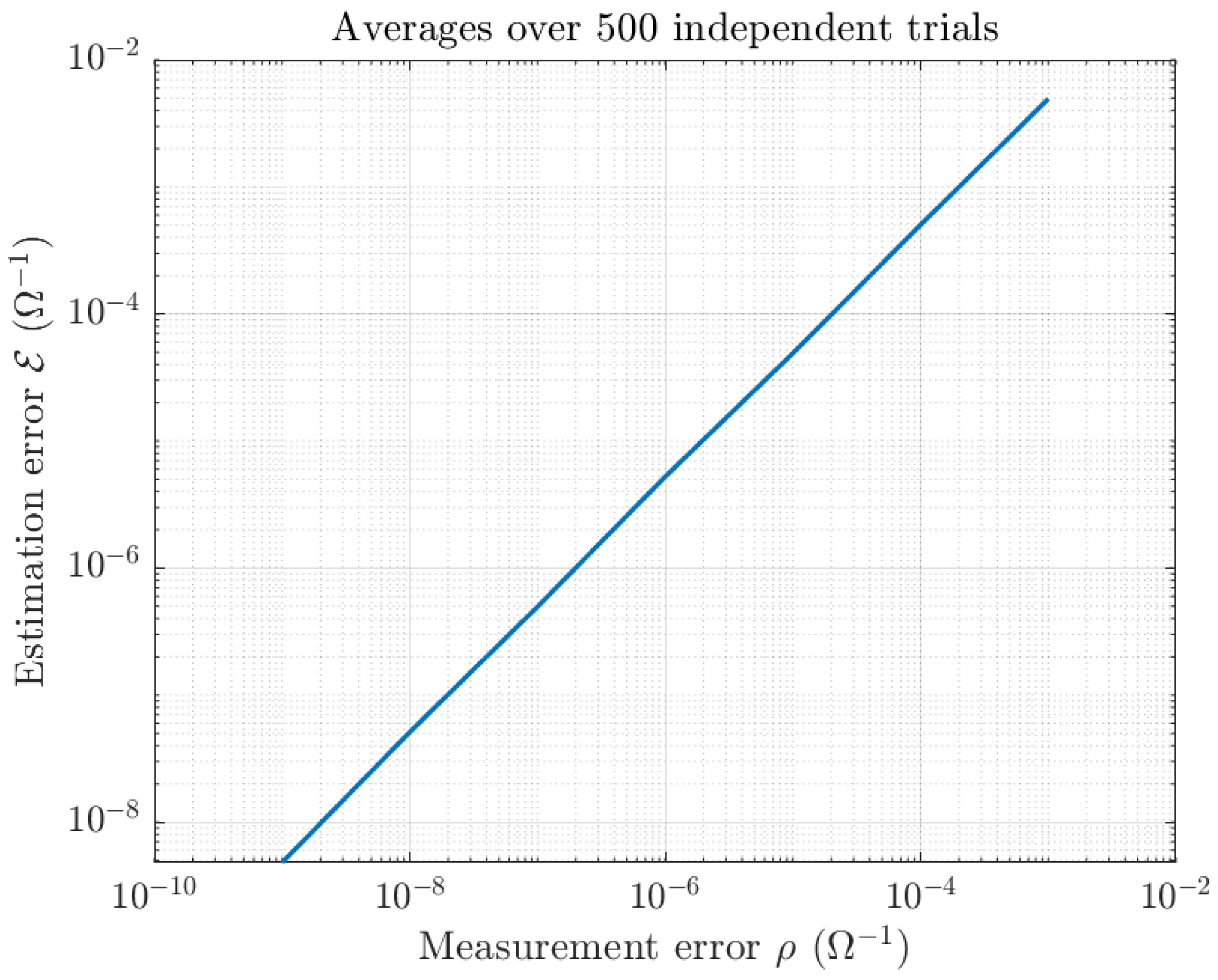
The Figure 3 shows the result of adding random errors to the data-pairs and evaluating the resulting mismatch in the estimated two-port model.
The curve represents the average result obtained over 500 independent trials.
The displayed curve shows a quasi-linear dependence between the estimation error and the measurement error levels in a logarithmic scale, which corresponds to an exponential dependence of the kind E ρ k . In other terms, as is readily appreciated, even modest measurement error levels result in a noticeable mismatch in the model estimation.
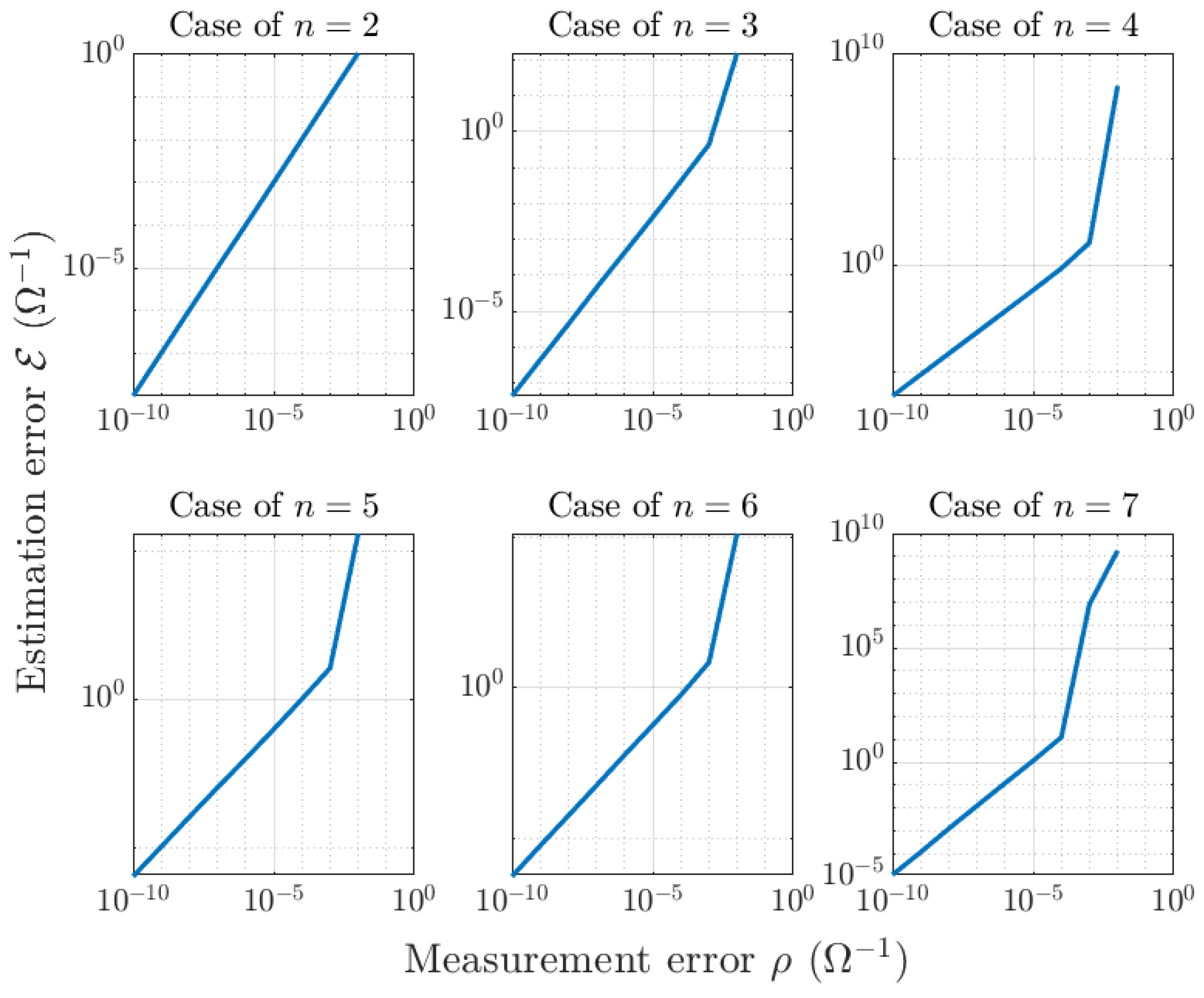
The following tests of this series concern the case that the size n ranges from 2 to 7. The obtained results are summarized in the Figure 4.
Apparently, as the size of the admittance matrices that are to be estimated grows, the effect of measurement noise on the quality of the estimations also increases.
A major concern that emerges from these simulated experiments is that the measurement errors is amplified by the estimation algorithm; therefore, the results of identification process are no longer reliable.

4.2. Testing the Iterative Algorithm: Dataset and Initial Guess

The data-pairs ( Y S ( k ) , Y M ( k ) ) were constructed by choosing an admittance matrix Y ¯ S + ( 2 n ) + j S ( 2 n ) and generating the known-loads Y S ( k ) S + ( n ) + j S ( n ) and the corresponding measurements Y M ( k ) S + ( n ) + j S ( n ) by means of the relationship (22). The size n 1 was selected beforehand and determines the complexity of the identification problem. The synthetic measurements were then corrupted by noise.
To be more specific, let us define the operator σ : R n × n S ( n ) as σ ( M ) : = 1 2 ( M + M ) , which takes any square matrix and turns it into a symmetric matrix. The actual 2 n -port model admittance matrix was randomly generated by means of the relationship
Y ¯ : = Exp ( σ ( R 1 ) ) + j σ ( R 2 ) ,
where R 1 , R 2 are two 2 n × 2 n real-valued random matrices whose entries are drawn from a zero-mean Gaussian distribution. The standard deviation of the entries of the matrix R 1 was set to 0.9 , while the standard deviation of the entries of the matrix R 2 was set to 1.5 .
Likewise, the K error-free known-loads were randomly generated by the rule
Y ¯ S ( k ) : = Exp ( σ ( R 3 ( k ) ) ) + j σ ( R 4 ( k ) ) ,
where R 3 ( k ) , R 4 ( k ) , for k = 1 , 2 , , , K , are n × n real-valued random matrices whose entries are drawn from a zero-mean Gaussian distribution. The standard deviation of the entries of the matrices R 3 was set to 0.3 , while the standard deviation of the entries of the matrices R 4 was set to 1.5 .
The synthetic error-free measurements were then generated by the relation
Y ¯ M ( k ) = Y ¯ EE Y ¯ EI ( Y ¯ S ( k ) + Y ¯ II ) 1 Y ¯ EI ,
where Y ¯ EE , Y ¯ II and Y ¯ EI denote the three independent n × n blocks of the matrix Y ¯ .
Both the error-free synthetic known-loads and the synthetic measurements were corrupted by measurement errors by the following relationships, which preserve the positive-definiteness of the conductance components of the admittances:
Y S ( k ) : = Exp ( Log ( Re { Y ¯ S ( k ) } ) + σ ( R 5 ( k ) ) ) + j ( Im { Y ¯ S ( k ) } + σ ( R 6 ( k ) ) ) , Y M ( k ) : = Exp ( Log ( Re { Y ¯ M ( k ) } ) + σ ( R 7 ( k ) ) ) + j ( Im { Y ¯ M ( k ) } + σ ( R 8 ( k ) ) ) ,
where R 5 ( k ) , R 6 ( k ) , R 7 ( k ) and R 8 ( k ) , for k = 1 , 2 , , , K , denote n × n real-valued random matrices whose entries are drawn from a zero-mean Gaussian distribution.
In all the following experiments, the standard deviation of the entries of the matrices R 5 , R 6 , R 7 and R 8 was set to 0.01 and the number of known-loads was set to K = 50 .
To start the iteration, it is necessary to set an initial guess. In all following numerical experiments, we set
Y 0 : = Exp ( Log ( Re { Y ¯ } ) + σ ( R 9 ) ) + j ( Im { Y ¯ } + σ ( R 10 ) ) ,
where R 9 and R 10 are 2 n × 2 n real-valued random matrices whose entries are drawn from a zero-mean Gaussian distribution with a standard deviation equal to 0.3 .
Note. The magnitude order of the entries of the matrices is not a concern, because one may always invoke the notion of normalization within a given operation range. This is a well-known notion from circuit theory that we may recall with a simple example: The admittance of a capacitor of capacitance C in Farad (F) at the frequency f in Hertz (Hz) is Y c : = 2 π j f C ; now, the admittance corresponding to a (realistic, un-normalized) pair f = 10 9 Hz and C = 10 9 F is the same corresponding to the (non-realistic, normalized) pair f = 1 Hz and C = 1 F.
In the following experiments, the halting criterion is based on a prefixed number of iterations, whose value may be desumed directly from the displayed figures.

4.3. Testing the Iterative Algorithm: Definition of Performance Figures

The entity of the measurement errors affecting the known loads as well as the equivalent external admittance is quantified by the value
β 2 : = 1 K k = 1 K Exp ( σ ( R 5 ( k ) ) ) 2 + σ ( R 6 ( k ) ) 2 + Exp ( σ ( R 7 ( k ) ) ) 2 + σ ( R 8 ( k ) ) 2 ,
which increases as the entity of the errors affecting the measures increases.
In order to quantify the performances of the devised numerical optimization algorithm, we define a global modeling error at the -th iteration as
E : = 1 K k = 1 K Y M ( k ) Y EE , + Y EI , ( Y S ( k ) + Y II , ) 1 Y EI , ,
that accounts for the total error over each data pair corresponding to a current estimation Y of the electronic chip package’s admittance matrix. This error depends on the data and may be evaluated even when the actual admittance matrix Y ¯ is unknown.
In addition, we defined a modeling error with respect to the known model Y ¯ pertaining to the real part and to the imaginary part of the variables, separately. To quantify the error in the real part of the sought admittance matrix, we need to define the notion of manifold logarithmic map as the inverse of the exponential map (48), that is   
log X S + ( 2 n ) ( Z ) : = X 1 2 Log ( X 1 2 Z X 1 2 ) X 1 2 ,
where X , Z S + ( 2 n ) and the symbol Log denotes principal matrix logarithm. On the basis of the above logarithmic map, it is possible to evaluate the distance between two symmetric, positive-definite matrices induced by the canonical metric, namely
d S + ( 2 n ) ( X , Z ) = log X S + ( 2 n ) ( Z ) , log X S + ( 2 n ) ( Z ) X 1 2 = tr ( Log 2 ( X 1 2 Z X 1 2 ) ) .
The errors in the estimation of the real part and of the imaginary part of the admittance matrix, under the assumption that no sign reversal occurs in the off-diagonal blocks, are then defined as
R : = d S + ( 2 n ) Y Re , Re { Y ¯ } , I : = Y Im Im { Y ¯ } ,
respectively, both referred to the iteration step . (In case of sign reversion, the above errors need to be replaced by R ¯ : = d S + ( 2 n ) J Y Re J , Re { Y ¯ } and I ¯ : = J Y Im J Im { Y ¯ } , where the matrix J was defined in the Section 2.7). Note that these errors may be evaluated only during a test phase, where the actual value of the model Y ¯ is known in advance.

4.4. Numerical Test on the Iterative Algorithm with n = 1

This special case, where the unknowns Y EE , Y EI and Y II as well as the known data-pairs ( Y S ( k ) , Y M ( k ) ) , for k = 1 , 2 , , K , are complex-valued scalars, has been treated in detail in the examples discussed throughout the present paper. In the present section, a numerical test regarding the identification of a two-port is described and the obtained results are discussed.
We can recall that a symmetric positive-definite matrix has precisely one symmetric positive-definite square root [32]. In S + ( 2 ) , a matrix square root may be written explicitly. In the present context:
( Y Re ) 1 2 : = 1 Y EE Re + Y II Re + 2 det ( Y Re ) Y EE Re + det ( Y Re ) Y EI Re Y EI Re Y II Re + det ( Y Re ) ,
with det ( Y Re ) = Y EE Re Y II Re ( Y EI Re ) 2 . Let us recall from Section 3 that Y EE Re > 0 , Y II Re > 0 and det ( Y Re ) > 0 , therefore the above matrix-square-root is well-defined.
In addition, we recall that the matrix exponential of a 2 × 2 real-valued symmetric matrix may be written explicitly. (In general, the exponential of a n × n matrix S may be written in closed form as a matrix polynomial in S of degree at most n 1 , whose coefficients are functions of the eigenvalues of S. The structure of the coefficients of the polynomial depends on the size n and needs to be written down explicitly once the size n is determined). An explicit formula for the matrix exponential of a 2 × 2 symmetric matrix S is
Exp ( S ) = e λ ( ( 1 λ ) I 2 + S )   if   μ = λ , μ e λ λ e μ μ λ I 2 + e μ e λ μ λ S   if   μ λ ,
where λ , μ R denote the eigenvalues of the matrix S, as explained, for instance, in [33].
The devised manifold-calculus-based optimization algorithm for the case that n = 1 is summarized as follows:
Y + 1 Re = ( Y Re ) 1 2 Exp η Re ( Y Re ) 1 2 Re { M } ( Y Re ) 1 2 ( Y Re ) 1 2 , Y + 1 Im = Y Im η Im Im { M } ,
where the involved matrices read, specifically:
M : = k = 1 K ( Y M ( k ) Y EE , ) ( Y S ( k ) + Y II , ) + Y EI , 2 Y S ( k ) + Y II , ( Y M ( k ) Y EE , ) ( Y S ( k ) + Y II , ) Y EI , * + Y EI , | Y EI , | 2 | Y S ( k ) + Y II , | 2 ( Y M ( k ) Y EE , ) ( Y S ( k ) + Y II , ) Y EI , * + Y EI , | Y EI , | 2 | Y S ( k ) + Y II , | 2 ( Y M ( k ) Y EE , ) ( Y S ( k ) + Y II , ) Y EI , 2 * + | Y EI , | 4 ( Y S ( k ) + Y II , ) * | Y S ( k ) + Y II , | 2 , Y EE , = Y EE , Re + j Y EE , Im , Y EI , = Y EI , Re + j Y EI , Im , Y II , = Y II , Re + j Y II , Im , Y Re = Y EE , Re Y EI , Re Y EI , Re Y II , Re , Y Im = Y EE , Im Y EI , Im Y EI , Im Y II , Im .
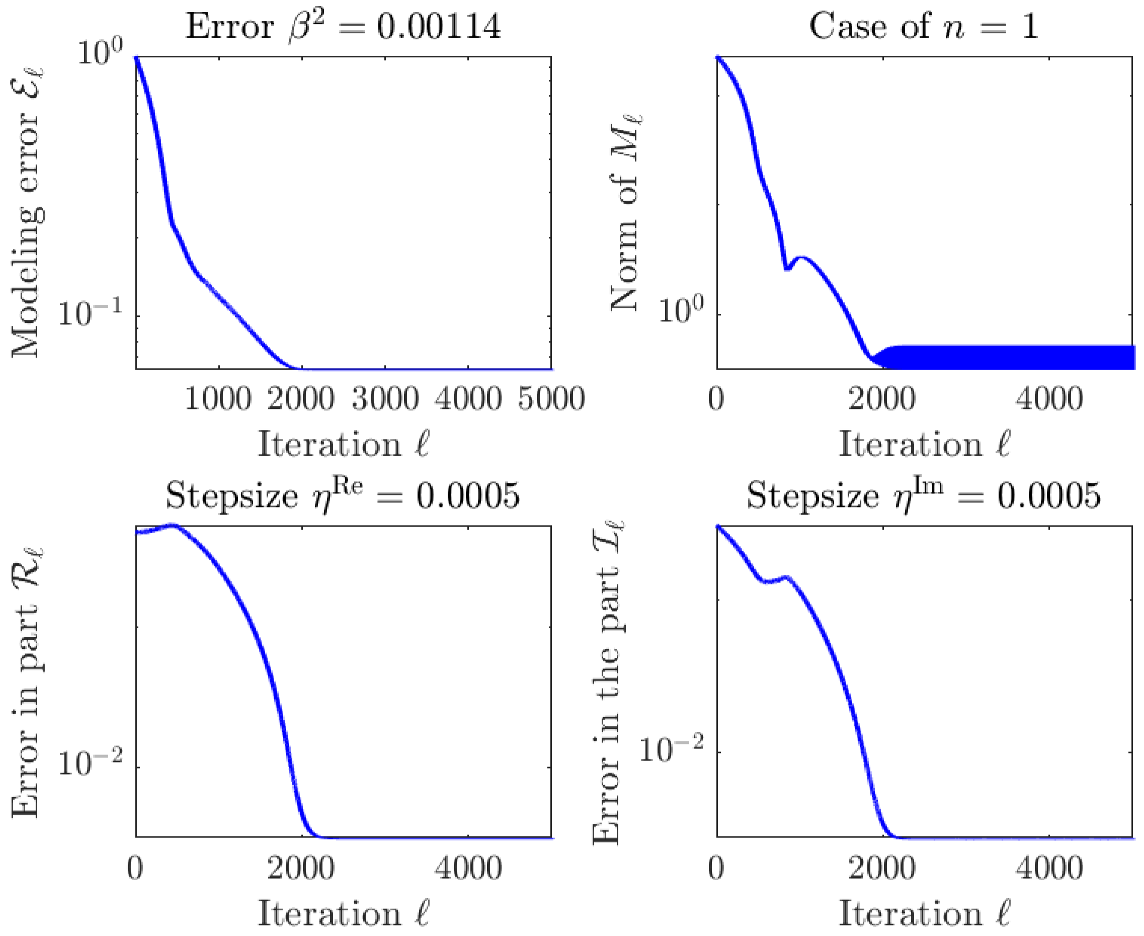
The results of a numerical experiment are illustrated in the Figure 5. As may be readily appreciated from the curves shown in this figure, the modeling errors concerning the real and the imaginary part of the variable matrix Y steadily decrease and remain stable after convergence is achieved, which signifies that the numerical optimization algorithm is numerically stable.
The (randomly generated) initial guess of the admittance matrix to start the algorithmic iteration reads
Y 0 = 1.4363 0.4517 j 0.0047 + 2.5924 j 0.0047 + 2.5924 j 0.2886 + 1.2669 j Ω 1 .
The actual simulated admittance matrix of the two-port under modeling, in this experiment, was
Y ¯ = 1.0246 0.5079 j 0.2225 + 2.9846 j 0.2225 + 2.9846 j 0.3483 + 1.3017 j Ω 1 ,
while the estimated admittance matrix of the two-port through the devised algorithm equals
Y = 1.0302 0.4570 j 0.2031 + 2.9799 j 0.2031 + 2.9799 j 0.3449 + 1.2924 j Ω 1 .
For this experiment, we report the whole dataset used in the numerical simulation in Table 1.
The relative global estimation error (namely, the final error compared to the initial error) equals 6.2 % . The absolute global modeling error equals 0.0691 Ω 1 . Note that the order of magnitude of the absolute global estimation error is the same as the standard deviation of the measurement error.
A de-embedding of a DUT from the package/connector was simulated. The actual simulated admittance of the DUT was Y ¯ D = 1.2863 0.5494 j Ω 1 , while the estimated admittance of the DUT calculated through the relation explained in Section 2.6 was Y D = 1.2820 0.5488 j Ω 1 .

4.5. Numerical Tests on the Iterative Algorithm with n > 1

In the full-matrix case, namely, when the integer n is arbitrary, the unknowns Y EE , Y EI and Y II , as well as the known data-pairs ( Y S ( k ) , Y M ( k ) ) , for k = 1 , 2 , , K , are complex-valued n × n matrices.
In the present section, progressively more complicated estimation problems will be considered, with the integer n ranging from 2 to 6. The obtained results will be illustrated in terms of convergence curves and through full matrices, as long as their size fits the page width. In particular, since the real part and the imaginary part of the unknown admittance matrix Y are updated according to mathematical rules of different conception, namely, a rule based on geodesic stepping and a rule based on standard Euler stepping, the figures will separately survey the speed of convergence of the real and imaginary part of package admittance variable-matrix Y.
We specify that, in the Matlab ® codes, the matrix exponential is computed through the expm function, while the matrix-square-root is computed by the sqrtm function. We notice that, for both matrix-functions, there are alternative calculation rules, which are either more efficient or more precise. However, in the present paper, numerical complexity is of no concern since model identification is supposed to be performed offline. In general, in the context of numerical optimization, the precision of single steps is also of no concern since all that matters is the precision of the achieved solution.
The Riemannian-gradient-based geodesic-stepping optimization algorithm in the full matrix case is expressed again as in (76), where the necessary working quantities are as follows:
M : = k = 1 K Λ ( k ) Λ ( k ) Y EI , * ( Y S ( k ) + Y II , ) * ( Λ ( k ) Y EI , * ( Y S ( k ) + Y II , ) * ) ( Y S ( k ) + Y II , ) * Y EI , Λ ( k ) Y EI , * ( Y S ( k ) + Y II , ) * , Λ ( k ) : = Y M ( k ) Y EE , + Y EI , ( Y S ( k ) + Y II , ) 1 Y EI , , Y EE , = Y EE , Re + j Y EE , Im , Y EI , = Y EI , Re + j Y EI , Im , Y II , = Y II , Re + j Y II , Im , Y Re = Y EE , Re Y EI , Re ( Y EI , Re ) Y II , Re , Y Im = Y EE , Im Y EI , Im ( Y EI , Im ) Y II , Im .
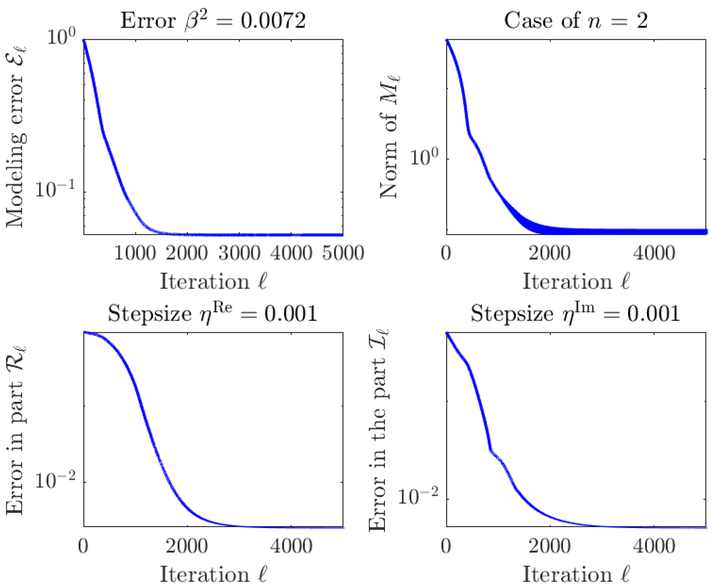
The results of a numerical experiments performed with n = 2 are illustrated in the Figure 6.
The (randomly generated) initial guess reads
Y 0 = 1.6729 + 2.2931 j 1.2798 + 1.2160 j 0.6483 + 1.7859 j 1.1588 + 1.8031 j 1.2798 + 1.2160 j 2.8347 1.3807 j 0.2173 1.9424 j 2.9445 1.6019 j 0.6483 + 1.7859 j 0.2173 1.9424 j 1.1749 0.1453 j 0.1298 0.8123 j 1.1588 + 1.8031 j 2.9445 1.6019 j 0.1298 0.8123 j 4.1929 0.3826 j Ω 1 .
The actual simulated admittance matrix of the multiport under modeling is
Y ¯ = 0.8843 + 2.4645 j 0.6441 + 1.6827 j 0.4110 + 1.8928 j 0.4964 + 1.8550 j 0.6441 + 1.6827 j 1.2938 1.1192 j 0.3009 1.3390 j 1.0067 1.6688 j 0.4110 + 1.8928 j 0.3009 1.3390 j 1.4822 0.0129 j 0.0093 0.8279 j 0.4964 + 1.8550 j 1.0067 1.6688 j 0.0093 0.8279 j 1.9016 0.3350 j Ω 1 ,
and the estimated admittance matrix of the multiport through the devised algorithm equals
Y = 0.9117 + 2.4795 j 0.6244 + 1.6635 j 0.4083 + 1.8660 j 0.5080 + 1.8279 j 0.6244 + 1.6635 j 1.3006 1.0922 j 0.2982 1.3230 j 0.9749 1.6435 j 0.4083 + 1.8660 j 0.2982 1.3230 j 1.4689 + 0.0020 j 0.0106 0.8439 j 0.5080 + 1.8279 j 0.9749 1.6435 j 0.0106 0.8439 j 1.8468 0.3475 j Ω 1 .
The relative global estimation error (namely, the final error compared to the initial error) equals 2.8 % . The absolute global modeling error equals 0.0465 Ω 1 . Note that the order of magnitude of the absolute global estimation error is the same as the measurement error standard deviation.
A simulated de-embedding of a device-under-testing from the electronic chip package was operated. The actual simulated admittance matrix of the DUT reads
Y ¯ D = 1.0315 0.2443 j 0.0472 1.2728 j 0.0472 1.2728 j 1.1561 0.9266 j Ω 1 ,
while the estimated admittance matrix of the device under testing reads
Y D = 1.0160 0.2392 j 0.0457 1.2658 j 0.0457 1.2658 j 1.1171 0.9249 j Ω 1 .
The obtained result is in good agreement with the actual admittance matrix, and the error in the estimation is of the same order of the simulated measurement errors.
The results of a numerical experiment obtained with n = 3 are illustrated in the Figure 7.
In this experiment, the relative global estimation error after optimization is 34.9 % , while the absolute global modeling error equals 0.0756 Ω 1 . Nevertheless, the order of magnitude of the absolute global estimation error is the same of the measurement error standard deviation.
A de-embedding was simulated through a numerical experiment. The actual simulated admittance matrix of the DUT reads
Y ¯ D = 1.9676 0.6691 j 2.7321 0.7434 j 4.6995 0.6069 j 2.7321 0.7434 j 4.5285 0.5506 j 5.7589 + 1.3203 j 4.6995 0.6069 j 5.7589 + 1.3203 j 12.7101 0.5425 j Ω 1 ,
while the admittance matrix of the simulated DUT, estimated through the external identification algorithm, reads
Y D = 1.9925 0.6086 j 2.8704 0.8759 j 4.9302 0.7001 j 2.8704 0.8759 j 4.8933 0.4124 j 6.2649 + 1.3452 j 4.9302 0.7001 j 6.2649 + 1.3452 j 13.4297 0.7506 j Ω 1 .
Certainly, the whole estimation/de-embedding process suffers because of an increasing problem size, although the obtained result appears to be in good agreement with the expected numerical values given the presence of measurement errors.
The outcomes of a further numerical experiment obtained by setting n = 4 are illustrated in the Figure 8. Even in this experiment, the convergence to an optimal solution looks steady and stable.
The relative global estimation error after convergence equals 2.5 % and the absolute global modeling error equals 0.0866 Ω 1 .
Still for the experiment with n = 4 , Table 2 shows the eigenvalues of the actual conductance matrix Re { Y ¯ } , as well as the eigenvalues of the estimated conductance matrix Re { Y } for comparison purposes.
The eigenvalues of the estimated conductance matrix are in excellent agreement with the eigenvalues of the actual conductance matrix, which is a further indicator of the quality of the solution and the robustness of the estimation algorithm against measurement errors.
Even in this instance, a simulated de-embedding was operated. The actual simulated admittance matrix of the device under testing reads
Y ¯ D = 0.6695 + 0.0907 j 0.3380 + 1.2023 j 1.0583 0.5594 j 0.8518 + 1.7162 j 0.3380 + 1.2023 j 0.4424 2.0950 j 0.2798 0.1147 j 0.0501 0.6896 j 1.0583 0.5594 j 0.2798 0.1147 j 2.5576 + 1.7276 j 2.3586 + 1.3821 j 0.8518 + 1.7162 j 0.0501 0.6896 j 2.3586 + 1.3821 j 2.4361 + 0.6677 j Ω 1 ,
while the estimated admittance matrix of the numerically simulated device reads
Y D = 0.6556 + 0.1137 j 0.3624 + 1.1810 j 1.0772 0.5541 j 0.8800 + 1.7338 j 0.3624 + 1.1810 j 0.4311 2.0919 j 0.3050 0.1560 j 0.0513 0.6921 j 1.0772 0.5541 j 0.3050 0.1560 j 2.5652 + 1.7796 j 2.3477 + 1.4369 j 0.8800 + 1.7338 j 0.0513 0.6921 j 2.3477 + 1.4369 j 2.4412 + 0.7626 j Ω 1 .
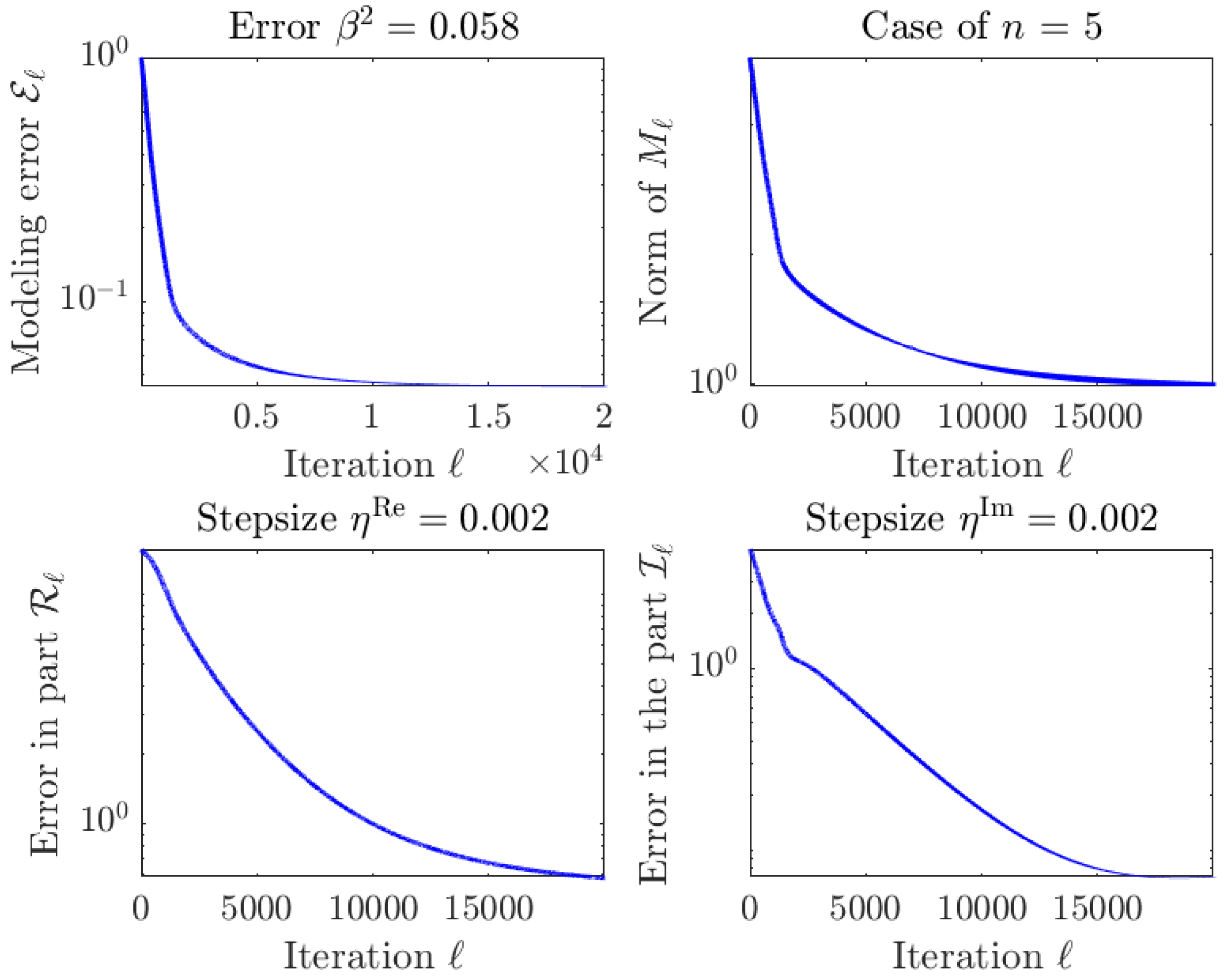
The results of a further numerical experiment pertaining to a number of internal/external ports of n = 5 are illustrated in the Figure 9. From this figure, the total measurement error affecting the data is shown to increase with the size of the problem and, at the same time, the convergence of the optimization algorithm becomes slower, although it remains steady.
In this experiment, the relative global modeling error after iteration attests to 4.5 % , with an absolute global modeling error of 0.166 . The eigenvalue comparison shown in the Table 3 confirms that the algorithm can recover the eigenstructure of the conductance part with good precision.
A result of simulated embedding confirms the above conclusions: When the actual admittance matrix of the DUT reads
Y ¯ D = 2.7822 + 1.3378 j 1.7279 + 0.5760 j 0.2772 + 2.6109 j 1.9181 1.7692 j 0.7222 1.5057 j 1.7279 + 0.5760 j 4.6236 + 1.1261 j 2.1491 + 1.9037 j 2.3820 + 1.0605 j 0.1982 3.3572 j 0.2772 + 2.6109 j 2.1491 + 1.9037 j 1.1591 + 0.9735 j 0.7353 + 0.4465 j 0.0134 + 0.8203 j 1.9181 1.7692 j 2.3820 + 1.0605 j 0.7353 + 0.4465 j 2.3560 + 0.2259 j 0.0595 + 0.3476 j 0.7222 1.5057 j 0.1982 3.3572 j 0.0134 + 0.8203 j 0.0595 + 0.3476 j 0.5141 + 3.6769 j Ω 1 ,
the corresponding admittance matrix estimated after completing the identification of the multiport reads
Y D = 2.7721 + 1.3399 j 1.7378 + 0.5455 j 0.3065 + 2.6136 j 1.9616 1.7040 j 0.6951 1.4498 j 1.6933 + 0.5518 j 4.5485 + 1.1475 j 2.1786 + 1.9144 j 2.2832 + 1.2198 j 0.1221 3.3751 j 0.2821 + 2.6223 j 2.2023 + 1.9042 j 1.1621 + 0.9535 j 0.8159 + 0.4030 j 0.0596 + 0.9525 j 1.9228 1.7165 j 2.2391 + 1.2273 j 0.7695 + 0.3980 j 2.1058 0.1718 j 0.1474 + 0.1153 j 0.6982 1.4936 j 0.0967 3.3486 j 0.0486 + 0.9215 j 0.1217 + 0.1320 j 0.4447 + 3.5238 j Ω 1 .
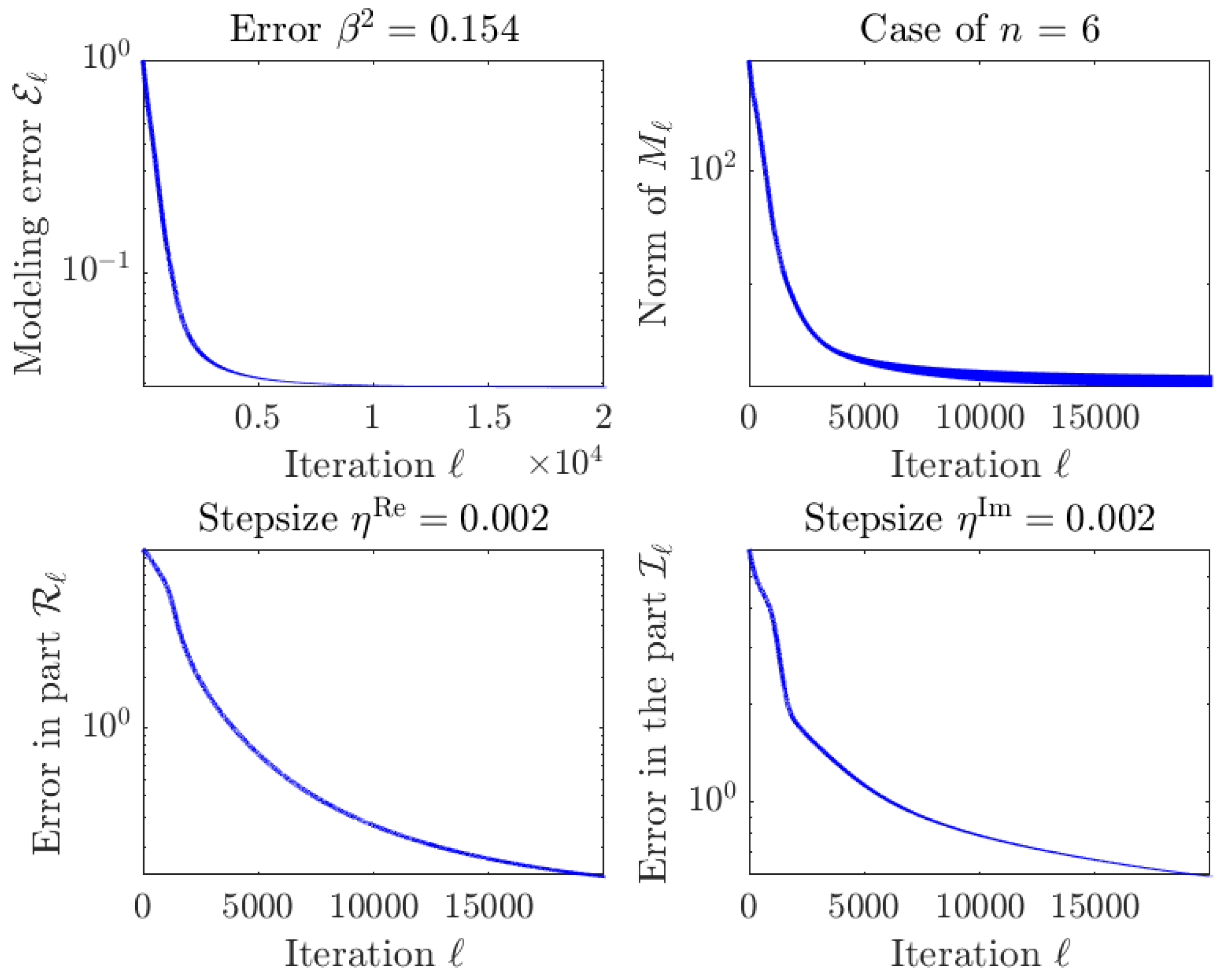
As a last test, a numerical experiment was carried on with n = 6 , whose results are illustrated in the Figure 10. Even in this numerical experiment, the achieved convergence is steady, although slower than in the previous experiments due to the increased size of the optimization problem: note that the size of the optimization problem to be solved grows twice as fast as the number of internal/external ports n.
From Figure 10, it can be seen that the number K of iteration was chosen to be excessively low, which essentially resulted in a premature halting of the optimization procedure. A larger number of iterations would have led to a more precise estimation of the conductance matrix of the simulated electronic chip package/connector.
The Table 4 shows the eigenvalues of the actual conductance matrix Re { Y ¯ } , as well as the eigenvalues of the estimated conductance matrix Re { Y } for comparison. In this case, since the number of internal/external ports equals 6, the number of estimated eigenvalues equals 12. Nevertheless, the values in the table show excellent agreement, even though the iteration halted prematurely.

5. Conclusions

The present paper dealt with a circuit-theoretic problem, framed as the external identification of a reciprocal, special passive, 2 n -port network under measurement uncertainties. The application is the de-embedding of a device under testing from an electronic chip package/connector.
An admittance-matrix representation was chosen to model the multiport equivalent circuit and the condition that the circuit under modeling is ‘reciprocal special passive’ results in the assumption that the real part of the admittance matrix is symmetric, positive-definite.
The identification problem was cast as a matrix optimization problem over the matrix manifold S + ( 2 n ) × S ( 2 n ) , based on a least-squares criterion function. This criterion was specifically crafted to cope with over-determinacy due to the cardinality of data-pairs exceeding the number of degrees of freedom of the problem.
The present paper proposed and numerically evaluated an iterative algorithm to carry on such optimization based on the Riemannian-gradient steepest descent method. A number of numerical results confirmed that the proposed method is effective as long as reasonable measurement error levels and problem sizes are dealt with.
We are currently studying an alternative approach based on a ‘matrix polynomial’ formulation of the loss function f ˜ , in contrast to the present formulation, which may be referred to as ‘rational’. The novel approach under investigation is based, however, on more restrictive hypotheses regarding the structure of the sought admittance matrix Y, and will thus be of a less general scope than the one presented in this paper.

Author Contributions

Conceptualization, S.F.; methodology, S.F. and J.W.; software, S.F.; formal analysis, S.F. and J.W.; writing—original draft preparation, S.F. and J.W.; writing—review and editing, S.F. and J.W. All authors have read and agreed to the published version of the manuscript.

Funding

Part of this research was carried out while the authors were on leave at the National Center for Theoretical Sciences (NCTS, National Taiwan University, Taipei), funded by a “Research in Pairs” program, during August 2016. In addition, the author JW was partially funded by the General Project of Science and Technology Plan of Beijing Municipal Education Commission (Grant No. KM202010037003).

Data Availability Statement

Some data from the experiments were created randomly by computer code and are no longer available.

Acknowledgments

The authors worked jointly on the theoretical development and on the computer codes to implement the devised algorithm. The computer codes were then validated by a number of students over the last six years, including X. Han, F. Marcucci, R. Saraceni and J. Sgariglia, whose contribution is gratefully acknowledged.

Conflicts of Interest

The authors declare no conflict of interest.

References

  1. Mimani, A.; Munjal, M.L. Acoustical analysis of a general network of multi-port elements—An impedance matrix approach. Int. J. Acoust. Vib. 2012, 17, 23–46. [Google Scholar]
  2. Kim, N.; Allen, J.B. Allen Two-port network analysis and modeling of a balanced armature receiver. Hear. Res. 2013, 301, 156–167. [Google Scholar] [CrossRef] [PubMed]
  3. Snakowska, A.; Jurkiewicz, J. A new approach to the theory of acoustic multi-port networks with multimode wave and its application to muffler analysis. J. Sound Vib. 2021, 490, 115722. [Google Scholar] [CrossRef]
  4. Lee, H.; Lee, C.; Jang, G.; Kwon, S.-h. Harmonic analysis of the Korean high-speed railway using the eight-port representation model. IEEE Trans. Power Deliv. 2006, 21, 979–986. [Google Scholar] [CrossRef]
  5. Frasch, H.F.; Kresh, J.Y.; Noordergraaf, A. Two-port analysis of microcirculation: An extension of windkessel. Am. J. Physiol. 1996, 270, 376–385. [Google Scholar] [CrossRef]
  6. Manhartsgruber, B. Identification of the input-output behavior of hydraulic two-port networks. In Proceedings of the ASME 2009 Dynamic Systems and Control Conference, Hollywood, CA, USA, 12–14 October 2009; Volume 2, pp. 29–35. [Google Scholar]
  7. Farina, M.; Morini, A.; Rozzi, T. A calibration approach for the segmentation and analysis of microwave circuits. IEEE Trans. Microw. Theory Technol. 2007, 55, 2124–2134. [Google Scholar] [CrossRef]
  8. Mikulecky, D.C. A network thermodynamic two-port element to represent the coupled flow of salt and current. Improved alternative for the equivalent circuit. Biophys. J. 1979, 25, 323–340. [Google Scholar] [CrossRef] [PubMed] [Green Version]
  9. Bonnin, M.; Traversa, F.L.; Bonani, F. A cascaded two-port network model for the analysis of harmonic chain-based energy harvesters. In Proceedings of the 2021 IEEE International Conference on Environment and Electrical Engineering and 2021 IEEE Industrial and Commercial Power Systems Europe (EEEIC/I&CPS Europe), Bari, Italy, 7–10 September 2021; pp. 1–6. [Google Scholar] [CrossRef]
  10. Chung, E.; Ha, J.-I.; Bastami, A.A.; Perreault, D.J. Impedance compressing matching network based on two-port network analysis for wireless power transfer system. IEEE J. Emerg. Sel. Top. Ind. Electron. 2022, 3, 432–442. [Google Scholar] [CrossRef]
  11. Monti, G.; Mongiardo, M.; Minnaert, B.; Costanzo, A.; Tarricone, L. Optimal terminations for a single-input multiple-output resonant inductive WPT link. Energies 2020, 13, 5157. [Google Scholar] [CrossRef]
  12. Paul, R.J.A. Two-Port Network Representations of D. C. Electro-Mechanical Transducers; Note No. 121; The College of Aeronautics, Cranfield University: Cranfield, UK, 1962; Available online: https://dspace.lib.cranfield.ac.uk/handle/1826/12076 (accessed on 16 September 2022).
  13. De Gersem, H.; Srinivasan, V.; Muehle, C. Nonlinear three-port magnetic-circuit elements for simulating bending magnets. COMPEL-Int. J. Comput. Math. Electr. Electron. Eng. 2018, 37, 266–279. [Google Scholar] [CrossRef]
  14. Alazard, D.; Perez-Gonzalez, J.-A.; Loquen, T.; Cumer, C. Two-input two-output port model for mechanical systems. In Proceedings of the Scitech 2015—53rd AIAA Aerospace Sciences Meeting, Kissimmee, FL, USA, 5–9 January 2015; Available online: http://oatao.univ-toulouse.fr/13642/1/Alazard_13642.pdf (accessed on 25 September 2016).
  15. Duman, T.; Marti, S.; Moonem, M.A.; Kader, A.A.R.A.; Krishnaswami, H. A modular multilevel converter with power mismatch control for grid-connected photovoltaic systems. Energies 2017, 10, 698. [Google Scholar] [CrossRef] [Green Version]
  16. Pu, B.; Kim, J.; Nah, W. A de-embedding technique of a three-port network with two ports coupled. J. Electromagn. Eng. Sci. 2015, 15, 258–265. [Google Scholar] [CrossRef] [Green Version]
  17. Ballicchia, M.; Farina, M.; Morini, A.; Turchetti, C.; Orcioni, S. A methodology for RF modeling of packages with external pin measurements. Int. J. Microw.-Comput.-Aided Eng. 2014, 24, 623–634. [Google Scholar] [CrossRef]
  18. Schaft, A.v.; Jeltsema, D. Port-Hamiltonian systems: An introductory overview. Found. Trends Syst. Control 2014, 1, 173–378. [Google Scholar] [CrossRef]
  19. Vlach, J. Linear Circuit Theory: Matrices in Computer Applications; Apple Academic Press: Lansing, MI, USA, 2021. [Google Scholar]
  20. Kokalari, I.; Karaja, T.; Guerrisi, M. Review on lumped parameter method for modeling the blood flow in systemic arteries. J. Biomed. Sci. Eng. 2013, 6, 92–99. [Google Scholar] [CrossRef] [Green Version]
  21. Dunsmore, J.P. Handbook of Microwave Component Measurements: With Advanced VNA Techniques; Wiley: New York, NY, USA, 2012. [Google Scholar]
  22. Horn, R.A.; Johnson, C.R. Matrix Analysis; Cambridge University Press: Cambridge, UK, 1985. [Google Scholar]
  23. Boyd, S.; Chua, L.O. On the passivity criterion for LTI n-port. Circuit Theory Appl. 1982, 10, 323–333. [Google Scholar] [CrossRef]
  24. Silvester, J.R. Determinants of block matrices. Math. Gaz. 2000, 84, 460–467. [Google Scholar] [CrossRef] [Green Version]
  25. Meyer, C.D. Matrix Analysis and Applied Linear Algebra, Chapter 7.6: Positive Definite Matrices; Society for Industrial and Applied Mathematics: Philadelphia, PA, USA, 2000. [Google Scholar]
  26. Marcus, M.; Minc, H. A Survey of Matrix Theory and Matrix Inequalities; Dover Publications Inc.: Mineola, NY, USA, 1992. [Google Scholar]
  27. Nash, S.G.; Sofer, A. Linear and Nonlinear Programming; McGraw-Hill Science/Engineering/Math: New York, NY, USA, 1995. [Google Scholar]
  28. Sun, H.; Zhang, Z.; Peng, L.; Duan, X. An Elementary Introduction to Information Geometry; Science Press: Beijing, China, 2016. (In Chinese) [Google Scholar]
  29. Fiori, S. Manifold calculus in system theory and control—Fundamentals and first-order systems. Symmetry 2021, 13, 2092. [Google Scholar] [CrossRef]
  30. Fiori, S. Manifold calculus in system theory and control—Second order structures and systems. Symmetry 2022, 16, 1144. [Google Scholar] [CrossRef]
  31. Higham, N.J. Functions of Matrices: Theory and Computation; Society for Industrial and Applied Mathematics (SIAM): Philadelphia, PA, USA, 2008; ISBN 978-0-898716-46-7. [Google Scholar]
  32. Levinger, B.W. The square root of a 2×2 matrix. Math. Mag. 1980, 53, 222–224. [Google Scholar] [CrossRef]
  33. Bernstein, D.S.; So, W. Some explicit formulas for the matrix exponential. IEEE Trans. Autom. Control 1993, 38, 1228–1232. [Google Scholar] [CrossRef] [Green Version]
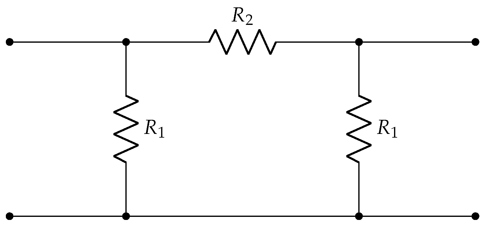
Figure 1. A simple reciprocal, energetically passive π -network, with two shunt resistors R 1 and a series resistor R 2 .
Energies 16 02585 g001
Figure 2. A resistive-capacitive standard.
Energies 16 02585 g002
Figure 3. Mismatch in an estimated two-port model resulting from random errors in the data-pairs. The horizontal axis displays the standard deviation of the measurement errors (in logarithmic scale), while the vertical axis displays the Frobenius distance between the actual and estimated two-port admittance matrix (in a logarithmic scale).
Energies 16 02585 g003
Figure 4. Mismatch in an estimated 2 n -port model resulting from random errors in the data-pairs, with n = 2 , 3 , 4 , 5 , 6 , 7 . (Graphs labelled as in Figure 3).
Energies 16 02585 g004
Figure 5. Results of a numerical experiment by the Riemannian-gradient-based geodesic-stepping optimization algorithm in the case that n = 1 . (The global modeling error is normalized to its initial value to get rid of the dependence from the random initial guess).
Energies 16 02585 g005
Figure 6. Results of a numerical experiment by the Riemannian-gradient-based geodesic-stepping optimization algorithm in the case that n = 2 .
Energies 16 02585 g006
Figure 7. Results of a numerical experiment by the Riemannian-gradient-based geodesic-stepping optimization algorithm in the case that n = 3 .
Energies 16 02585 g007
Figure 8. Results of a numerical experiment with n = 4 .
Energies 16 02585 g008
Figure 9. Results of a numerical experiment with n = 5 .
Energies 16 02585 g009
Figure 10. Results of a numerical experiment with n = 6 .
Energies 16 02585 g010
Table 1. Dataset used in the simulation and estimation error between the actual values of the equivalent admittances Y M and their estimations obtained from the estimated two-port model admittance parameters. The standards’ values were generated to simulate resistive-capacitive loads.
Admittance Y S ( Ω 1 )Admittance Y M ( Ω 1 )Error Y M Y EE + Y EI 2 / ( Y S + Y II ) ( Ω 1 )
1.1124 1.2379 j 7.0784 + 0.1597 j 0.0393 + 0.0136 j
1.1250 1.3959 j 7.0237 + 0.7732 j + 0.0678 0.0110 j
1.4534 1.5297 j 5.7792 + 0.8618 j + 0.0054 + 0.0196 j
0.9549 0.0416 j 5.0685 3.4123 j + 0.0422 0.0416 j
0.8441 1.4932 j 8.1198 + 1.7359 j + 0.0295 0.0180 j
1.4462 0.9969 j 5.9039 0.5838 j 0.0388 + 0.0077 j
0.7503 1.5660 j 8.1410 + 2.4958 j 0.2254 + 0.0143 j
1.1338 1.0174 j 6.9636 0.6809 j + 0.0086 + 0.0591 j
0.7061 0.3764 j 6.3569 3.9917 j 0.0236 0.0242 j
0.7927 1.2844 j 8.9652 + 0.4834 j + 0.1588 0.0692 j
1.9784 2.5573 j 3.6722 + 1.5033 j 0.0735 0.0394 j
1.2995 0.6294 j 5.9743 1.7234 j + 0.0652 0.0358 j
0.7838 1.4537 j 8.7559 + 1.6223 j + 0.2019 0.0687 j
0.7611 2.8225 j 3.2390 + 3.7089 j 0.0139 0.0039 j
0.7060 0.8579 j 8.7494 2.3664 j + 0.1297 + 0.0759 j
1.1209 1.5005 j 6.7809 + 1.1667 j 0.0449 0.0253 j
1.1613 1.8849 j 5.8398 + 2.2463 j + 0.0017 + 0.0081 j
0.5441 0.4434 j 6.9465 4.6594 j + 0.0362 + 0.0513 j
0.8917 0.0868 j 5.1366 3.5016 j 0.0477 + 0.0261 j
1.3726 1.0058 j 6.2036 0.5823 j + 0.0523 + 0.0244 j
1.0913 2.8658 j 3.3409 + 3.0197 j 0.0666 + 0.0292 j
0.7574 1.4048 j 8.8619 + 1.4650 j + 0.0068 + 0.0257 j
0.5844 2.1256 j 5.7117 + 4.9610 j + 0.0569 0.0317 j
0.8580 0.7926 j 7.4722 2.1901 j 0.1807 + 0.0118 j
0.7017 1.1318 j 9.4745 0.5922 j + 0.0198 + 0.0002 j
1.0018 1.8725 j 6.2774 + 2.7216 j + 0.0379 + 0.0355 j
0.8431 1.1107 j 8.3449 0.6071 j 0.1073 0.0344 j
0.7845 2.9513 j 2.9921 + 3.4805 j 0.0179 0.0425 j
0.9085 2.4065 j 4.4848 + 3.6081 j 0.0051 + 0.0240 j
1.3611 0.0412 j 4.7185 2.5225 j 0.0192 0.0563 j
0.8886 0.7737 j 7.3840 2.1390 j 0.0858 + 0.0442 j
1.2796 0.9545 j 6.3104 0.8038 j 0.0836 + 0.0234 j
1.0322 0.4597 j 6.1597 2.6596 j + 0.0403 0.0046 j
0.8424 0.7185 j 7.3588 2.5748 j 0.1054 0.0280 j
1.2344 2.0519 j 5.3342 + 2.3385 j + 0.0582 0.0129 j
1.4030 0.2168 j 5.0976 2.2274 j + 0.0903 0.0158 j
0.9254 2.3863 j 4.5861 + 3.4965 j + 0.0319 0.0343 j
0.9291 0.1008 j 5.1541 3.4381 j 0.0507 0.0268 j
1.0237 0.6549 j 6.7193 2.1823 j + 0.0438 + 0.0194 j
1.3005 2.3434 j 4.4360 + 2.4646 j 0.0753 0.0380 j
1.4438 0.3439 j 5.1942 1.9622 j + 0.0271 + 0.0116 j
1.1113 0.6057 j 6.3443 2.1407 j + 0.0279 0.0223 j
0.8153 0.0213 j 4.9847 3.7259 j 0.0278 + 0.0500 j
0.8323 0.0983 j 5.2593 3.6949 j + 0.0141 + 0.0089 j
1.6141 0.2818 j 4.8033 1.8139 j 0.0423 0.0068 j
0.8103 2.0658 j 5.9463 + 3.8327 j + 0.1176 + 0.0290 j
1.3128 0.7866 j 6.1558 1.3194 j + 0.0439 0.0422 j
0.8008 2.0980 j 5.5845 + 3.8955 j 0.1105 + 0.0154 j
1.0121 0.2593 j 5.5922 3.0262 j + 0.0083 + 0.0051 j
1.1189 0.9364 j 6.9809 1.0438 j + 0.0597 + 0.0187 j
Table 2. Eigenvalues of the estimated conductance matrix Re { Y } compared to the eigenvalues of the actual conductance matrix Re { Y ¯ } in the case n = 4 .
Eigenvalues of Re { Y ¯ } ( Ω 1 )Eigenvalues of Re { Y } ( Ω 1 )
0.06790.0777
0.13390.1323
0.31770.3189
0.36320.3649
0.97790.9513
1.52321.5382
3.00903.0088
4.70404.6554
Table 3. Eigenvalues of the estimated conductance matrix Re { Y } compared to the eigenvalues of the actual conductance matrix Re { Y ¯ } in the case n = 5 .
Eigenvalues of Re { Y ¯ } ( Ω 1 )Eigenvalues of Re { Y } ( Ω 1 )
0.01330.0081
0.14170.1394
0.19390.2003
0.31580.3333
0.84360.8209
1.14961.1470
2.32922.3371
4.03224.0452
5.53905.3469
20.111519.9327
Table 4. Eigenvalues of the estimated conductance matrix Re { Y } compared to the eigenvalues of the actual conductance matrix Re { Y ¯ } in the case n = 6 .
Eigenvalues of Re { Y ¯ } ( Ω 1 )Eigenvalues of Re { Y } ( Ω 1 )
0.08840.0884
0.13490.1348
0.24710.2644
0.36560.3906
0.53380.5278
0.56820.5858
1.57141.5986
2.26012.2647
8.44948.2849
9.816310.0289
18.833118.7491
20.898520.8803
Disclaimer/Publisher’s Note: The statements, opinions and data contained in all publications are solely those of the individual author(s) and contributor(s) and not of MDPI and/or the editor(s). MDPI and/or the editor(s) disclaim responsibility for any injury to people or property resulting from any ideas, methods, instructions or products referred to in the content.