Article

Uncertainty Analysis of CO2 Storage in Deep Saline Aquifers Using Machine Learning and Bayesian Optimization

Physical Science and Engineering Division, King Abdullah University of Science and Technology, Thuwal 23955, Saudi Arabia
*
Author to whom correspondence should be addressed.
Energies 2023, 16(4), 1684; https://doi.org/10.3390/en16041684
Submission received: 19 December 2022 / Revised: 21 January 2023 / Accepted: 30 January 2023 / Published: 8 February 2023
(This article belongs to the Special Issue Recent Advances in Reservoir Simulation)

Abstract

:
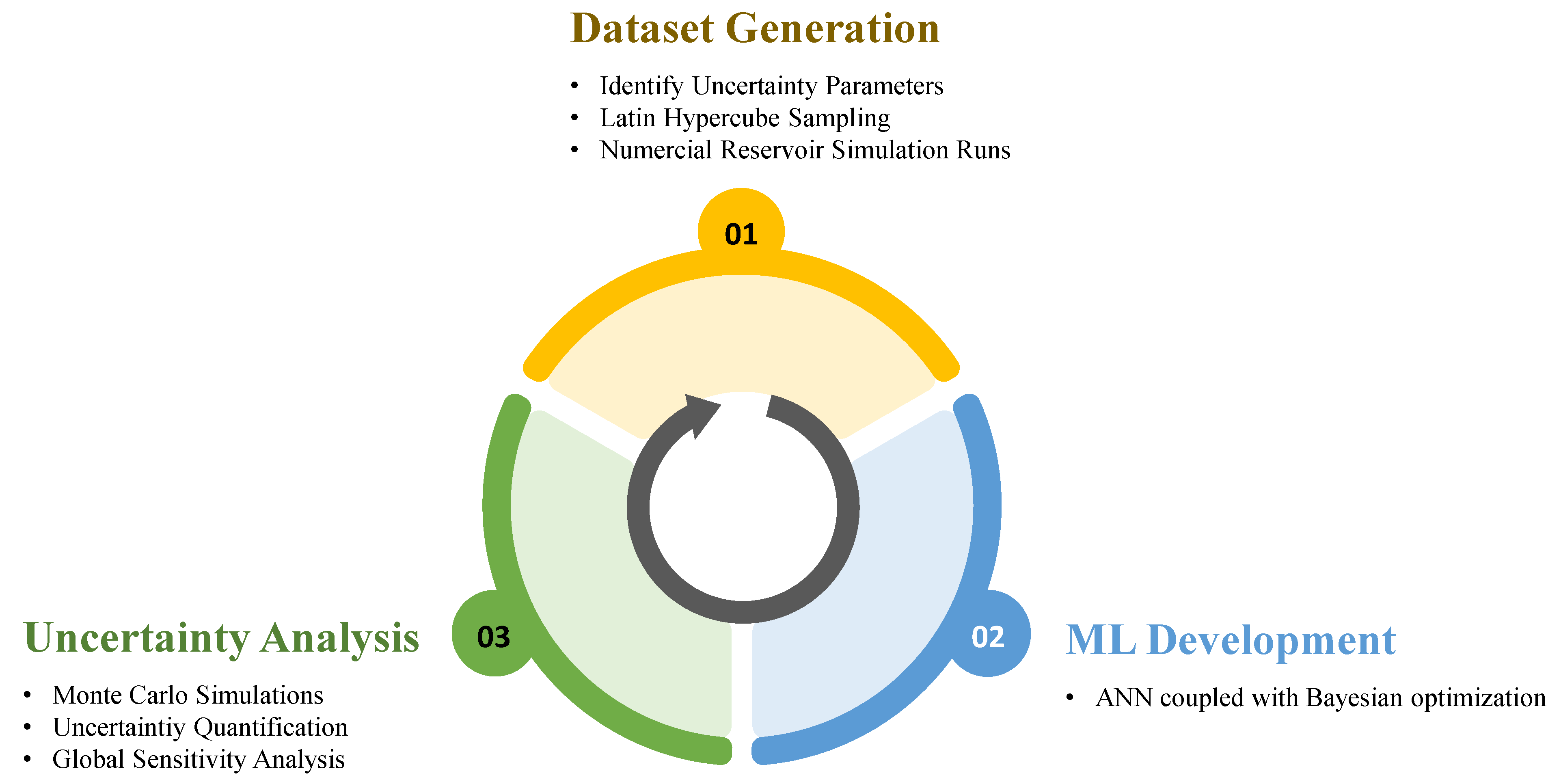
Geological CO2 sequestration (GCS) has been proposed as an effective approach to mitigate carbon emissions in the atmosphere. Uncertainty and sensitivity analysis of the fate of CO2 dynamics and storage are essential aspects of large-scale reservoir simulations. This work presents a rigorous machine learning-assisted (ML) workflow for the uncertainty and global sensitivity analysis of CO2 storage prediction in deep saline aquifers. The proposed workflow comprises three main steps: The first step concerns dataset generation, in which we identify the uncertainty parameters impacting CO2 flow and transport and then determine their corresponding ranges and distributions. The training data samples are generated by combining the Latin Hypercube Sampling (LHS) technique with high-resolution simulations. The second step involves ML model development based on a data-driven ML model, which is generated to map the nonlinear relationship between the input parameters and corresponding output interests from the previous step. We show that using Bayesian optimization significantly accelerates the tuning process of hyper-parameters, which is vastly superior to a traditional trial–error analysis. In the third step, uncertainty and global sensitivity analysis are performed using Monte Carlo simulations applied to the optimized surrogate. This step is performed to explore the time-dependent uncertainty propagation of model outputs. The key uncertainty parameters are then identified by calculating the Sobol indices based on the global sensitivity analysis. The proposed workflow is accurate and efficient and could be readily implemented in field-scale CO2 sequestration in deep saline aquifers.

1. Introduction

The current increase in the global average temperature is believed to be attributed to the high concentration of carbon dioxide (CO2) in the atmosphere, which is mostly caused by fueling the world’s economies with fossil fuels [1,2,3,4]. One practical approach to mitigating global climate change and reducing CO2 emissions is CO2 capture and storage (CCS) in the Earth’s subsurface and storing it permanently in an underground geological formation [5,6]. CO2 geological storage sites include deep saline aquifers, depleted oil and gas reservoirs, coal beds, and mineralization in reactive formations such as basalt [3,5,7,8,9,10,11,12,13]. CO2 utilization for enhanced oil recovery and sequestration into aquifers has been practiced for several decades [3], where the focus has been on deep saline aquifers due to their superior storage capacity [14]. In addition, saline aquifers are ubiquitous in many parts of the world, making them available for most existing CO2 sources [15,16].
When injecting CO2 into a deep saline aquifer formation, typically below a depth of 800 m (2600 ft), CO2 will be in its supercritical state [5]. The density of supercritical CO2 is usually less than that of resident brine, leading to upward migration of buoyant CO2 and creating a CO2 plume that spreads laterally below the impermeable cap rock. The free “mobile” CO2 plume trapped by the sealing caprock is referred to as structural trapping [7,8,17,18]. As the free CO2 phase percolates upward through the formation, a significant amount of CO2 can be entrapped by capillary forces, which is referred to as residual trapping [19,20,21]. In addition, the free CO2 phase at the CO2-brine interface will mix with the formation brine and slowly dissolve in it, leading to solubility trapping. Mineral trapping is another type of trapping mechanism in which chemical interactions between dissolved CO2 and rock minerals will occur, resulting in mineral precipitation [3,22,23]. These physical and geochemical trapping mechanisms determine the effectiveness of the storage capacity and the fate of CO2 migration [24,25,26,27,28].
Different methods have been developed to model the storage capacity, including analytical or semi-analytical studies and numerical approaches. For instance, the analytical study of quantifying leakage rates and storage used analytical models in the Laplace domain for CO2 sequestration methods [29]. In addition, a semi-analytical solution was developed to provide a simple and practical approach to evaluating the potential of CO2 leakage through abandoned wells in the subsurface storage site [30]. Moreover, several research studies used numerical-based solutions to explore storage mechanisms and assess the impact of various physical properties and constraints on storage potential [20,31,32,33]. Overall, analytical and semi-analytical solutions typically work under simplified and ideal assumptions and can be utilized for specific cases. On the other hand, numerical reservoir simulations are computationally costly and time consuming, and thus impractical for large-scale applications when multiple computations are needed, such as Monte Carlo simulations.
To address this challenge, machine learning (ML) techniques have gained significant attention in various applications, including CCS and geoscience fields, in recent years [34,35]. For instance, ML has been adapted for predicting oil production and CO2 storage in CO2-WAG injection using machine learning-assisted models [36]. Additionally, different ML methods have been utilized to investigate the potential storage and incremental oil recovery of CO2-enhanced oil recovery (CO2-EOR) projects [37,38,39]. Multiple ML models were developed to assess and predict residual and solubility trapping in deep saline aquifers [40]. These successful applications demonstrate ML’s robust capabilities to establish fast and highly accurate predictive models and offer a competitive advantage over traditional numerical simulations.
Due to the nature of the subsurface, there is always uncertainty associated with storage capacity estimates in saline aquifers. Therefore, before embarking on a large-scale CO2 geological sequestration project, an extensive assessment of the uncertainty parameters must be performed upfront to determine the long-term fate of CO2 migration and the corresponding dominant physical mechanisms. Therefore, this study proposes a rigorous workflow to perform uncertainty quantification (UQ) and global sensitivity analysis of CO2 storage capacity prediction based on a novel data-driven ML model. This study provides a robust ML-based model to predict the capacities of different trapping mechanisms in deep saline aquifers. Furthermore, it explores the uncertainty propagation using Monte Carlo simulations and conducts global sensitivity analysis by calculating the Sobol indices. Hence, to the best of our knowledge, this workflow is the first to integrate ML with Bayesian optimization, UQ, and global sensitivity analysis for CO2 storage prediction in a deep saline aquifer, corresponding to an actual field case Johansen aquifer [41]. The workflow consists of three steps: (1) perform numerical simulations to generate the required output dataset based on the input dataset designed using a specific sampling technique, (2) develop a robust predictive ML model to evaluate the trapping capacity, and (3) conduct uncertainty quantification and global sensitivity analysis using Monte Carlo simulations.
The paper is organized as follows: In Section 2, we present the governing equations of two-phase flow in porous media. The ML approach is then explained, followed by an introduction of the Johansen aquifer model. In the last part of Section 2, a detailed description of the proposed workflow is presented with a thorough explanation of each step. In Section 3, the Results and Discussion section provides the study’s outcome and justifications, followed by the main conclusions in Section 4.

2. Materials and Methods

2.1. Governing Model

In this study, we consider injecting CO2 into a saline aquifer in a supercritical phase that is less dense than the resident brine. Thus, CO2 mainly migrates via buoyancy. This work focuses primarily on structural and residual trapping mechanisms; hence, dissolution and mineral trappings are neglected. The open-source MATLAB Reservoir Simulation Toolbox (MRST) [42,43] is used to investigate CO2 flow and transport, which are governed by the conservation equation and the extended Darcy’s law, such that
( ϕ ρ α S α ) t + ( ρ α u α ) = Q α , α = CO 2 ,  
u α = k r a μ α K ( p α + ρ α g   z )
where ϕ is the porosity and t is the time; ρ α , S α , u α , Q α , k r a , μ α , and p α are the density, phase saturation, velocity, sink/source term (volumetric rate), relative permeability, viscosity, and pressure for phase α , respectively; subscription α represents the phases for CO2 and water, respectively; K is the absolute permeability tensor, g is the gravity acceleration, and z is the depth. The two-phase saturations are constrained as follows:
S C O 2 + S w = 1
We relate the two pressures via capillary pressure (denoted by pc):
p c ( S w ) = p C O 2 p w
Fluid segregation is almost instantaneous compared to the lateral movement of the CO2 plume due to the density difference between the supercritical CO2 and brine [27,44]. Therefore, a high vertical resolution is needed to capture the plume shape and resolve the vertical segregation within. Therefore, using standard 3D simulation tools for large-scale, long-term CO2 migration can be challenging and computationally expensive [8,45]. For instance, 3D simulators tend to underestimate CO2 migration velocities in simple conceptual models [45]. Therefore, in this study, we adopt a simulation approach based on the assumption of vertical equilibrium (VE), which reduces the model’s dimensionality to 2D while capturing the 3D model’s performance via the upscaled variables. The primary assumption underlying VE models is the existence of equilibrium in the vertical direction. The CO2-brine system is always segregated and in vertical equilibrium and the vertical flow constitutes a small component in the overall flow, especially for laterally extended aquifers. In fact, the strong buoyant segregation that characterizes the CO2-brine system makes VE modeling an efficient approach [46,47]. Furthermore, studies have shown how a 3D simulation gradually converges to the corresponding VE simulation as the grid resolution in the vertical direction is increased. One can find a detailed description and more information about the concept of VE-based simulation modeling and a comparison of the accuracy of VE simulation to a 3D simulation in the literature [8,46,47].
The thermodynamic properties of CO2 are calculated using the Span and Wager equation of state [48,49]. In this work, CO2 mineralization is not considered.

2.2. Machine Learning Approach

Machine learning (ML), sometimes called statistical learning, is an automated data analysis process aiming to understand the data and detect possible relationships between the data features [50]. Within ML, there are two basic approaches: supervised and unsupervised learning. Supervised learning is the learning process based on labeled input-output pairs that correlates input to output [51]. In this study, the type of learning task is supervised learning, as the input data are labeled, and the output is supplied by the numerical simulator.
Among the various machine learning techniques, the decision to select which technique would ultimately provide the most accurate prediction is a challenging task. Generally, some sophisticated ML models, such as Artificial Neural Networks (ANN), can offer satisfactory results but require extensive effort to construct and fine-tune the algorithm. Nevertheless, the same problem can be handled by a simpler machine learning technique and still provide an acceptable result. Therefore, a thorough understanding of the problem’s complexity and adequate education about the different ML techniques are inevitably needed for optimum model selection.

2.3. Johansen Aquifer Model: A Real Case Example

We demonstrate the proposed approach to modeling the fate of CO2 migration for the Johansen CO2 sequestration project [41]. The Johansen aquifer is located in the North Sea, offshore of Norway’s west coast, as shown on the map in Figure 1. The geological model with one CO2 injector, adopted from the CO2 Storage Atlas of the Norwegian Continental Shelf [41], is shown in Figure 1 (left). We used MRST-CO2lab to model and simulate CO2 storage from a large-scale, long-term perspective [52].
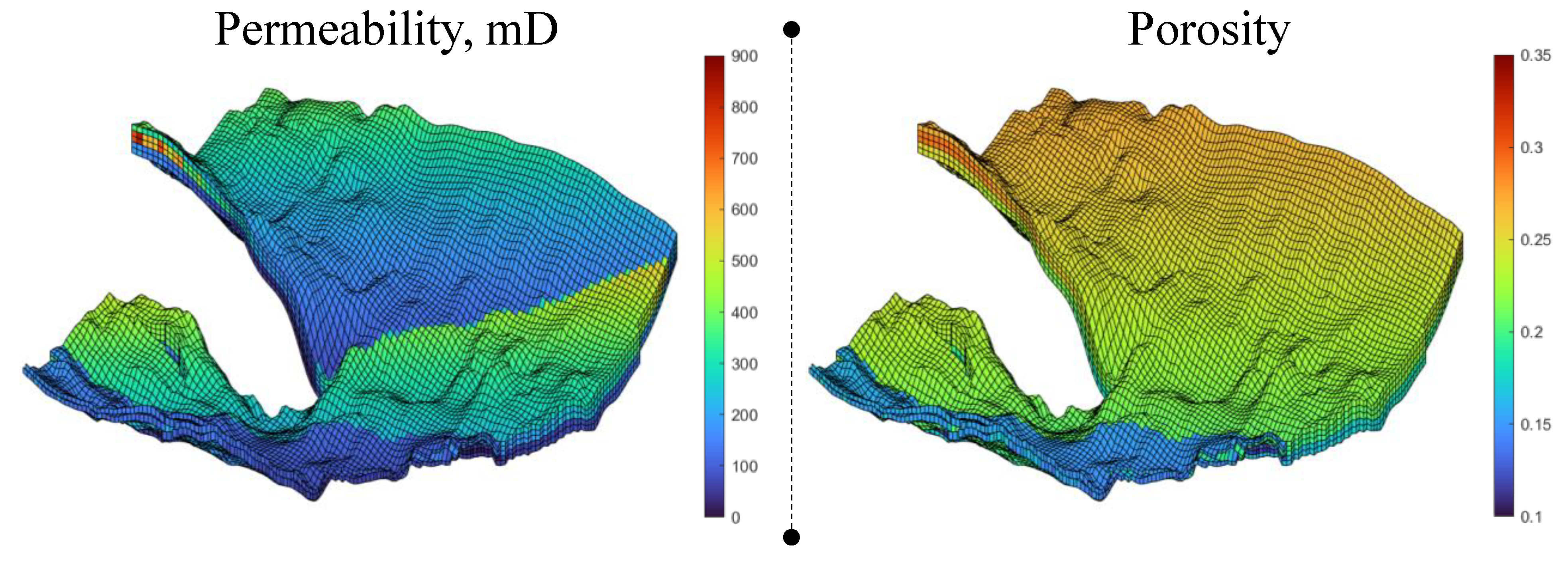
The simulation model consists of 29,128 grid cells. The CO2 injection point was placed in a location where a succession of traps is connected and has a significant trap volume to maximize structural trapping capacity. The formation rock is sandstone with heterogeneous reservoir properties and features a major sealing fault. The fluid and rock properties and the other relevant parameters are listed in Table 1. Figure 2 demonstrates the heterogeneous permeability and porosity models of the Johansen aquifer.

2.4. Proposed Workflow

A ML-based workflow is proposed for modeling field-scale CO2 storage, which overcomes the limitations of extensive simulations of physics-based models. Figure 3 shows the proposed workflow, which includes three steps consisting of (1) dataset generation, (2) ML model development, and (3) uncertainty quantification and global sensitivity analysis, which are detailed as follows.

2.4.1. Step 1: Dataset Generation

First, we identify the uncertainty variables that impact the CO2 trapping capacities and determine their corresponding ranges [54,55]. The Latin Hypercube Sampling (LHS) technique is conducted to create various designs of input samples. LHS assures the sample points are evenly distributed in a space-filling manner across all possible values and avoids bios from data clustering [33,56,57,58,59]. Data clustering may lead to inconsistent accuracy in the model when sampled data points are insufficient for some data intervals and could be oversampled from others. Table 2 summarizes the identified uncertainty parameters and their corresponding ranges. We assume each parameter to be uniformly distributed and independent of the other parameters. In each simulation run, the sampled input data, which comprise the identified uncertainty parameters and the objective outcomes, i.e., trapping capacities, are collected as a training dataset for the next step. The percentages of CO2 entrapments of different mechanisms are calculated by the simulator based on the mobile and residual CO2 saturations.

2.4.2. Step 2: Generate a ML-Based Predictive Model

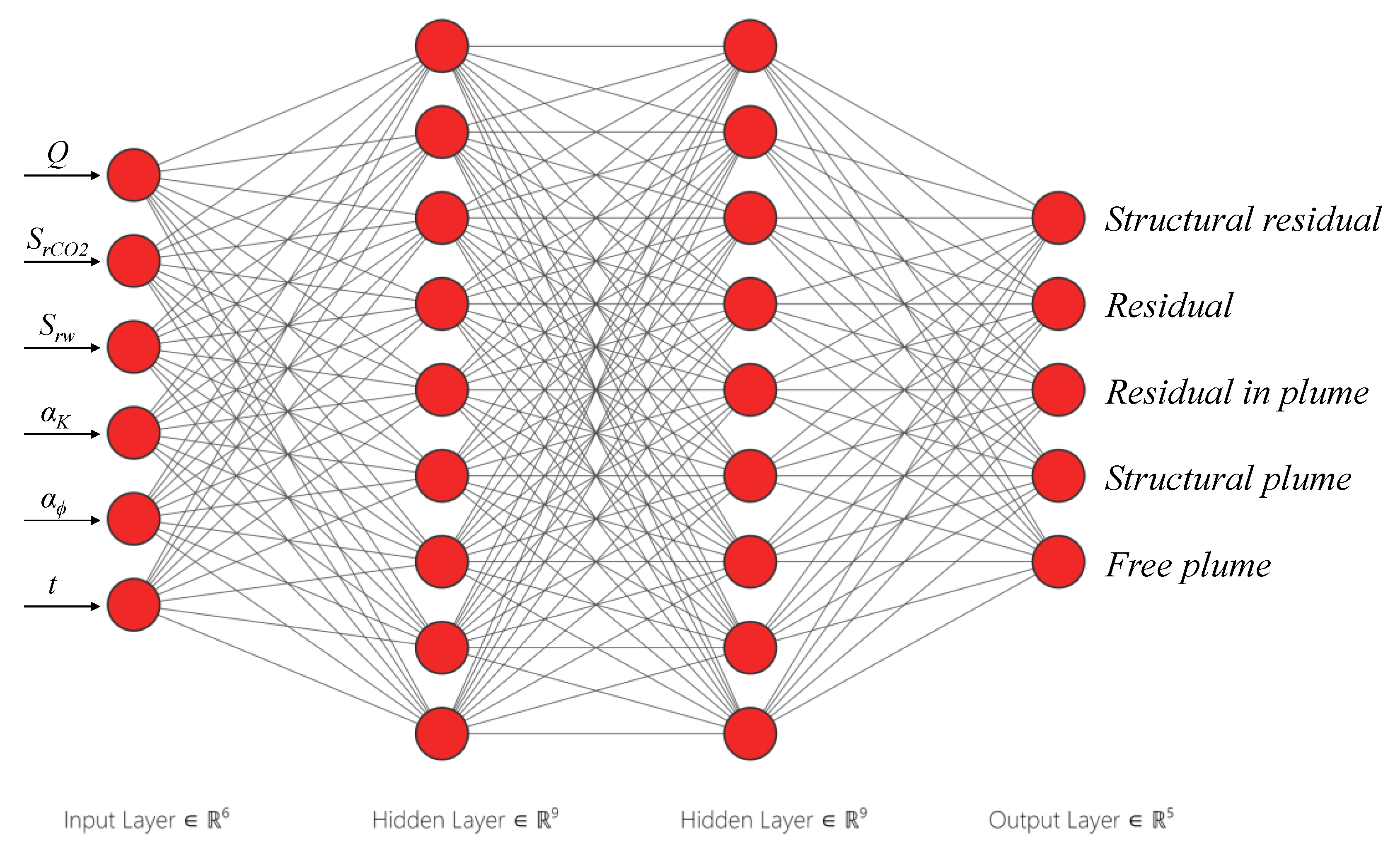
In this step, we developed a data-driven ML model to estimate the nonlinear relationship between the output parameters, i.e., CO2 trapping capacities, and the identified uncertainty variables. This study implemented an Artificial Neural Network (ANN), consisting of three main elements: an input layer, hidden layer(s), and an output layer. The input layer holds a number of neurons corresponding to the number of input features of the problem, i.e., the uncertainty variables and time. ANN with the time term (Figure 4), as an input, can also describe time series problems compared to Long-Short Term Memory (LSTM), yet it honors the simplicity and efficiency of the architecture [57,60]. The output layer contains neurons equal to the number of expected outputs, i.e., the trapping capacities. The hidden layers may have as many layers as the problem dictates. In this problem, we used 3 hidden layers. The ANN model was trained in MATLAB R2022a environment running on an Intel® Xeon® W-2245 CPU 3.91 GHz with 64 GB RAM.
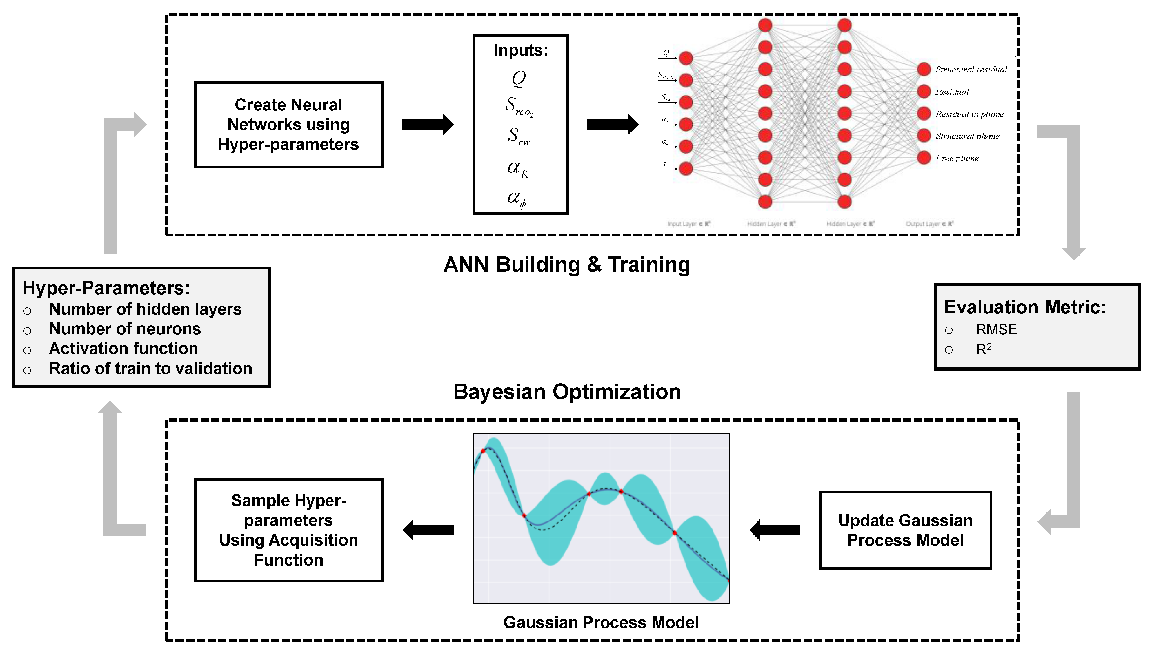
The building and training procedure for the coupled ANN model with Bayesian optimization is illustrated in Figure 5. First, we determine the optimum hyper-parameters of the ANN algorithm, namely the number of hidden layers, the number of neurons in each hidden layer, the type of activation function, and the training–validation–testing ratio.
The training and validation process is then conducted with a target to reach an accuracy of a minimum R2 of 95% for the training and validation steps. To avoid the inefficiencies of manual trial-and-error procedures, we deploy a Bayesian optimization workflow to ensure proper and fast hyper-parameter tuning. With this approach, we update the Gaussian process model and sample the hyper-parameters using the acquisition function. We then reiterate the ANN training process with the updated hyper-parameters until the desired accuracy is achieved. Unlike the traditional trial-and-error process, Bayesian optimization helps automate the hyper-parameter tuning and significantly accelerates the convergence procedure.
There are several statistical indicators used to assess the performance of the developed ML models [51], from which we adopted two evaluation indicators as follows:
  • Root-mean-square Error (RMSE) is the standard deviation of the residuals (prediction errors), which is a measure of the distance of the regression line from the data points. RMSE is given by:
R M S E = i = 1 N ( y i y ¯ ) 2 N
  • Coefficient of determination (R2) is a statistical measure of fit that indicates the amount of variation between actual and predicted values. R2 of 1 means the data are perfectly matched. R2 is calculated using the following equation:
R 2 = 1 i = 1 N ( y i f ( x i ) ) 2 i = 1 N ( y i y ¯ ) 2

2.4.3. Step 3: Uncertainty Quantification and Global Sensitivity Analysis

In this step, we perform Monte Carlo simulations based on the optimized ML model developed in step 2 to explore the uncertainty propagation of time-series outputs for each storage mechanism. The sampled results are collected to quantify the probabilistic percentiles P10, P50, and P90. Eventually, global sensitivity analysis is performed to identify the critical uncertain parameters by calculating the Sobol indices [61,62].

3. Results and Discussion

3.1. Base Case Simulation Result

The base case study consists of a 50-year injection of CO2 followed by a shut-in stage of 450 years of CO2 migration. For a more detailed comparison between different operational scenarios, the conducted simulations quantified CO2 entrapments in six categories, as described below:
  • Structural—CO2 residually trapped inside a structural trap.
  • Residual—CO2 residually trapped outside any structural traps.
  • Residual in the plume fraction of the CO2 plume outside any structural traps will be left behind as residually trapped droplets when the plume migrates away from its current position.
  • Structural plume—mobile CO2 volume that is currently contained within a residual trap; if the containing structure is breached, this volume is free to migrate upward.
  • Free plume—the fraction of the CO2 plume outside of structural traps that is free to migrate upward and/or be displaced by imbibing brine.
  • Exited “leaked”—the volume of CO2 that has leaked out of the domain through its lateral boundaries.
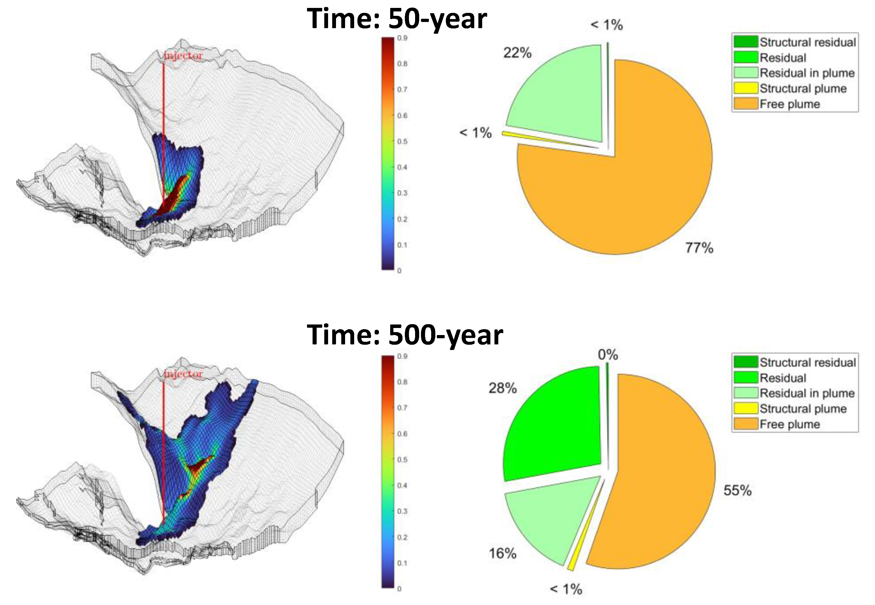
Figure 6 shows the simulation results at the end of the injection period (50 years) and after 500 years, which illustrate the migration of CO2 in the post-injection period and the corresponding evolution of different storage capacities. We notice that the free plume is significantly reduced from 77% to 55%, and the structural residual trap increases by around 28%. Additionally, the residual plume decreases from 22% to 16%. This model has a small contribution from structural traps, while residual trapping is the main entrapping mechanism. Within this simulation time, a small amount of CO2 reaches the top of the structure during the migration timeframe. It should be noted that simulation over a longer period of time could be needed to assess the long-term fate of CO2 migration.

3.2. Generating Training Dataset for the ML Model

Following the base case, a series of simulation scenarios were conducted to generate training data for the ML model. We conducted a total of 100 simulation jobs, each with 95 time steps, using the MRST-CO2lab module. Thus, a total of 9500 input data points were obtained and used to calibrate the ML-ANN model. The data were split into three distinct subgroups according to the train–validation–test ratio. The train split is the set of data on which the actual training takes place. A validation split helps improve the model’s performance by fine-tuning the model. The test split was used to evaluate the model’s performance in terms of accuracy after completing the training phase. The train–validation–test ratio is a critical factor for virtually any ML training process. Generally, the larger the training data split, the more accurate the ML can be. However, the optimum ratio relies upon factors such as the size of the whole dataset, the structure of the model, and the dimension of the data. In this study, the optimized ratio is selected at 0.7:0.15:0.15 for the train, validate, and test splits, respectively, meaning that 70% of the data are used for training, 15% for validating, and the remaining 15% are reserved for testing the model once trained.
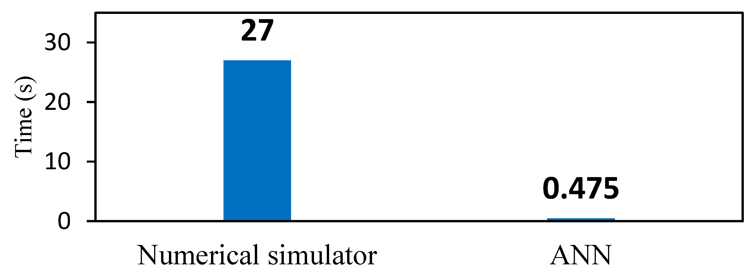
Subsequently, our ANN model was trained with the generated data according to the selected ratio. The ANN fitting function in MATLAB was used to train the model. The Bayesian-optimized hyper-parameters are summarized in Table 3. The optimized ANN architecture consists of three hidden layers with the optimized neurons of 8, 6, and 5, respectively, on each layer. The Sigmoid activation function was found to be the best activation function compared to ReLu and Tanh. Figure 7 shows the computation time for the numerical simulator and the developed ANN model. The reported time is in seconds, and it covers the prediction of CO2 migration mechanisms for 500 years. As can be observed, the ANN outperforms the numerical simulator model by approximately fivefold. This demonstrates the efficiency of the ANN model in accurately reproducing the physics-based model (see Figure 8).
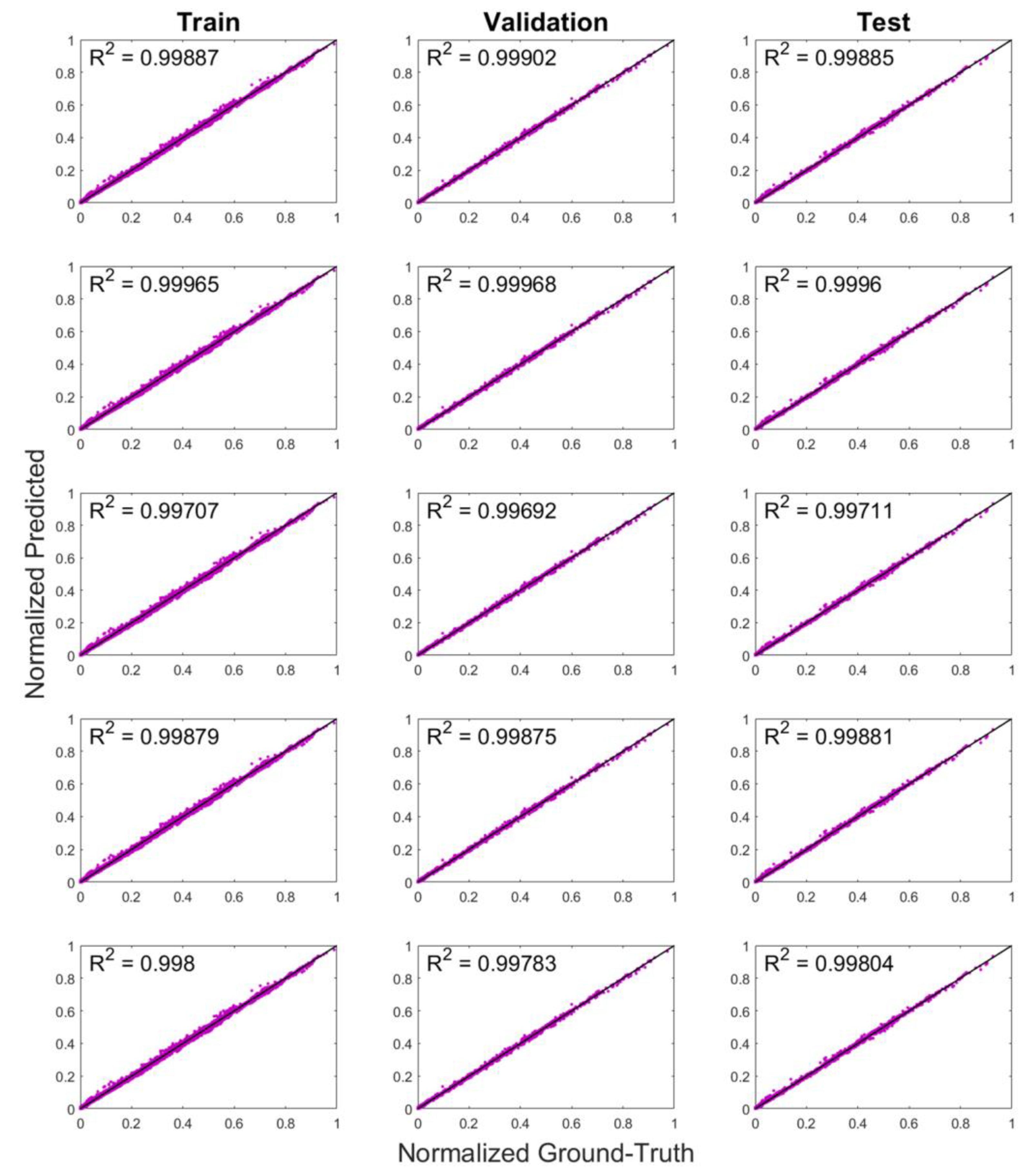
Figure 8 shows the performance of the training, validation, and testing dataset. The diagonal plots compare the normalized ANN predicted results and the ground truth solution. Table 4 shows the statistical indicator of the ANN model. This optimized ANN model is then considered to perform Monte Carlo runs and, eventually, global sensitivity analysis.

3.3. Monte Carlo Simulations

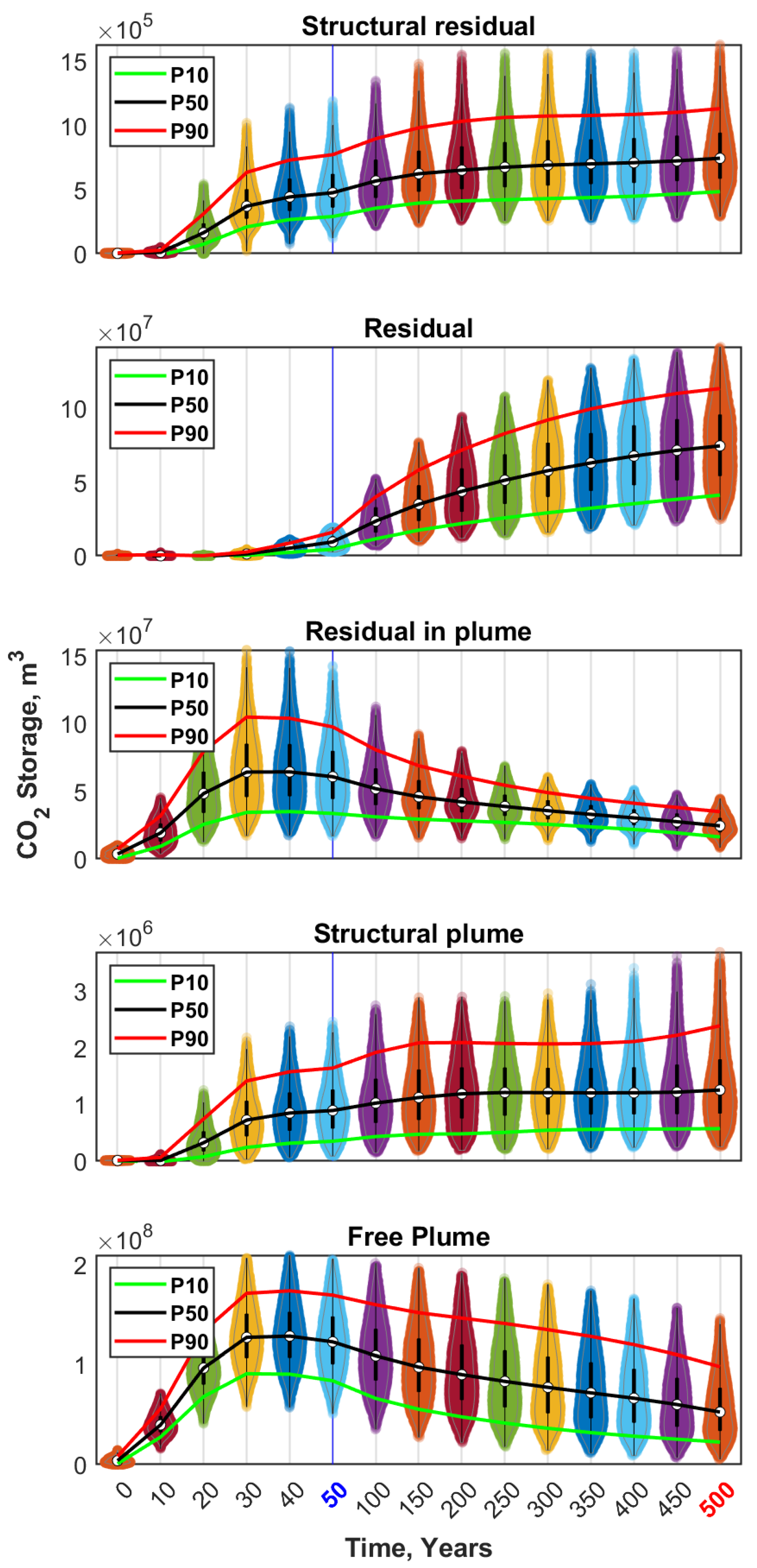
We conducted 5000 Monte Carlo simulations using the trained ANN model to evaluate the uncertainty propagation of the time-series output variations for each type of storage format. The 5000 runs were found to be sufficient to capture the probabilistic distribution. We then grouped the resulting time-series outputs to highlight the percentiles of P10, P50, and P90, as shown in Figure 9.
We observe in the residual plot (second plot) that CO2 storage capacity exhibits two-segment trends—it hardly increases during the first 50-year period (i.e., the injection period) but substantially increases in the post-injection (i.e., the migration) period. In other words, this type of storage capacity does not dominate storage mechanisms in the injection period, yet it starts to play an increasingly important role in the migration period. The residual in the plume (third plot) and free plume (fifth plot) show a different trend, in which the trend increases to reach a peak at or before the injection-stop year during the injection period and then decreases afterward. These trends, based on various Monte Carlo runs, provide guidance for the importance of each storage capacity in different periods.
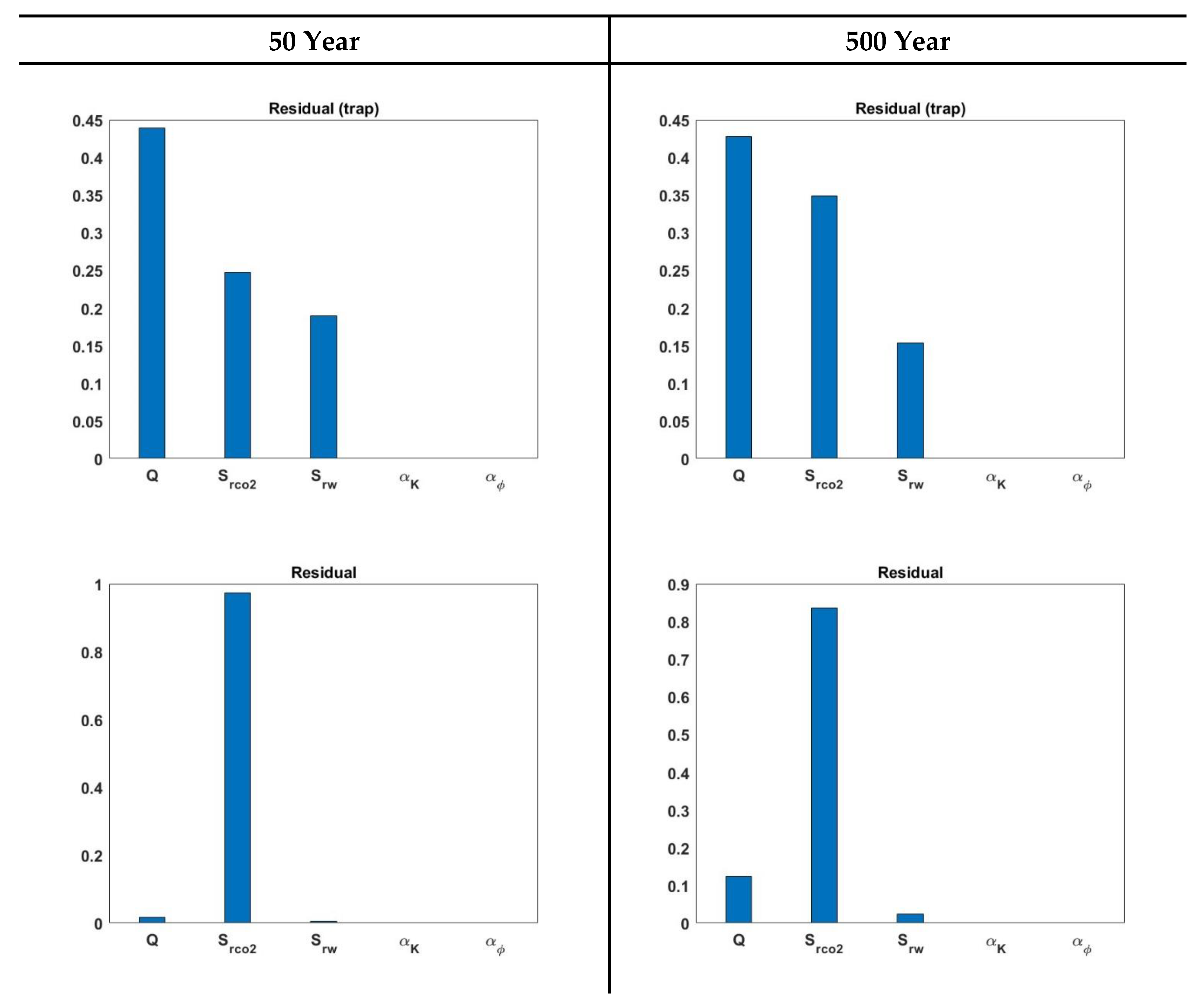
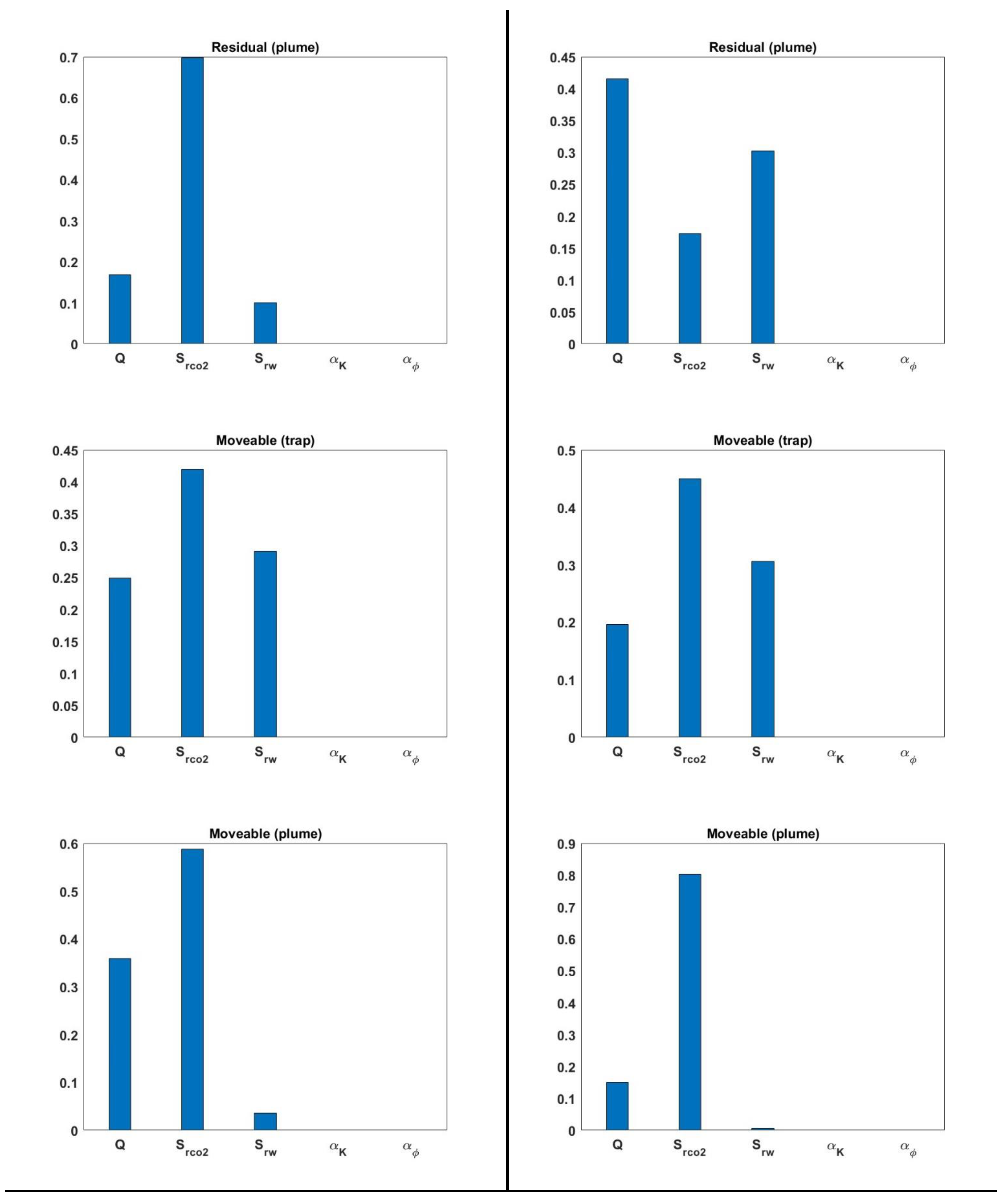
We then conducted a global sensitivity analysis to determine the most significant influential parameters on the investigated outputs by calculating the first-order Sobol indices. The sensitivity analysis was performed within the UQLAB framework [63]. We took the results at 50 and 500 years as references to illustrate the time-series sensitivity analysis. We observe in Figure 10 that in that the permeability and porosity do not show a major influence on the final behavior of CO2 trapping. In the structural (trap) residual (the first row in Figure 9), the CO2 injection rate (Q) significantly influences the storage capacity in the structural residual format at both 50 and 500 years. On the other hand, the residual CO2 saturation (SrCO2) and residual water saturation (Srw) increase to some extent over time. However, in the residual trapping (the second row in Figure 10), Srw dominates the storage mechanism, and its impact slightly decreases within the migration period. Q and Srw showed a weak contribution toward the end of the migration period. The others (third, fourth, and fifth rows) could be observed and summarized in Figure 10. The remaining storage formats (third, fourth, and fifth rows in Figure 10) showed mixed effects in relation to the parameters.

4. Conclusions

This work presents a rigorous machine learning-based workflow for predicting CO2 storage capacity and mechanisms in deep saline aquifers and further conducting uncertainty and global sensitivity analysis. The main findings of this study are summarized as follows:
  • High-resolution numerical simulations (open-source MATLAB package: MRST-CO2lab) are conducted to investigate the various trapping mechanisms and total CO2 storage capacity, where the Johansen Aquifer is used as a real case application in this study. The simulation results are then used as a sample input in the ML model.
  • The ML model, Artificial Neural Network (ANN), with time term as an input coupled with Bayesian optimization, was trained and used to predict the contribution of different trapping mechanisms.
  • The accuracy achieved with the ANN corresponds to RMSE and R2 values of 0.00783 and 0.9988, respectively. Thus, the proposed ML model demonstrates robustness and accuracy in comparison with the numerical reservoir simulator.
  • Monte Carlo simulations with 5000 runs, based on the optimized ML, are performed to explore the uncertainty propagation of time-series model outputs for each storage mechanism. Two distinct trends among the five investigated storage mechanisms are identified, namely residual and free plume mechanisms. The observed trends offer quantitative evaluations for each storage mechanism over different periods.
  • First-order Sobol indices are used to identify the most influential paraments in the model’s predictions. The top three crucial input parameters are injection rate (Q), residual CO2 saturation (SCO2), and water saturation (Srw). Their order of significance varies depending on the specific storage mechanisms. Note that the injection rate is typically a major uncertainty parameter.
  • The conclusions obtained by the global sensitivity analysis offer insights into the most influential time-series contributors, which could ensure better management during large-scale CO2 sequestration.

Author Contributions

Conceptualization, H.H. and X.H.; methodology, A.A.; software, A.A.; validation, X.H., B.Y. and H.H.; formal analysis, A.A.; investigation, A.A.; resources, H.H.; data curation, X.H.; writing—original draft preparation, A.A.; writing—review and editing, X.H., B.Y. and H.H.; visualization, A.A.; supervision, H.H. All authors have read and agreed to the published version of the manuscript.

Funding

This research received no external funding.

Data Availability Statement

All codes are developed in a MATLAB environment and are available upon request ([email protected]).

Acknowledgments

This publication is based upon work supported by the King Abdullah University of Science and Technology (KAUST) Research Funding Office under Award No. 4357.

Conflicts of Interest

The authors declare no conflict of interest.

References

  1. IPCC. Climate Change 2021: The Physical Science Basis. Contribution of Working Group I to the Sixth Assessment Report of the Intergovernmental Panel on Climate Change; Cambridge University Press: Cambridge, UK; New York, NY, USA, 2021; in press. [Google Scholar]
  2. Keeling, C.D.; Bacastow, R.B.; Bainbridge, A.E.; Ekdahl, C.A., Jr.; Guenther, P.R.; Waterman, L.S.; Chin, J.F.S. Atmospheric carbon dioxide variations at Mauna Loa Observatory, Hawaii. Tellus 1976, 28, 538–551. [Google Scholar] [CrossRef]
  3. Metz, B.; Davidson, O.; de Coninck, H.C.; Loos, M.; Meyer, L. IPCC Special Report on Carbon Dioxide Capture and Storage; Cambridge University Press: Cambridge, UK, 2005; ISBN 978-0-521-68551-1. [Google Scholar]
  4. Rose, S.K.; Richels, R.; Blanford, G.; Rutherford, T. The Paris Agreement and next steps in limiting global warming. Clim. Chang. 2017, 142, 255–270. [Google Scholar] [CrossRef]
  5. Hoteit, H.; Fahs, M.; Soltanian, M.R. Assessment of CO2 Injectivity during Sequestration in Depleted Gas Reservoirs. Geosciences 2019, 9, 199. [Google Scholar] [CrossRef]
  6. Underschultz, J.; Boreham, C.; Dance, T.; Stalker, L.; Freifeld, B.; Kirste, D.; Ennis-King, J. CO2 storage in a depleted gas field: An overview of the CO2CRC Otway Project and initial results. Int. J. Greenh. Gas Control. 2011, 5, 922–932. [Google Scholar] [CrossRef]
  7. Iglauer, S. Dissolution Trapping of Carbon Dioxide in Reservoir Formation Brine—A Carbon Storage Mechanism; IntechOpen: Rijeka, Croatia, 2011; ISBN 978-953-307-636-2. [Google Scholar]
  8. Nilsen, H.M.; Lie, K.-A.; Andersen, O. Fully-implicit simulation of vertical-equilibrium models with hysteresis and capillary fringe. Comput. Geosci. 2016, 20, 49–67. [Google Scholar] [CrossRef]
  9. White, C.M.; Smith, D.H.; Jones, K.L.; Goodman, A.L.; Jikich, S.A.; LaCount, R.B.; DuBose, S.B.; Ozdemir, E.; Morsi, B.I.; Schroeder, K.T. Sequestration of Carbon Dioxide in Coal with Enhanced Coalbed Methane RecoveryA Review. Energy Fuels 2005, 19, 659–724. [Google Scholar] [CrossRef]
  10. IEA. CO2 Storage in Depleted Gas Field; IEA: Paris, France, 2009. [Google Scholar]
  11. Arkadakskiy, S.; Oelkers, E.H.; Afifi, A.; Hoteit, H.; Gislason, S.R.; Kunnummal, N.; Ahmed, Z. The Potential for Sequestering CO2 in Basalts along the Red Sea Coast of Saudi Arabia. In Proceedings of the AGU Fall Meeting Abstracts, Chicago, IL, USA, 12–16 December 2020; Volume 2020, p. GC111-05. [Google Scholar]
  12. Oelkers, E.H.; Arkadakskiy, S.; Afifi, A.M.; Hoteit, H.; Richards, M.; Fedorik, J.; Delaunay, A.; Torres, J.E.; Ahmed, Z.T.; Kunnummal, N.; et al. The subsurface carbonation potential of basaltic rocks from the Jizan region of Southwest Saudi Arabia. Int. J. Greenh. Gas Control. 2022, 120, 103772. [Google Scholar] [CrossRef]
  13. Hoteit, H.; Addassi, M. Integrated Uncertainty Quantification for Reactive Transport Modeling of CO2 Mineralization in Basalts. 3rd EAGE Geochem. Workshop 2021, 2021, 1–5. [Google Scholar] [CrossRef]
  14. Javaheri, M.; Abedi, J.; Hassanzadeh, H. Onset of Convection in CO2 Sequestration in Deep Inclined Saline Aquifers. J. Can. Pet. Technol. 2009, 48, 22–27. [Google Scholar] [CrossRef]
  15. Hamieh, A.; Rowaihy, F.; Al-Juaied, M.; Abo-Khatwa, A.N.; Afifi, A.M.; Hoteit, H. Quantification and analysis of CO2 footprint from industrial facilities in Saudi Arabia. Energy Convers. Manag. X 2022, 16, 100299. [Google Scholar] [CrossRef]
  16. Corrales, M.; Mantilla Salas, S.; Tasianas, A.; Hoteit, H.; Afifi, A. The Potential for Underground CO2 Disposal Near Riyadh. In Proceedings of the International Petroleum Technology Conference, Riyadh, Saudi Arabia, 21–23 February 2022; OnePetro: Riyadh, Saudi Arabia, 2022. [Google Scholar]
  17. Temitope, A.; Gomes, J.S.; Al Kobaisi, M.; Hu, J. Characterization and Quantification of the CO2 Sequestration Potential of a Carbonate Aquifer in Falaha Syncline, Onshore Abu Dhabi; OnePetro: Abu Dhabi, United Arab Emirates, 2016. [Google Scholar]
  18. Zhang, H.; Arif, M.; Al Kobaisi, M. A Numerical Evaluation of the Impact of Wettability on CO2 Trapping Capacity: Implications for Carbon Geo-Sequestration; OnePetro: Abu Dhabi, United Arab Emirates, 2022. [Google Scholar]
  19. Wang, Y.; Vuik, C.; Hajibeygi, H. Analysis of hydrodynamic trapping interactions during full-cycle injection and migration of CO2 in deep saline aquifers. Adv. Water Resour. 2022, 159, 104073. [Google Scholar] [CrossRef]
  20. Kumar, A.; Noh, M.; Ozah, R.; Pope, G.; Bryant, S.; Sepehrnoori, K.; Lake, L. Reservoir Simulation of CO2 Storage in Deep Saline Aquifers. SPE J. 2005, 10, 336–348. [Google Scholar] [CrossRef]
  21. Ali, M.; Yekeen, N.; Pal, N.; Keshavarz, A.; Iglauer, S.; Hoteit, H. Influence of pressure, temperature and organic surface concentration on hydrogen wettability of caprock; implications for hydrogen geo-storage. Energy Rep. 2021, 7, 5988–5996. [Google Scholar] [CrossRef]
  22. Omar, A.; Addassi, M.; Vahrenkamp, V.; Hoteit, H. Co-Optimization of CO2 Storage and Enhanced Gas Recovery Using Carbonated Water and Supercritical CO2. Energies 2021, 14, 7495. [Google Scholar] [CrossRef]
  23. Clavijo, S.P.; Addassi, M.; Finkbeiner, T.; Hoteit, H. A coupled phase-field and reactive-transport framework for fracture propagation in poroelastic media. Sci. Rep. 2022, 12, 17819. [Google Scholar] [CrossRef]
  24. Shafabakhsh, P.; Ataie-Ashtiani, B.; Simmons, C.T.; Younes, A.; Fahs, M. Convective-reactive transport of dissolved CO2 in fractured-geological formations. Int. J. Greenh. Gas Control. 2021, 109, 103365. [Google Scholar] [CrossRef]
  25. Soltanian, M.R.; Amooie, M.A.; Gershenzon, N.; Dai, Z.; Ritzi, R.; Xiong, F.; Cole, D.; Moortgat, J. Dissolution Trapping of Carbon Dioxide in Heterogeneous Aquifers. Environ. Sci. Technol. 2017, 51, 7732–7741. [Google Scholar] [CrossRef]
  26. Addassi, M.; Omar, A.; Ghorayeb, K.; Hoteit, H. Comparison of various reactive transport simulators for geological carbon sequestration. Int. J. Greenh. Gas Control. 2021, 110, 103419. [Google Scholar] [CrossRef]
  27. Addassi, M.; Omar, A.; Hoteit, H.; Alafifi, A.M.; Arkadakskiy, S.; Ahmed, Z.T.; Kunnummal, N.; Gislason, S.R.; Oelkers, E.H. Assessing the potential of solubility trapping in unconfined aquifers for subsurface carbon storage. Sci. Rep. 2022, 12, 20452. [Google Scholar]
  28. Ali, M.; Yekeen, N.; Pal, N.; Keshavarz, A.; Iglauer, S.; Hoteit, H. Influence of organic molecules on wetting characteristics of mica/H2/brine systems: Implications for hydrogen structural trapping capacities. J. Colloid Interface Sci. 2022, 608, 1739–1749. [Google Scholar] [CrossRef]
  29. Ahmadi, M.A.; Chen, Z. Analytical Model for Leakage Detection in CO2 Sequestration in Deep Saline Aquifers: Application to ex Situ and in Situ CO2 Sequestration Processes. ACS Omega 2019, 4, 21381–21394. [Google Scholar] [CrossRef] [PubMed] [Green Version]
  30. Qiao, T.; Hoteit, H.; Fahs, M. Semi-Analytical Solution to Assess CO2 Leakage in the Subsurface through Abandoned Wells. Energies 2021, 14, 2452. [Google Scholar] [CrossRef]
  31. Hesse, M.A.; Tchelepi, H.A.; Orr, F.M. Scaling Analysis of the Migration of CO2 in Saline Aquifers; OnePetro: San Antonio, TX, USA, 2006. [Google Scholar]
  32. Zhang, Z.; He, X.; AlSinan, M.; Li, Y.; Kwak, H.; Hoteit, H. Deep Learning Model for CO2 Leakage Detection Using Pressure Measurements. In Proceedings of the SPE Annual Technical Conference and Exhibition; OnePetro: Houston, TX, USA, 2022. [Google Scholar]
  33. He, X.; Zhu, W.; Santoso, R.; Alsinan, M.; Kwak, H.; Hoteit, H. CO2 Leakage Rate Forecasting Using Optimized Deep Learning; OnePetro: Dubai, United Arab Emirates, 2021. [Google Scholar]
  34. Yan, B.; Harp, D.R.; Chen, B.; Hoteit, H.; Pawar, R.J. A gradient-based deep neural network model for simulating multiphase flow in porous media. J. Comput. Phys. 2022, 463, 111277. [Google Scholar]
  35. Santoso, R.; He, X.; Hoteit, H. Application of machine-learning to construct simulation models from high-resolution fractured formation. In Proceedings of the Society of Petroleum Engineers—Abu Dhabi International Petroleum Exhibition and Conference, Abu Dhabi, United Arab Emirates, 11–14 November 2019. [Google Scholar] [CrossRef]
  36. Li, H.; Gong, C.; Liu, S.; Xu, J.; Imani, G. Machine Learning-Assisted Prediction of Oil Production and CO2 Storage Effect in CO2-Water-Alternating-Gas Injection (CO2-WAG). Appl. Sci. 2022, 12, 10958. [Google Scholar] [CrossRef]
  37. Ahmadi, M.A.; Zendehboudi, S.; James, L.A. Developing a robust proxy model of CO2 injection: Coupling Box–Behnken design and a connectionist method. Fuel 2018, 215, 904–914. [Google Scholar] [CrossRef]
  38. Al-Mudhafar, W.J. Polynomial and nonparametric regressions for efficient predictive proxy metamodeling: Application through the CO2-EOR in shale oil reservoirs. J. Nat. Gas Sci. Eng. 2019, 72, 103038. [Google Scholar] [CrossRef]
  39. You, J.; Ampomah, W.; Sun, Q.; Kutsienyo, E.J.; Balch, R.S.; Dai, Z.; Cather, M.; Zhang, X. Machine learning based co-optimization of carbon dioxide sequestration and oil recovery in CO2-EOR project. J. Clean. Prod. 2020, 260, 120866. [Google Scholar] [CrossRef]
  40. Vo Thanh, H.; Lee, K.-K. Application of machine learning to predict CO2 trapping performance in deep saline aquifers. Energy 2022, 239, 122457. [Google Scholar] [CrossRef]
  41. Riis, F.; Halland, E. CO2 Storage Atlas of the Norwegian Continental Shelf: Methods Used to Evaluate Capacity and Maturity of the CO2 Storage Potential. Energy Procedia 2014, 63, 5258–5265. [Google Scholar] [CrossRef]
  42. SINTEF The MATLAB Reservoir Simulation Toolbox (MRST). MRST 2015. Available online: https://www.sintef.no/projectweb/mrst/ (accessed on 1 December 2022).
  43. Lie, K.-A. An Introduction to Reservoir Simulation Using MATLAB/GNU Octave: User Guide for the MATLAB Reservoir Simulation Toolbox (MRST); Cambridge University Press: Cambridge, UK, 2019; ISBN 978-1-108-49243-0. [Google Scholar]
  44. Ahmed, T.; Nasrabadi, H.; Firoozabadi, A. Complex Flow and Composition Path in CO2 Injection Schemes from Density Effects. Energy Fuels 2012, 26, 4590–4598. [Google Scholar] [CrossRef]
  45. Nordbotten, J.M.; Flemisch, B.; Gasda, S.E.; Nilsen, H.M.; Fan, Y.; Pickup, G.E.; Wiese, B.; Celia, M.A.; Dahle, H.K.; Eigestad, G.T.; et al. Uncertainties in practical simulation of CO2 storage. Int. J. Greenh. Gas Control. 2012, 9, 234–242. [Google Scholar] [CrossRef]
  46. Jan Martin Nordbotten, M.A.C. Geological Storage of CO2: Modeling Approaches for Large-Scale Simulation, 1st ed.; Wiley: New York, NY, USA, 2011; ISBN 0-470-88946-2. [Google Scholar]
  47. Ligaarden, I.; Nilsen, H. Numerical Aspects of Using Vertical Equilibrium Models for Simulating CO2 Sequestration. In Proceedings of the ECMOR 12th European Conference on the Mathematics of Oil Recovery, Oxford, UK, 6–9 September 2010. [Google Scholar] [CrossRef]
  48. Span, R.; Wagner, W. A New Equation of State for Carbon Dioxide Covering the Fluid Region from the Triple-Point Temperature to 1100 K at Pressures up to 800 MPa. J. Phys. Chem. Ref. Data 1996, 25, 1509–1596. [Google Scholar] [CrossRef]
  49. Nilsen, H.M.; Lie, K.-A.; Andersen, O. Robust simulation of sharp-interface models for fast estimation of CO2 trapping capacity in large-scale aquifer systems. Comput. Geosci. 2016, 20, 93–113. [Google Scholar] [CrossRef]
  50. Alqahtani, A.S. New Polymer Rheology Models Based on Machine Learning. Master’s Thesis, the University of Texas at Austin, Austin, TX, USA, 2019. [Google Scholar]
  51. Norvig, P.; Russell, S. Artificial Intelligence: A Modern Approach; Pearson Education: London, UK, 2011; ISBN 978-0-13-300198-3. [Google Scholar]
  52. SINTEF the MATLAB Reservoir Simulation Toolbox: Numerical CO2 Laboratory. MRST-co2lab 2014.
  53. Halland, E.; Mujezinović, J.; Riis, F. CO2 Storage Atlas: Norwegian Continental Shelf; The Norwegian Petroleum Directorate: Stavanger, Norway, 2014. [Google Scholar]
  54. Abbaszadeh, M.; Shariatipour, S.M. Investigating the Impact of Reservoir Properties and Injection Parameters on Carbon Dioxide Dissolution in Saline Aquifers. Fluids 2018, 3, 76. [Google Scholar] [CrossRef]
  55. Liu, B.; Zhang, Y. CO2 Modeling in a Deep Saline Aquifer: A Predictive Uncertainty Analysis Using Design of Experiment. Environ. Sci. Technol. 2011, 45, 3504–3510. [Google Scholar] [CrossRef] [PubMed]
  56. Stein, M. Large sample properties of simulations using latin hypercube sampling. Technometrics 1987, 29, 143–151. [Google Scholar] [CrossRef]
  57. He, X.; Santoso, R.; Alsinan, M.; Kwak, H.; Hoteit, H. Constructing Dual-Porosity Models from High-Resolution Discrete-Fracture Models Using Deep Neural Networks; OnePetro: Richardson, TX, USA, 2021. [Google Scholar]
  58. Santoso, R.; Hoteit, H.; Vahrenkamp, V. Optimization of energy recovery from geothermal reservoirs undergoing re-injection: Conceptual application in Saudi Arabia. In Proceedings of the SPE Middle East Oil and Gas Show and Conference, MEOS, Manama, Bahrain, 18–21 March 2019; Society of Petroleum Engineers (SPE): Houston, TX, USA, 2019; Volume 2019. [Google Scholar]
  59. Santoso, R.; Torrealba, V.; Hoteit, H. Investigation of an improved polymer flooding scheme by compositionally-tuned slugs. Processes 2020, 8, 197. [Google Scholar]
  60. Kim, Y.; Jang, H.; Kim, J.; Lee, J. Prediction of storage efficiency on CO2 sequestration in deep saline aquifers using artificial neural network. Appl. Energy 2017, 185, 916–928. [Google Scholar] [CrossRef]
  61. Marelli, S.; Sudret, B. UQLab: A Framework for Uncertainty Quantification in Matlab. In Vulnerability, Uncertainty, and Risk: Quantification, Mitigation, and Management; American Society of Civil Engineers: Reston, VA, USA, 2014. [Google Scholar]
  62. Sahu, Q.; Fahs, M.; Hoteit, H. Optimization and Uncertainty Quantification Method for Reservoir Stimulation through Carbonate Acidizing. ACS Omega 2023, 8, 539–554. [Google Scholar] [CrossRef]
  63. Marelli, S.; Lamas, C.; Sudret, B. UQLab User Manual—Sensitivity Analysis. Rep. UQLab-V1 2015, 2–106. [Google Scholar] [CrossRef]
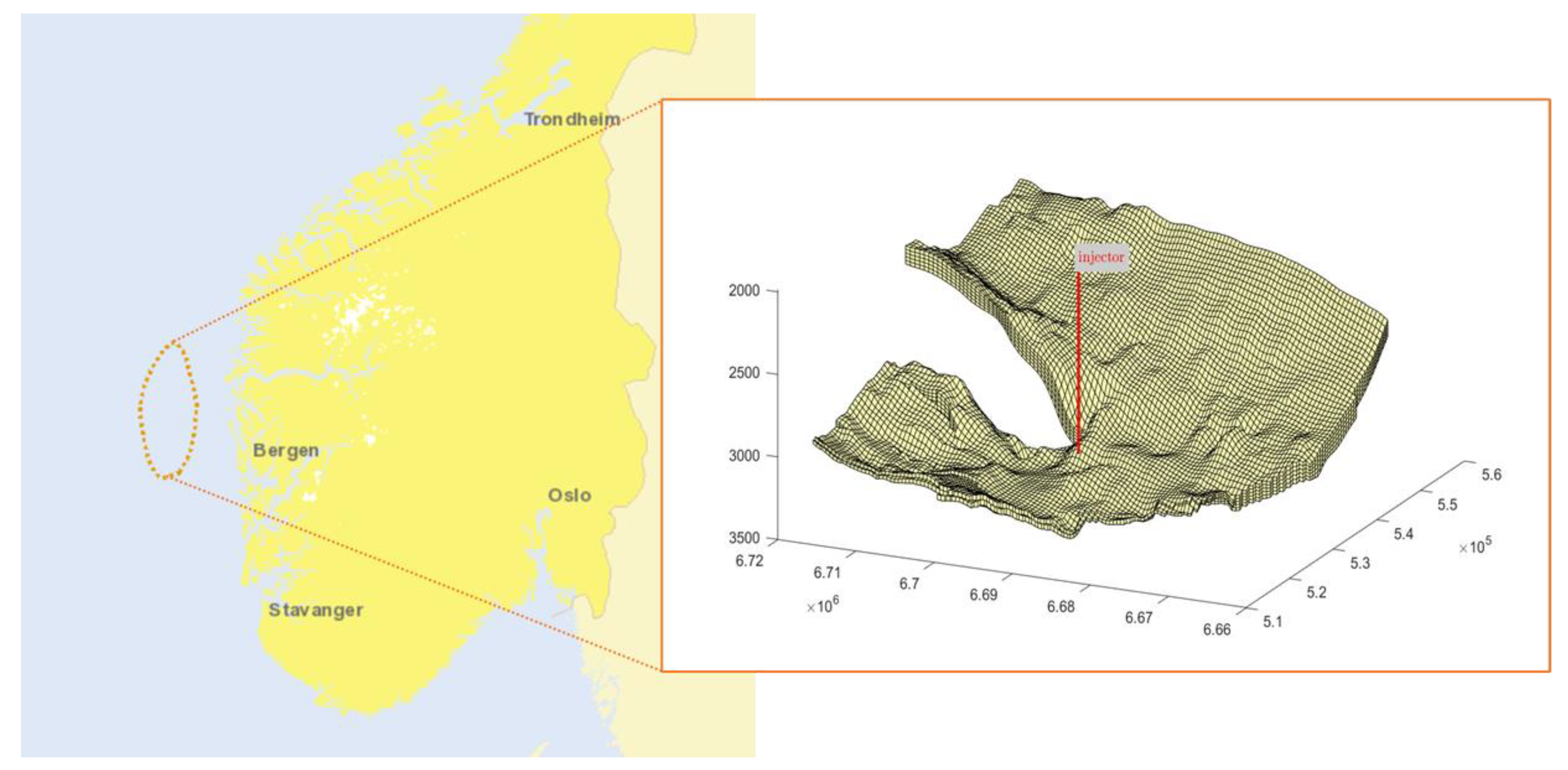
Figure 1. The location and the geological model of the Johansen aquifer with the well location [53].
Energies 16 01684 g001
Figure 2. The permeability (left) and porosity (right) 3D maps of the Johansen aquifer.
Energies 16 01684 g002
Figure 3. The proposed workflow for performing uncertainty and global sensitivity analysis for CO2 Storage in a saline aquifer.
Energies 16 01684 g003
Figure 4. Schematic showing our ANN model architecture, including input, hidden, and output layers.
Energies 16 01684 g004
Figure 5. The process of ANN training with Bayesian optimization.
Energies 16 01684 g005
Figure 6. CO2 saturation profiles and the corresponding trapping inventory diagrams at different times.
Energies 16 01684 g006
Figure 7. Computation time of numerical simulator and ANN model.
Energies 16 01684 g007
Figure 8. Parity plots show the performance of the ANN model, which compares the prediction results with the ground-truth (simulation) results. The first row of plots corresponds to structural residual trapping, the second row to residual trapping, the third row to residual trapping in the plume, the fourth to structural trapping in the plume, and the last row to the free plume.
Energies 16 01684 g008
Figure 9. Uncertainty analysis based on 5000 Monte Carlo simulations for time-series outputs.
Energies 16 01684 g009
Figure 10. Global sensitivity analysis by calculating the first-order Sobol indices to determine the key contributors to the time-continuous outputs.
Energies 16 01684 g010aEnergies 16 01684 g010b
Table 1. The simulation parameters and corresponding values for the base case.
ParameterBase Case Value
CO2 injection rate Q8000 m3/day
Residual CO2 saturation Srco2 0.2
Residual water saturation Srw0.1
Permeability K233 mD (Avg.)
Porosity ϕ 22% (Avg.)
Fluid propertiesρco2 = 686.54   ρw = 975.86 kg/m3
μco2 = 0.056641   μw = 0.30860 cp
Injection period50 years
Post-injection (migration) period450 years
Table 2. The uncertainty parameters considered for this study with corresponding ranges.
Uncertainty ParametersLower BoundUpper Bound
CO2 injection rate Q8000 m3/day14,000 m3/day
Residual CO2 saturation Srco2 0.10.4
Residual water saturation Srw0.10.4
Permeability coefficient αK0.81.4
Porosity coefficient αϕ0.81.4
Table 3. The optimized hyper-parameters for the ANN model.
Tuned Hyper-ParameterANN
Number of hidden layers3
Neurons per hidden layer[8 6 5]
Activation FunctionSigmoid
Table 4. The statistical indicator shows the performance of the ANN model.
IndicatorTrainValidationTest
RMSE0.007970.008080.00783
R20.99880.99880.9988
Disclaimer/Publisher’s Note: The statements, opinions and data contained in all publications are solely those of the individual author(s) and contributor(s) and not of MDPI and/or the editor(s). MDPI and/or the editor(s) disclaim responsibility for any injury to people or property resulting from any ideas, methods, instructions or products referred to in the content.