Abstract
The main goal of this paper is to research and analyze the problem of image reconstruction performance using machine learning methods in 3D electrical capacitance tomography (ECT) and electrical impedance tomography (EIT) by comparing the areas inside the tank to determine the finite elements for which one of the method reconstructions is more effective. The research was conducted on 5000 simulated cases, which ranged from one to five inclusions generated for a cylindrical tank. The authors first used the elastic net learning method to perform the reconstruction and then proposed a method for testing the effectiveness of reconstruction. Based on this approach, the reconstructions obtained by each method were compared, and the areas within the object were identified. Finally, the results obtained from the simulation tests were verified on real measurements made with two types of tomographs. It was found that areas closer to the edge of the tank were more effectively reconstructed by EIT, while ECT reconstructed areas closer to the center of the tank. Extensive analysis of the inclusions makes it possible to use this measurement for energy optimization of industrial processes and biogas plant operation.
1. Introduction
Tomography is often used for energy optimization of industrial and technological processes. It is also used in monitoring for the detection and prevention of accidents. Due to the ability to reconstruct the interior of objects using measurements only at the boundary of the object, tomography provides a non-invasive method of controlling the flow of liquids or gases in pipes. It can also be used to control the formation of crystals or gas bubbles in industrial reactors. The advantage of tomography is primarily its non-invasiveness. The presence of detectors or sensors inside the controlled object can disrupt the control of processes by invasive methods. Such a measurement can not only interfere with the production process but can also be subject to error due to the interference associated with the invasiveness of the method. Tomography has been used to control processes in industrial reactors [1,2], control the flow of liquids or gases in pipes [3,4], detect moisture in building walls [5,6], flood embankments leaks [7,8], monitor health [9,10], etc.
Advanced measurement techniques and modern IT tools [11,12,13,14,15] allow the monitoring of processes in real-time, providing the possibility of dynamic control of the processes and rapid diagnosis of defects. Measuring devices for industrial tomography are constantly being developed and are subject to the focus of scientific research [16,17,18,19].
The best-known tomographic method is computed tomography (CT) in medical applications. However, in recent years, the trend of industrial tomography has grown due to the development of technology.
Electrical impedance tomography is a non-invasive tomographic method used in industry and medicine. Reconstruction of the interior of the test object is carried out by measuring the voltage between electrodes placed on its edge [20]. Electrical capacitance tomography is a technique that allows spatial visualization of the interior of the examined object. Reconstruction is based on measurements of the mutual capacitance of electrodes placed on the surface of the test object [3,19,21,22,23,24]. Electrical resistivity tomography (ERT) is a technique that allows imaging using electrical resistivity measurements taken at the surface or through electrodes in one or more holes, such as in soil [7,25,26]. In addition to the mentioned types of tomography, there are several tomography methods using physical phenomena such as X-ray [27], sound waves [28], magnetism [29], etc.
The inverse problem is solved using deterministic or machine learning methods in computed tomography. Deterministic methods include the Total Variation Method [30] and Gauss-Newton with Tikhonov penalization [31]. Machine learning methods include neural networks [32], elastic net [33], logistic regression [4], etc. A comparison of the reconstruction quality using different methods can be found in the work [34,35].
Currently, there are two trends in the development of medical computed tomography. First is expanding databases and improving machine-learning algorithms to optimize automatic-disease detection and classification of tomographic images [36,37,38,39]. Second is the improvement in diagnostic tools such as microwave tomography [40,41], ultrasound tomography (UST) [42,43], and electrical tomography [44,45,46].
There are also two trends being actively developed in industrial tomography. First, on reconstruction algorithms in tomography based on neural networks, convolutional neural networks and machine learning algorithms [47,48,49,50] are being optimized. Others being EIT [51,52], ECT [14,53,54], or hybrid tomography devices that are being developed [54,55,56].
The quality of reconstruction in computed tomography depends on many factors. For example, the number of measuring electrodes, the tools used to solve the inverse problem, or the type of tomography used. When comparing the types of tomography with each other, it turns out hybrid methods often do not improve image reconstruction. In the article [56] in which the authors compare imaging with UST and EIT, both methods’ image reconstruction quality was examined. It was found that for a method using simultaneous measurements from both types of tomography, the algorithm used the averages of measurements from both methods. As a result, worse results are obtained for some images rather than those using only one method.
The motivation for undertaking the research included in the paper was to see which areas inside the object under study are reconstructed better by a particular tomography method. Since reconstructing images in hybrid tomography based on a combined observation matrix often yields worse reconstructions than individual methods [56], this paper examines how electrical tomography methods reconstruct individual areas inside the tank.
The main difference of measurement in tomographs is not only the physical phenomenon that is used in tomography, i.e., the way the interior of the reconstructed object is exciting, but also the way the signal propagating inside is measured. The physics of the phenomenon usually forces the method of measurement. The variation in the reconstruction quality inside the object depends on the electric field propagating inside the object between the transmitting and receiving electrodes. In addition, the mechanism of energy dissipation of the electric field caused by the presence of inclusions, which interfere with the propagation of the signal, has a payoff. The reconstruction capability will depend on the magnitude of the conversion of electric field energy to thermal energy (absorption), and the arrangement of the measuring electrodes. Therefore, the study was conducted for two types of 3D tomography. The comparison was made on simulation data, where the elastic net machine learning algorithm was used to solve the inverse problem. The paper [52] made comparisons of machine-learning algorithms used in reconstruction with EIT. Comparisons were made between ANNs, convolutional networks, support vector machine, and elastic net. It was found that convolutional networks are the best among the algorithms (giving the best reconstruction quality). On the other hand, the elastic net algorithm gave worse reconstructions but good quality.
This paper aims to determine the sensitivity areas of ECT and EIT in order to develop a hybrid method for image reconstruction. First, these areas are determined based on the parameter proposed in the paper. Then, the results obtained from simulation data were verified on real measurements and reconstructions.
Similar Research
In [56], authors explored the area of hybrid tomography for measuring humidity in the walls using capacitance and impedance tomography. The most significant difference is that no machine-learning method was used in the paper, and the authors did not study the sensitivity areas of the methods.
In contrast to the cheap method presented in the paper, it is also worth noting that hybrid tomography that describes electrical properties (permittivity and conductivity) was studied in [57] with magnetic resonance. The problem with this method is that it is not easily scalable; it is also expensive in industrial applications.
The paper by Wang [58] explored the topic of hybrid electrical capacitance and resistance tomography. The study was focused on moisture-content detection by these two techniques. This work was performed with deterministic methods using only eight electrodes.
In the paper [59], the authors used a method that combines neural networks with restricted Boltzmann machine (RBM) autoencoder in electromagnetic tomography technology (EMT) to reconstruct images. The proposed algorithm was compared with Landweber’s iterative algorithm and local binary prescription algorithms for solving the inverse problem, and better reconstruction results were obtained concerning inter correlation coefficient (ICC), among others. At the same time, it was noted that the method learns better on more extensive and diverse sets.
In [60], the authors summarized the most current and evolving reconstruction algorithms in EIT tomography. Linear algorithms such as the paper present a new method for accurate reconstruction of the region of interest (ROI) based on regular wavelets iterative reconstruction procedure. Non-linear algorithms such as D-bar (low-pass filtering on the Fourier decomposition) and its improvements with CNNs while pointing out its limitations in application to 3D imaging or sparse Bayesian learning algorithms based on structural sparsity of the conductivity distribution was used. The authors compare the algorithms with each other pointing out their advantages and disadvantages but do not compare the algorithms on datasets.
The paper [61] compared LSTM and CNN machine-learning algorithms for reconstructing moisture inside the walls. It was obtained that the reconstruction algorithm using LSTM proved to be more efficient in terms of reconstruction than CNN in half of the cases.
In the paper [62], super-resolution methodology techniques were considered to improve the quality of the obtained images. It was observed that the super-resolution algorithm improves the quality of image reconstruction in EIT tomography.
The paper [63] compares radial basis neural networks (RBNN) and Hopfield neural networks (HNN) reconstruction algorithms for EIT tomography. Furthermore, these neural networks are compared with the Gauss-Newton (GN) algorithm. As a result of the comparison, it was obtained that concerning the MSE criterion, RBNN and HNN over the GN algorithm had better reconstruction quality.
The paper [64] proposes a reconstruction approach using autoencoders and deep self-training neural networks. The reconstruction method was designed by approximating sinograms using a set of randomly weighted neural networks (extreme learning machines) from potential electrical data. The system was trained on simulated images and compared with the method without autoencoders.
In [65], authors compared two ANN neural network architectures based on LeNet, the other feed-forward fully connected ANN. The comparison was based on simulated data and obtained better reconstruction quality for LeNet architecture.
The paper [66] proposed a method for optimizing machine learning algorithms in complex pixel-oriented ensemble method (POE) reconstruction. For each pixel, the reconstruction was performed with one of the algorithms elastic net, linear regression with the least-squares learner (LR-LS), linear regression with SVM learner (LR-SVM), and artificial neural networks (ANN); then, the reconstructions were optimized by selecting the best algorithms for each area. For the highest number of pixels, ANN was selected as the best algorithm, and in second place was elastic net, LR-LS, and LR-SVM.
The paper [67] proposed a two-stage reconstruction learning process. The proposed method consists of a pre-construction block and a convolutional neural network (CNN). First, the pre-construction block learns the regularization pattern from the training data set and provides an approximate reconstruction of the target. The CNN then processes the results of the initial reconstruction and eliminates modeling errors due to prior information about the shape of the observation domain.
2. Materials and Methods
The study was performed using electrical impedance tomograph (EIT) and electrical capacitance tomograph (ECT). With each device, we measured the test objects (inclusions) in a cylindrical tank to gather real data to validate the algorithms.
2.1. Simualtional Data and Real Measurements
The study involved 5000 simulations of inclusions in a cylindrical pipe divided into 20,455 finite elements. The inclusions varied in diameter and were randomly distributed. Simulation data for both the electrical tomography methods were designed for a tank with 16 electrodes of each measurement type. The interior of the object was divided into 20,445 finite elements with 4837 nodes. ECT electrodes are superficial, while EIT electrodes are point electrodes. Figure 1 shows the simulation of an empty tank. The size of the simulated tank corresponded to the actual dimensions of the reconstruction tank and has dimensions of 320 mm in height and 200 mm in diameter (Figure 2 and Figure 3).
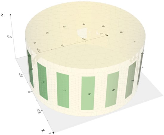
Figure 1.
Simulation of an empty tank for the electrical tomography methods.
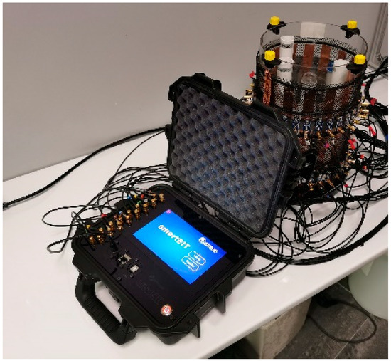
Figure 2.
Electrical impedance tomograph connected to the test tank.
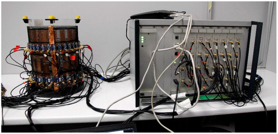
Figure 3.
Electrical capacitance tomograph connected to the test tank.
For reconstruction, the sample was divided into two parts. The learning and testing sets contain 2000 and 3000 cases, respectively (Figure 4).
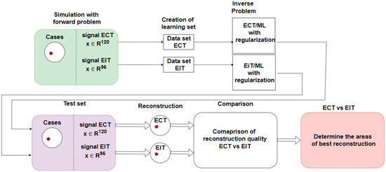
Figure 4.
Simulation and comparison block diagram for electrical tomography methods.
Every 5000 simulated cases are obtained by inserting one to five inclusions into the tank. In each case, the potential difference between each pair of electrodes for EIT and the capacitance measurement for ECT are obtained by solving a forward problem. The simulations were calibrated based on actual measurement data taken with the electrical impedance tomography (Figure 2) and the electrical capacitance tomography (Figure 3).
2.1.1. EIT Measuring Device
The SmartEIT (Figure 2) is an electrical impedance tomography measurement device. This device uses a set of graphite, point-sensing electrodes connected using SMB-electrode coaxial cables. The control and communication system is based on a Raspberry Pi 4 model B single-board minicomputer with a dedicated 7″ LCD touchscreen display with 800 × 480 resolution. The measurement board is equipped with a separate microcontroller from the STM32 family, based on a high-performance ARM® Cortex®-M4 32-bit core, operating at up to 72 MHz, equipped with 256 KB of flash memory, and 32 kB of RAM [14]. A key component of the data acquisition module is a set of built-in high-resolution analog-to-digital converters with software-controlled gain.
In addition, the module has several analog signal conditioning systems, multiplexers switching current and voltage paths, and an isolated dual inverter that boosts the voltage supplying the analog circuits. Since the current source uses the entire range of the supplied voltage, it is possible to obtain a constant current value for objects with relatively high impedance. The input signal is a sinusoidal waveform with a fixed frequency and a constant current value. An additional expansion board is attached to the module via the FPC connector, which enables the electrodes to be connected via coaxial cables. The device is equipped with 16 SMB sockets for connecting the wires and connecting the device to the electrodes.
2.1.2. ECT EVT4
The ECT EVT4 (Figure 3) measurement device [54] is built on high-speed programmable circuits. The multi-mode channel system can use from 4 to 32 channels. Due to the many channels and high signal-to-noise ratio (SNR), it can be used for precise 3D measurements. Each channel has an analog-to-digital converter and multi-gigabit serial transmission for high data throughput, making dynamic imaging possible. In addition, the device utilizes a new capacitance measurement method with its novel single-shot high-voltage (SSHV) circuit.
Together with the distributed control logic architecture, this provides the device with very fast sample conversion times. Furthermore, the tomograph is controlled with proprietary software enabling the user to set measurement parameters, gain ratios, SSHV method timings, and many other settings. Moreover, it can be matched to various capacitive sensors, allowing easy measurements over a wide range along with high speed.
2.2. ElasticNet Method for Image Reconstruction
Reconstructions for both methods were carried out using the elastic net machine-learning method. Elastic net is a regression-based method of parameter estimation in a linear model where, dependent variable, observation matrix independent variable, number of observation, kno. of the dependent variable, parameter vector of the linear model, and error vector. The objective function in a linear model is defined as follows:
Euclidean norm. Classical regression models assume that matrix is revertible (i.e., det). The optimal solution is then
When the dependent variables are excessively correlated with each other, the determinant is close to zero. It disallows the correct estimation of linear model parameters.
Penalization is then used to control the variance of the estimator. It is realized by adding a penalty factor to the objective function:
where, and . This penalization is a linear combination of norms in space and , where, the parameter determines the ratio between the different types of penalization. In addition, the parameter that determines the size of the penalty is defined. In the case when the penalization is carried out in space (LASSO regression); in the case when α = 0 penalization is carried out in space (ridge regression). These models are constructed for each finite element separately.
2.3. Function Comparing Reconstructions
The physics of electrical capacitance tomography measurement is simple due to the lack of alternating current. The measurement is made using the charge-discharge method. Signal energy in ECT decreases with the square distance from the capacitor cover, so the measurement is best near the capacitor cover. Differently, an alternating current source for EIT measurement is applied to the transmitting electrode and the opposite receiving electrode during the measurement. Then, the potential difference (voltage) on the other adjacent electrodes is measured. In this case, the most incredible sensitivity occurs in the vicinity of the electrodes because the energy fluctuation of the electric field is greatest in these areas.
A reconstruction efficiency analysis was performed for both techniques in electrical tomography. In order to determine a more efficient reconstruction, the conductance value in each finite element was first transformed into a capacitance value. This transformation is written in Formula (4) using the function . Then, for each finite element of the interior of the reconstructed object after all reconstructions, the minimum value of the parameter was determined according to equation (2). This parameter takes values in the range
When this parameter takes a value , the EIT reconstruction is considered to be a more efficient reconstruction.
When , ECT reconstruction is considered more effective.
For each finite element , consisting in minimizing the expression
where, -value for finite element for the -th reconstruction, ECT value for the -th reconstruction, coefficients in the elastic net model for the electrical capacitance tomography for the -th finite element EIT value for the -th reconstruction, coefficients in the elastic net model for the electrical impedance tomography for the -th finite element.
3. Results and Discussion
The first step was to train the elastic net model for both electrical tomography methods on 2000 randomly selected cases. Each of the 20,455 finite elements was trained separately. The parameters for which elastic net models were learned are θ = 10−4 and α = 0.3. Example reconstructions for one and three inclusions are shown for both methods. Example reconstructions for one and three inclusions are shown for both methods. Figure 5 shows the reconstruction for one inclusion and Figure 6 shows the impedance differences for EIT. Figure 7 shows the reconstruction for two inclusions and Figure 8 shows the impedance differences for the EIT measurements from Figure 7. Figure 9 shows the reconstruction for two inclusions but with a different inclusion position and Figure 10 shows the impedance differences for the EIT measurements from Figure 9. Figure 11 shows the reconstruction for one inclusion and Figure 12 shows the capacitance differences for ECT. Figure 13 shows the reconstruction for two inclusions, and Figure 14 shows the capacitance differences for the ECT measurements from Figure 13. Figure 15 shows the reconstruction for two inclusions but with a different inclusion position, and Figure 16 shows the capacitance differences for the ECT measurements from Figure 15. In addition, Figure 6, Figure 8, Figure 10, Figure 12, Figure 14, and Figure 16 show impedance differences for EIT, capacitance differences for ECT corresponding to the reference, and the measured values corresponding to the reconstructed case. Such a comparison allows one to see how far the measurements after reconstruction deviate from the reference. For comparison of distance values, the distances of the curves from Figure 6, Figure 8, Figure 10, Figure 12, Figure 14, and Figure 16 are shown in Table 1 and Table 2.
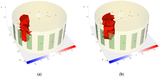
Figure 5.
Comparison of the pattern (a) with reconstruction (b) in the field of view for one inclusion for EIT.
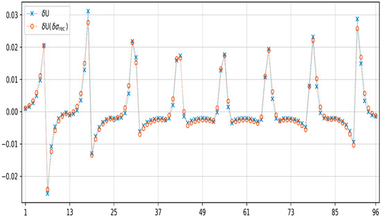
Figure 6.
Comparison of electrode readings for Figure 5.
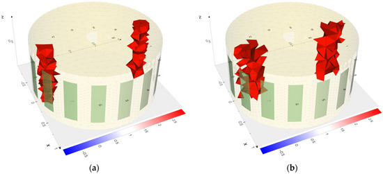
Figure 7.
Comparison of the pattern (a) with reconstruction (b) in the field of view for one inclusion for EIT.
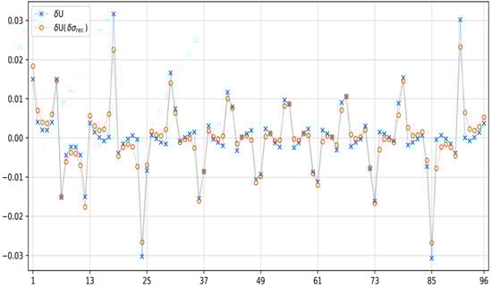
Figure 8.
Comparison of electrode readings for Figure 7.
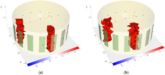
Figure 9.
Comparison of the pattern (a) with reconstruction (b) in the field of view for three inclusions for EIT.
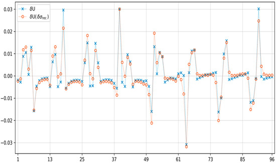
Figure 10.
Comparison of electrode readings for Figure 9.
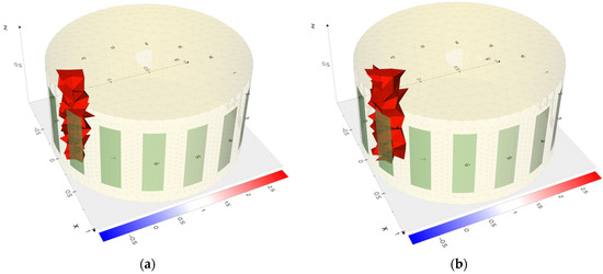
Figure 11.
Comparison of the pattern (a) with the reconstruction (b) in the field of view for one inclusion for ECT.
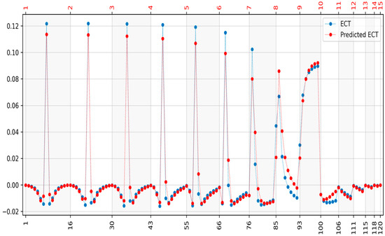
Figure 12.
Comparison of electrode readings for Figure 11.
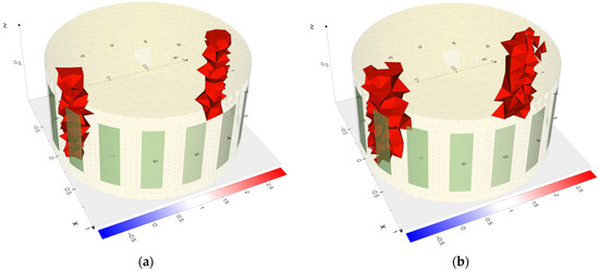
Figure 13.
Comparison of the pattern (a) with the reconstruction (b) in the field of view for three inclusions for ECT.
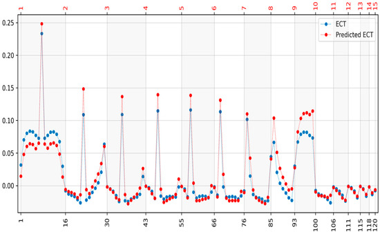
Figure 14.
Comparison of electrode readings for Figure 13.
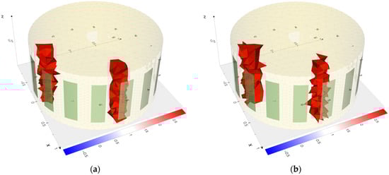
Figure 15.
Comparison of the pattern (a) with the reconstruction (b) in the field of view for three inclusions for ECT.
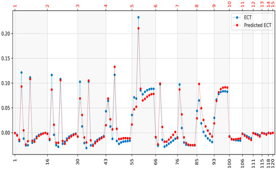
Figure 16.
Comparison of electrode readings for Figure 15.

Table 1.
Distances of original and reconstructed signal for EIT.
Table 2.
Distances of original and reconstructed signal for ECT.
Given the value for the original signal , value for the predicted signal (reconstruction) for each element , the proposed distance measures are:
Root mean square error
Mean absolute error
Mean absolute percentage error
Let I and RI be the original and reconstructed image, respectively. Thus, I(i,j) and RI(i,j) denote the values of (i,j) pixel (1 ≤ I ≤ m, 1 ≤ j ≤ n) in the original and reconstructed image. To assess the reconstruction performance, we use the following measures.
Peak signal-to-noise ratio
Structural similarity index measure
where, μ_I, μ_RI, σ_I^2 and σ_RI^2 denote the pixel sample mean and variance of original I and reconstructed RI images, σ_(I,RI)—covariance of I and RI, c_1, c_2—some constants.
The above coefficients allow us to determine the distance of two signals. RMSE and MAE are similar coefficients. However, MAE, unlike RMSE, treats all distances equally. RMSE, due to the summation of differences of squares between distances, magnifies large differences between values. The MAPE coefficient expresses in percentage terms the relative differences to the value of the original signal.
3.1. Reconstruction EIT
For EIT reconstructions, individual inclusions, especially those close to the electrodes (Figure 5), are reconstructed better than those in the center (Figure 7). In the case of a larger number of inclusions when the inclusions are distant from each other, the obtained reconstructions of individual inclusions are clear. In the case of a larger number of inclusions placed close together, the reconstructions of the individual objects merge into a single area (Figure 9).
3.2. Reconstruction ECT
For reconstructions obtained with electrical capacitance tomography for multiple inclusions closer to the center of the study area, they are better reconstructed than with electrical impedance tomography. In contrast, the ECT method better reconstructs objects closer to the electrodes for single inclusions. Electrical capacitance tomography has more problems recognizing object boundaries closer to the center of the object’s interior.
Based on the results, reconstruction efficiency parameters were calculated for each finite element according to Equation (2). Figure 17 shows the areas where one of the reconstruction methods is more effective. In the graph, the red color indicates areas better reconstructed by the ECT method, and the cream color indicates areas better reconstructed by the EIT method.
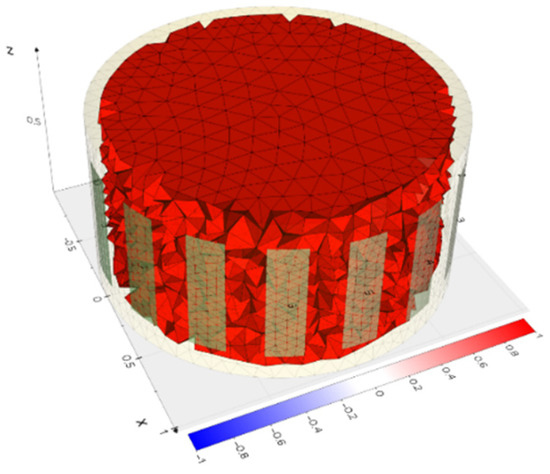
Figure 17.
Areas of reconstruction highlight the effectiveness of methods.
The results show that the area closer to the center of the reservoir is better reconstructed by electrical capacitance tomography, while the edges of the reservoir are more efficiently reconstructed by electrical impedance tomography. Furthermore, the percentage of finite elements with better efficiency of ECT compared to EIT is 65% to 35%.
The simulations show that electrical impedance tomography gives better reconstruction quality near the reservoir edge than electrical capacitance tomography. Theoretically, it is because both methods better reconstruct objects closer to the edge of the tank. However, the fluctuation of signal energy closer to the edge of the tomography is more significant for electrical impedance tomography than electrical capacitance tomography, resulting in better reconstruction quality. In contrast, the situation is reversed for the ECT method.
3.3. Real Measurements
Real-world tests were conducted to verify the results of the simulation studies. Block diagram of the measurement method is presented in Figure 18. First, phantoms were placed in a tank to which electrodes were connected. Then, measurements were taken as in Figure 19a, Figure 20a, Figure 21a, Figure 22a andFigure 23a with EVT4 (Figure 3) and SmartEIT (Figure 2) devices. Next, reconstructions were made using the elastic net method with models learned from simulation data.
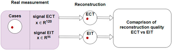
Figure 18.
Block diagram of the measurement method for ECT and EIT.
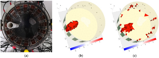
Figure 19.
(a) Placing the measurement phantom in the tank, (b) image reconstruction based on EIT and (c) ECT tomography measurements.
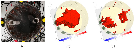
Figure 20.
(a) Placement of measurement phantoms in the tank, (b) image reconstruction based on EIT, and (c) ECT tomography measurements.
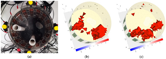
Figure 21.
(a) Placement of measurement phantoms in the tank, (b) image reconstruction based on EIT and (c) ECT tomography measurements.
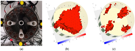
Figure 22.
(a) Placement of measurement phantoms in the tank, (b) image reconstruction based on EIT, and (c) ECT tomography measurements.
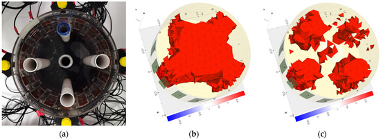
Figure 23.
(a) Placement of measurement phantoms in the tank, (b) image reconstruction based on EIT, and (c) ECT tomography measurements.
The results of the actual measurements confirm the conclusions obtained by comparing the reconstructions with the simulations. For example, in Figure 22a,b and Figure 23a,b, it can be observed that the centers of the reconstructed areas are blended for electrical impedance tomography. In contrast, for electrical capacitance tomography, the inclusions within the center of the reservoir are reconstructed as distinct inclusion. Thus, inclusions in that area are better reconstructed by the ECT method than by EIT.
The results obtained with the paper were compared to those found in the literature. In the paper [59], the authors got the best results with the autoencoder. The error range was from 0.5976 for one element to 0.6601 for five elements.
In another of the papers [58], the authors use correlation coefficient (CC) and structural similarity (SS) as evaluation criteria, and the results are presented for RBFNN and HPSO-RBFNN networks. Better results were obtained for the RBFNN method and, depending on the number of elements, are 0.086 for SS two objects and 0.643 for CC, and, similarly for three objects, 0.047 and 0.365, respectively.
In the different paper [65], the authors obtained very good results for the LeNet solution and an absolute error ranging from 0.039 to 0.057.
Comparing this further with the results of paper [67] where the authors presented their achievements for the TSDL method, they obtained an RMSE error of 8.7 ± 0.8 for one group of images and 9.2 ± 1.43 for the other group of images containing lung phantoms.
4. Conclusions
This paper presents the effectiveness of reconstruction by different methods in electrical tomography. The research was conducted on 5000 simulated inclusion cases. In the first step, the reconstruction algorithm was taught on a sample of randomly selected 2000 patterns using elastic net. Then, the remaining 3000 cases were reconstructed using the learned algorithm. The function defined by equation (2) was used in the next step. Finally, the areas that most efficiently reconstruct images from the measurement data were determined.
During training, the model was presented with cases with up to two inclusions. During the validation stage on actual measurement data, the model was effective for cases with more than two inclusions. However, for measurements with more than three inclusions, the predictions of central inclusions are worse than in other cases. This result is expected because inclusions near the edge of the tank “shield” the object and distort the electric field in the center of the tank, resulting in less information during measurement. In the next step, individual cases were reconstructed based on real measurements. Finally, based on the presented analysis, the results of the simulation studies were validated, confirming the results obtained earlier for the simulated data.
The results show that electrical capacitance tomography is better for areas closer to the center of the tank, where efficiency is about 65% of all finite elements. On the other hand, electrical impedance tomography gives better results for objects closer to the electrodes, which includes about 35% of all grid elements. These findings are directly related to the energy fluctuations for each method in different areas of the tank. Larger fluctuations in signal energy yield better reconstruction quality. For the EIT method, larger fluctuations in electric field energy than for the ECT method will occur at the edge of the reservoir. Similarly, in the center of the field of view, we will get larger fluctuations of electric field energy for capacitive electrical tomography; thus, this method gives the best results.
Author Contributions
Development of the concept of algorithms and implementation of the image reconstruction in electrical impedance tomography and electrical capacitance tomography, E.K., D.W. and B.P.; development of the system concept, measurement methodology, and supervision, T.R.; preparation of measurements, development of research methodology, preparation of measurement documentation K.K. and M.G.; literature review, formal analysis, general review, and editing of the manuscript, B.P., D.W., T.R. and K.K. All authors have read and agreed to the published version of the manuscript.
Funding
This research received no external funding.
Institutional Review Board Statement
Not applicable.
Informed Consent Statement
Not applicable.
Data Availability Statement
Not applicable.
Conflicts of Interest
The authors declare no conflict of interest.
References
- Rymarczyk, T.; Kłosowski, G. Innovative methods of neural reconstruction for tomographic images in maintenance of tank industrial reactors. Eksploat. Niezawodn. Maint. Reliab. 2019, 21, 261–267. [Google Scholar] [CrossRef]
- Wang, F.; Marashdeh, Q.; Fan, L.S.; Warsito, W. Electrical Capacitance Volume Tomography: Design and Applications. Sensors 2010, 10, 1890–1917. [Google Scholar] [CrossRef] [PubMed]
- Garbaa, H.; Jackowska-Strumiłło, L.; Grudzień, K.; Romanowski, A. Application of Electrical Capacitance Tomography and Artificial Neural Networks to Rapid Estimation of Cylindrical Shape Parameters of Industrial Flow Structure. Arch. Electr. Eng. 2016, 65, 657–669. [Google Scholar] [CrossRef]
- Rymarczyk, T.; Niderla, K.; Kozłowski, E.; Król, K.; Wyrwisz, J.M.; Skrzypek-Ahmed, S.; Gołąbek, P. Logistic Regression with Wave Preprocessing to Solve Inverse Problem in Industrial Tomography for Technological Process Control. Energies 2021, 14, 8116. [Google Scholar] [CrossRef]
- Rymarczyk, T.; Kłosowski, G.; Kozłowski, E. A Non-Destructive System Based on Electrical Tomography and Machine Learning to Analyze the Moisture of Buildings. Sensors 2018, 18, 2285. [Google Scholar] [CrossRef]
- Berowski, P.; Filipowicz, S.F.; Sikora, J.; Wójtowicz, S. Determining location of moisture area of the wall by 3D electrical impedance tomography. In Proceedings of the 4th World Congress in Industrial Process Tomography, Aizu, Japan, 5–8 September 2005; pp. 214–219. [Google Scholar]
- Kłosowski, G.; Rymarczyk, T.; Gola, A. Increasing the Reliability of Flood Embankments with Neural Imaging Method. Appl. Sci. 2018, 8, 1457. [Google Scholar] [CrossRef]
- Rymarczyk, T.; Król, K.; Kozłowski, E.; Wołowiec, T.; Cholewa-Wiktor, M.; Bednarczuk, P. Application of Electrical Tomography Imaging Using Machine Learning Methods for the Monitoring of Flood Embankments Leaks. Energies 2021, 14, 8081. [Google Scholar] [CrossRef]
- Mikulka, J. GPU-Accelerated Reconstruction of T2 Maps in Magnetic Resonance Imaging. Meas. Sci. Rev. 2015, 4, 210–218. [Google Scholar] [CrossRef]
- Przysucha, B.; Rymarczyk, T.; Wójcik, D.; Woś, M.; Vejar, A. Improving the Dependability of the ECG Signal for Classification of Heart Diseases. In Proceedings of the 50th Annual IEEE-IFIP International Conference on Dependable Systems and Networks-Supplemental Volume (DSN-S), Valencia, Spain, 2–29 July 2020; pp. 63–64. [Google Scholar] [CrossRef]
- Rymarczyk, T.; Kozłowski, E.; Tchórzewski, P.; Kłosowski, G.; Adamkiewicz, P. Applying the logistic regression in electrical impedance tomography to analyze conductivity of the examined objects. J. Appl. Electromagn. Mech. 2020, 64, 235–252. [Google Scholar] [CrossRef]
- Rymarczyk, T.; Kozłowski, E.; Kłosowski, G. Electrical impedance tomography in 3D flood embankments testing–elastic net approach. Transactions Inst. Meas. Control. 2019, 42, 680–690. [Google Scholar] [CrossRef]
- Rymarczyk, T.; Szumowski, J.; Adamkiewicz, P.; Duda, K.; Sikora, J. ECT measurement system with optical detection for quality control of flow process. Przegląd Elektrotechniczny 2016, 92, 157–160. [Google Scholar] [CrossRef]
- Rymarczyk, T.; Bożek, P.; Oleszek, M.; Niderla, K.; Adamkiewicz, P. Construction of the SmartEIT tomograph based on electrical impedance tomography. Przegląd Elektrotechniczny 2020, 1, 44–47. [Google Scholar] [CrossRef]
- Rymarczyk, T.; Sikora, J.; Adamkiewicz, P.; Niderla, K.; Tchórzewski, P. Analysis and Monitoring of Flood Embankments Through Image Reconstruction Based on Electrical Impedance Tomography. In Proceedings of the 19th International Symposium on Electromagnetic Fields in Mechatronics, Electrical and Electronic Engineering (ISEF), Nancy, France, 29–31 August 2019; pp. 1–2. [Google Scholar] [CrossRef]
- Herman, G.T. Image Reconstruction from Projections: The Fundamentals of Computerized Tomography; Academic Press: New York, NY, USA, 1980. [Google Scholar]
- Kak, A.C.; Slaney, M. Principles of Computerized Tomographic Imaging; IEEE Press: New York, NY, USA, 1999. [Google Scholar]
- Beck, M.S.; Williams, R.A. Process tomography: A European innovation and its applications. Meas. Sci. Technol. 1996, 7, 215–224. [Google Scholar] [CrossRef]
- Banasiak, R.; Wajman, R.; Jaworski, T.; Fiderek, P.; Fidos, H.; Nowakowski, J.; Sankowski, D. Study on two-phase flow regime visualization and identification using 3D electrical capacitance tomography and fuzzy-logic classification. Int. J. Multiph. Flow 2014, 58, 1–14. [Google Scholar] [CrossRef]
- Dusek, J.; Kikulka, J. Measurement-Based Domain Parameter Optimization in Electrical Impedance Tomography Imaging. Sensors 2021, 21, 2507. [Google Scholar] [CrossRef]
- Kryszyn, J.; Smolik, W. Toolbox for 3D modelling and image reconstruction in electrical capacitance tomography. Inform. Control. Meas. Econ. Environ. Prot. 2017, 7, 137–145. [Google Scholar] [CrossRef]
- Kryszyn, J.; Wanta, D.M.; Smolik, W.T. Gain Adjustment for Signal-to-Noise Ratio Improvement in Electrical Capacitance Tomography System EVT4. IEEE Sens. J. 2017, 17, 8107–8116. [Google Scholar] [CrossRef]
- Majchrowicz, M.; Kapusta, P.; Jackowska-Strumiłło, L.; Sankowski, D. Acceleration of image reconstruction process in the electrical capacitance tomography 3D in heterogeneous, multi-GPU system. Inform. Control. Meas. Econ. Environ. Prot. 2017, 7, 37–41. [Google Scholar] [CrossRef]
- Wajman, R.; Fiderek, P.; Fidos, H.; Jaworski, T.; Nowakowski, J.; Sankowski, D.; Banasiak, R. Metrological evaluation of a 3D electrical capacitance tomography measurement system for two-phase flow fraction determination. Meas. Sci. Technol. 2013, 24, 065302. [Google Scholar] [CrossRef]
- Duraj, A.; Korzeniewska, E.; Krawczyk, A. Classification algorithms to identify changes in resistance. Przegląd Elektrotechniczny 2015, 1, 82–84. [Google Scholar] [CrossRef]
- Szczęsny, A.; Korzeniewska, E. Selection of the method for the earthing resistance measurement. Przegląd Elektrotechniczny 2018, 94, 178–181. [Google Scholar] [CrossRef]
- Morigi, M.P.; Albertin, F. X-ray Digital Radiography and Computed Tomography. J. Imaging 2022, 8, 119. [Google Scholar] [CrossRef] [PubMed]
- Majerek, D.; Rymarczyk, T.; Wójcik, D.; Kozłowski, E.; Rzemieniak, M.; Gudowski, J.; Gauda, K. Machine Learning and Deterministic Approach to the Reflective Ultrasound Tomography. Energies 2021, 14, 7549. [Google Scholar] [CrossRef]
- Zywica, A.R.; Ziolkowski, M.; Gratkowski, S. Detailed Analytical Approach to Solve the Magnetoacoustic Tomography with Magnetic Induction (MAT-MI) Problem for Three-Layer Objects. Energies 2020, 13, 6515. [Google Scholar] [CrossRef]
- Xi, Y.; Qiao, Z.; Wang, W.; Niu, L. Study of CT image reconstruction algorithm based on high order total variation. Optik 2020, 204, 163814. [Google Scholar] [CrossRef]
- Bangti, J.; Maass, P. An Analysis of Electrical Impedance Tomography with Applications to Tikhonov Regularization. ESAIM COCV 2012, 18, 1027–1048. [Google Scholar] [CrossRef]
- Kłosowski, G.; Hoła, A.; Rymarczyk, T.; Skowron, Ł.; Wołowiec, T.; Kowalski, M. The Concept of Using LSTM to Detect Moisture in Brick Walls by Means of Electrical Impedance Tomography. Energies 2021, 14, 7617. [Google Scholar] [CrossRef]
- Rymarczyk, T.; Kłosowski, G. The use of elastic net and neural networks in industrial process tomography. Przegląd Elektrotechniczny 2019, 1, 61–64. [Google Scholar] [CrossRef]
- Rymarczyk, T.; Kłosowski, G.; Hoła, A.; Sikora, J.; Wołowiec, T.; Tchórzewski, P.; Skowron, S. Comparison of Machine Learning Methods in Electrical Tomography for Detecting Moisture in Building Walls. Energies 2021, 14, 2777. [Google Scholar] [CrossRef]
- Kłosowski, G.; Rymarczyk, T.; Niderla, K.; Rzemieniak, M.; Dmowski, A.; Maj, M. Comparison of Machine Learning Methods for Image Reconstruction Using the LSTM Classifier in Industrial Electrical Tomography. Energies 2021, 14, 7269. [Google Scholar] [CrossRef]
- Serte, S.; Demirel, H. Deep learning for diagnosis of COVID-19 using 3D CT scans. Comput. Biol. Med. 2021, 132, 104306. [Google Scholar] [CrossRef]
- Zhang, J.; Yan, Y.; Ni, H. Lung detection and severity prediction of pneumonia patients based on COVID-19 DET-PRE network. Expert Rev. Med. Devices 2022, 19, 97–106. [Google Scholar] [CrossRef]
- Zhang, B.; He, X.; Ouyang, F.; Gu, D.; Dong, Y.; Zhang, L.; Mo, X.; Huang, W.; Tian, J.; Zhang, S. Radiomic machine-learning classifiers for prognostic biomarkers of advanced nasopharyngeal carcinoma. Cancer Lett. 2017, 403, 21–27. [Google Scholar] [CrossRef]
- Huang, S.; Yang, J.; Fong, S.; Zhao, Q. Artificial intelligence in cancer diagnosis and prognosis: Opportunities and challenges. Cancer Lett. 2020, 471, 61–71. [Google Scholar] [CrossRef]
- Bahramiabarghouei, H.; Porter, E.; Santorelli, A.; Gosselin, B.; Popović, M.; Rusch, L.A. Flexible 16 antenna array for microwave breast cancer detection. IEEE Trans. Biomed. Eng. 2015, 62, 2516–2525. [Google Scholar] [CrossRef]
- O’Loughlin, D.; O’Halloran, M.; Moloney, B.M.; Glavin, M.; Jones, E.; Elahi, M.A. Microwave breast imaging: Clinical advances and remaining challenges. IEEE Trans. Biomed. Eng. 2018, 65, 2580–2590. [Google Scholar] [CrossRef]
- Mojabi, P.; Vetri, J.L. Development of an ultrasound tomography system: Preliminary results. J. Acoust. Soc. Am. 2016, 140, 3419. [Google Scholar] [CrossRef]
- Wiskin, J.; Malik, B.; Borup, D.; Pirshafiey, N.; John Klock, J. Full wave 3D inverse scattering transmission ultrasound tomography in the presence of high contrast. Sci. Rep. 2020, 10, 20166. [Google Scholar] [CrossRef]
- Przysucha, B.; Rymarczyk, T.; Wójcik, D. Classification of heart rhythm disturbances based on BSPM measurements. J. Phys. Conf. Ser. 2022, 2408, 012003. [Google Scholar] [CrossRef]
- Rymarczyk, T.; Nita, P.; Vejar, A.; Woś, M.; Oleszek, M.; Adamkiewicz, P. Architecture of a mobile system for the analysis of biomedical signals based on electrical tomography. In Proceedings of the 2018 Applications of Electromagnetics in Modern Techniques and Medicine (PTZE), Racławice, Poland, 9–12 September 2018; pp. 236–239. [Google Scholar] [CrossRef]
- Yapici, M.K.; Alkhidir, T.E. Intelligent medical garments with graphene-functionalized smart-cloth ecg sensors. Sensors 2017, 17, 875. [Google Scholar] [CrossRef]
- Zhu, H.; Sun, J.; Xu, L.; Tian, W.; Sun, S. Permittivity Reconstruction in Electrical Capacitance Tomography Based on Visual Representation of Deep Neural Network. IEEE Sens. J. 2020, 20, 4803–4815. [Google Scholar] [CrossRef]
- Deabes, W.K.; Khayyat, M.J. Image Reconstruction in Electrical Capacitance Tomography Based on Deep Neural Networks. IEEE Sens. J. 2021, 21, 25818–25830. [Google Scholar] [CrossRef]
- Deabes, W.; Sheta, A.; Braik, M. ECT-LSTM-RNN: An Electrical Capacitance Tomography Model-Based Long Short-Term Memory Recurrent Neural Networks for Conductive Materials. IEEE Access 2021, 9, 76325–76339. [Google Scholar] [CrossRef]
- Kłosowski, G.; Rymarczyk, T. Monitoring of flood embankments through EIT machine ensemble learning. Int. J. Appl. Electromagn. Mech. 2022, 69, 211–220. [Google Scholar] [CrossRef]
- Salama, A.; Malekmohammadi, A.; Mohanna, S.; Rajkumar, R. A Multitasking Electrical Impedance Tomography System Using Titanium Alloy Electrode. Int. J. Biomed. Imaging 2017, 2017, 3589324. [Google Scholar] [CrossRef]
- Rymarczyk, T.; Oleszek, M.; Szumowski, J.; Tchórzewski, P.; Adamkiewicz, P.; Sikora, J. A hybrid tomography for assessing the moisture level of walls and building condition. Przegląd Elektrotechniczny 2019, 95, 100–103. [Google Scholar] [CrossRef]
- Saied, I.; Meribout, M. Electronic hardware design of electrical capacitance tomography systems. Philos. Trans. R. Soc. A 2016, 374, 20150331. [Google Scholar] [CrossRef]
- Kryszyn, J.; Wróblewski, P.; Stosio, M.; Wanta, D.; Olszewski, T.; Smolik, W.T. Architecture of EVT4 data acquisition system for electrical capacitance tomography. Measurement 2017, 101, 28–39. [Google Scholar] [CrossRef]
- Sun, J.; Yang, W. A dual-modality electrical tomography sensor for measurement of gas–oil–water stratified flows. Measurement 2015, 66, 150–160. [Google Scholar] [CrossRef]
- Kłosowski, G.; Rymarczyk, T.; Tchórzewski, P.; Bednarczuk, P.; Kowalski, M. Neural Hybrid Tomography for Monitoring industrial reactors. Przegląd Elektrotechniczny 2020, 97, 190–193. [Google Scholar] [CrossRef]
- Leijsen, R.; Brink, W.; van den Berg, C.; Webb, A.; Remis, R. Electrical Properties Tomography: A methodological review. Diagnostics 2021, 11, 176. [Google Scholar] [CrossRef] [PubMed]
- Wang, R.C.; Gao, Y.; Wang, G.J.; Li, Q.P.; Wang, Q.; Wang, H.G. Investigation of complex permittivity/conductivity distribution by electrical tomography. IOP Conf. Ser. Earth Environ. Sci. 2021, 701, 012038. [Google Scholar] [CrossRef]
- Wu, X.J.; Xu, M.D.; Li, C.D.; Ju, C.; Zhao, Q.; Liu, S.X. Research on image reconstruction algorithms based on autoencoder neural network of Restricted Boltzmann Machine (RBM). Flow Meas. Instrum. 2021, 80, 102009. [Google Scholar] [CrossRef]
- Zhang, M.; Ma, Y.; Huang, N. Survey of EIT Image Reconstruction Algorithms. J. Shanghai Jiaotong Univ. 2022, 27, 211–218. [Google Scholar] [CrossRef]
- Kłosowski, G.; Maj, M.; Oleszek, M. Comparison of CNN and LSTM algorithms for solving the EIT inverse problem. Przegląd Elektrotechniczny 2023, 99, 230–233. [Google Scholar] [CrossRef]
- Borsoi, R.A.; Aya, J.C.C.; Costa, G.H.; Bermudez, J.C.M. Super-resolution reconstruction of electrical impedance tomography images. Comput. Electr. Eng. 2018, 69, 1–13. [Google Scholar] [CrossRef]
- Wang, H.; Liu, K.; Wu, Y.; Wang, S.; Zhang, Z.; Li, F.; Yao, J. Image Reconstruction for Electrical Impedance Tomography Using Radial Basis Function Neural Network Based on Hybrid Particle Swarm Optimization Algorithm. IEEE Sens. J. 2021, 21, 1926–1934. [Google Scholar] [CrossRef]
- Gomes, J.C.; Pereira, J.M.S.; de Santana, M.A.; da Silva, W.W.A.; de Souza, R.E.; dos Santos, W.P. Chapter eight-Electrical impedance tomography image reconstruction based on autoencoders and extreme learning machines. In Deep Learning for Data Analytics; Das, H., Pradhan, C., Dey, N., Eds.; Academic Press: Cambridge, MA, USA, 2020; pp. 155–171. [Google Scholar] [CrossRef]
- Bianchessi, A.; Akamine, R.H.; Duran, G.C.; Tanabi, N.; Sato, A.K.; Martins, T.C.; Tsuzuki, M.S.G. Electrical Impedance Tomography Image Reconstruction Based on Neural Networks. IFAC-Pap. 2020, 53, 15946–15951. [Google Scholar] [CrossRef]
- Rymarczyk, T.; Kłosowski, G.; Hoła, A.; Sikora, J.; Tchórzewski, P.; Skowron, Ł. Optimizing the use of Machine learning algorithms in electrical tomography of building Walls: Pixel oriented ensemble approach. Measurement 2022, 188, 110581. [Google Scholar] [CrossRef]
- Ren, S.; Sun, K.; Tan, C.; Dong, F. A Two-Stage Deep Learning Method for Robust Shape Reconstruction With Electrical Impedance Tomography. IEEE Trans. Instrum. Meas. 2020, 69, 4887–4897. [Google Scholar] [CrossRef]
Disclaimer/Publisher’s Note: The statements, opinions and data contained in all publications are solely those of the individual author(s) and contributor(s) and not of MDPI and/or the editor(s). MDPI and/or the editor(s) disclaim responsibility for any injury to people or property resulting from any ideas, methods, instructions or products referred to in the content. |
© 2023 by the authors. Licensee MDPI, Basel, Switzerland. This article is an open access article distributed under the terms and conditions of the Creative Commons Attribution (CC BY) license (https://creativecommons.org/licenses/by/4.0/).