

A Hybrid Analytical Model for the Electromagnetic Analysis of Surface-Mounted Permanent-Magnet Machines Considering Stator Saturation


Abstract
1. Introduction
1.1. Numerical Methods
1.2. Analytical Methods
1.3. Hybrid Methods
1.4. This Article
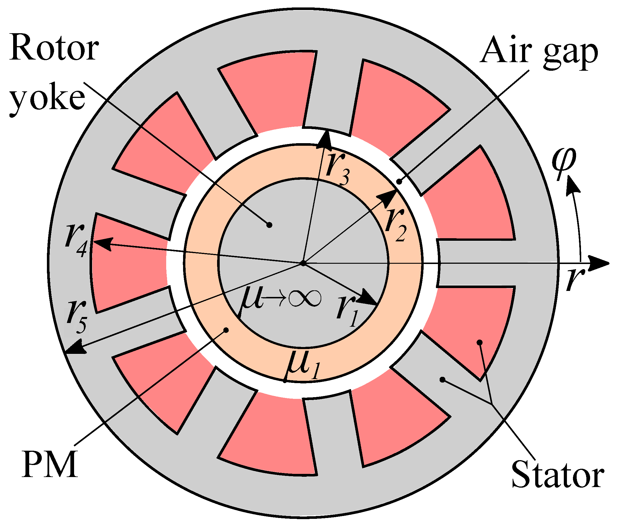
2. Hybrid Model
2.1. Analytical Model in PMs and Air Gap
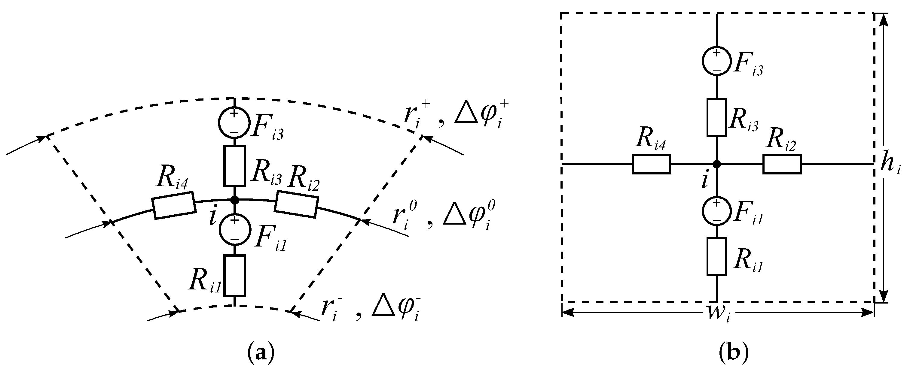
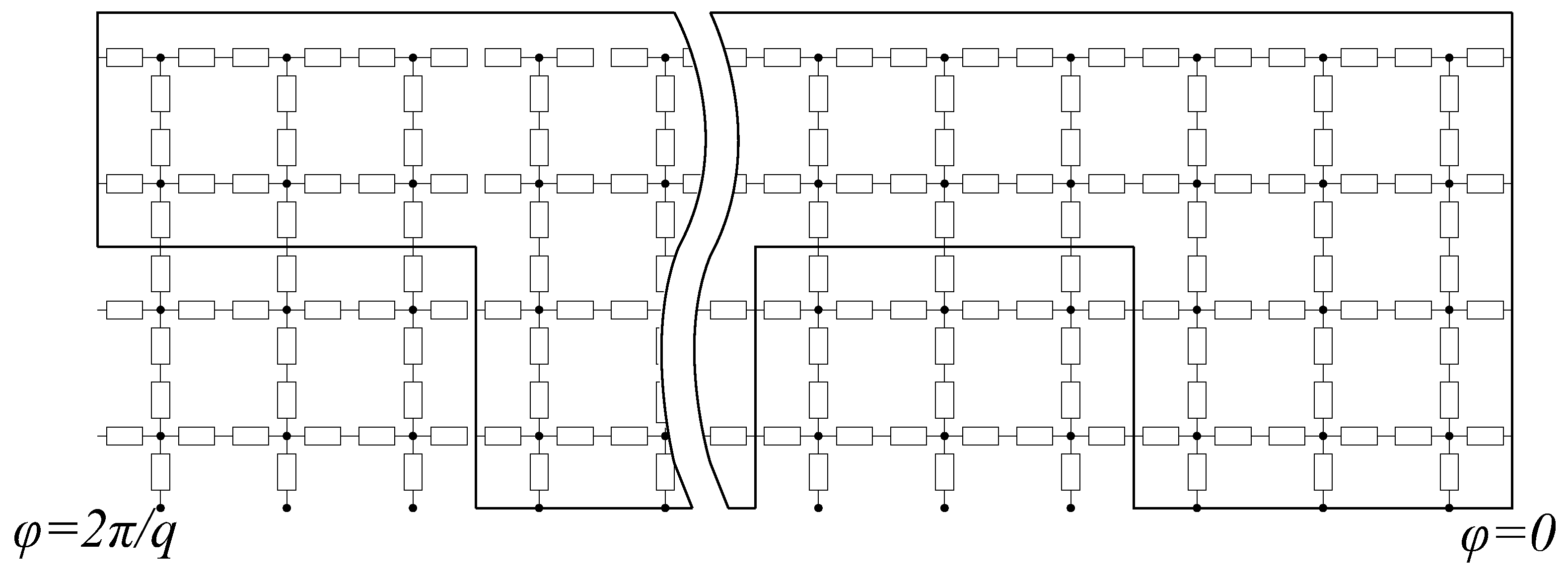
2.2. Reluctance Network Model in Stator
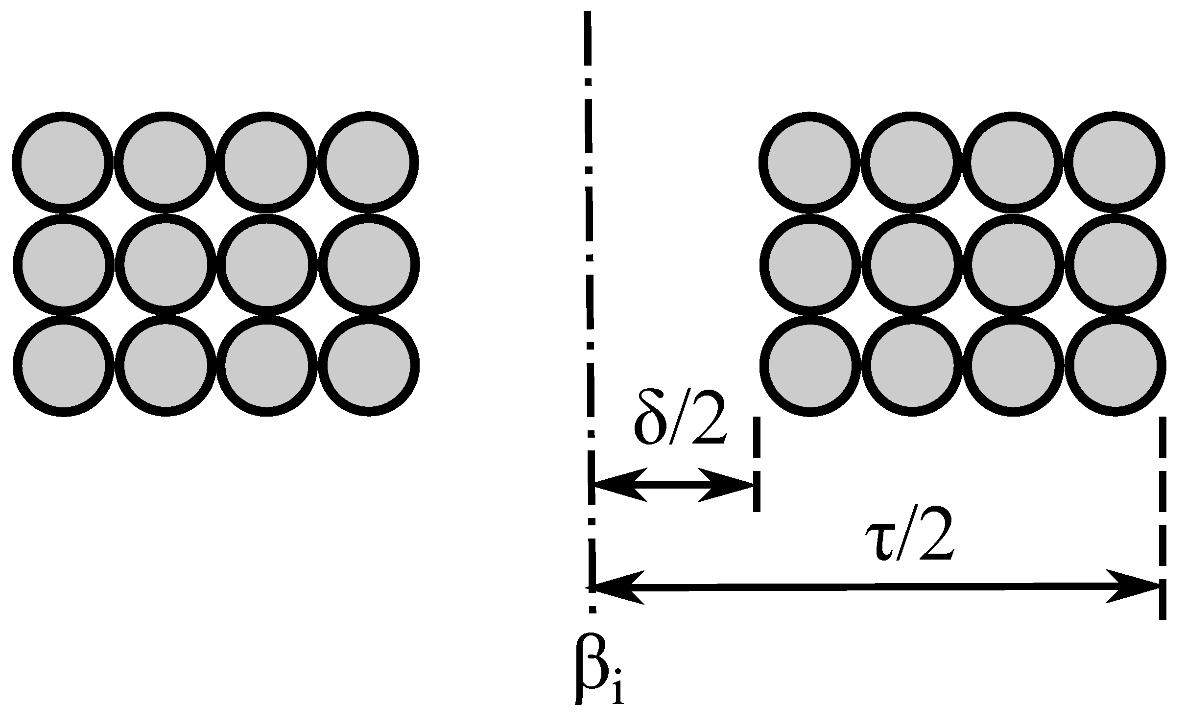
2.2.1. Calculation of Reluctances
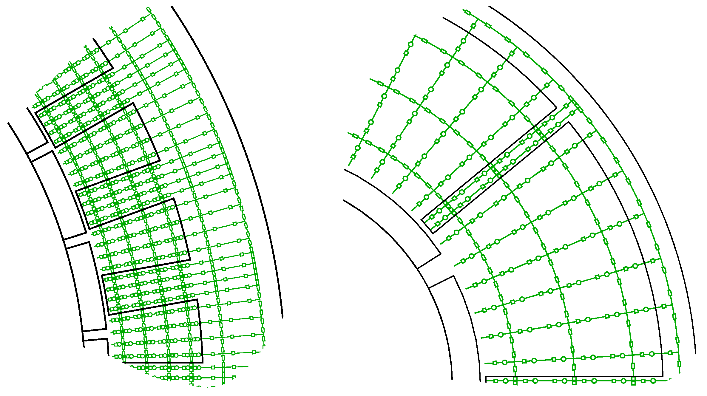
2.2.2. Arrangement of Mesh Elements
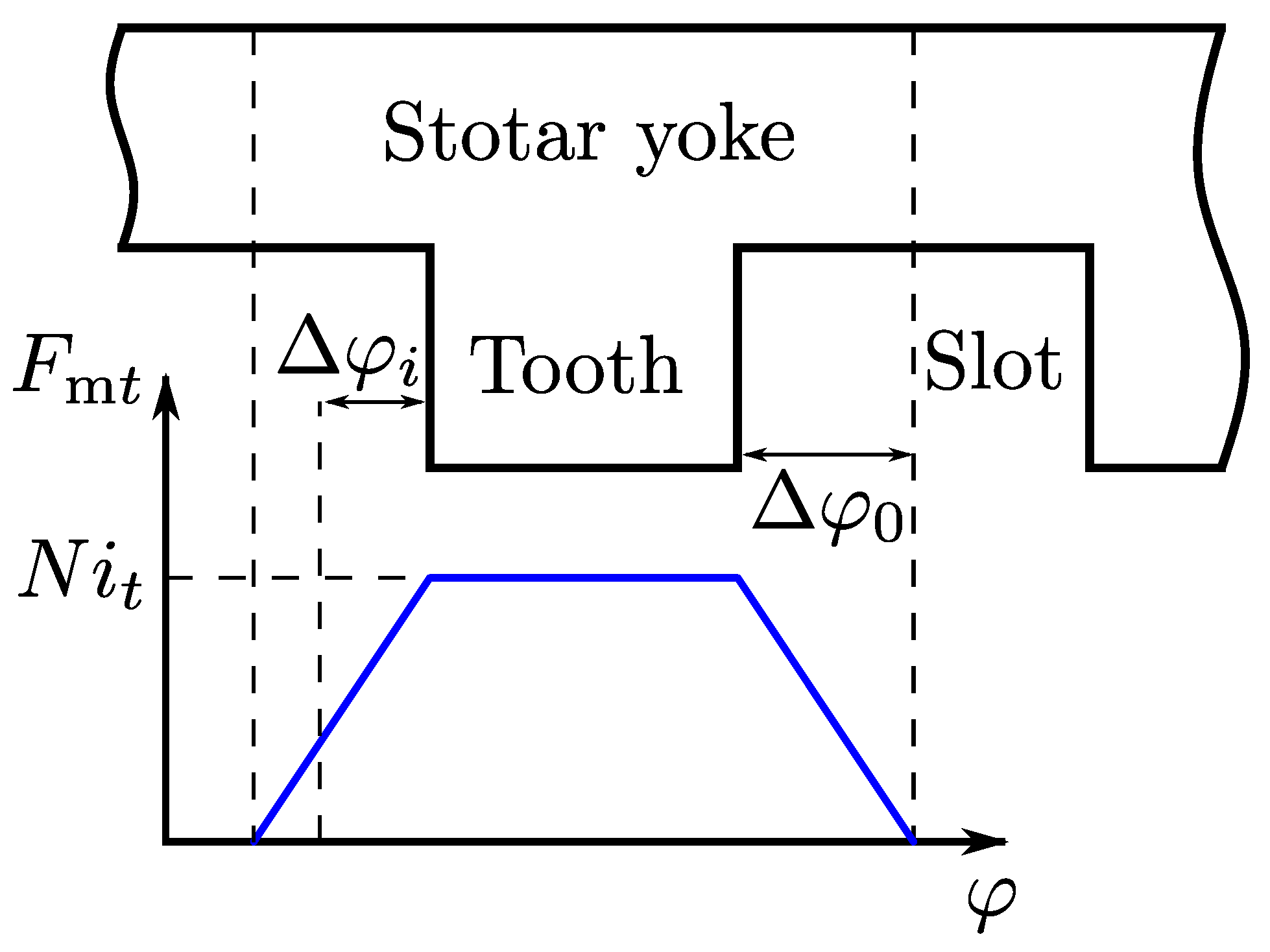
2.2.3. Calculation of Magnetic Source
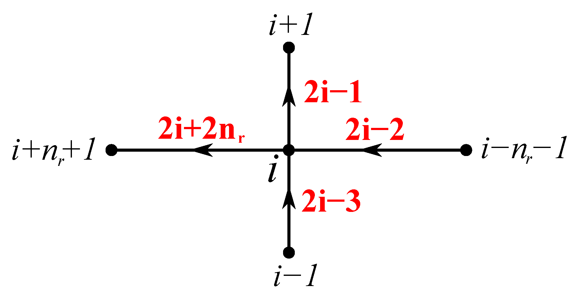
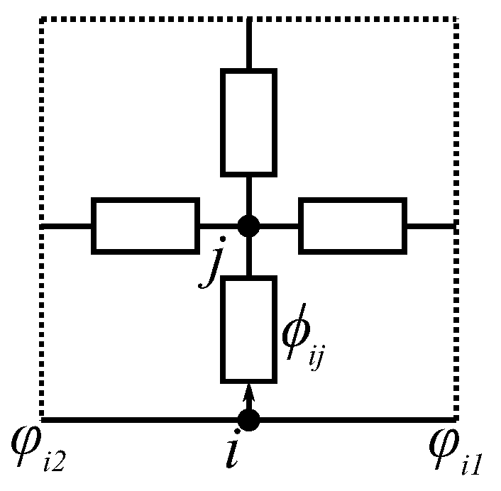
2.2.4. Nodal Potential Equation
2.3. Coupling of the Two Models
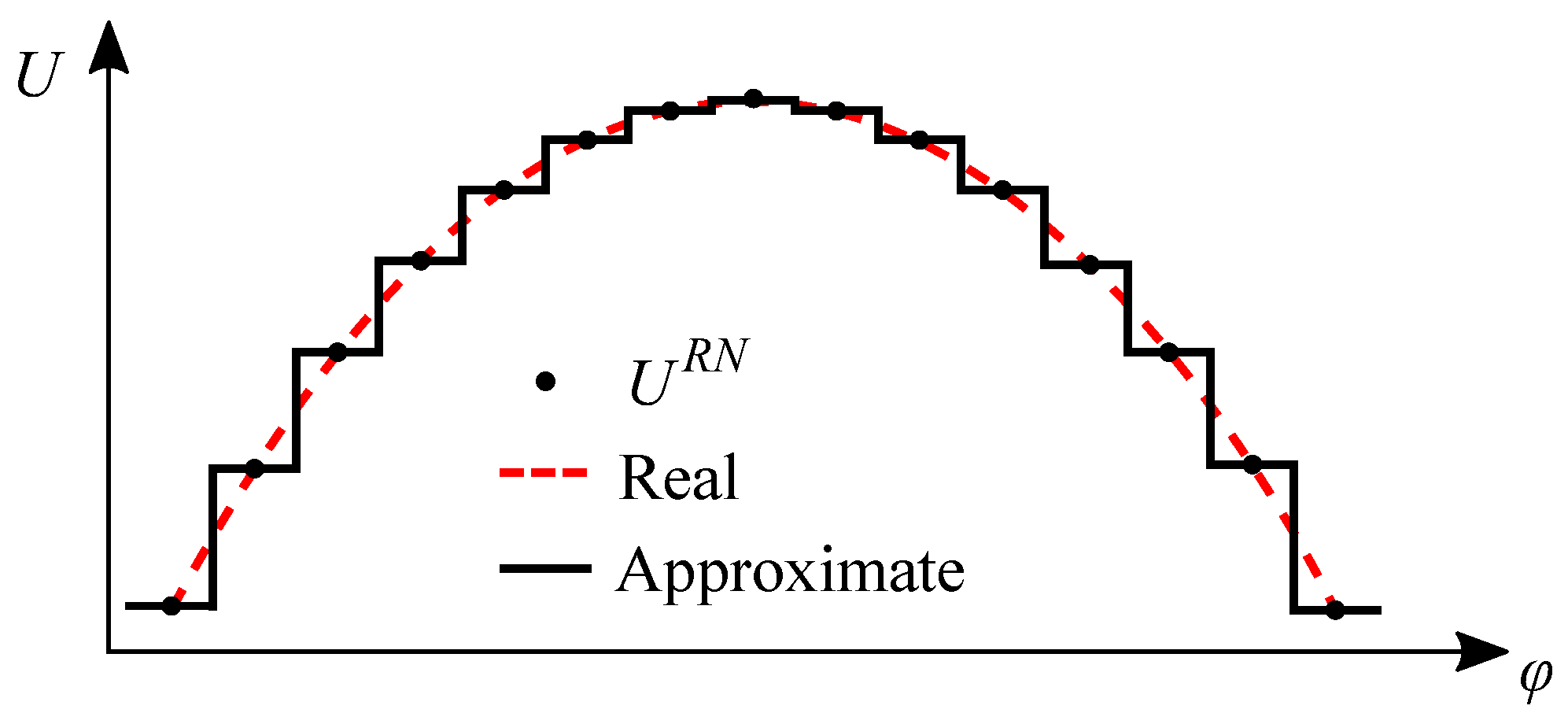
2.3.1. Harmonic Form of Nodal Magnetic Potential
2.3.2. Boundary Conditions at
2.4. Matrix Form
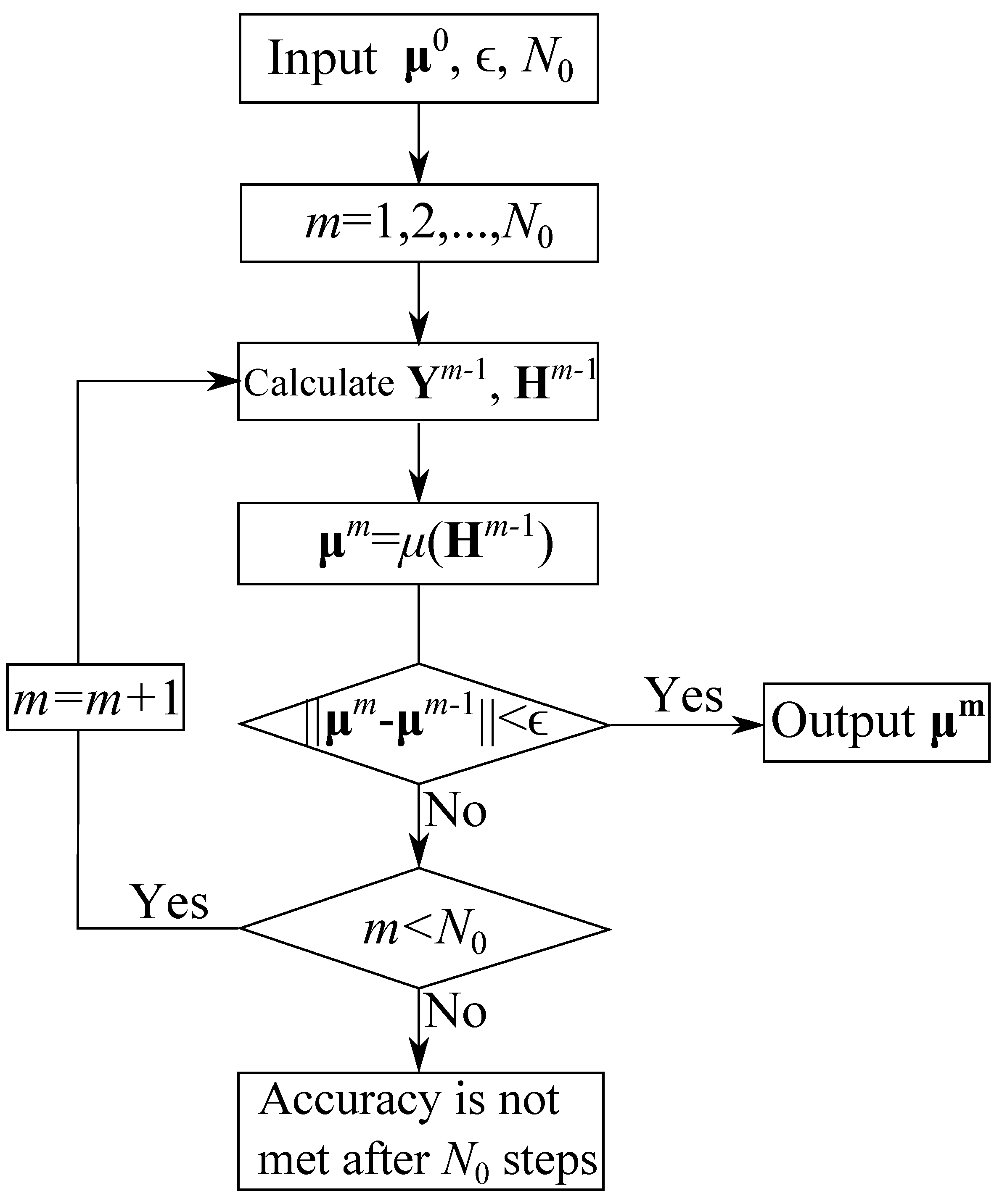
2.5. Nonlinear Analysis
2.6. Post-Processing
3. Validation
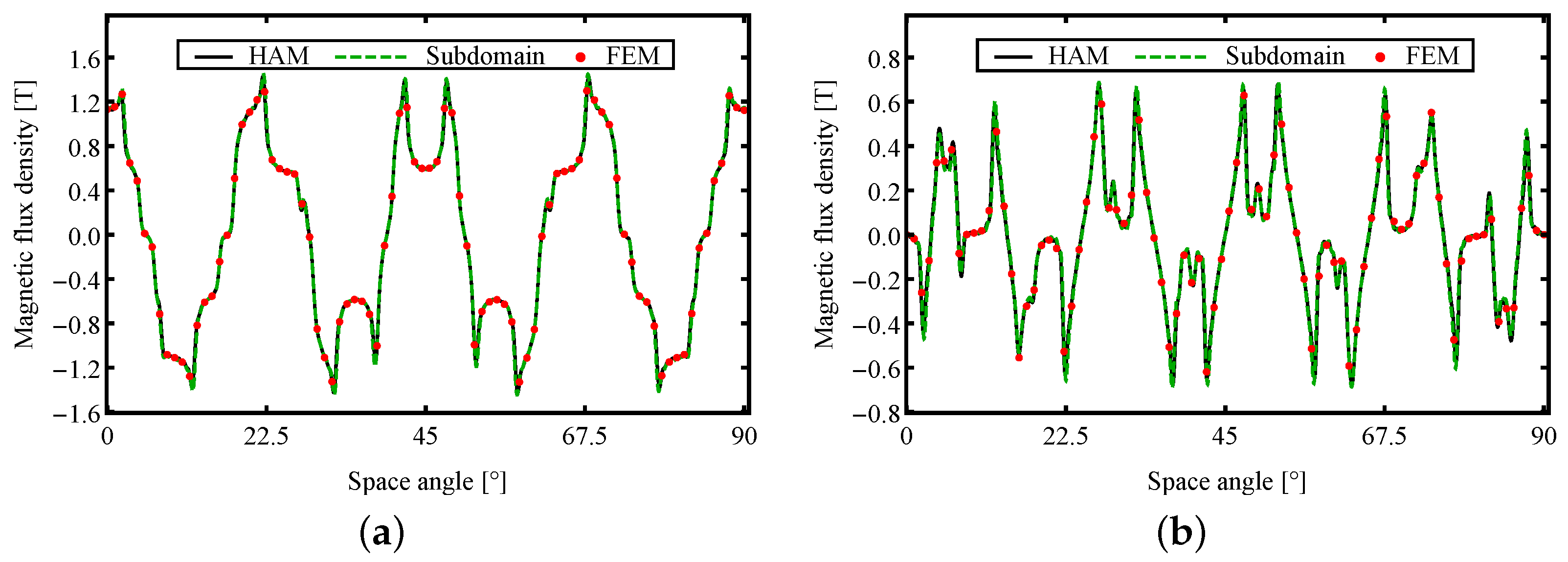
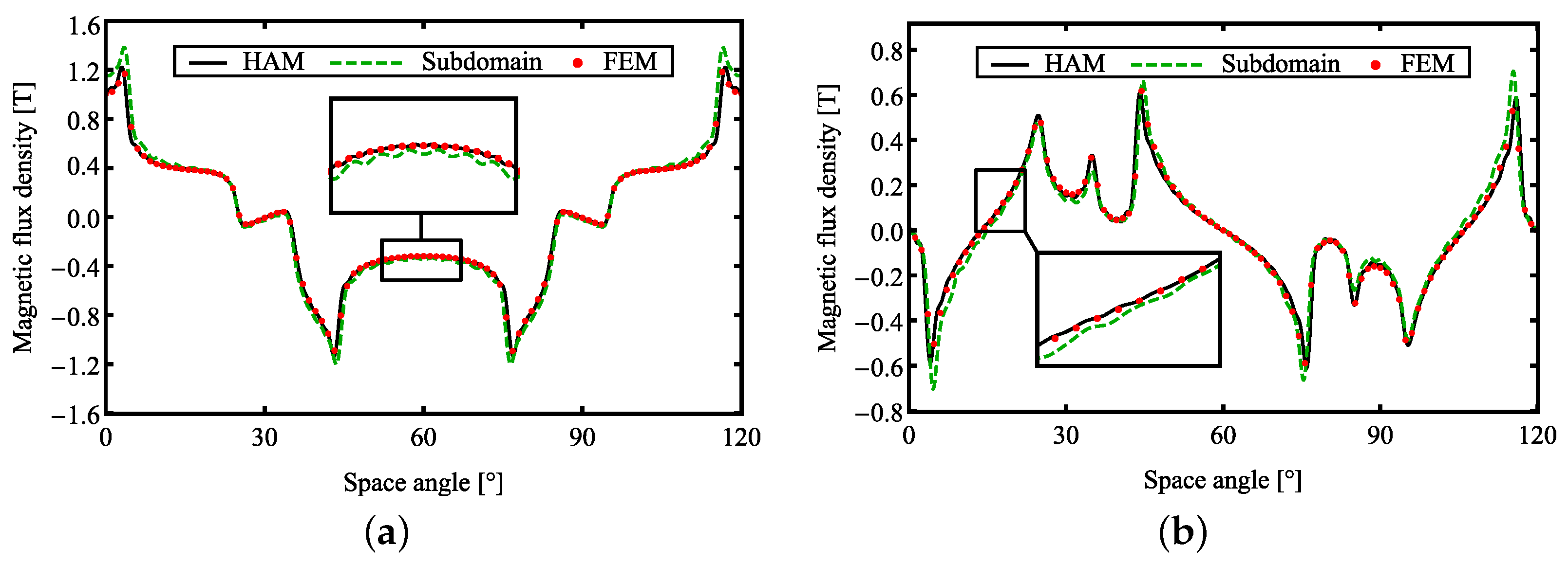
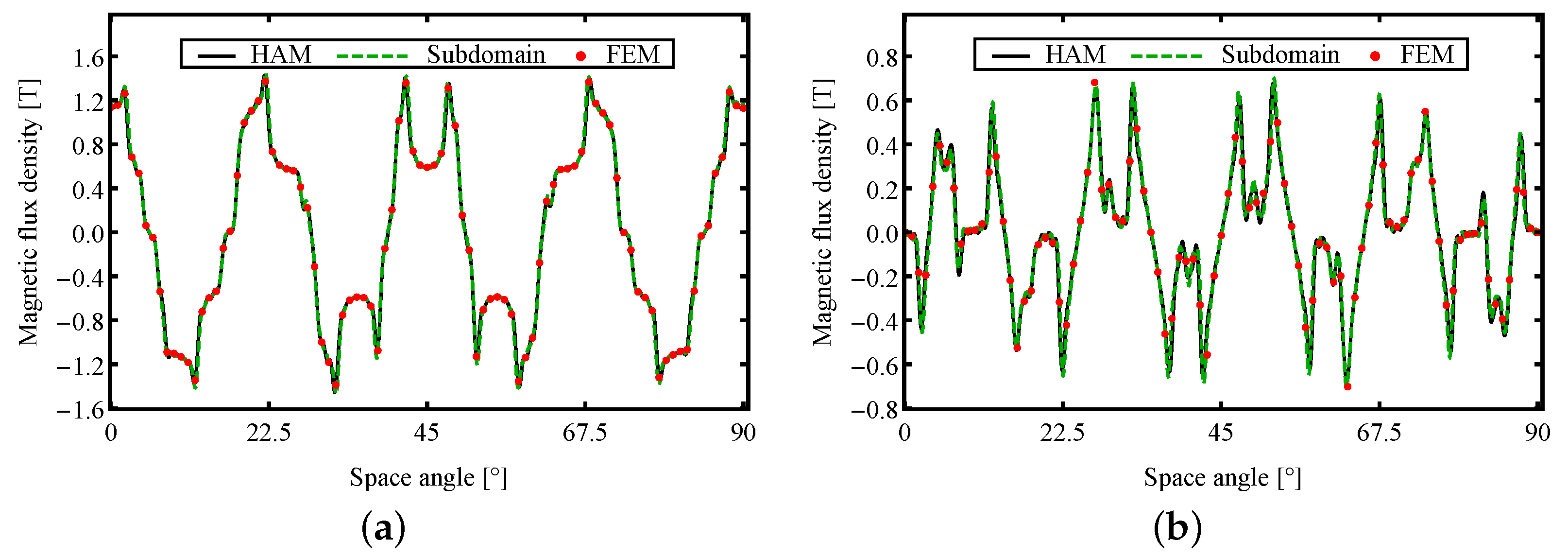
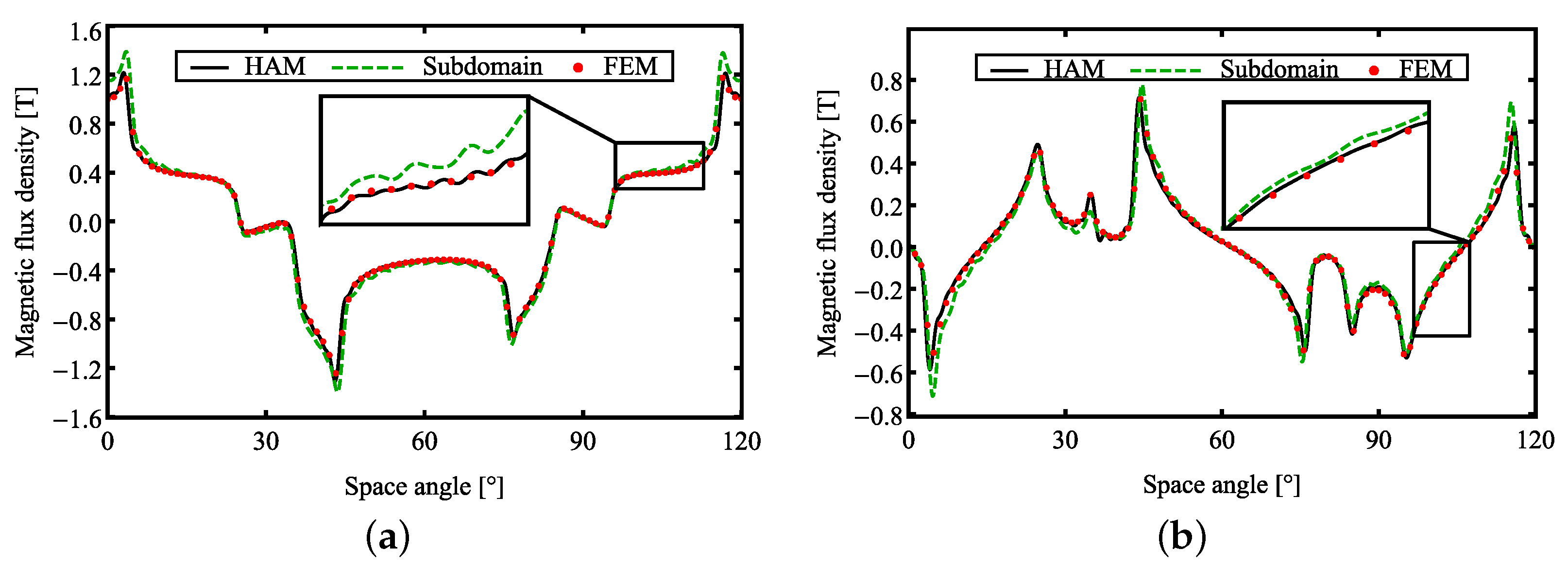
3.1. Fields
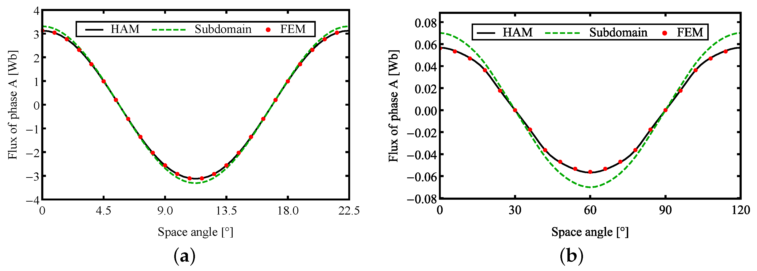
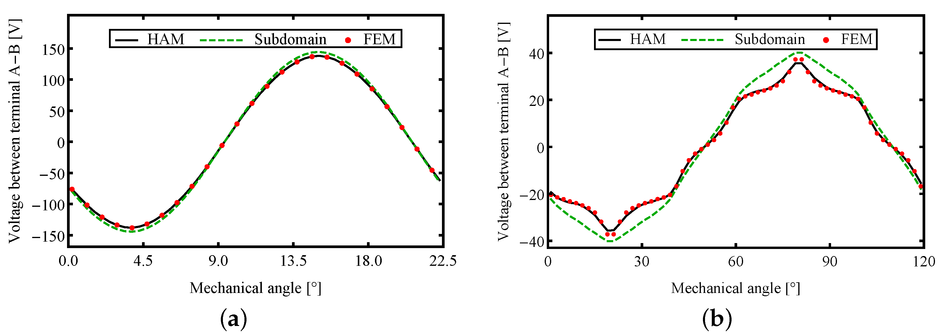
3.2. Flux and Back EMF
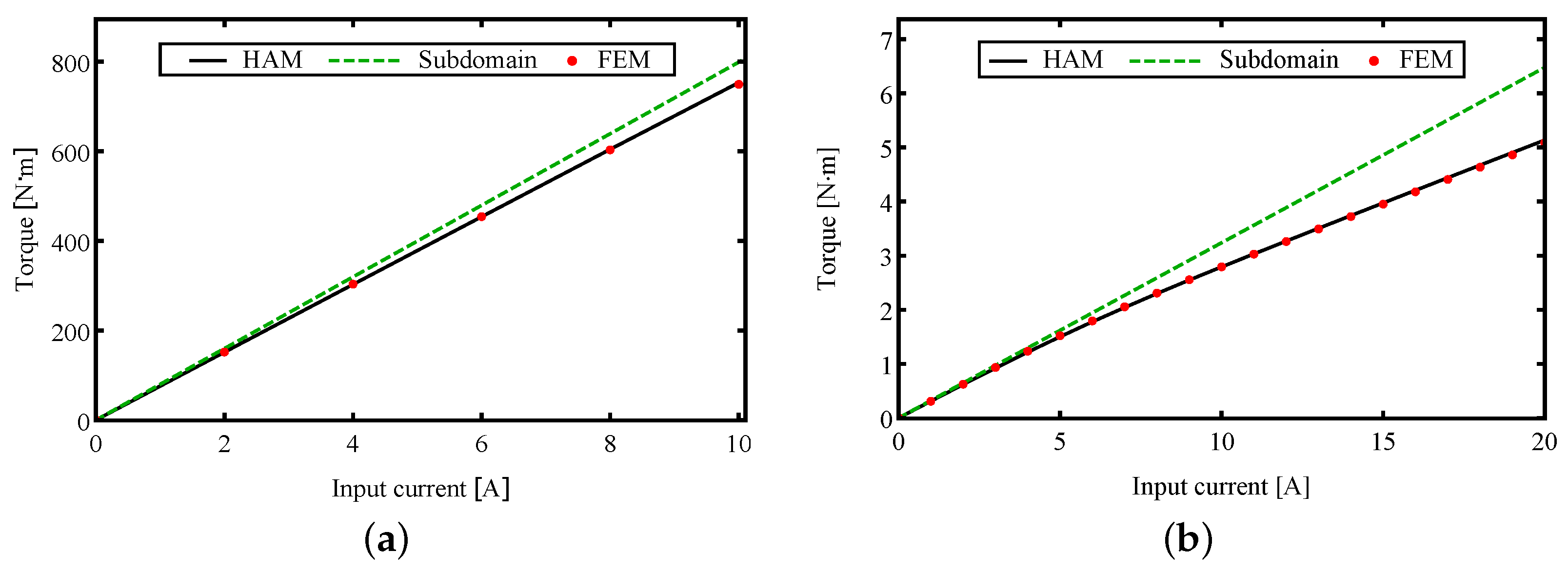
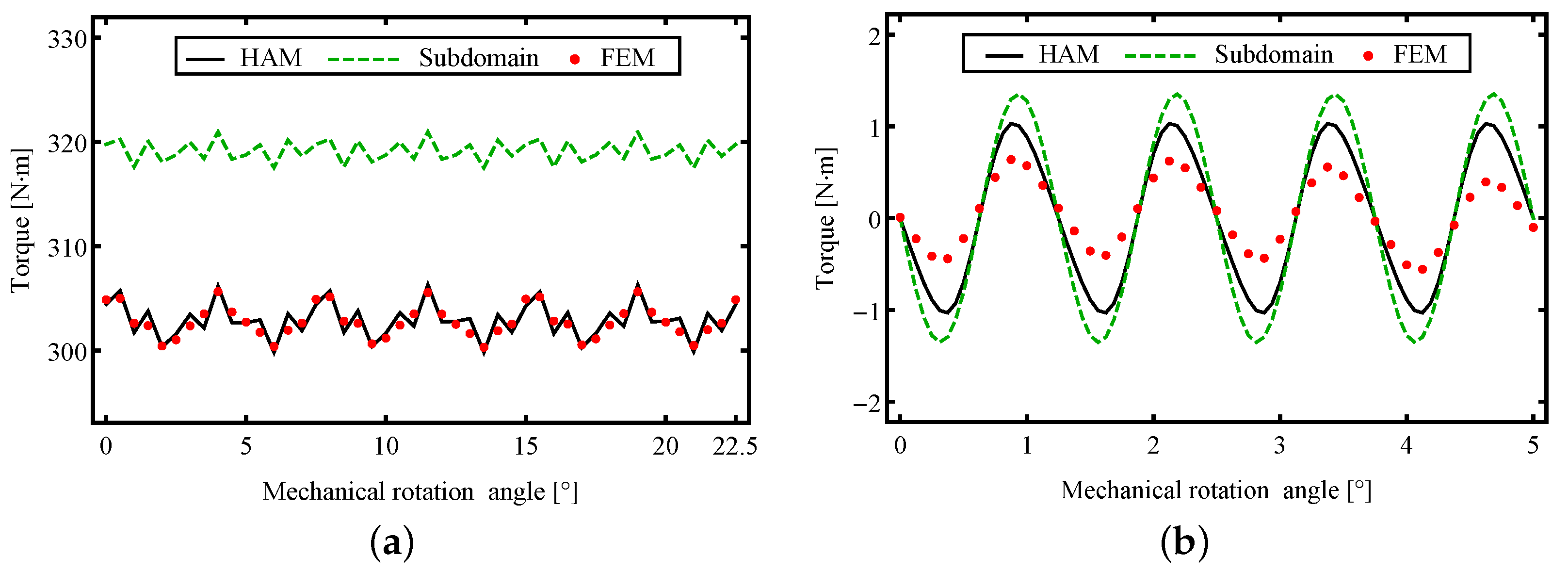
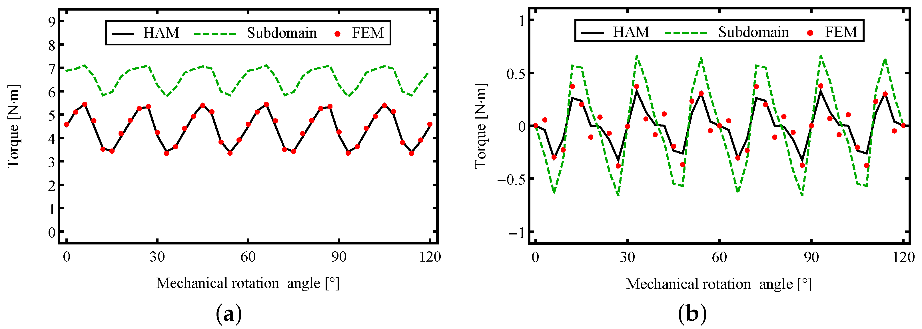
3.3. Torque
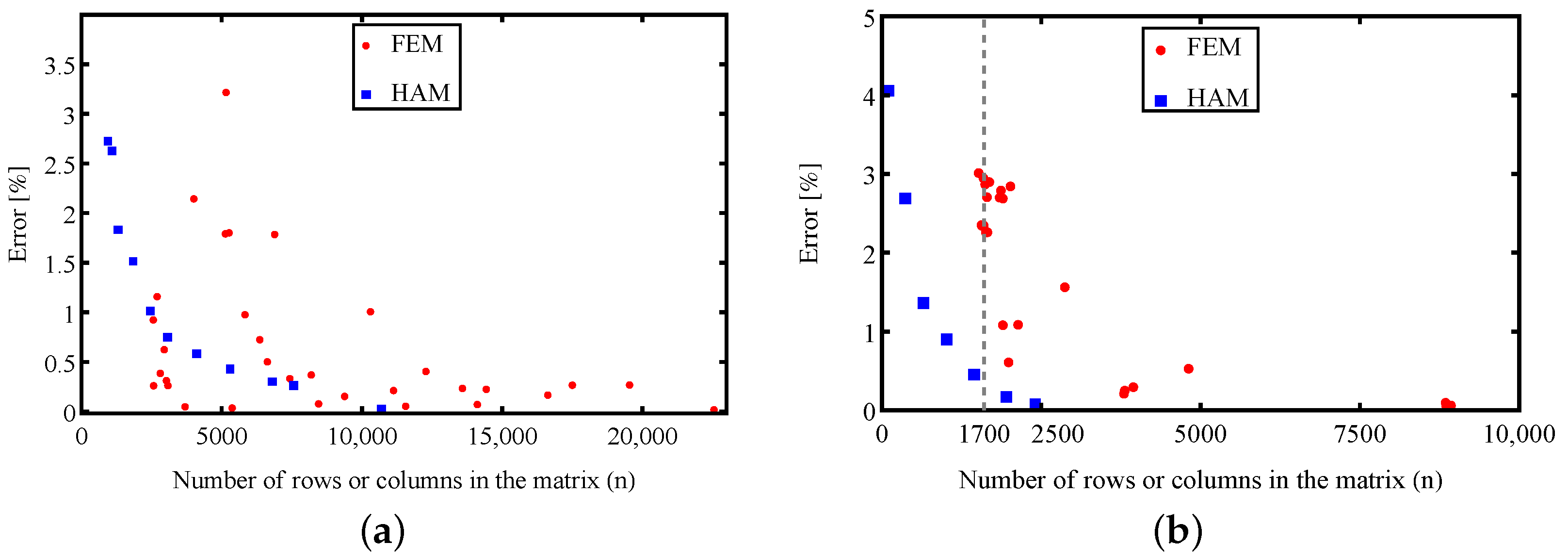
3.4. Multiple FEM and HAM Simulations
4. Conclusions
Author Contributions
Funding
Data Availability Statement
Conflicts of Interest
Abbreviations
| HAM | Hybrid analytical model |
| RN | Reluctance network |
| PM | Permanent magnet |
| EMF | Electromotive force |
| FEM | Finite-element method |
| CPM | Complex permeance method |
| MMF | Magnetomotive force |
Appendix A
Appendix B
References
- Gao, J.; Dai, L.; Zhang, W. Improved genetic optimization algorithm with subdomain model for multi-objective optimal design of SPMSM. CES Trans. Electr. Mach. Syst. 2018, 2, 160–165. [Google Scholar] [CrossRef]
- Ibala, A.; Rehbi, R.; Masmoudi, A. MEC-Based Modelling of Claw Pole Machines:Application to Automotive and Wind Generating Systems. Int. J. Renew. Energy Res. IJRER 2011, 1, 110–117. [Google Scholar]
- Rebhi, R.; Ibala, A.; Masmoudi, A. MEC-Based Sizing of a Hybrid-Excited Claw Pole Alternator. IEEE Trans. Ind. Appl. 2015, 51, 211–223. [Google Scholar] [CrossRef]
- Zhang, Z.; Sun, L.; Tao, Y.; Yan, Y. Development of nonlinear magnetic network model of a hybrid excitation doubly salient machine. In Proceedings of the 2013 International Electric Machines & Drives Conference, Chicago, IL, USA, 12–15 May 2013; pp. 663–669. [Google Scholar] [CrossRef]
- Pfister, P.D.; Yin, X.; Fang, Y. Slotted Permanent-Magnet Machines: General Analytical Model of Magnetic Fields, Torque, Eddy Currents, and Permanent-Magnet Power Losses Including the Diffusion Effect. IEEE Trans. Magn. 2016, 52, 1–13. [Google Scholar] [CrossRef]
- Hannon, B.; Sergeant, P.; Dupré, L.; Pfister, P.D. Two-Dimensional Fourier-Based Modeling of Electric Machines—An Overview. IEEE Trans. Magn. 2019, 55, 8107217. [Google Scholar] [CrossRef]
- Khedda, Z.D.; Boughrara, K.; Dubas, F.; Ibtiouen, R. Nonlinear Analytical Prediction of Magnetic Field and Electromagnetic Performances in Switched Reluctance Machines. IEEE Trans. Magn. 2017, 53, 8107311. [Google Scholar] [CrossRef]
- Dubas, F.; Boughrara, K. New Scientific Contribution on the 2-D Subdomain Technique in Cartesian Coordinates: Taking into Account of Iron Parts. Math. Comput. Appl. 2017, 22, 17. [Google Scholar] [CrossRef]
- Sprangers, R.L.J.; Paulides, J.J.H.; Gysen, B.L.J.; Lomonova, E.A. Magnetic Saturation in Semi-Analytical Harmonic Modeling for Electric Machine Analysis. IEEE Trans. Magn. 2016, 52, 8100410. [Google Scholar] [CrossRef]
- Liu, Z.; Bi, C.; Tan, H.; Low, T.S. A combined numerical and analytical approach for magnetic field analysis of permanent magnet machines. IEEE Trans. Magn. 1995, 31, 1372–1375. [Google Scholar] [CrossRef]
- Laoubi, Y.; Dhifli, M.; Verez, G.; Amara, Y.; Barakat, G. Open Circuit Performance Analysis of a Permanent Magnet Linear Machine Using a New Hybrid Analytical Model. IEEE Trans. Magn. 2015, 51, 8102304. [Google Scholar] [CrossRef]
- Laoubi, Y.; Dhifli, M.; Barakat, G.; Amara, Y. Hybrid analytical modeling of a flux switching permanent magnet machines. In Proceedings of the 2014 International Conference on Electrical Machines (ICEM), Berlin, Germany, 2–5 September 2014; pp. 1018–1023. [Google Scholar] [CrossRef]
- Wu, L.J.; Li, Z.; Huang, X.; Zhong, Y.; Fang, Y.; Zhu, Z.Q. A Hybrid Field Model for Open-Circuit Field Prediction in Surface-Mounted PM Machines Considering Saturation. IEEE Trans. Magn. 2018, 54, 8103812. [Google Scholar] [CrossRef]
- Wu, L.J.; Li, Z.K.; Wang, D.; Yin, H.; Huang, X.; Zhu, Z.Q. On-Load Field Prediction of Surface-Mounted PM Machines Considering Nonlinearity Based on Hybrid Field Model. IEEE Trans. Magn. 2019, 55, 8100911. [Google Scholar] [CrossRef]
- Li, Z.; Huang, X.; Wu, L.; Zhang, H.; Shi, T.; Yan, Y.; Shi, B.; Yang, G. An Improved Hybrid Field Model for Calculating On-Load Performance of Interior Permanent-Magnet Motors. IEEE Trans. Ind. Electron. 2021, 68, 9207–9217. [Google Scholar] [CrossRef]
- Tang, C.; Shen, M.; Fang, Y.; Pfister, P.D. Comparison of Subdomain, Complex Permeance, and Relative Permeance Models for a Wide Family of Permanent-Magnet Machines. IEEE Trans. Magn. 2021, 57, 8101205. [Google Scholar] [CrossRef]
- Wu, L.J.; Yin, H.; Wang, D.; Fang, Y. On-Load Field Prediction in SPM Machines by a Subdomain and Magnetic Circuit Hybrid Model. IEEE Trans. Ind. Electron. 2020, 67, 7190–7201. [Google Scholar] [CrossRef]
- Yin, H.; Wu, L.; Zheng, Y.; Fang, Y. Magnetic Field Prediction in Surface-Mounted PM Machines with Parallel Slot Based on a Nonlinear Subdomain and Magnetic Circuit Hybrid Model. In Proceedings of the 2019 IEEE International Electric Machines & Drives Conference (IEMDC), San Diego, CA, USA, 12–15 May 2019; pp. 1427–1432. [Google Scholar] [CrossRef]
- Zhu, Y.; Liu, G.; Xu, L.; Zhao, W.; Cao, D. A Hybrid Analytical Model for Permanent Magnet Vernier Machines Considering Saturation Effect. IEEE Trans. Ind. Electron. 2022, 69, 1211–1223. [Google Scholar] [CrossRef]
- Chikouche, B.L.; Boughrara, K.; Dubas, F.; Ibtiouen, R. Analytical magnetic field calculation for flat permanent-magnet linear machines with dual-rotor by using improved two-dimensional hybrid analytical method. COMPEL-Int. J. Comput. Math. Electr. Electron. Eng. 2021, 40, 602–623. [Google Scholar] [CrossRef]
- Ouagued, S.; Amara, Y.; Barakat, G. Cogging Force Analysis of Linear Permanent Magnet Machines Using a Hybrid Analytical Model. IEEE Trans. Magn. 2016, 52, 8202704. [Google Scholar] [CrossRef]
- Ouagued, S.; Amara, Y.; Barakat, G. Comparison of hybrid analytical modelling and reluctance network modelling for pre-design purposes. Math. Comput. Simul. 2016, 130, 3–21. [Google Scholar] [CrossRef]
- Zhu, Z.Q.; Wu, L.J.; Xia, Z.P. An Accurate Subdomain Model for Magnetic Field Computation in Slotted Surface-Mounted Permanent-Magnet Machines. IEEE Trans. Magn. 2010, 46, 1100–1115. [Google Scholar] [CrossRef]
- Zhu, Z.; Howe, D.; Bolte, E.; Ackermann, B. Instantaneous magnetic field distribution in brushless permanent-magnet DC motors. I. Open-circuit field. IEEE Trans. Magn. 1993, 29, 124–135. [Google Scholar] [CrossRef]


| Parameter | Machine I | Machine II | Unit |
|---|---|---|---|
| Pole pair number | 16 | 3 | - |
| Slot number | 36 | 9 | - |
| Number of turns | 113 | 50 | - |
| Lamination length | 140 | 54 | mm |
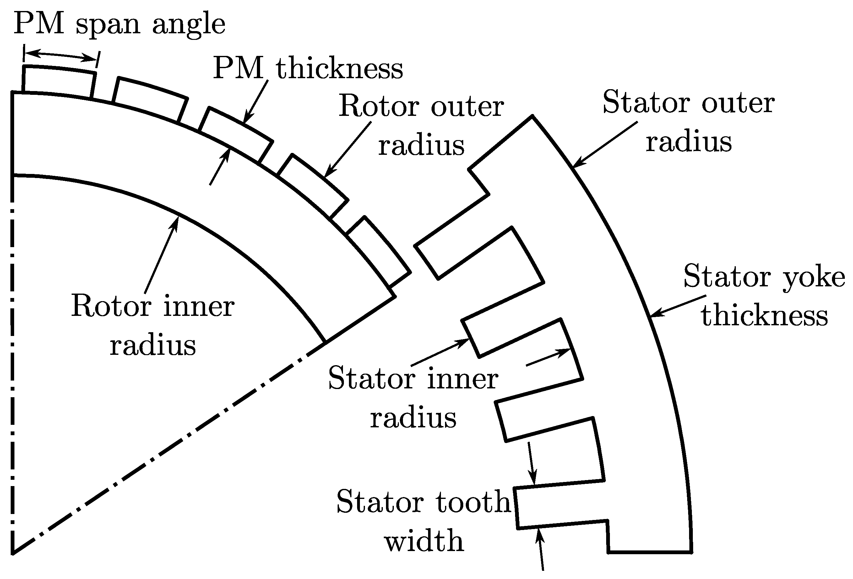
| Outer stator radius | 180 | 41 | mm |
| Inner stator radius | 134.2 | 22.3 | mm |
| Outer rotor radius | 133.1 | 21.8 | mm |
| Inner rotor radius | 114.5 | - | mm |
| Stator yoke thickness | 22 | 3 | mm |
| Stator tooth width | 10.7 | 3 | mm |
| PM thickness | 6.4 | 2.5 | mm |
| PM span angle | 9.2 | 50 | deg |
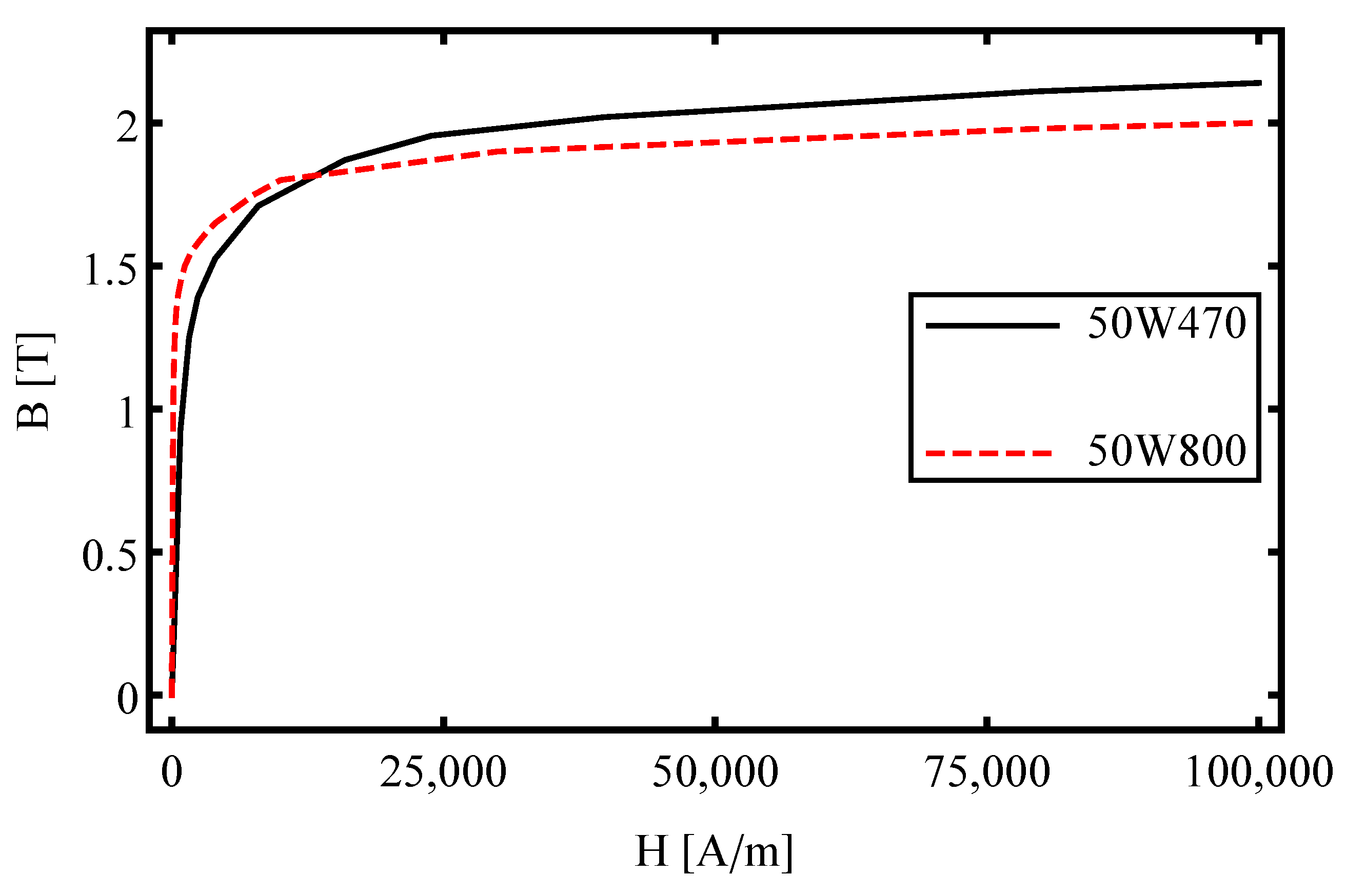
| Lamination material | 50W470 | 50W800 | - |
| PM remanent magnetic density | 1.32 | 1.20 | T |
| Permeability of PM | H/m |
Disclaimer/Publisher’s Note: The statements, opinions and data contained in all publications are solely those of the individual author(s) and contributor(s) and not of MDPI and/or the editor(s). MDPI and/or the editor(s) disclaim responsibility for any injury to people or property resulting from any ideas, methods, instructions or products referred to in the content. |
© 2023 by the authors. Licensee MDPI, Basel, Switzerland. This article is an open access article distributed under the terms and conditions of the Creative Commons Attribution (CC BY) license (https://creativecommons.org/licenses/by/4.0/).
Share and Cite
Lu, W.; Zhu, J.; Fang, Y.; Pfister, P.-D. A Hybrid Analytical Model for the Electromagnetic Analysis of Surface-Mounted Permanent-Magnet Machines Considering Stator Saturation. Energies 2023, 16, 1300. https://doi.org/10.3390/en16031300
Lu W, Zhu J, Fang Y, Pfister P-D. A Hybrid Analytical Model for the Electromagnetic Analysis of Surface-Mounted Permanent-Magnet Machines Considering Stator Saturation. Energies. 2023; 16(3):1300. https://doi.org/10.3390/en16031300
Chicago/Turabian StyleLu, Wenbiao, Jie Zhu, Youtong Fang, and Pierre-Daniel Pfister. 2023. "A Hybrid Analytical Model for the Electromagnetic Analysis of Surface-Mounted Permanent-Magnet Machines Considering Stator Saturation" Energies 16, no. 3: 1300. https://doi.org/10.3390/en16031300
APA StyleLu, W., Zhu, J., Fang, Y., & Pfister, P.-D. (2023). A Hybrid Analytical Model for the Electromagnetic Analysis of Surface-Mounted Permanent-Magnet Machines Considering Stator Saturation. Energies, 16(3), 1300. https://doi.org/10.3390/en16031300