Al-Biruni Earth Radius Optimization Based Algorithm for Improving Prediction of Hybrid Solar Desalination System

Abstract

The performance of a hybrid solar desalination system is predicted in this work using an enhanced prediction method based on a supervised machine-learning algorithm. A humidification–dehumidification (HDH) unit and a single-stage flashing evaporation (SSF) unit make up the hybrid solar desalination system. The Al-Biruni Earth Radius (BER) and Particle Swarm Optimization (PSO) algorithms serve as the foundation for the suggested algorithm. Using experimental data, the BER–PSO algorithm is trained and evaluated. The cold fluid and injected air volume flow rates were the algorithms’ inputs, and their outputs were the hot and cold fluids’ outlet temperatures as well as the pressure drop across the heat exchanger. Both the volume mass flow rate of hot fluid and the input temperatures of hot and cold fluids are regarded as constants. The results obtained show the great ability of the proposed BER–PSO method to identify the nonlinear link between operating circumstances and process responses. In addition, compared to the other analyzed models, it offers better statistical performance measures for the prediction of the outlet temperature of hot and cold fluids and pressure drop values.

1. Introduction

One of the necessities of existence, fresh water, is insufficiently accessible to billions of people worldwide. Although governments and humanitarian organizations have recently assisted many people living in water-stressed areas acquire access, the issue is expected to worsen due to the rapid population rise. About 97% of the water sources on earth are salty, and there are almost 800 million people who lack access to clean drinking water. Furthermore, by 2050, it is anticipated that 50% of the world’s water would be utilized [1]. Physical scarcity, which occurs when there is a lack of water due to regional ecological circumstances, and economic scarcity, which occurs when there is insufficient water infrastructure, are the two main types of water scarcity. Most experts agree that the Middle East and North Africa (MENA) region experiences the most physical water stress. The MENA region experiences lower rainfall than other places, yet several of its nations have rapidly expanding, highly populated urban areas that demand more water. However, many of these nations, particularly the wealthier ones, continue to fulfil their water needs. Desalination is a clever and practical solution that grows proportionally with population growth to the problem of freshwater resources. To address this issue successfully, numerous water desalination techniques have been employed. Due to their straightforward construction, long operational lives, and affordable clean water production, solar stills (SSs) are the most widely used technique of desalinating water. When combined with low-grade and renewable energy sources such as wind and solar, SS, which is seen as a promising entrant to the desalination process, gives an alternative way for lowering dependence on fossil fuels while also delivering different environmental benefits. SS, on the other hand, produces little. Therefore, numerous performance improvement initiatives were made to increase the output of SSs. Hybridization with other techniques, such as HDH, is one technique used to enhance the SS to achieve high performance. In order to produce a more cost-effective product, provide a better match between power demand and water requirements, and achieve the best possible combination of the properties of the two processes, a hybrid desalination system combines two or more processes [2]. Three models have been used to predict the effectiveness of solar stills and other desalination techniques. These models use numerical solutions [3], regression models [4], Artificial Neural Network (ANN) and machine learning technology, which is widely used in many energy system aspects based on actual experimental measurements, such as desalination systems [5].

ANNs are a prediction model and classification strategy when simulating complex interactions between sets of cause-and-effect variables or discovering patterns in data. Methods from transient detection, pattern recognition, approximation, and time series prediction are all potentially applicable [6,7]. ANN is a system of information processing that mimics how the human brain does. Neurons are the central component of this network, and they solve problems by collaborating. In situations where it is essential to extract the structure from existing data to formulate an algorithmic solution, a neural network comes in helpful [8,9]. Meta-heuristic algorithms are one of the most powerful techniques available for resolving challenges encountered in a variety of application contexts [10]. Most of these algorithms derive their logic from the physical algorithms present in the natural world. These optimization methods often yield acceptable solutions with minimal computational work and in a fair amount of time. Early detection of coronavirus can significantly reduce the spread of the disease, improving the prognosis for patients. This has led to the suggestion of several forms of artificial intelligence (AI) for use in solar desalination systems [11,12]. Ensemble method, the objective is to ensemble a prediction model by integrating the features of several independent base models. There are numerous ways in which this idea can be put into practice. Some more effective ways involve resampling the training set, while others use different prediction algorithms or tweak various parameters of the predictive strategy, etc. Finally, an ensemble of methods is used to combine the results of each prediction [13,14]. When more variables are included in the optimization process, Al-Biruni Earth Radius (BER) optimization algorithm [15] performs worse. Additionally, the algorithm’s convergence is premature. A significant advantage is the successful balancing of exploration and exploitation. The suggested method takes use of this advantage by using the BER algorithm. Despite its ease of use and balancing ability between exploration and exploitation, the Particle Swarm Optimization (PSO) algorithm [16] has drawbacks including performance declines when many local optimum solutions are present and a low exploration rate. This study employs the Al-Biruni Earth Radius optimizer to exploit the advantages and overcome the drawbacks of the PSO technique.

Based on measured values of water and air temperatures and yield, Kabeel and El-Said El-Said [17] offered some of the relations that help evaluate the hybrid desalination system (HDH-SSF) and the suggested BER–PSO classification model, excellent prediction accuracy of parameters include water yield, GOR, cost, and thermal efficiency is achieved. The proposed (BER–PSO) technique is initially applied to feature selection from the tested dataset using a binary version. The binary BER–PSO (bBER–PSO) algorithm is tested first compared to PSO [16], Grey Wolf Optimizer (GWO) [18], hybrid of PSO and GWO (GWO-PSO) [19], Whale Optimization Algorithm (WOA) [20], Biogeography-Based Optimizer (BBO) [21], Bowerbird Optimizer (SBO) [22], Firefly Algorithm (FA) [23], Genetic Algorithm (GA) [24], and Bat Algorithm (BA) [25]. The tested dataset is next assessed using a classifier built using the specified BER–PSO algorithm. Comparisons are made between the Decision Tree Regressor (DTR) [26], MLP Regressor (MLP) [27], K-Neighbors Regressor (KNR) [28], Support Vector Regression (SVR) [29], and Random Forest Regressor (RFR) [30] models and the “BER–PSO” algorithm. Additionally, two ensembles for creating new estimators are Average Ensemble (AVE) and Ensemble utilizing KNR (EKNR).

The following is a condensed list of the most important contributions that can be drawn from this body of work:

• Novel machine-learning techniques to predict the impact of various design and operational parameters on the thermos-fluid functionality of the HDH-SSF system.
• An improved Al-Biruni Earth Radius (BER) optimization-based Particle Swarm Optimization (BER–PSO) algorithm is suggested.
• The suggested algorithm’s binary variant, the binary BER–PSO algorithm, is used to select features from the dataset under test.
• For the purpose of raising the accuracy of tested dataset prediction, a BER–PSO-based classifier is introduced.
• The statistical significance of the BER–PSO algorithm can be determined by employing the Wilcoxon rank-sum and ANOVA tests.
• Both the binary BER–PSO and the BER–PSO-based classification algorithms can be tested for a variety of datasets.

The remaining portions of the document are arranged as follows. A description of the system and applications of AI is covered in Section 2. The methods utilized by machine learning (ML) to estimate the HDH-SSF’s thermos-fluid performance parameters are introduced in Section 3. Meanwhile, Section 4 presents a description of the proposed BER–PSO algorithm. Section 5 presents performance metrics, statistical parameters, experimental results, findings, and discussion. The study’s key conclusions are presented in Section 6.

2. Background

Based on Kabeel and El-Said [17], the experimental setup of the hybrid desalination system (HDH-SSF) is under investigation in this study. HDH-SSF system was primarily based on two concepts: the air humidification and dehumidification process (HDH), and the flash evaporation of saline water (SSF), as shown in Figure 1. A humidifier, dehumidifier (water cooled exchanger), air heater (flat plate collector), water heater (flat plate collector), and flashing evaporation unit make up the majority of the system. HDH system is made up of two loops, one for heating water and the other for heating air with a packed tower as a humidifier. Hot air passes through the humidifier and transfers the water that has evaporated to the dehumidifier, which cools to extract the fresh water. The condenser and flashing chamber are the main components of the single stage flashing evaporation system (SSF). Pump (P4) in the water loop delivers water from the mixing tank and splits it into two major lines, a feeding line and a bypass line, which are both controlled by valves (V15). The humidifier’s top is where the heated saline water is sprayed. The water drips to the humidifier’s bottom, where it is sent to a mixing tank for reheating. A centrifugal blower (placed on the humidifier’s input) pulls air from the atmosphere into the air loop, where it passes through the air solar heater. Hot air passes through the humidifier and transfers the water that has evaporated to the dehumidifier, which cools and dehumidifies the air. Condenser and flashing chamber make up the SSF system. In the closed loop of saline water flow between the flashing chamber and heat exchanger (HHEx), a portion of the salty water in the mixing tank (MT) is flowed to the helical heat exchanger (HHEx) to backup water, while the remainder is drained using valve (V5). Pumped to a flashing chamber under sub-atmospheric pressure, hot saline water from a heat exchanger evaporates by flashing. The condenser receives the water vapor that was extracted from the flashing chamber. The flashing unit condenser receives the saline-cooled water, which condenses the water vapor and discharges it. The bottom tray of the condenser holds the desalinated water, which is drawn up and pumped to the product tank. The pressure drop affects the flashing evaporation. In order to vacuum the condenser and flashing chamber, a vacuum pump is used. The rejected brine water from the humidifier is then combined with the saline water that exits the flashing unit condenser. Since the saline water is cold when it leaves the dehumidifier, it must be emptied. The following are some stages that can be used to illustrate the precise operational procedures of the experimental apparatus shown in Figure 1 [17]:

• Until the operational levels are reached, fill the system’s salty water loops.
• Set and modify the test case’s flow rates and temperature settings.
• Run the electrical heater (EH) and pump (P1) in the solar water heater loop until the tank’s water temperature (TK1) reaches the desired level.
• Set and modify the solenoid valve’s (SV1) open and closing periods in accordance with the flow rates of the backup water.
• Operate the vacuum pump (P3) until the desired pressure is reached inside the flashing chamber.
• Start the feeding pump (P2) to dispense saline water throughout the flashing chamber.
• Use the level indicator, water bleeding through valve (V4), and control valve (V8) to adjust the brine pool’s height.
• Turn on the air blower.
• Turn on the feeding pump (P4) to supply the salty water to the humidifier sprayers.
• Run the cooling water pump (P6) to pump the saline water to the condenser (C1) and dehumidifier.
• Run the circulation pump (P5) to pump the saline water mixing tank (C2)

The performance of the HDH-SSF system is predicted in this work using an enhanced prediction method based on a supervised machine-learning algorithm. It is essential to be aware of the intricate physical processes that occur inside the system. Some examples of these processes include the process of heat and mass transfer between water air streams, as well as the formation of humid air. Because of this, it is difficult to evaluate the effects of the design and operational parameters on the HDH-SSF’s thermal and economic performance [31,32,33]. Another difficult problem that needs to be taken into account is the existence of phase change processes. Additionally, the abrupt variations in the air and water streams’ temperature, and flow rate would cause a complicated behavior [34]. Therefore, it is believed that the variation in the air and water streams flow rates and temperature, are crucial parameters affect the performance of HDH-SSF. As a consequence, more emphasis should be given to analyzing its implications on the overall performance of hybrid desalination systems such as HDH-SSF, which includes thermos-fluid processes. The majority of the evaluation the effect of design and operational parameters on the HDH-SSF’s performance is conducted through the utilization of numerical and experimental methodologies. Mathematical problems involving complicated nonlinear systems should be solved with the use of simplified assumptions and numerical methods [35]. Contrarily, in experimental approaches, expensive and time-consuming trials are conducted out before system characteristics and the considered results are correlated statistically. Unfortunately, both approaches’ outcomes may be impacted by noisy circumstances [36]. Therefore, it would be ideal to create a reliable and accurate approach for simulating and forecasting the effects design and operational parameters on the HDH-SSF’s performance. Artificial intelligence-based algorithms can be learned by doing through a training process that is inspired by the brain [37]. Once trained, these algorithms can be a potent tool for predicting the link between the HDH-SSF parameters and the design and operational parameters. The ability of artificial intelligence approaches to generalize means that they can forecast behavior in situations that they were not exposed to during the training phase. By using these techniques, one can avoid issues with experimental methods, such as the use of low accuracy statistical-based correlations between HDH-SSF’s parameters derived from experimental data, or issues with numerical methods, such as those associated with solving nonlinear mathematical models [38]. The relationship between HDH-SSF design and operating variables is poorly understood and has not been the subject of extensive experimental research.

3. Materials and Methods

3.1. Al-Biruni Earth Radius (BER) Algorithm

The optimization procedure for the BER algorithm [15] begins by separating the population into two groups for exploration and exploitation. Agents are separated into subgroups, and within each subgroup, agents are dynamically adjusted to enhance the balancing ability between exploration and exploitation processes. The exploration group comprises 70 percent of the population, whereas the exploitation group comprises 30 percent. To raise the fitness levels of individuals in each group, the exploitation and exploration groups’ individuals are updated to allow for a more significant increase in the global average of individuals’ fitness. Mathematically, the agents in the exploration group seek out promising regions surrounding its current position in the search space. This is achieved by repeatedly looking for a higher option in terms of fitness value among the surrounding viable options. The following equations are used for this reason in the BER investigation:

Optimization algorithms discover the optimum solution given constraints. BER can depict a population member as a vector, $\mathbf{S}=S_1,S_2,\dots ,S_d\in R$, where $S_d$ is the search space size, and d is the optimization problem parameter or feature. Use the fitness function F to evaluate the agent’s performance up to a certain point. The optimization phases explore populations for a fitness-optimal vector ${\mathbf{S}}^{*}$.

3.1.1. Exploration Operation

Exploration finds intriguing portions of the search space and avoids local optimum stagnation by moving toward the optimal solution, as discussed below.

• The group’s lone explorer will utilize this strategy to find intriguing new areas to explore nearby. One must look through the many local possibilities to choose the best one. BER study uses the following equations:

  $$\mathbf{r}=h\frac{cos\left(x\right)}{1-cos\left(x\right)}$$

  (1)

  $$\mathbf{S}(t+1)=\mathbf{S}\left(t\right)+\mathbf{D}(2{\mathbf{r}}_2-1),\mathbf{D}={\mathbf{r}}_1(\mathbf{S}\left(t\right)-1)$$

  (2)

  where ${\mathbf{r}}_1$ and ${\mathbf{r}}_2$ are calculated by Equation (1), $0<x\le 180$, and h is within $[0,2]$. The vector $\mathbf{S}\left(t\right)$ represents a solution at iteration t, and $\mathbf{D}$ indicates circle diameter of search area.

3.1.2. Exploitation Operation

Exploitation teams must improve existing solutions. Each iteration, the BER honors the fittest participants. The BER uses two distinct methods to exploit.

• The equation that is presented here is utilized in order to proceed in the best solution direction.

  $$\mathbf{S}(t+1)={\mathbf{r}}^2(\mathbf{S}\left(t\right)+\mathbf{D}),\mathbf{D}={\mathbf{r}}_3(\mathbf{L}\left(t\right)-\mathbf{S}\left(t\right))$$

  (3)

  where vector $\mathbf{L}\left(t\right)$ denotes the best solution, vector $\mathbf{S}\left(t\right)$ represents the solution at iteration t, and $\mathbf{D}$ is the distance vector. ${\mathbf{r}}_3$ is a random vector that is calculated using Equation (1), and it governs the movement steps that are taken towards the best solution.
• The area surrounding the best solution constitutes an interesting potential choice. Individuals will find ways to improve the situation by investigating possibilities somewhat close to the best solution. To complete the aforementioned process, the BER will apply the following equation.

  $${\mathbf{S}}^{\prime }(t+1)=\mathbf{r}({\mathbf{S}}^{*}\left(t\right)+\mathbf{k}), \mathbf{k}=1+\frac{2\times t^2}{T_{max}^2}$$

  (4)

  where ${\mathbf{S}}^{*}\left(t\right)$ denotes the best solution to the problem. Following a comparison of the $\mathbf{S}(t+1)$ and ${\mathbf{S}}^{\prime }(t+1)$ it is possible to pick the ${\mathbf{S}}^{*}$ option as the optimal one. If the best fitness has not changed during the course of the preceding two iterations, the solution will be updated in accordance with the following equation.

  $$\mathbf{S}(t+1)=\mathbf{k}\ast z^2-h\frac{cos\left(x\right)}{1-cos\left(x\right)}$$

  (5)

  where z denotes random value within $[0,1]$.

3.1.3. Selection of the Best Solution

The BER chooses the best for the next cycle to ensure high-quality solutions. Mutation and exploration group members give the BER excellent exploration capabilities. BER exploration delays convergence. Algorithm 1 shows BER pseudo-code. The BER receives size of population, rate of mutation, and maximum iterations. The BER splits participants into exploratory and exploitative groups. The BER algorithm dynamically alters group sizes during iterative solution search. Each team performs tasks in two ways. To ensure variety and depth, the BER shuffles answers between iterations. An exploration group solution may progress to the exploitation group in the next iteration. BER elitism prevents leader replacement.

Algorithm 1 AL-Biruni earth radius (BER) algorithm

1: Initialize BER population ${\mathbf{S}}_i(i=1,2,\dots ,d)$ with population size of d, maximum iterations of $T_{max}$, objective function $F_n$, $t=1$, and other parameters 2: Calculate objective function $F_n$ for each agent ${\mathbf{S}}_i$ 3: Find the best solution and denote it as ${\mathbf{S}}^{*}$ 4: Divide agents into exploration group, $n_1$, and exploitation group, $n_2$ 5: while$t\le T_{max}$do 6:    Update $\mathbf{r}=h\frac{cos\left(x\right)}{1-cos\left(x\right)}$, ${\mathbf{r}}_1=h_1\frac{cos\left(x\right)}{1-cos\left(x\right)}$, ${\mathbf{r}}_2=h_2\frac{cos\left(x\right)}{1-cos\left(x\right)}$, ${\mathbf{r}}_3=h_3\frac{cos\left(x\right)}{1-cos\left(x\right)}$ 7:    for ($i=1:i<n_1+1$) do 8:      Find parameter $\mathbf{D}$ as ${\mathbf{r}}_1(\mathbf{S}\left(t\right)-1)$ 9:      Update agents’ positions as $\mathbf{S}(t+1)=\mathbf{S}\left(t\right)+\mathbf{D}(2{\mathbf{r}}_2-1)$ 10:    end for 11:    for ($i=1:i<n_2+1$) do 12:      Find parameter $\mathbf{D}$ as ${\mathbf{r}}_3(\mathbf{L}\left(t\right)-\mathbf{S}\left(t\right))$ 13:      Update agents’ positions as $\mathbf{S}(t+1)={\mathbf{r}}^2(\mathbf{S}\left(t\right)+\mathbf{D})$ 14:      Calculate parameter $\mathbf{k}$ as $1+\frac{2\times t^2}{Ma{x}_{iter}^2}$ 15:      Update agents’ positions around the best solution as ${\mathbf{S}}^{\prime }(t+1)=\mathbf{r}({\mathbf{S}}^{*}\left(t\right)+\mathbf{k})$ 16:      Compare $\mathbf{S}(t+1)$ and ${\mathbf{S}}^{\prime }(t+1)$ and select the best solution as ${\mathbf{S}}^{*}$ 17:      if best value of objective function is the same for last two rounds then 18:        Mutate the solution using $\mathbf{S}(t+1)=\mathbf{k}\ast z^2-h\frac{cos\left(x\right)}{1-cos\left(x\right)}$ 19:      end if 20:    end for 21:    Update objective function $F_n$ for each agent ${\mathbf{S}}_i$ 22:    Update the parameters, $t=t+1$ 23: end while 24: Return${\mathbf{S}}^{*}$

3.2. Particle Swarm Optimization (PSO) Algorithm

In the PSO algorithm, potential solutions (particles) in the search space, imitating the natural bird swarms intelligence [16]. A particle’s velocity is the pace at which it changes location. Throughout time, the positions of the particles are modified. Throughout its flight, a particle’s speed is stochastically increased to its previous best location. The position vector is denoted by ${\mathbf{S}}_i(i=1,2,\dots ,n)$ with size n while the velocity vector is denoted by ${\mathbf{V}}_i(i=1,2,\dots ,n)$. The following equations are applied to update the particle at iteration $t+1$ to a region close to the optimal solution.

$$\mathbf{S}(t+1)=\mathbf{S}\left(t\right)+\mathbf{V}(t+1),$$

(6)

$$\mathbf{V}(t+1)=\mathbf{V}\left(t\right)+C_1{g}_1(\left({\mathbf{S}}^{*}\right)+\mathbf{S}\left(t\right))+C_2{g}_2({\mathbf{S}}_{gbest}-\mathbf{S}\left(t\right))$$

(7)

where $g_1$ and $g_2$ are random variables within [0, 1], and $C_1$ and $C_2$ are constants.

4. Proposed BER–PSO Algorithm

The proposed BER–PSO algorithm uses the advantages of both BET and PSO algorithms. Algorithm 2 shows the steps of the proposed algorithm. The algorithm starts by initializing the population positions ${\mathbf{S}}_i(i=1,2,\dots ,n)$ and velocities ${\mathbf{V}}_i(i=1,2,\dots ,n)$ with n agents—the parameters of the BER and PSO algorithms and the maximum iterations and objective function $f_n$. The objective function is then calculated for each ${\mathbf{S}}_i$, and the best agent $\left({\mathbf{S}}^{*}\right)$ is selected. During the iterations, the proposed algorithm swaps between the BER and PSO algorithms to update the agents. Finally, the optimal solution $\left({\mathbf{S}}^{*}\right)$ is calculated.

Algorithm 2 Proposed BER–PSO algorithm

1: Initialize BER–PSO population positions ${\mathbf{S}}_i(i=1,2,\dots ,d)$ with population size d, maximum iterations $T_{max}$, objective function $F_n$, $t=1$, and other parameters 2: Calculate objective function $F_n$ for each agent ${\mathbf{S}}_i$ 3: Find the best solution as ${\mathbf{S}}^{*}$ 4: Divide agents into exploration group, $n_1$, and exploitation group, $n_2$ 5: while$t\le T_{max}$do 6:    if ($t\%2$) then 7:      Update $\mathbf{r}=h\frac{cos\left(x\right)}{1-cos\left(x\right)}$, ${\mathbf{r}}_1=h_1\frac{cos\left(x\right)}{1-cos\left(x\right)}$, ${\mathbf{r}}_2=h_2\frac{cos\left(x\right)}{1-cos\left(x\right)}$, ${\mathbf{r}}_3=h_3\frac{cos\left(x\right)}{1-cos\left(x\right)}$ 8:      for ($i=1:i<n_1+1$) do 9:           Calculate parameter $\mathbf{D}$ as ${\mathbf{r}}_1(\mathbf{S}\left(t\right)-1)$ 10:         Update agents’ positions as $\mathbf{S}(t+1)=\mathbf{S}\left(t\right)+\mathbf{D}(2{\mathbf{r}}_2-1)$ 11:      end for 12:      for ($i=1:i<n_2+1$) do 13:         Calculate parameter $\mathbf{D}$ as ${\mathbf{r}}_3(\mathbf{L}\left(t\right)-\mathbf{S}\left(t\right))$ 14:         Update agents’ positions as $\mathbf{S}(t+1)={\mathbf{r}}^2(\mathbf{S}\left(t\right)+\mathbf{D})$ 15:         Calculate $\mathbf{k}=1+\frac{2\times t^2}{Ma{x}_{iter}^2}$ 16:         Update agents’ positions around the best solution as ${\mathbf{S}}^{\prime }(t+1)=\mathbf{r}({\mathbf{S}}^{*}\left(t\right)+\mathbf{k})$ 17:         Compare $\mathbf{S}(t+1)$ and ${\mathbf{S}}^{\prime }(t+1)$ and select the best solution ${\mathbf{S}}^{*}$ 18:         if best value of objective function is the same for last two rounds then 19:            Mutate solution as $\mathbf{S}(t+1)=\mathbf{k}\ast z^2-h\frac{cos\left(x\right)}{1-cos\left(x\right)}$ 20:         end if 21:      end for 22:    else 23:      Update velocities as $\mathbf{V}(t+1)=\mathbf{V}\left(t\right)+C_1{g}_1(\left({\mathbf{S}}^{*}\right)+\mathbf{S}\left(t\right))+C_2{g}_2({\mathbf{S}}_{gbest}-\mathbf{S}\left(t\right))$ 24:      Update agents’ positions as $\mathbf{S}(t+1)=\mathbf{S}\left(t\right)+\mathbf{V}(t+1)$ 25:    end if 26:    Update objective function $F_n$ for each agent ${\mathbf{S}}_i$ 27:    Update the BER–PSO parameters, $t=t+1$ 28: end while 29: Return${\mathbf{S}}^{*}$

4.1. Computational Complexity

The computational complexity of the BER–PSO algorithm is denoted as follows. The complexity is defined as follows for iterations $T_{max}$ with a population of n.

• Initialize BER–PSO parameters: O(1).
• Calculate fitness function for each agent: O(n).
• Get the best agent: O (n).
• Update agents’ positions: O($T_{max}\times n$).
• Update agents’ positions around best solution: O($T_{max}\times n$).
• Compare positions to select best solution: O($T_{max}\times n$).
• Mutate solutions: O($T_{max}\times n$).
• Update velocities: O($T_{max}\times n$).
• Update positions to head toward best solution: O($T_{max}\times n$).
• Update fitness function: O($T_{max}$).
• Update BER–PSO parameters: O($T_{max}$).
• Get best agent ${\mathbf{x}}_{Gbest}$: O(1)

The computation complexity is chosen at based on the BER–PSO algorithm analysis that was conducted above to O($T_{max}\times n$) and to O($T_{max}\times n\times d$) for d dimension.

4.2. Proposed Binary BER–PSO Algorithm

To make the process of choosing features from the dataset easier, the continuous values of the proposed BER–PSO algorithm will be converted to binary [0,1] in this section. In the event of feature selection concerns, the BER–PSO algorithm answers can be strictly binary [0 or 1] by utilizing the following equation.

The following equation is used in this investigation and is based on the $Sigmoid$ function [39].

$$\begin{array}{cc}\hfill & x_d^{t+1}=\left\{\begin{array}{cc}1\hfill & \mathrm{if}Sigmoid\left(m\right)\ge 0.5\hfill \\ 0\hfill & otherwise\hfill \end{array}\right.,\hfill \\ & Sigmoid\left(m\right)={\displaystyle \frac{1}{1+e^{-10(m-0.5)}}},\hfill \end{array}$$

(8)

where the binary answer at iteration t and dimension d is indicated by $x_d^{t+1}$. The output solutions can be scaled to be binary ones using the $Sigmoid$ function. The value will change to 1 if $Sigmoid\left(m\right)\ge 0.5$, otherwise it will remain at 0. The algorithm’s chosen features are reflected in the m parameter. In Algorithm 3, the binary BER–PSO algorithm is thoroughly explained. The computing complexity of the BER–PSO method is determined to be O($t_{max}\times n$) and will be O($t_{max}\times n\times d$) for the d dimension.

Algorithm 3 Proposed Binary BER–PSO algorithm.

1: Initialize the BER–PSO parameters and population 2: Convert solution to binary [0 or 1] 3: Calculate objective function for each agent 4: Find best solution 5: Divide agents into exploration group, $n_1$, and exploitation group, $n_2$ 6: while$t\le T_{max}$do 7:    if ($t\%2$) then 8:        for ($i=1:i<n_1+1$) do 9:           Update agents’ positions 10:      end for 11:      for ($i=1:i<n_2+1$) do 12:           Update agents’ positions 13:           Update agents’ positions around best solution 14:           Compare updated positions and select the best solution 15:           if best value of objective function is the same for last two rounds then 16:             Mutate solution 17:           end if 18:      end for 19:    else 20:      Update agents’ velocities and positions 21:    end if 22:    Convert updated solution to binary 23:    Update objective function for each individual 24:    Update the BER–PSO parameters 25: end while 26: Return best solution

5. Experimental Results

The findings of this investigation are thoroughly explained in this section. There are two different situations for the experiments. The first case covers the BER–PSO algorithm’s feature selection capabilities for the dataset under test, while the second scenario demonstrates the algorithm’s classification capabilities. In the tested dataset, the volume flow rates, temperatures, and weather conditions were the inputs to the algorithms, and the outputs of the algorithms were the outlet temperatures of the air and water as well as the humidity added by the humidifier.

5.1. Feature Selection Scenario

The proposed (BER–PSO) algorithm’s binary version is employed to choose features from the dataset under test. The feature selection outcomes of the BER–PSO method provided in this work are examined in the first scenario.

Table 1. Parameters for BER–PSO algorithm configuration.

Parameter (s)	Value (s)
No. of Agents	10
No. of Iterations	80
No. of Runs	20
Dimension	No. of features
$W_{max}$, $W_{min}$	[0.9, 0.6]
$C_1$, $C_2$	[2, 2]
$\alpha$ of $F_n$	0.99
$\beta$ of $F_n$	0.01

displays the configuration of the BER–PSO method for each parameter utilized in the experiment, while

Table 2. Parameter settings for the compared algorithms.

Algorithm	Parameter (s)	Value (s)
PSO	Acceleration constants	[2, 2]
	Inertia $W_{max}$, $W_{min}$	[0.6, 0.9]
	Particles	10
	Iterations	80
GWO	a	2 to 0
	Iterations	80
	Wolves	10
GA	Cross over	0.9
	Mutation ratio	0.1
	Selection mechanism	Roulette wheel
	Iterations	80
	Agents	10
WOA	r	[0, 1]
	Iterations	80
	Whales	10
	a	2 to 0
SBO	Size of step	0.94
	Mutation probability	0.05
	Upper and lower limit	0.02
FA	Number of fireflies	10
BA	Pluse rate	0.5
	Loudness	0.5
	Frequency	[0, 1]
BBO	Probability of Immigration	[0, 1]
	Probability of Mutation	0.05
	Probability of Habitat modification	1.0
	Size of step	1.0
	Rate of migration	1.0
	Maximum immigration	1.0

displays the configuration of the comparison algorithms. PSO [16], GWO [18], hybrid GWO-PSO [19], WOA [20], BBO [21], SBO [22], FA [23], GA [24], and BA [25] are tested against the binary BER–PSO (bBER–PSO) algorithm.

In the binary BER–PSO method, the quality of a solution is assessed using the objective equation, ${\mathbf{f}}_n$. The following objective equation, ${\mathbf{f}}_n$, includes total number of features, S, number of selected features, s, and classifier’s error rate, $Err$.

$${\mathbf{f}}_n=\alpha Err+\beta {\displaystyle \frac{\left|s\right|}{\left|S\right|}}$$

(9)

where $\beta =1-\alpha$ and $\alpha \in [0,1]$ denote the population significance of the provided trait. If the method can offer a subset of features with a low classification error rate, it is successful. K-nearest neighbor (k-NN) is a popular and simple categorization method. This method makes use of the k-NN as a classifier to guarantee the validity of the features selected. The shortest distance between the query instance and the training instances is the sole criterion for classifier selection; this experiment does not make use of a K-nearest neighbor model.

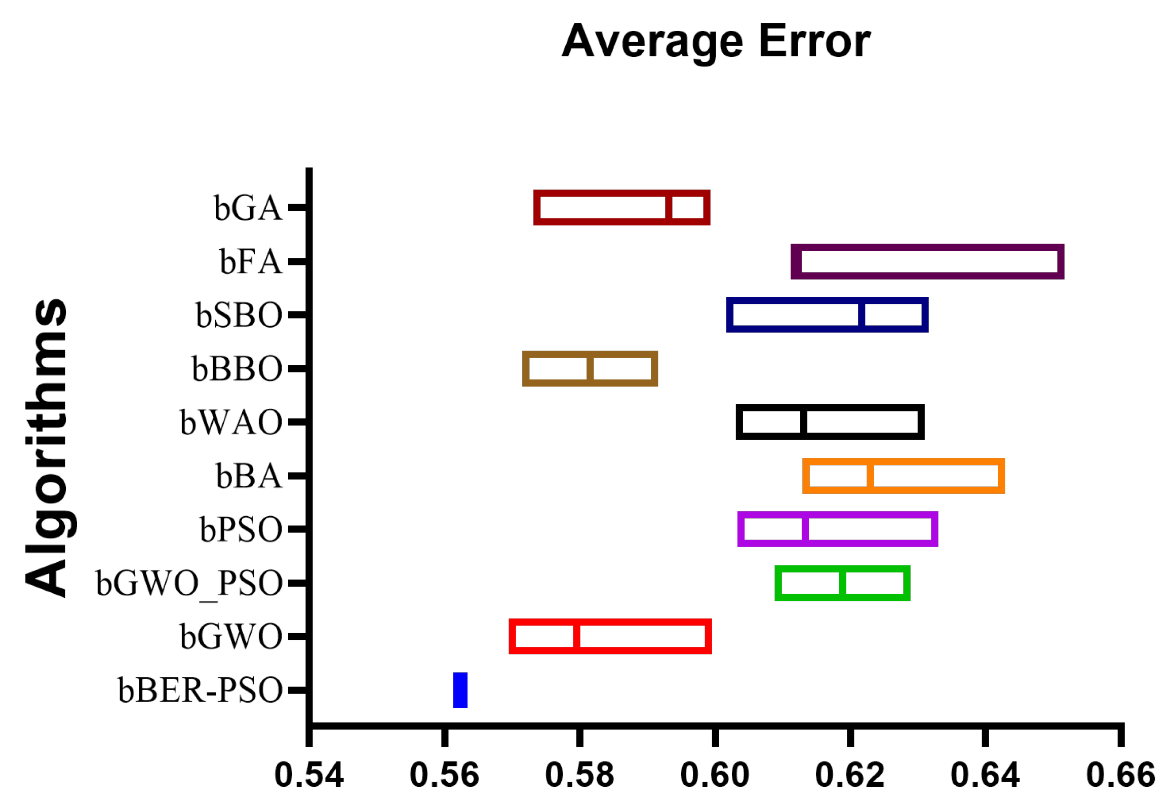
The performance metrics used in this experiment are average error, average select size, average fitness, best fitness, worst fitness, and standard deviation, as listed mathematically in

Table 3. Feature selection performance metrics.

Metric	Value
Average Error	$1-\frac{1}{M}{\sum }_{j=1}^M\frac{1}{N}{\sum }_{i=1}^{N}Match(C_i,L_i)$
Average Select Size	$\frac{1}{M}{\sum }_{j=1}^M{\displaystyle \frac{size\left(g_j^{*}\right)}{D}}$
Average Fitness	$\frac{1}{M}{\sum }_{j=1}^M{g}_j^{*}$
Best Fitness	$Mi{n}_{j=1}^M{g}_j^{*}$
Worst Fitness	$Ma{x}_{j=1}^M{g}_j^{*}$
Standard Deviation	$\sqrt{\frac{1}{M-1}\sum {(g_j^{*}-Mean)}^2}$

.

Table 4. Results of the proposed bBER–PSO algorithm and comparison.

Performance Metric	bBER–PSO	bGWO	bGWO_PSO	bPSO	bBA	bWOA	bBBO	bSBO	bFA	bGA
Average error	0.5623	0.5795	0.6188	0.6133	0.6229	0.6131	0.5815	0.6216	0.6117	0.5931
Average Select size	0.5151	0.7151	0.8484	0.7151	0.8545	0.8785	0.8789	0.8854	0.7496	0.6575
Average Fitness	0.6255	0.6417	0.65	0.6401	0.663	0.6479	0.6458	0.6798	0.692	0.6531
Best Fitness	0.5273	0.562	0.6035	0.6204	0.5527	0.612	0.6355	0.6229	0.6107	0.5564
Worst Fitness	0.6258	0.6289	0.7135	0.6881	0.6543	0.6881	0.722	0.7026	0.7083	0.6715
Standard deviation Fitness	0.4478	0.4525	0.4707	0.4519	0.4618	0.4541	0.4968	0.5128	0.4887	0.4541

shows the out results for the presented bBER–PSO algorithm and compared algorithms. The bBER–PSO algorithm gives an average error of 0.5623, which is better than other algorithms. The second-best average error of (0.5795) is achieved by bGWO, while the worst average error of (0.6229) is achieved by bBA. The box plot analysis of the presented bBER–PSO and compared algorithms is also presented in Figure 2. The bBER–PSO algorithm shows better results over 15 runs over average error metric.

Statistical analysis is performed to confirm the algorithm’s performance.

Table 5. Results of an ANOVA test comparing the presented bBER–PSO method to other algorithms.

	SS	DF	MS	F (DFn, DFd)	p Value
Treatment (between columns)	0.06272	9	0.006969	F (9, 140) = 184.1	p < 0.0001
Residual (within columns)	0.005299	140	3.79 × 10${}^{-5}$	-	-
Total	0.06802	149	-	-	-

shows the ANOVA test results of the presented bBER–PSO algorithm versus compared algorithms.

Table 6. Results of the provided bBER–PSO method and compared algorithms in the Wilcoxon Signed Rank Test.

	bBER–PSO	bGWO	bGWO_PSO	bPSO	bBA	bWAO	bBBO	bSBO	bFA	bGA
Theoretical median	0	0	0	0	0	0	0	0	0	0
Actual median	0.5623	0.5795	0.6188	0.6133	0.6229	0.6131	0.5815	0.6216	0.6117	0.5931
Number of values	15	15	15	15	15	15	15	15	15	15
Wilcoxon Signed Rank Test
Sum of signed ranks (W)	120	120	120	120	120	120	120	120	120	120
Sum of positive ranks	120	120	120	120	120	120	120	120	120	120
Sum of negative ranks	0	0	0	0	0	0	0	0	0	0
p value (two tailed)	<0.0001	<0.0001	<0.0001	<0.0001	<0.0001	<0.0001	<0.0001	<0.0001	<0.0001	<0.0001
Exact or estimate?	Exact	Exact	Exact	Exact	Exact	Exact	Exact	Exact	Exact	Exact
Significant (alpha = 0.05)?	Yes	Yes	Yes	Yes	Yes	Yes	Yes	Yes	Yes	Yes
How big is the discrepancy?
Discrepancy	0.5623	0.5795	0.6188	0.6133	0.6229	0.6131	0.5815	0.6216	0.6117	0.5931

presents the Wilcoxon Signed Rank test results of the presented bBER–PSO algorithm and compared algorithms over 15 runs. The ANOVA and Wilcoxon Signed Rank tests results confirm the performance of the bBER–PSO algorithm.

5.2. Classification Scenario

The HDH and SSF test data classification results using the suggested BER–PSO algorithm are shown in this section.

Table 7. Performance evaluation metrics.

Metric	Value
RMSE	$\sqrt{\frac{1}{N}{\sum }_{n=1}^N{(\widehat{V_n}-V_n)}^2}$
RRMSE	$\frac{RMSE}{{\sum }_{n=1}^N\widehat{V_n}}\times 100$
MAE	$\frac{1}{N}{\sum }_{n=1}^N|\widehat{V_n}-V_n|$
NSE	$1-\frac{{\sum }_{n=1}^N{(V_n-\widehat{V_n})}^2}{{\sum }_{n=1}^N{(V_n-\overline{\widehat{V_n}})}^2}$
MBE	$\frac{1}{N}{\sum }_{n=1}^N(\widehat{V_n}-V_n)$
R2	$1-\frac{{\sum }_{n=1}^N{(V_n-\widehat{V_n})}^2}{{\sum }_{n=1}^N{\left({\sum }_{n=1}^N{V}_n)-V_n\right)}^2}$
WI	$1-\frac{{\sum }_{n=1}^N|\widehat{V_n}-V_n|}{{\sum }_{n=1}^N|V_n-\overline{V_n}|+|\widehat{V_n}-\overline{\widehat{V_n}}|}$
r	$\frac{{\sum }_{n=1}^N(\widehat{V_n}-\overline{\widehat{V_n}})(V_n-\overline{V_n})}{\sqrt{\left({\sum }_{n=1}^N{(\widehat{V_n}-\overline{\widehat{V_n}})}^2\right)\left({\sum }_{n=1}^N{(V_n-\overline{V_n})}^2\right)}}$

shows the performance evaluation metrics applied in this scenario. With N parameter as the total number of observations in the dataset, the ($\widehat{V_n}$) and ($V_n$) are the nth estimated and observed bandwidth, and ($\overline{\widehat{V_n}}$) and ($V_n$) are the arithmetic means of the estimated and observed values.

5.2.1. Results and Discussion Using HDH Data

The findings from the suggested BER–PSO method for the HDH test data are presented in this section. First, tests are conducted on the fundamental Decision Tree Regressor (DTR), MLP Regressor (MLP), K-Neighbors Regressor (KNR), Support Vector Regression (SVR), and Random Forest Regressor (RFR) models. Additionally, two ensembles for creating new estimators are Average Ensemble (AVE) and Ensemble utilizing KNR (EKNR).

Table 8. Experimental findings of the BER–PSO based model for the HDH test data in comparison to basic and ensemble models.

Model	MAE	MBE	RMSE	RRMSE%	r	NSE	WI	R2
DTR	0.0473	−0.00182	0.0636	17.0871	0.9627	0.9264	0.8870	0.9267
MLP	0.0350	0.0008	0.04734	12.7164	0.9795	0.9593	0.9162	0.9594
KNR	0.0129	−0.0022	0.0188	5.0413	0.9969	0.9936	0.9692	0.9938
SVR	0.0335	0.0048	0.0448	12.0484	0.9819	0.9634	0.9198	0.9641
RFR	0.0788	−0.0003	0.1021	27.4233	0.9005	0.8105	0.8118	0.8109
AVE	0.0325	0.0003	0.0442	5.0413	0.9830	0.9644	0.9224	0.9664
EKNR	0.0089	−0.0010	0.0130	3.4871	0.9985	0.9969	0.9788	0.9970
BER–PSO	0.0034	0.0008	0.0053	0.9815	0.9997	0.9993	0.9906	0.9994

compares the experimental findings of the BER–PSO-based model with those of the basic and ensemble models. The BER–PSO-based model achieved an RMSE of (0.0053), better than the compared models. The EKNR model achieved the second-best RMSE of (0.0130).

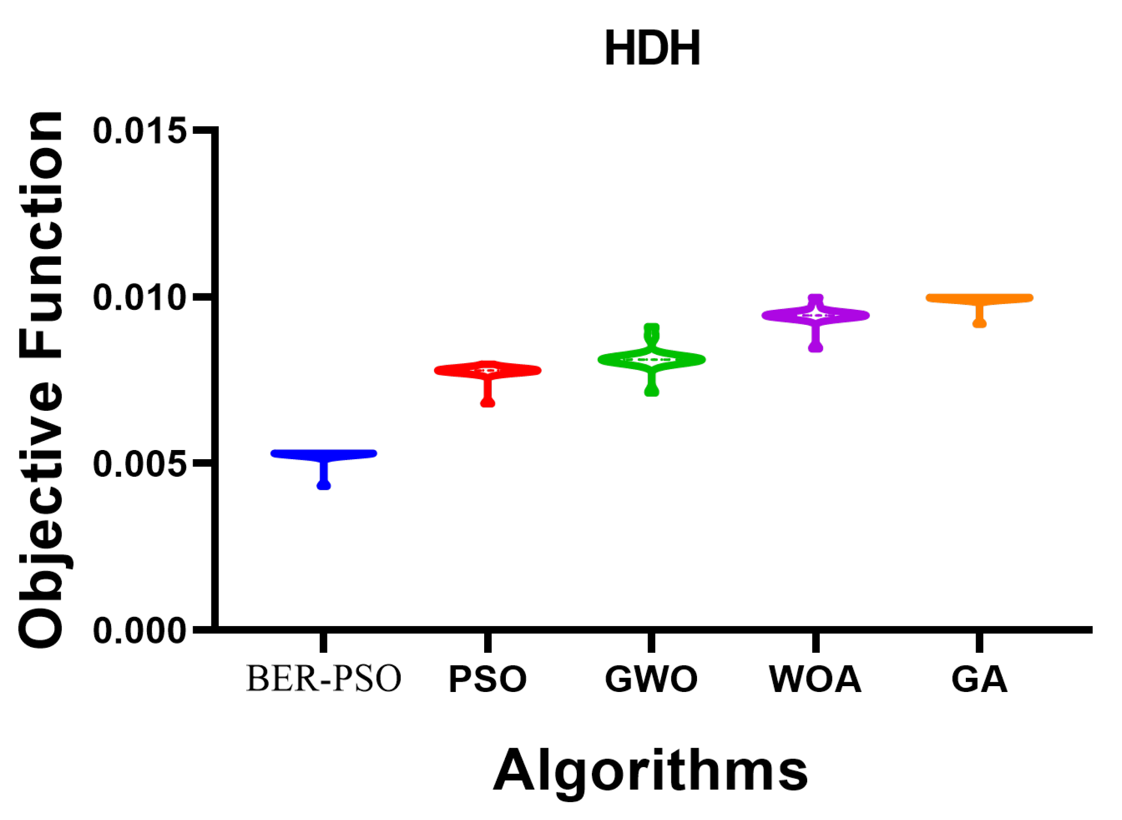
The presented BER–PSO algorithm is also compared with other optimization techniques of PSO [16], GWO [18], WOA [20], and GA [24] algorithms. Figure 3 illustrates the box plot of the presented BER–PSO and compared algorithms for the HDH-tested data. The BER–PSO algorithm shows better results over 16 runs over HDH. While Figure 4 discusses the histogram of the presented BER–PSO and compared algorithms for the HDH-tested data. The BER–PSO algorithm shows better performance over the histogram of HDH.

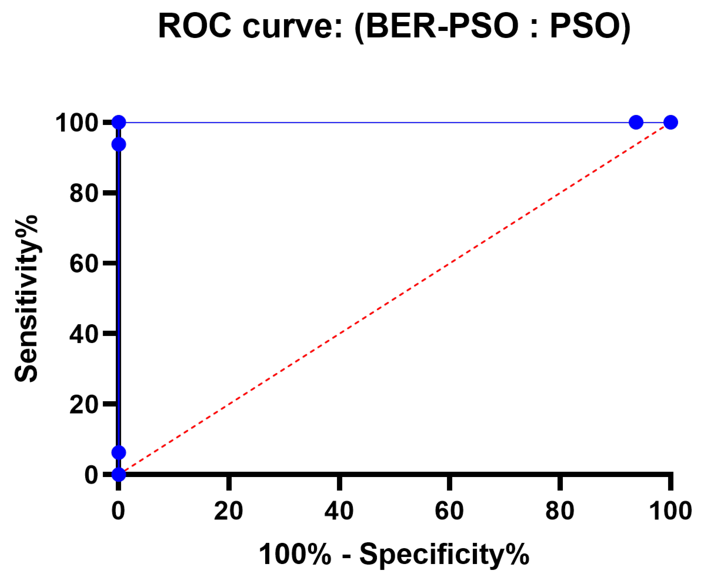
Figure 5 displays the quantile-quantile (QQ) plots as well as the residual plots for the presented BER–PSO method and the algorithms that were compared for the HDH-tested data. The ROC curve of the proposed BER–PSO algorithm compared to the ROC curve of the PSO algorithm for the HDH-tested data is displayed in Figure 6. The performance of the suggested BER–PSO algorithm for the HDH-tested data is demonstrated by these statistics, which prove its effectiveness.

In this section, statistical analysis is carried out in order to verify the effectiveness of the BER–PSO algorithm. The descriptive statistics of the provided BER–PSO method and the algorithms that are being compared for the HDH data are presented in

Table 9. Descriptive statistics of the compared methods for the HDH data and the provided BER–PSO algorithm.

	BER–PSO	PSO	GWO	WOA	GA
Number of values	16	16	16	16	16
Minimum	0.004314	0.006789	0.00712	0.00844	0.009178
25% Percentile	0.005314	0.007789	0.00812	0.00944	0.009978
Median	0.005314	0.007789	0.00812	0.00944	0.009978
75% Percentile	0.005314	0.007789	0.00812	0.00944	0.009978
Maximum	0.005314	0.007989	0.00912	0.00999	0.009998
Range	0.001	0.0012	0.002	0.00155	0.00082
Mean	0.005252	0.007739	0.008163	0.009431	0.009929
Std. Deviation	0.00025	0.000258	0.000404	0.000305	0.0002
Std. Error of Mean	6.25 × 10${}^{-5}$	6.46 × 10${}^{-5}$	0.000101	7.61 × 10${}^{-5}$	5.01 × 10${}^{-5}$
Sum	0.08402	0.1238	0.1306	0.1509	0.1589

. The description includes the minimum, median, maximum, mean, and standard (Std.) deviation of the RMSE for the tested data over 16 runs. The results of the ANOVA test for the suggested BER–PSO algorithm in comparison to the other algorithms are presented in

Table 10. Results of an ANOVA test comparing the proposed BER–PSO method against other algorithms.

	SS	DF	MS	F (DFn, DFd)	p Value
Treatment (between columns)	0.000214	4	5.35 × 10${}^{-5}$	F (4, 75) = 628.5	p < 0.0001
Residual (within columns)	6.38 × 10${}^{-6}$	75	8.51 × 10${}^{-8}$	-	-
Total	0.00022	79	-	-	-

. The results of the Wilcoxon Signed Rank Test for the presented BER–PSO algorithm and the algorithms that were compared may be found in

Table 11. Results of the given BER–PSO algorithm and compared algorithms in the Wilcoxon Signed Rank Test.

	BER–PSO	PSO	GWO	WOA	GA
Theoretical median	0	0	0	0	0
Actual median	0.005314	0.007789	0.00812	0.00944	0.009978
Number of values	16	16	16	16	16
Wilcoxon Signed Rank Test
Sum of signed ranks (W)	136	136	136	136	136
Sum of positive ranks	136	136	136	136	136
Sum of negative ranks	0	0	0	0	0
p value (two tailed)	<0.0001	<0.0001	<0.0001	<0.0001	<0.0001
Exact or estimate?	Exact	Exact	Exact	Exact	Exact
Significant (alpha = 0.05)?	Yes	Yes	Yes	Yes	Yes
How big is the discrepancy?
Discrepancy	0.005314	0.007789	0.00812	0.00944	0.009978

.

5.2.2. Results and Discussion Using SSF Data

The results based on the proposed BER–PSO algorithm for the SSF test data are discussed in this section. The basic models of DTR, MLP, KNR, SVR, and RFR are tested first. In addition, AVE and EKNR are also tested.

Table 12. Results of the experimental comparison of the basic and ensemble models with the BER–PSO based model for the SSF test data.

Model	MAE	MBE	RMSE	RRMSE%	r	NSE	WI	R2
DTR	0.0533	−0.0029	0.0708	18.4687	0.9522	0.9064	0.8689	0.9066
MLP	0.0445	−0.0010	0.0574	14.9891	0.9688	0.9384	0.8905	0.9385
KNR	0.0252	−0.0046	0.0362	9.4493	0.9880	0.9755	0.9380	0.9761
SVR	0.0362	0.0061	0.0477	12.4410	0.9789	0.9575	0.9109	0.9583
RFR	0.0807	0.0048	0.1040	27.1374	0.8949	0.7980	0.8013	0.8009
AVE	0.0368	0.0005	0.0504	9.4493	0.9773	0.9526	0.9095	0.9551
EKNR	0.0219	−0.0018	0.0305	7.9679	0.9913	0.9826	0.9460	0.9827
BER–PSO	0.0031	0.0003	0.00490	0.9031	0.9997	0.9994	0.9914	0.9994

shows the experimental results of the BER–PSO-based model versus basic and ensemble models for the SSF test data. The presented method achieved an RMSE of (0.00490), which is better than the compared models. The RFR achieved the worst RMSE of (0.1040).

The presented BER–PSO algorithm is also compared with other optimization techniques of PSO, GWO, WOA, and GA algorithms. Figure 7 illustrates the box plot of the presented BER–PSO and compared algorithms for the SSF -tested data. While Figure 8 discusses the histogram of the presented BER–PSO and compared algorithms for the SSF -tested data. The QQ and residual plots of the presented BER–PSO and compared algorithms for the SSF -tested data are shown in Figure 9. Figure 10 shows the ROC curve of the proposed BER–PSO algorithm versus the PSO algorithm for the SSF -tested data.

The Statistical analysis is also performed here to confirm the BER–PSO algorithm’s performance for the SSF data.

Table 13. Descriptive statistics of the compared methods for the SSF data and the provided BER–PSO algorithm.

	BER–PSO	PSO	GWO	WOA	GA
Number of values	16	16	16	16	16
Minimum	0.004698	0.00666	0.00713	0.00915	0.00916
25% Percentile	0.004898	0.00766	0.00813	0.00945	0.00966
Median	0.004898	0.00766	0.00813	0.00945	0.00966
75% Percentile	0.004898	0.00766	0.00813	0.00945	0.00966
Maximum	0.004898	0.00766	0.00913	0.0099	0.00998
Range	0.0002	0.001	0.002	0.00075	0.00082
Mean	0.004879	0.007591	0.008173	0.009478	0.009668
Std. Deviation	5.44 × 10${}^{-5}$	0.00025	0.000403	0.000157	0.000172
Std. Error of Mean	1.36 × 10${}^{-5}$	6.24 × 10${}^{-5}$	0.000101	3.93 × 10${}^{-5}$	4.29 × 10${}^{-5}$
Sum	0.07807	0.1215	0.1308	0.1517	0.1547

presents the descriptive statistics of the presented BER–PSO algorithm and the compared algorithms for the SSF data. The description includes the minimum, median, maximum, mean, and standard (Std.) deviation of the RMSE for the tested data over 16 runs.

Table 14. Results of the ANOVA test comparing the presented BER–PSO algorithm against other algorithms for the SSF data.

	SS	DF	MS	F (DFn, DFd)	p Value
Treatment (between columns)	0.000238	4	5.96 × 10${}^{-5}$	F (4, 75) = 1057	p < 0.0001
Residual (within columns)	4.23 × 10${}^{-6}$	75	5.64 × 10${}^{-8}$	-	-
Total	0.000243	79	-	-	-

shows the ANOVA test results of the proposed BER–PSO algorithm versus compared algorithms. Finally,

Table 15. Results of the Wilcoxon Signed Rank Test for the SSF data using the provided BER–PSO algorithm and comparative algorithms.

	BER–PSO	PSO	GWO	WOA	GA
Theoretical median	0	0	0	0	0
Actual median	0.004898	0.00766	0.00813	0.00945	0.00966
Number of values	16	16	16	16	16
Wilcoxon Signed Rank Test
Sum of signed ranks (W)	136	136	136	136	136
Sum of positive ranks	136	136	136	136	136
Sum of negative ranks	0	0	0	0	0
p value (two tailed)	<0.0001	<0.0001	<0.0001	<0.0001	<0.0001
Exact or estimate?	Exact	Exact	Exact	Exact	Exact
Significant (alpha = 0.05)?	Yes	Yes	Yes	Yes	Yes
How big is the discrepancy?
Discrepancy	0.004898	0.00766	0.00813	0.00945	0.00966

presents the Wilcoxon Signed Rank Test results of the presented BER–PSO algorithm and compared algorithms.

6. Conclusions and Future Work

This work employed an improved prediction method based on a supervised machine-learning algorithm to forecast the performance of a hybrid solar desalination system. The proposed algorithm is based on the Al-Biruni Earth Radius (BER) and Particle Swarm Optimization (PSO) algorithms. The BER–PSO algorithm was trained and assessed using experimental data. The outcomes demonstrated the BER–PSO method’s excellent capacity to pinpoint the nonlinear relationship between process responses and operating conditions. Additionally, in comparison to the other models under consideration, it provided higher statistical performance measures for the forecasting of pressure drop values and outlet temperatures for hot and cold fluids. The findings of many algorithms were compared to decide which was the most accurate.

References

1. Abujazar, M.S.S.; Fatihah, S.; Ibrahim, I.A.; Kabeel, A.; Sharil, S. Productivity modelling of a developed inclined stepped solar still system based on actual performance and using a cascaded forward neural network model. J. Clean. Prod. 2018, 170, 147–159. [Google Scholar] [CrossRef]
2. Al-Khudhiri, A.I. Optimal Design of Hybrid MSF/RO Desalination Plant. Master’s Thesis, Department of Chemical Engineering, College of Engineering, Cairo, Egypt, 2006. [Google Scholar]
3. Bacha, H.B.; Damak, T.; Bouzguenda, M.; Maalej, A.Y.; Dhia, H.B. A methodology to design and predict operation of a solar collector for a solar-powered desalination unit using the SMCEC principle. Desalination 2003, 156, 305–313. [Google Scholar] [CrossRef]
4. Wang, X.; Ng, K.C. Experimental investigation of an adsorption desalination plant using low-temperature waste heat. Appl. Therm. Eng. 2005, 25, 2780–2789. [Google Scholar] [CrossRef]
5. Elsheikh, A.H.; Sharshir, S.W.; Elaziz, M.A.; Kabeel, A.; Guilan, W.; Haiou, Z. Modeling of solar energy systems using artificial neural network: A comprehensive review. Sol. Energy 2019, 180, 622–639. [Google Scholar] [CrossRef]
6. Abiodun, O.I.; Jantan, A.; Omolara, A.E.; Dada, K.V.; Mohamed, N.A.; Arshad, H. State-of-the-art in artificial neural network applications: A survey. Heliyon 2018, 4, e00938. [Google Scholar] [CrossRef] [PubMed] [Green Version]
7. Linardatos, P.; Papastefanopoulos, V.; Kotsiantis, S. Explainable AI: A Review of Machine Learning Interpretability Methods. Entropy 2020, 23, 18. [Google Scholar] [CrossRef] [PubMed]
8. El-Kenawy, E.S.M.; Mirjalili, S.; Alassery, F.; Zhang, Y.D.; Eid, M.M.; El-Mashad, S.Y.; Aloyaydi, B.A.; Ibrahim, A.; Abdelhamid, A.A. Novel Meta-Heuristic Algorithm for Feature Selection, Unconstrained Functions and Engineering Problems. IEEE Access 2022, 10, 40536–40555. [Google Scholar] [CrossRef]
9. El-kenawy, E.S.M.; Albalawi, F.; Ward, S.A.; Ghoneim, S.S.M.; Eid, M.M.; Abdelhamid, A.A.; Bailek, N.; Ibrahim, A. Feature Selection and Classification of Transformer Faults Based on Novel Meta-Heuristic Algorithm. Mathematics 2022, 10, 3144. [Google Scholar] [CrossRef]
10. Akinola, O.O.; Ezugwu, A.E.; Agushaka, J.O.; Zitar, R.A.; Abualigah, L. Multiclass feature selection with metaheuristic optimization algorithms: A review. Neural Comput. Appl. 2022, 34, 19751–19790. [Google Scholar] [CrossRef] [PubMed]
11. Trojovská, E.; Dehghani, M. A new human-based metahurestic optimization method based on mimicking cooking training. Sci. Rep. 2022, 12, 14861. [Google Scholar] [CrossRef]
12. El-Kenawy, E.S.M.; Mirjalili, S.; Abdelhamid, A.A.; Ibrahim, A.; Khodadadi, N.; Eid, M.M. Meta-Heuristic Optimization and Keystroke Dynamics for Authentication of Smartphone Users. Mathematics 2022, 10, 2912. [Google Scholar] [CrossRef]
13. Alhussan, A.A.; Khafaga, D.S.; El-Kenawy, E.S.M.; Ibrahim, A.; Eid, M.M.; Abdelhamid, A.A. Pothole and Plain Road Classification Using Adaptive Mutation Dipper Throated Optimization and Transfer Learning for Self Driving Cars. IEEE Access 2022, 10, 84188–84211. [Google Scholar] [CrossRef]
14. Abdelhamid, A.A.; El-Kenawy, E.S.M.; Alotaibi, B.; Amer, G.M.; Abdelkader, M.Y.; Ibrahim, A.; Eid, M.M. Robust Speech Emotion Recognition Using CNN + LSTM Based on Stochastic Fractal Search Optimization Algorithm. IEEE Access 2022, 10, 49265–49284. [Google Scholar] [CrossRef]
15. El-kenawy, E.S.M.; Abdelhamid, A.A.; Ibrahim, A.; Mirjalili, S.; Khodadad, N.; Al duailij, M.A.; Alhussan, A.A.; Khafaga, D.S. Al-Biruni Earth Radius (BER) Metaheuristic Search Optimization Algorithm. Comput. Syst. Sci. Eng. 2023, 45, 1917–1934. [Google Scholar] [CrossRef]
16. Bello, R.; Gomez, Y.; Nowe, A.; Garcia, M.M. Two-Step Particle Swarm Optimization to Solve the Feature Selection Problem. In Proceedings of the Seventh International Conference on Intelligent Systems Design and Applications (ISDA 2007), Rio de Janeiro, Brazil, 20–24 October 2007; pp. 691–696. [Google Scholar] [CrossRef]
17. Kabeel, A.; El-Said, E.M. A hybrid solar desalination system of air humidification, dehumidification and water flashing evaporation: Part II. Experimental investigation. Desalination 2014, 341, 50–60. [Google Scholar] [CrossRef]
18. Al-Tashi, Q.; Abdul Kadir, S.J.; Rais, H.M.; Mirjalili, S.; Alhussian, H. Binary Optimization Using Hybrid Grey Wolf Optimization for Feature Selection. IEEE Access 2019, 7, 39496–39508. [Google Scholar] [CrossRef]
19. Şenel, F.A.; Gokçe, F.; Yuksel, A.S.; Yigit, T. A novel hybrid PSO–GWO algorithm for optimization problems. Eng. Comput. 2019, 35, 1359–1373. [Google Scholar] [CrossRef]
20. Mirjalili, S.; Lewis, A. The Whale Optimization Algorithm. Adv. Eng. Softw. 2016, 95, 51–67. [Google Scholar] [CrossRef]
21. Simon, D. Biogeography-Based Optimization. IEEE Trans. Evol. Comput. 2008, 12, 702–713. [Google Scholar] [CrossRef]
22. Samareh Moosavi, S.H.; Khatibi Bardsiri, V. Satin Bowerbird Optimizer. Eng. Appl. Artif. Intell. 2017, 60, 1–15. [Google Scholar] [CrossRef]
23. Fister, I.; Yang, X.S.; Fister, I.; Brest, J. Memetic firefly algorithm for combinatorial optimization. arXiv 2012, arXiv:1204.5165. [Google Scholar]
24. Kabir, M.M.; Shahjahan, M.; Murase, K. A new local search based hybrid genetic algorithm for feature selection. Neurocomputing 2011, 74, 2914–2928. [Google Scholar] [CrossRef]
25. Karakonstantis, I.; Vlachos, A. Bat algorithm applied to continuous constrained optimization problems. J. Inf. Optim. Sci. 2020, 42, 57–75. [Google Scholar] [CrossRef]
26. Breiman, L. Random Forests. Mach. Learn. 2001, 45, 5–32. [Google Scholar] [CrossRef] [Green Version]
27. El-kenawy, E.S.M.; Mirjalili, S.; Ghoneim, S.S.M.; Eid, M.M.; El-Said, M.; Khan, Z.S.; Ibrahim, A. Advanced Ensemble Model for Solar Radiation Forecasting using Sine Cosine Algorithm and Newton’s Laws. IEEE Access 2021, 9, 115750–115765. [Google Scholar] [CrossRef]
28. Jang, S.; Jang, Y.E.; Kim, Y.J.; Yu, H. Input initialization for inversion of neural networks using k-nearest neighbor approach. Inf. Sci. 2020, 519, 229–242. [Google Scholar] [CrossRef]
29. Tharwat, A. Parameter investigation of support vector machine classifier with kernel functions. Knowl. Inf. Syst. 2019, 61, 1269–1302. [Google Scholar] [CrossRef]
30. Noi, P.T.; Kappas, M. Comparison of Random Forest, k-Nearest Neighbor, and Support Vector Machine Classifiers for Land Cover Classification Using Sentinel-2 Imagery. Sensors 2017, 18, 18. [Google Scholar] [CrossRef] [Green Version]
31. El-Said, E.M.; Elaziz, M.A.; Elsheikh, A.H. Machine learning algorithms for improving the prediction of air injection effect on the thermohydraulic performance of shell and tube heat exchanger. Appl. Therm. Eng. 2021, 185, 116471. [Google Scholar] [CrossRef]
32. Kabeel, A.; El-Said, E.M. A hybrid solar desalination system of air humidification dehumidification and water flashing evaporation: A comparison among different configurations. Desalination 2013, 330, 79–89. [Google Scholar] [CrossRef]
33. Pandey, A.; Kumar, R.R.; B, K.; Laghari, I.A.; Samykano, M.; Kothari, R.; Abusorrah, A.M.; Sharma, K.; Tyagi, V. Utilization of solar energy for wastewater treatment: Challenges and progressive research trends. J. Environ. Manag. 2021, 297, 113300. [Google Scholar] [CrossRef]
34. Rashidi, S.; Karimi, N.; Yan, W.M. Applications of machine learning techniques in performance evaluation of solar desalination system—A concise review. Eng. Anal. Bound. Elem. 2022, 144, 399–408. [Google Scholar] [CrossRef]
35. Kumar, R.R.; Pandey, A.; Samykano, M.; Aljafari, B.; Ma, Z.; Bhattacharyya, S.; Goel, V.; Ali, I.; Kothari, R.; Tyagi, V. Phase change materials integrated solar desalination system: An innovative approach for sustainable and clean water production and storage. Renew. Sustain. Energy Rev. 2022, 165, 112611. [Google Scholar] [CrossRef]
36. Gwon, H.; Ahn, I.; Kim, Y.; Kang, H.J.; Seo, H.; Cho, H.N.; Choi, H.; Jun, T.J.; Kim, Y.H. Self–Training With Quantile Errors for Multivariate Missing Data Imputation for Regression Problems in Electronic Medical Records: Algorithm Development Study. JMIR Public Health Surveill. 2021, 7, e30824. [Google Scholar] [CrossRef]
37. Ibrahim, A.; Mirjalili, S.; El-Said, M.; Ghoneim, S.S.M.; Al-Harthi, M.M.; Ibrahim, T.F.; El-Kenawy, E.S.M. Wind Speed Ensemble Forecasting Based on Deep Learning Using Adaptive Dynamic Optimization Algorithm. IEEE Access 2021, 9, 125787–125804. [Google Scholar] [CrossRef]
38. Kalantari, S.; Motameni, H.; Akbari, E.; Rabbani, M. Optimal components selection based on fuzzy-intra coupling density for component-based software systems under build-or-buy scheme. Complex Intell. Syst. 2021, 7, 3111–3134. [Google Scholar] [CrossRef]
39. Emary, E.; Zawbaa, H.M.; Hassanien, A.E. Binary grey wolf optimization approaches for feature selection. Neurocomputing 2016, 172, 371–381. [Google Scholar] [CrossRef]
Figure 1. HDH-SSF experimental setup schematic diagram. F (Flow meter), T (Thermocouple), S (Pyrometer), H (Thermo hygrometer), V (Valve), P (Pump), LI (Level indicator), MT (Mixing Tank), TK (Tank), EH (Electric Heater), SV (Solenoid), SWH (Solar Water Heater), SAH (Solar Air Heater), HHEX (Helical Heat Exchanger), FC (Flashing Chamber), C1 (Condenser), and C2 (Dehumidifier).
Energies 16 01185 g001
Figure 2. The given bBER–PSO and comparable algorithms are depicted in a box plot over the average error metric.
Energies 16 01185 g002
Figure 3. For the HDH tested data, a box plot of the offered BER–PSO and comparing algorithms.
Energies 16 01185 g003
Figure 4. For the HDH-tested data, a histogram of the offered BER–PSO and comparing algorithms is shown.
Energies 16 01185 g004
Figure 5. BER–PSO and comparable methods for the HDH-tested data are provided in QQ and residual plots for the HDH-tested data.
Energies 16 01185 g005
Figure 6. ROC curve comparing the PSO algorithm and the provided BER–PSO algorithm for the HDH testing data.
Energies 16 01185 g006
Figure 7. For the SSF tested data, a box plot of the offered BER–PSO and comparing algorithms.
Energies 16 01185 g007
Figure 8. For the SSF tested data, a histogram of the offered BER–PSO and comparing algorithms is shown.
Energies 16 01185 g008
Figure 9. BER–PSO and comparable methods for the SSF tested data are provided in QQ and residual plots.
Energies 16 01185 g009
Figure 10. ROC curve comparing the PSO algorithm and the provided BER–PSO algorithm for the SSF testing data.
Energies 16 01185 g010