Reinforcement Learning: Theory and Applications in HEMS

Abstract

The steep rise in reinforcement learning (RL) in various applications in energy as well as the penetration of home automation in recent years are the motivation for this article. It surveys the use of RL in various home energy management system (HEMS) applications. There is a focus on deep neural network (DNN) models in RL. The article provides an overview of reinforcement learning. This is followed with discussions on state-of-the-art methods for value, policy, and actor–critic methods in deep reinforcement learning (DRL). In order to make the published literature in reinforcement learning more accessible to the HEMS community, verbal descriptions are accompanied with explanatory figures as well as mathematical expressions using standard machine learning terminology. Next, a detailed survey of how reinforcement learning is used in different HEMS domains is described. The survey also considers what kind of reinforcement learning algorithms are used in each HEMS application. It suggests that research in this direction is still in its infancy. Lastly, the article proposes four performance metrics to evaluate RL methods.

1. Introduction

The largest group of consumers of electricity in the US are residential units. In the year 2020, this sector alone accounted for approximately 40% of all electricity usage [1]. The average daily residential consumption of electricity is 12 kWh per person [2]. Therefore, effectively managing the usage of electricity in homes, while maintaining acceptable comfort levels, is vital to address the global challenges of dwindling natural resources and climate change. Rapid technological advances have now made home energy management systems (HEMS) an attainable goal that is worth pursuing. HEMS consist of automation technologies that can respond to a continuously or periodically changing home environmental as well as relevant external conditions, without human intervention [3,4]. In this review, the term ‘home’ is taken in a broad context to also include all residential units, classrooms, apartments, offices complexes, and other buildings in the smart grid [5,6,7,8].

Artificial Intelligence (AI), more specifically machine learning, is one of the key contributing factors that have helped realize HEMS today [9,10,11]. Reinforcement learning (RL) is a class of machine learning algorithms that is making deep inroads in various applications in HEMS. This learning paradigm incorporates the twin capabilities of learning from experience and learning at higher levels of abstraction. It allows algorithmic agents to replace human beings in the real world, including in homes and buildings, in applications that had hitherto been considered to be beyond today’s capabilities.

RL allows an algorithmic entity to make sequences of decisions and implement actions from experience in the same manner as a human being [12,13,14,15,16,17]. DNN has proven to be a powerful tool in RL, for it endows the RL agent with the capability to adapt to a wide variety of complex real-world applications [18,19]. Moreover, it has been proposed in [20] that RL can attain the ultimate goal of artificial general intelligence [21].

Consequently, RL is making deep inroads into many application domains today. It has been applied extensively to robotics [22]. Specific applications in this area include robotic manipulation with many degrees of freedom [23,24] and the navigation and path planning of mobile robots and UAVs [25,26,27]. RL finds widespread applications in communications and networking [28,29,30]. It has been used in 5G-enabled UAVs with cognitive capabilities [31], cybersecurity [32,33,34], and edge computing [35]. In intelligent transportation systems, RL is used in a range of applications such as vehicle dispatching in online ride-hailing platforms [36].

Other domains where RL has been used include hospital decision making [37], precision agriculture [38], and fluid mechanics [39]. The financial industry is another important sector where RL has been adopted for several scenarios [40,41,42]. It is of little surprise that RL has been extensively used to solve various problems in energy systems [43,44,45,46,47]. Another review article on the use of RL [47] considers three application areas in frequency and voltage control as well as in energy management.

RL is increasingly being used in HEMS applications and several review papers have already been published. The review article in [48] focuses on RL for HVAC and water heaters. The paper in [49] is based on research published between 1997 and 2019. The survey observes that only 11% of published research reports the deployment of RL in actual HEMS. The article in [50] specifically focuses on occupant comfort in residences and offices. A more recent review on building energy management [51] focuses on deep neural network-based RL. A recent article [52] considers RL along with model predictive control in smart building applications. The article in [53] is a survey of RL in demand response.

In contrast to the previous reviews, the scope of our review is broad enough to cover all areas of HEMS, including HEMS interfacing with the energy grid. More importantly, it provides a comprehensive overview of all major RL methods, providing a sufficient level of explanation for readers’ understanding. Therefore, this article would be of benefit for researchers and practitioners in other areas of the energy systems, and beyond, to acquire a theoretical level understanding of basic RL techniques.

The rest of this article is organized in the following manner. Section 2 addresses the various elements of HEMS in greater detail. Section 3 introduces basic ideas on reinforcement learning. Further details of value-based RL and associated deep architectures are discussed in Section 4, while policy-based and actor–critic architectures—the other class of RL algorithms—are described in Section 5. Section 6 and Section 7 discuss the results of the research survey: while Section 6 focuses on the application of RL, Section 7 is a study on the classes of algorithms that were used. The article concludes in Section 8, where the authors propose four metrics to evaluate the performances of RL algorithms in HEMS.

2. Home Energy Management Systems

HEMS refers to a slew of automation techniques that can respond to continuously or periodically changing the home/building’s internal as well as relevant external conditions, and without the need for human intervention. This section addresses the enabling technologies that make this an attainable goal.

2.1. Networking and Communication

All HEMS devices must have the ability to send/receive data with each other using the same communication protocol. HEMS provides the occupants with the tools that allow them to monitor, manage, and control all the activities within the system. The advancements in technologies and more specifically in IoT-enabled devices and wireless communications protocols such as ZigBee, Wi-Fi, and Z-Wave made HEMS feasible [54,55]. These smart devices are connected through a home area network (HAN) and/or to the internet, i.e., a wide area network (WAN).

The choice of communication protocol for home automation is an open question. To a large extent, it depends on the user’s personal requirements. If it is desired to automate a smaller set of home appliances with ease of installation, and operability in a plug-and-play manner, Wi-Fi is the appropriate one to use. However, with more extensive automation requirements, involving tens through to hundreds of smart devices, Wi-Fi is no longer the optimal choice. There are issues relating to scalability and signal interference in Wi-Fi. More importantly, due to its relatively high energy consumption, Wi-Fi is not appropriate for battery-powered devices.

Under these circumstances, ZigBee and Z-Wave are more appropriate [56]. These communication protocols dominate today’s home automation market. There are many common features shared between the two protocols. Both protocols use RF communication mode and offer two-way communication. Both ZigBee and Z-Wave enjoy well established commercial relationships with various companies, with tens of hundreds of smart devices using one of these protocols.

Z-Wave is superior to than ZigBee in terms of the range of transmission (120 m with three devices as repeaters vs. 60 m with two devices working as repeaters). In terms of inter-brand operability, Z-Wave again holds the advantage. However, ZigBee is more competitive in terms of data rate of transmission as well as in the number of connected devices. Z-Wave was specially created for home automation applications, while ZigBee is used in a wider range of places such as industry, research, health care, and home automation [57]. A study conducted by [58] foresees that ZigBee is most likely to be the standard communication protocol for HEMS. However, due to the presence of numerous factors, it is still difficult to tell with high certainty if this forecast would take place in future. It is also possible that an alternative communication protocol will emerge in future.

HEMS requires this level of connectivity to be able to access electricity price from the smart grid through the smart meter and control all the system’s elements accordingly (e.g., turn on/off the TV, control the thermostat settings, determine the charge/discharge battery timings, etc.). In some scenarios, HEMS uses the forecasted electricity prices to schedule shiftable loads (e.g., washing machine, dryer, electric vehicle charging) [54].

2.2. Sensors and Controller Platforms

HEMS consists of smart appliances with sensors, these IoT-enabled devices communicate with the controller by sending and receiving data. They collect information from the environment and/or about their electricity usage using built-in sensors. The smart meter gathers information regarding the total consumers’ consumption from the appliances, the peak load period, and electricity price from the smart grid.

The controller can be in the form of a physical computer located within the premises, that is equipped with the ability to run complex algorithms. An alternate approach is to leverage any of the cloud services that are available to the consumers through cloud computing firms.

The controller gathers information from the following sources: (i) the energy grid through the smart meter, which includes the power supply status and electricity price, (ii) the status of renewable energy and the energy storage systems, (iii) the electricity usage of each smart device at home, and (iv) the outside environment. Then it processes all the data through a computational algorithm to take specific action for each device in the whole system separately [5].

2.3. Control Algorithms

AI and machine learning methods are making deep inroads into HEMS [10,59]. HEMS algorithms incorporated into the controller might be in the form of simple knowledge-based systems. These approaches embody a set of if-then-else rules, which may be crisp or fuzzy. However, due to their reliance on a fixed set of rules, such methods may not be of much practical use with real-time controllers. Moreover, they cannot effectively leverage the large amount of data available today [5]. Although it is possible to impart a certain degree of trainability to fuzzy systems, the structural bottleneck of consolidating all inputs using only conjunctions (and) and disjunctions (or) still persists.

Numerical optimization comprises of another class of computational methods for the smart home controller. These methods entail an objective function that is to be either minimized (e.g., cost) or maximized (e.g., occupant comfort), as well as a set of constraints imposed by the underlying physical HEMS appliances and limitations. Due to its simplicity, linear programing is a popular choice for this class of algorithms. More recently, game theoretic approaches have emerged as an alternative approach for various HEMS optimization problems [5].

In recent years, artificial intelligence and machine learning, more specifically deep learning techniques, have become popular for HEMS applications. Deep learning takes advantage of all the available data for training the neural network to predict the output and control the connected devices. It is very helpful to forecast the weather, load, and electricity price. Furthermore, it handles non-linearities without resorting to explicit mathematical models. Since 2013, there have been significant efforts directed at using deep neural networks within an RL framework [60,61], that have met with much success.

3. Overview of Reinforcement Learning

3.1. Deep Neural Networks

A deep neural network (DNN) is a trainable highly nonlinear function approximator of the form $y\left(·\right):{\mathcal{R}}^M\to {\mathcal{R}}^N$ where $M$ and $N$ are the dimensionalities of the input and output spaces. Structurally, the DNN consists of an input layer and output layer, and at least one hidden layer. The input layer receives the DNN input vector $x$. The neurons in any other layer receive, as their inputs, the weighted outputs of neurons in the preceding layer. The weights of the DNN make up its weight parameter, denoted $\mathsf{\theta }$. For simplicity, we consider DNNs with scalar outputs so that $y\left(·\right):{\mathcal{R}}^M\to \mathcal{R}$. The actual output of the DNN is represented as $y\left(x|\mathsf{\theta }\right)$, which is that of the sole neuron in the output layer.

In a typical regression application, the DNN’s training set $\mathcal{S}$ consists of pairs $\left(x\left(n\right), t\left(n\right)\right)\in \mathcal{S}$ where $n=1,\dots ,\left|\mathcal{S}\right|$ is the sample index (for the sake of conciseness, this relationship is often denoted as $n\in \mathcal{S}$ in this article). The quantity $t\left(n\right)$ is the target, or desired output. During training, $\mathsf{\theta }$ is updated in steps so that for each input $x\left(n\right)$, the DNN’s output $y\left(n\right)$ is as close as possible to $t\left(n\right)$. Supervised learning algorithms aim to minimize the DNN’s loss function $J_{\mathcal{S}}\left(\mathsf{\theta }\right)$. The subscript $\mathcal{S}$ indicates that the loss is an empirically estimate over the sample in $\mathcal{S}$. A popular choice of the latter is the averaged squared $L_2$ norms of the difference between the target and output for all samples in $\mathcal{S}$,

$$\begin{array}{c}{J}_{\mathcal{S}}\left(\mathsf{\theta }\right)=\frac{1}{2}\frac{1}{\left|\mathcal{S}\right|}{\displaystyle {\displaystyle \sum }_{n\in \mathcal{S}}}{\left(y\left(x\left(n\right)|\mathsf{\theta }\right)-t\left(n\right)\right)}^2\end{array}$$

(1)

Training the DNN comprises of multiple passes called epochs, with each epoch comprising of one pass through all samples in $\mathcal{S}$. In stochastic gradient descent (SGD), with $\eta \ll 1$ being the learning rate, the parameter $\mathsf{\theta }$ is incremented once for every sample $n\in \mathcal{S}$ as,

$$\begin{array}{c}\mathsf{\theta }\leftarrow \mathsf{\theta }-\eta \left(y\left(x\left(n\right)|\mathsf{\theta }\right)-t\left(n\right)\right){\nabla }_{\mathsf{\theta }}y\left(x\left(n\right)|\mathsf{\theta }\right)\end{array}$$

(2)

This increment is equivalent to a single gradient step with $J\left(\mathsf{\theta }\right)=\frac{1}{2}{\left(y\left(x\left(n\right)|\mathsf{\theta }\right)-t\left(n\right)\right)}^2$.

While SGD is useful in many online applications, minibatch gradient descent is the most common training method. In each epoch, $\mathcal{S}$ are divided into non-overlapping minibatches ${\mathcal{B}}_k\subset \mathcal{S}$ (i.e., ${{\displaystyle \mathrm{\cup }}}_k{\mathcal{B}}_k=\mathcal{S}$, and $k\ne l\Rightarrow {\mathcal{B}}_k\cap {\mathcal{B}}_l=\varphi$). The parameter $\mathsf{\theta }$ is updated once for every minibatch $\mathcal{B}$ as,

$$\begin{array}{c}\mathsf{\theta }\leftarrow \mathsf{\theta }-\eta \frac{1}{\left|\mathcal{B}\right|}{\displaystyle {\displaystyle \sum }_{n\in \mathcal{B}}}\left(y\left(x\left(n\right)|\mathsf{\theta }\right)-t\left(n\right)\right){\nabla }_{\mathsf{\theta }}y\left(x\left(n\right)|\mathsf{\theta }\right)\end{array}$$

(3)

One of the advantages of training in minibatches is that the trajectory taken by the training algorithm is straightened out, thereby speeding up convergence. It can be seen that the loss function is $J_{\mathcal{B}}\left(\mathsf{\theta }\right)$, which is identical to that in Equation (1), with sample set $\mathcal{B}$.

Typically, the loss function includes an additional regularization term designed to keep the weights in $\mathsf{\theta }$ low in order to prevent overfitting; overfitting results in poorer performance after the DNN is deployed into the real world. Nowadays, faster training is accomplished by using extensions of gradient descent such as ADAM. These as well as many other important aspects of DNNs and training algorithms have not been addressed here; the above discussion minimally suffices to understand how DNNs are used in reinforcement learning (RL). A brief exposition to DNNs is available at [62]. For a rigorous treatment of DNNs, the interested reader is referred to [63].

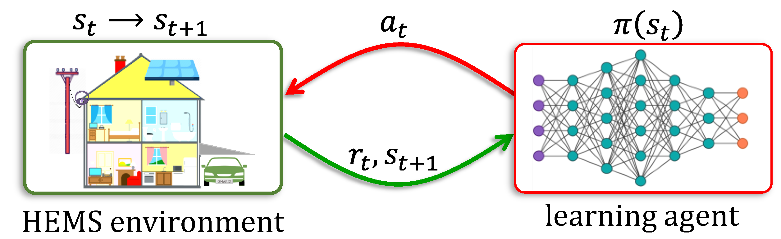
3.2. Reinforcement Learning

An agent in RL is a learning entity, such as a deep neural network (DNN) that exerts control over a stochastic, external environment by means of a sequence of actions over time. The agent learns to improve the performance of its environment using reward signals that it receives from the environment.

Rewards are quantitative metrics that indicate the immediate performance of the environment (e.g., average instantaneous user comfort). The sets $\mathbb{S}$ and $\mathbb{A}$ are the state and action spaces and can be discrete or continuous. Everywhere in this article it is assumed that all temporal signals are sampled at discrete, regularly spaced intervals [62]. At each discrete time instance $t$, the current state $s_t\in \mathbb{S}$ of the environment is known to the agent, which then implements an action $a_t\in \mathbb{A}$. The environment transitions to the next state $s_{t+1}$ with a probability $p\left(s_{t+1}|s_t,a_t\right)$ while returning an immediate reward signal $r_t\equiv r\left(s_t,a_t,s_{t+1}\right)$; where $r\left(·\right):\mathbb{S}\times \mathbb{A}\times \mathbb{S}\to \mathcal{R}$ denotes the environment’s reward function that it unknown to the agent. The transition can be denoted concisely as $s_t\stackrel{a_t,r_t}{\to }{s}_{t+1}.$ The overall schematic is shown in Figure 1.

Instead of greedily aiming to improve the immediate reward $r_t$ at every time instance $t$, the agent may be iteratively trained to maximize the sum of the immediate and the weighted future rewards, which is called the return,

$$\begin{array}{c}{R}_t=r_t+{\displaystyle {\displaystyle \sum }_{t^{\prime }=1}^{T-t}}{\gamma }^{t^{\prime }}{r}_{t+t^{\prime }}\end{array}$$

(4)

The quantity $\gamma \in \left[0,1\right]$ is called the discount factor. This lookahead feature prevents the agent to learn greedy actions that fetch large instantaneous rewards, $r_t$ at each instant $t$, while adversely affect the environment later on. The process begins at time $t=0$ and terminates at time $t=T$, the time horizon. The environment’s initial state at $t=0$ is denoted as $s_0\in \mathbb{S}$. The initial state may be probabilistic, following a distribution $p_0$. It should be noted that if $T=\infty$, then the discount must be less than unity ($\gamma <1$) so that the return $R_t$ stays finitely bounded at all times $t$.

The 5-tuple $\left(\mathbb{S},\mathbb{A},p,r,\gamma \right)$ defines a Markov decision process (MDP). The initial state distribution $p_0$ is assumed to be subsumed by the transition probabilities $p$. The MDP can be viewed as an extension of a discrete Markov model.

The entire sequence of states, actions, and rewards is an episode, denoted $\mathcal{E}$, so that,

$$\begin{array}{c}\mathcal{E}\equiv s_0\stackrel{a_0,r_0}{\to }{s}_1\stackrel{a_1,r_1}{\to }{s}_2\cdots \stackrel{a_{T-1},r_{T-1}}{\to }{s}_T\end{array}$$

(5)

The policy can be deterministic or stochastic. A deterministic policy can be treated as a function $\pi :\mathbb{S}\to \mathbb{A}$ (see Figure 1) so that $a_t=\pi \left(s_t\right)$, whereas a stochastic policy $\pi$ represents a probability distribution over $\mathbb{A}$ such that $a_t~\pi \left(s_t\right)$. In several domains, the probability distribution is determined from the nature of the application itself.

During an episode, the action taken by the agent is in accordance with a policy $\pi \in \mathsf{\Pi }$, where $\mathsf{\Pi }$ is the policy space. From the Markovian (memoryless) property of the MDP, it follows that the optimal action of an agent at each state in terms of its stated goal of maximizing the total return $R_t$, is independent of all previous states of the environment. Therefore, the action $a_t$ taken by the agent at time $t$ under policy $\pi$ is based solely on the state $s_t$, and the prior history of states and actions need not be taken into account.

The overall aim of reinforcement learning is usually to maximize an objective function $J\left(·\right)$. Let $J\left(\mathcal{E}\right)$ denote the total return $R_0$ of a given episode $\mathcal{E}$. If the MDP is initialized to any state $s\in \mathbb{S}$ at $t=0$ (such that $s_0=s$), the expected value of this return which is dependent on policy $\pi$ may be expressed as,

$$\begin{array}{c}{J}^{\pi }\left(s\right)={\mathbb{E}}_{\pi }\left[\left.R_0\right|s_0=s\right]\end{array}$$

(6)

The operator ${\mathbb{E}}_{\pi }\left[\mathrm{\Delta }\right]$ is the expectation when all episodes are generated by the MDP under policy $\pi$. When it follows the MDP’s initial state distribution, i.e., $s_0~p$, the expectation may be denoted simply as $J^{\pi }$ without any argument. This informal function overloaded convention is adopted throughout this manuscript as there are other ways to define the objective function. The policy that at each state $s$ implements the action that maximize $J^{\pi }\left(s\right)$ is referred to as the optimal policy and represented as ${\pi }^{\ast }$.

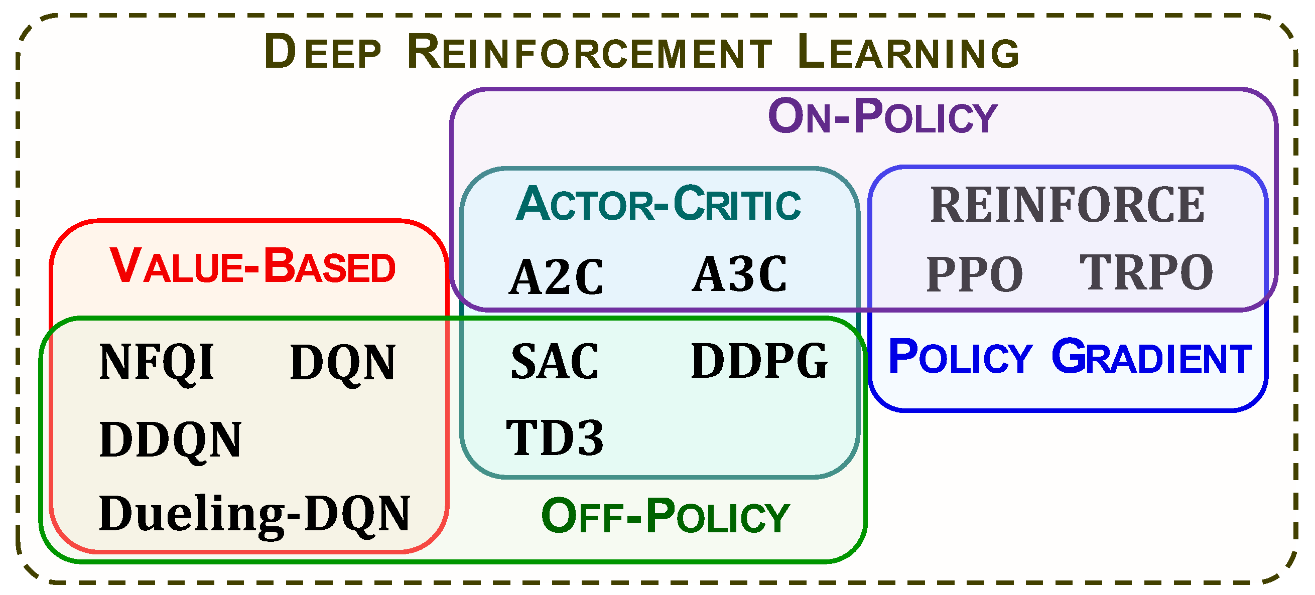
3.3. Taxonomy of Algorithms

RL methods can be classified in several ways. In model-free training, RL takes place with the agent connected to the real-world environment, whereas in model-based RL, the agent is trained using a simulation platform to represent the environment.

In model-based RL, as the transition probabilities and the reward function are available through the environmental model platform, the algorithm must be implemented in an offline manner. Of more practical interest is online RL where the agent can be trained in real time by interacting with the real physical environment as shown in Figure 1. Although online RL is considered to be model-free, practically all research papers report the use of HEMS models for training [49].

In on-policy RL, a referential policy ${\pi }^{\ast }$, such as that of a human, is considered to be the optimal policy and is known a priori. The goal of RL is to learn a policy $\pi \cong {\pi }^{\ast }$. In off-policy approaches, the goal is to obtain the optimal policy ${\pi }^{\ast }$, which maximizes $J^{\pi }\left(s\right)$ in Equation (6).

Another fundamental trichotomy of the plethora of RL approaches used today includes value-based RL, policy-based RL, and actor–critic RL, the latter having emerged more recently. Actor–critic methods are hybrid approaches that borrow features from value-based as well as policy-based RL [64]. The classification of various approaches used in HEMS applications is shown in Figure 2. These are also described at great length in this article, which may be used as a tutorial style exposition to RL for the interested reader.

4. Value-Based Reinforcement Learning

Historically value-based RL, first proposed in [65], heralds the advent of the broad area of reinforcement learning as a distinct branch of AI. These approaches are based on dynamic programming. The formal definition of an MDP was introduced shortly thereafter [66,67]. As noted earlier, an MDP is memoryless. An implication of this feature is that when the environment is in any given state $s_t=s$ at any instant $t$, the prior history $s_0\stackrel{a_0,r_0}{\to }{s}_1\stackrel{a_1,r_1}{\to } \cdots \stackrel{a_{t-1},r_{t-1}}{\to }$ is not of any consequence in deciding the future course of actions [19]. Accordingly, one can define the state–action value, or Q-value of the state $s\in \mathbb{S}$ and for each action $a\in \mathbb{A}$, as the expected return when taking $a$ from $s$ (cf. [19]),

$$\begin{array}{c}q\left(s,a\right)\triangleq {\mathbb{E}}_{\pi }\left[\left.R_t\right|s_t=s,a_t=a\right]\end{array}$$

(7)

Referring to a specific policy $\pi$ may be achieved by using a superscript in the above equation, so that the left-hand side of Equation (7) is written as $q^{\pi }\left(s,a\right)$.

It must be noted that even under a deterministic policy, $q^{\pi }\left(s,a\right)$ can still be defined for any action $a\ne \pi \left(s\right)$ merely by treating $a$ as an evaluative action and following the policy at all future times. Whence (cf. [19]),

$$\begin{array}{c}{q}^{\pi }\left(s,a\right)={\displaystyle {\displaystyle \sum }_{s^{\prime }\in \mathbb{S}}}p\left(s^{\prime }|s,a\right)\left(r\left(s,a,s^{\prime }\right)+\gamma {\displaystyle {\displaystyle \sum }_{a^{\prime }\in \mathbb{A}}}\pi \left(a\text{'}|s^{\prime }\right)q^{\pi }\left(s^{\prime },a^{\prime }\right)\right)\end{array}$$

(8)

The Q-value function $q^{\pi }:\mathbb{S}\times \mathbb{A}\to \mathcal{R}$ can be defined using (6) irrespective of whether the policy is stochastic or deterministic. In case of a deterministic policy, Equation (8) can be applied by letting $\pi \left(a\text{'}|s^{\prime }\right)=1$ when $a^{\prime }=\pi \left(s^{\prime }\right)$, and $\pi \left(a\text{'}|s^{\prime }\right)=0$ otherwise.

A stochastic policy is intrinsic to many real-world applications. For instance, in order to decrease the ambient temperature by manually lowering the thermostatic setting, the final setting involves a degree of randomness arising from human imprecision. In multiagent environments, the best course may often be to adopt a stochastic policy. As an example, in a repeated game of rock–paper–scissors, randomly selecting each action (‘rock’, ‘paper’, or ‘scissors’) with equal probabilities of ⅓ is the only policy that would ensure that the probability of losing a round of the game does not exceed that of winning.

From a machine learning standpoint, stochastic policies help explore and assess the effects of the entire repertoire of actions available in $\mathbb{A}$. Such exploration is critical during the initial stages of the learning algorithm. The two most commonly used stochastic policies are the $ϵ$-greedy and the softmax policies. Under an $ϵ$-greedy policy $\pi$, the probability of picking an action $a$ when the environmental state is $s$ is given by,

$$\begin{array}{c}\pi \left(a|s\right)=\left\{\begin{array}{c}\frac{ϵ}{\left|\mathbb{A}\right|}+\left(1-ϵ\right), a=\underset{a^{\prime }\in \mathbb{A}}{\mathrm{argmax}}q\left(s,a^{\prime }\right)\\ \frac{ϵ}{\left|\mathbb{A}\right|} , a\ne \underset{a^{\prime }\in \mathbb{A}}{\mathrm{argmax}}q\left(s,a^{\prime }\right)\end{array}\right.\end{array}$$

(9)

It is always a good idea to lower the parameter $ϵ$ steadily so that as learning progresses, the agent is greedier—being likelier to select actions with the highest Q-values, ${\mathrm{argmax}}_{a^{\prime }}q\left(s,a^{\prime }\right)$. The softmax policy is the other popular method to incorporate exploration into a policy. The probability of applying action $a$ under such a policy $\pi$ is,

$$\begin{array}{c}\pi \left(a|s\right)={\left[{\displaystyle {\displaystyle \sum }_{a^{\prime }\in \mathbb{A}}}{e}^{\frac{q\left(s,a^{\prime }\right)}{\tau }}\right]}^{-1}{e}^{\frac{q\left(s,a\right)}{\tau }}\end{array}$$

(10)

Initialized to a high value, the Gibbs–Boltzmann parameter $\tau$ may be steadily lowered as the learning algorithm progresses, so that the policy becomes increasingly exploitative, that is, taking the action with the highest Q-value more often. Unless specified otherwise, it shall be assumed hereafter that the policy space $\mathsf{\Pi }$ is stochastic so that actions follow probability distribution ($a~\pi \left(s\right)$).

Exploration is applied to stochastically search and evaluate the available repertoire of actions at each state, before converging towards the optimal one. It is an essential component of value-based RL. Since exploitation is the strategy of picking the best actions in $\mathsf{\Pi }$, it should not be applied until the algorithm has all actions in a sufficient manner. However, endowing the learning algorithm with too much exploration slows down the learning. Identifying the right tradeoff between exploration and exploitation is a widely studied problem in machine learning [68]. It is for this reason that the parameters $ϵ$ in Equation (9), and $\tau$ in Equation (10) are steadily lowered as learning progresses.

Instead of an evaluative action $a$, suppose the policy $\pi$ is applied from state $s$ (so that either $a=\pi \left(s\right)$ or $a~\pi \left(s\right)$), then the expected return is called the state’s value,

$$\begin{array}{c}v\left(s\right)\triangleq {\mathbb{E}}_{\pi }\left[\left.R_t\right|s_t=s\right]\end{array}$$

(11)

As with the Q-value function, the policy $\pi$ becomes explicit if the value of $s$ is written as $v^{\pi }\left(s\right)$. The value of $s$ can be expressed in terms of Q-values as,

$$\begin{array}{c}v\left(s\right)\equiv {\displaystyle {\displaystyle \sum }_a}\pi \left(a|s\right)q^{\pi }\left(s,a\right)={\mathbb{E}}_{a~\pi \left(s\right)}\left[q^{\pi }\left(s,a\right)\right]\end{array}$$

(12)

The difference between value of any state $s$ and the Q-value of implementing an action $a$ from $s$ under policy is the advantage function, so that,

$$\begin{array}{c}{A}^{\pi }\left(s\right)\equiv q^{\pi }\left(s,a\right)-v^{\pi }\left(s\right)\end{array}$$

(13)

Although the preferred notation in this manuscript is to use lowercase letters to denote variables, the advantage function is represented using uppercase as the lowercase $a$ is reserved to denote an action.

The value function $v:\mathbb{S}\to \mathcal{R}$ allows the optimal policy ${\pi }^{\ast }$ to be defined in a formal manner. If the objective function with the MDP initialized to some $s_0\in \mathbb{S}$ is defined as in Equation (6), then it is evident from Equation (10) that $J^{\pi }\left(s_0\right)=v\left(s_0\right)$. Furthermore, if the MDP visits state $s_t=s$ at the instant $t$, then from Equation (4),

$$\begin{array}{c}{\mathbb{E}}_{\pi }\left[R_0\right]=r_0+\gamma r_1+\dots +{\gamma }^{t-1}{r}_{t-1}+{\gamma }^t{v}^{\pi }\left(s\right)\end{array}$$

(14)

At this stage, we invoke the memoryless property of the underlying MDP. At instant $t$ the partial sum of the terms $r_0+\gamma r_1+\dots +{\gamma }^{t-1}{r}_{t-1}$ in the right-hand side are part of the episode’s history, while ${\gamma }^t{v}^{\pi }\left(s\right)$ is the expected future return. The optimal policy at every such state $s$ is to implement the action that maximizes $v^{\pi }\left(s\right)$, so that,

$$\begin{array}{c}{\pi }^{\ast }\left(s\right)\triangleq \underset{\pi \in \mathsf{\Pi }}{\mathrm{argmax}} v^{\pi }\left(s\right)\end{array}$$

(15)

When the policy ${\pi }^{\ast }$ is deterministic, it can also be inferred that the optimal action from state $s$ is to select the action with the highest Q-value. From Equation (15) it follows that,

$$\begin{array}{c}{a}^{\ast }\triangleq \underset{a\in \mathbb{A}}{\mathrm{argmax}} q^{\ast }\left(s,a\right)\end{array}$$

(16)

The Q-value $q^{\ast }\left(s,a\right)$ is equal to $q^{{\pi }^{\ast }}\left(s,a\right)$. It can be mathematically established that the Q-values corresponding to the optimal policy are higher than those associated with other policies, i.e., $q^{\ast }\left(s,a\right)\ge q^{\pi }\left(s,a\right)$ [69].

The Bellman’s equation for optimality follows from the above consideration,

$$\begin{array}{c}{q}^{\ast }\left(s,a\right)={\displaystyle {\displaystyle \sum }_{s^{\prime }\in \mathbb{S}}}p\left(s^{\prime }|s,a\right)\left(r\left(s,a,s^{\prime }\right)+\gamma \underset{a^{\prime }\in \mathbb{A}}{ \max }{q}^{\ast }\left(s^{\prime },a^{\prime }\right)\right)\end{array}$$

(17)

The difference between Equation (8) and Equation (17) is in the second term in each summand. The policy-based Q-value in Equation (8) is replaced with the maximum Q-value in Equation (17). A mathematically rigorous coverage of various RL methods can be found in the seminal book [70] that is available online.

4.1. Tabular Q-Learning

The simplest possible implementation of the Q-learning algorithm is tabular Q-learning where an $\left|\mathbb{S}\right|\times \left|\mathbb{A}\right|$ sized array is maintained to store $q\left(s,a\right)$ for every state–action pair [71]. Initialized to either zeros or small random values, the tabular entries are periodically updated. As it is an online approach, Q-learning cannot use transition probabilities $p\left(s^{\prime }|s,a\right)$. For each transition $s\stackrel{a,r}{\to }{s}^{\prime }$, the tabular entry for $q\left(s,a\right)$ is incremented as,

$$\begin{array}{c}q\left(s,a\right)\leftarrow \left(1-\eta \right)q\left(s,a\right)+\eta t\end{array}$$

(18)

The quantity $\eta$ is the learning rate; usually $\eta \ll 1$. The quantity $t$ is the target,

$$\begin{array}{c}t=r+\gamma \underset{a^{\prime }\in \mathbb{A}}{ \max }q\left(s^{\prime },a^{\prime }\right)\end{array}$$

(19)

In order to impart an exploratory component to Q-learning, the action $a$ must be selected probabilistically as in Equation (9) or Equation (10). In many cases, increments are applied in real time at the end of each time instance. It can be shown mathematically that the tabular entries converge towards the maximum values, $q^{\ast }\left(s,a\right)$ [69], implying that Q-learning is an off-policy approach. The fully trained agent can select actions as per Equation (16) during actual use.

SARSA (State–Action–Reward–State–Action) [70,72] is the on-policy RL algorithm that can be implemented in a tabular manner. The update rule for SARSA is identical to the earlier expression in Equation (19). However, since SARSA is an on-policy algorithm, the target is specific to the policy $\pi$ and is given by,

$$\begin{array}{c}t=r+\gamma q\left(s^{\prime },\pi \left(s^{\prime }\right)\right)\end{array}$$

(20)

Both Q-learning and SARSA use the tabular entries $q\left(s^{\prime },a^{\prime }\right)$ of the environment’s new state $s^{\prime }$ following the transition $s\stackrel{a,r}{\to }{s}^{\prime }$. The difference is in how the entries are used. Whereas Q-learning uses the tabular entry corresponding to the action $a^{\prime }$ with the highest $q\left(s^{\prime },a^{\prime }\right)$, SARSA applies the specified policy $\pi$, using $q\left(s^{\prime },a^{\prime }\right)$, the Q-value of the action $a^{\prime }=\pi \left(s^{\prime }\right)$. This difference is analogous to that between Equation (17) and Equation (8).

Tabular Q-learning and SARSA can handle continuous state as well as action spaces by discretizing them into a finite and tractable number of subdivisions. Unfortunately, such tabular learning methods cannot be applied in many large-scale domains. This is because too many discrete levels would make the algorithm computationally too intensive if not outright intractable.

When the state space $\mathbb{S}$ is too large (e.g., $\left|\mathbb{S}\right|\approx 7.73\times {10}^{45}$ in chess), tabular learning becomes prohibitively expensive not only in terms of storage requirements but also in terms of computational time needed by the RL algorithm. DQNs are well equipped to handle such large discrete as well as continuous state spaces [73]. However, $\left|\mathbb{A}\right|$, the cardinality of the action space, must still be tractably small. In a DQN the mapping from every state action pair $\left(s,a\right)$ to its Q-value is carried out by means of a DNN.

In reality, the DNN input is some feature vector $\phi \left(s\right)$ of the state $s$, where $\phi :\mathbb{S}\to {\mathcal{R}}^D$ and $D$ is the dimensionality of the feature space. In the same manner, the action $a$ can be represented in terms of its feature vectors. However, as $\left|\mathbb{A}\right|$ is small, it is assumed that the action $a$ itself is the other input. In practice, a unary encoding scheme may be used to represent actions. For instance, if $\left|\mathbb{A}\right|=4$, the four discrete actions may be encoded as 0001, 0010, 0100, and 1000. Under these circumstances, the actual input to the DNN is $\left(\phi \left(s\right),a\right)$, and its actual output is $y\left(\phi \left(s\right),a|\mathsf{\theta }\right)$. For simplicity we will treat the DNN input as $\left(s,a\right)$ and the output as $q\left(s,a|\mathsf{\theta }\right)$, that is, $\left(s,a\right)\equiv \left(\phi \left(s\right),a\right)$, and $q\left(s,a|\mathsf{\theta }\right)\equiv y\left(\phi \left(s\right),a|\mathsf{\theta }\right)$. The Q-value $q\left(s,a|\mathsf{\theta }\right)$ is conditioned in terms of the weight parameter $\mathsf{\theta }$ in this manner so as to explicitly reflect its dependence on the latter.

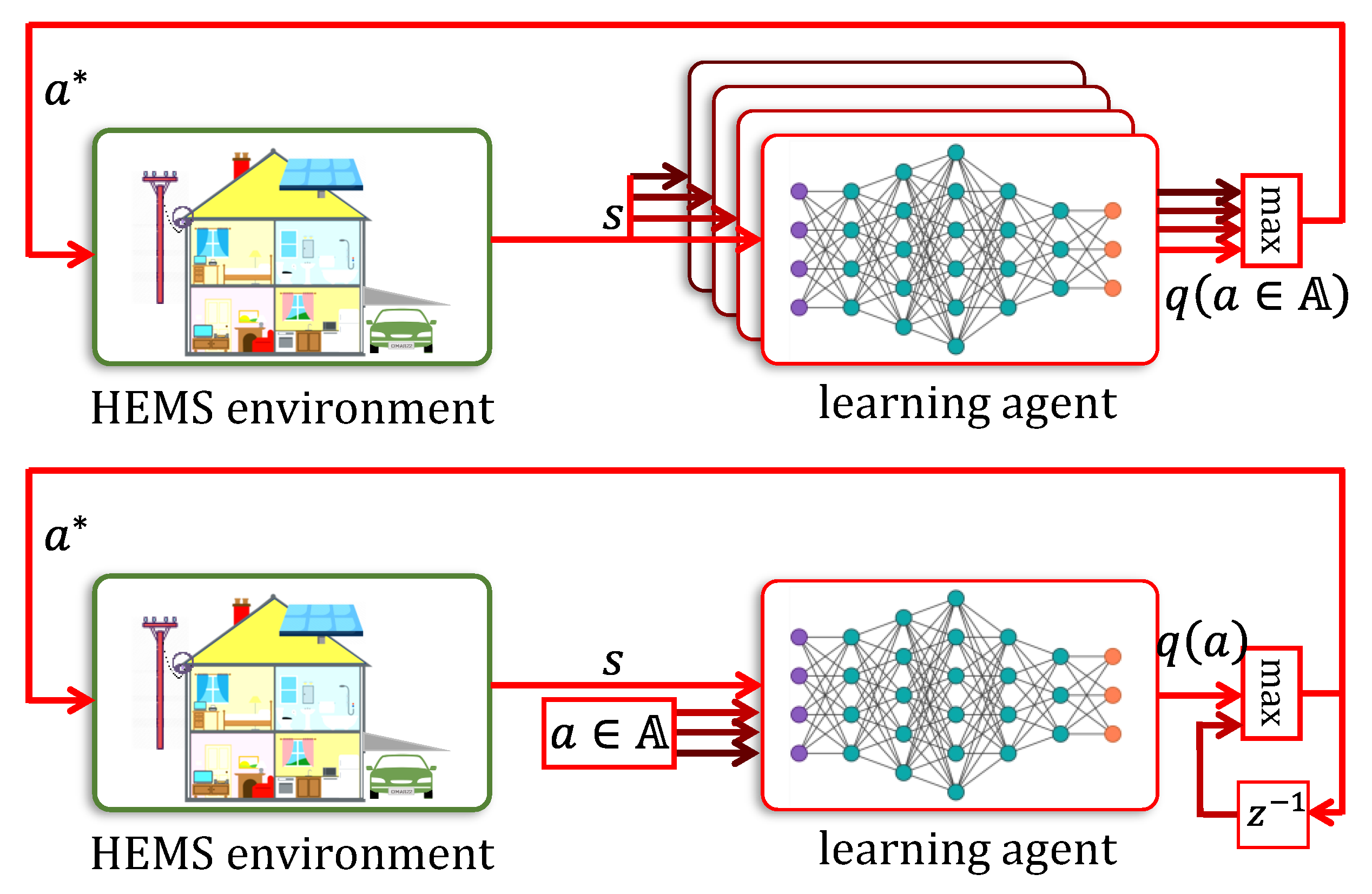
4.2. Deep Q-Networks

There are two possible ways in which the mapping of a state–action pair $\left(s,a\right)$ to its Q-value $q\left(s,a|\mathsf{\theta }\right)$ can be accomplished, which are as follows.

(i)

A different DNN for each action is maintained, so that the total of DNNs in this arrangement is $\left|\mathbb{A}\right|$. The state $s$ (encoded appropriately using the state’s features), serves as the common input to all the DNNs.

(ii)

A single DNN with separate inputs for state $s$ and action $a$ is maintained and its output is $q\left(s,a|\mathsf{\theta }\right)$. While this manner of storing Q-values requires the use of only a single DNN, in order to obtain $\max q\left(s,a|\mathsf{\theta }\right)$, the actions must be applied sequentially to it.

The two schemes are depicted in Figure 3.

Stochastic gradient descent can be applied in a straightforward fashion to train the weight parameter $\mathsf{\theta }$ as in Equation (2) for the squared error loss $\frac{1}{2}{\left(t-q\left(s,a|\mathsf{\theta }\right)\right)}^2$, and with the DNN’s output $y$ now being $q\left(s,a|\mathsf{\theta }\right)$,

$$\begin{array}{c}\mathsf{\theta }\leftarrow \mathsf{\theta }-\eta \left(q\left(s,a|\mathsf{\theta }\right)-t\right){\nabla }_{\mathsf{\theta }}q\left(s,a|\mathsf{\theta }\right)\end{array}$$

(21)

This simple approach is the neural-fitted Q-iteration (NFQI) that was proposed in [74]. The target $t\left(n\right)$ is determined in accordance with Equation (19) with $q\left(s^{\prime },a^{\prime }|\mathsf{\theta }\right)$ used to obtain the target $t$ so that $t=r+\gamma \underset{a^{\prime }\in \mathbb{A}}{ \max }q\left(s^{\prime },a^{\prime }|\mathsf{\theta }\right)$. When using tabular entries in place of $\mathsf{\theta }$, it becomes the fitted Q-iteration (FQI) When the learning agent interacts with the environment, the actions are generally selected using the $ϵ$-greedy method shown in Equation (9).

Temporal correlation in real-time training samples is an unfortunate drawback when directly implementing stochastic gradient descent. Unlike in tabular learning, in DQN updating $\mathsf{\theta }$ changes not only the output $q\left(s,a|\mathsf{\theta }\right)$ for the relevant state–action pair $\left(s,a\right)$ but the Q-values $q\left(s^{\prime },a^{\prime }|\mathsf{\theta }\right)$ of every other pair $\left(s^{\prime },a^{\prime }\right)\ne \left(s,a\right)$ as well. The change may be barely noticeable when $s^{\prime }$ is at a large distance from $s$ within the feature space $\phi \left(\mathbb{S}\right)$; unfortunately, this is not usually the case in most real-world domains.

Consider two successive transitions $s_t\stackrel{a_t,r_t}{\to }{s}_{t+1}\stackrel{a_{t+1},r_{t+1}}{\to }$. Due to the property of temporal correlation between successive states, it is highly reasonable to expect that the distance $\phi \left(s_t\right)-\phi \left(s_{t+1}\right)$ is very small. Therefore, applying Equation (21) to update $q\left(s_t,a_t|\mathsf{\theta }\right)$ will have an undesirable yet pronounced effect on $q\left(s_{t+1},a_{t+1}|\mathsf{\theta }\right)$. A similar argument holds for time sequences of actions as well.

To address the ill effects of temporal correlatedness, DNN training is carried out only after the completion of an episode or multiple episodes, during which time the DQN agent is allowed to exert control over the environment, while $\mathsf{\theta }$ remains unchanged. All training samples are stored in an experience replay buffer $\mathcal{B}$ [75], which plays the role of a mini-batch in DNN training. After enough training samples have been accumulated in $\mathcal{B}$, it is shuffled randomly before incrementing $\mathsf{\theta }$. The increment may be implemented either as in Equation (21), or through minibatch gradient descent as indicated earlier in Equation (3) with $q\left(s,a|\mathsf{\theta }\right)$ replacing $y\left(x|\mathsf{\theta }\right)$ (see Figure 4). For convenience, the update is shown below,

$$\begin{array}{c}\mathsf{\theta }\leftarrow \mathsf{\theta }-\eta \frac{1}{\left|\mathcal{B}\right|}{\displaystyle {\displaystyle \sum }_{n\in \mathcal{B}}}\left(q\left(s\left(n\right),a\left(n\right)|\mathsf{\theta }\right)-t\left(n\right)\right){\nabla }_{\mathsf{\theta }}q\left(s\left(n\right),a\left(n\right)|\mathsf{\theta }\right)\end{array}$$

(22)

The buffer $\mathcal{B}$ is flushed before the next cycle begins with the updated parameter $\mathsf{\theta }$.

An improvement over this scheme is prioritized replay [76], where the probability of a getting selected chosen for a training step is proportional to ${\left(t-q\left(s,a|\mathsf{\theta }\right)\right)}^2+ϵ$. The small constant $ϵ>0$ is added to the squared loss term to ensure that all samples have non-zero probabilities.

Target non-stationarity is another closely related problem that arises in DQNs, one that is not seen in tabular Q-learning. For any given sample transition $s\left(n\right)\stackrel{a\left(n\right),r\left(n\right)}{\to }{s}^{\prime }\left(n\right)$ as the DNN weight parameter $\mathsf{\theta }$ is incremented in accordance with Equation (21), an undesirable effect is that the target $t\left(n\right)$ also changes. This is because the target is determined as $t\left(n\right)=r+\gamma \underset{a^{\prime }\in \mathbb{A}}{ \max }q\left(s^{\prime },a^{\prime }|\mathsf{\theta }\right)$ and this DNN is used to obtain $q\left(s^{\prime }\left(n\right),a^{\prime }|\mathsf{\theta }\right)$. Target non-stationarity is handled by storing an older copy ${\mathsf{\theta }}^{\mathrm{target}}$ of the primary DNN $\mathsf{\theta }$ in memory and using this stored copy to compute the target $t\left(n\right)$. Effectively, the RL algorithm maintains a separate target DNN parametrized by ${\mathsf{\theta }}^{\mathrm{target}}$. Thus, the target is,

$$\begin{array}{c}t\left(n|{\mathsf{\theta }}^{\mathrm{target}}\right)=r\left(n\right)+\gamma \underset{a^{\prime }\in \mathbb{A}}{ \max }q\left(s^{\prime }\left(n\right),a^{\prime }|{\mathsf{\theta }}^{\mathrm{target}}\right)\end{array}$$

(23)

The target DNN’s weight parameter is updated infrequently, and only after $\mathsf{\theta }$ undergoes a significant amount of training. In this manner, the targets remain stationary when training the primary DNN’s parameter $\mathsf{\theta }$ so that gradient descent steps can be implemented in a straightforward manner using terms $\frac{1}{2}{\left(q\left(s\left(n\right),a\left(n\right)|\mathsf{\theta }\right)-t\left(n|{\mathsf{\theta }}^{\mathrm{target}}\right)\right)}^2$ in the loss function $J\left(\mathsf{\theta }\right)$. This scheme is shown in Figure 5.

Overestimation bias [77,78] is another problem frequently encountered in stochastic environments. This is an outcome of maximization. As an example, consider an MDP with $\mathbb{S}=\left\{A,B,C\right\}$ where $C$ is the terminal state. This is shown in Figure 6. The action space $\mathbb{A}=\left\{a_k\right|k=1,2,\dots ,N\}$ where $N$ is relatively large, is available to the agent. From state $A$, only action $a_N$ leads to $B$ whereas the remaining ones, $a_1$ through $a_{N-1}$, lead to $C$. The reward received from state $A$ is always zero, (i.e., $r\left(A,a_k\right)=0$. From state $B$ all actions lead to $C$, with the reward being either $-3$ or $+1$ and with equal probabilities of $N^{-1}$. In other words, the possible transitions are $A\stackrel{a_N,0}{\to }B, A\stackrel{a_{k\ne N},0}{\to }C, B\stackrel{a_k,r\in \left\{-3,1\right\}}{\to }C.$ Since the rewards of $-3$ and 1 have the same probability when the environment transitions from $B$ to $C$, the expected reward from $B$ to $C$ is $-1$ i.e., $\mathbb{E}\left[r\left(B,a_k,C\right)\right]=-1$. For simplicity, let us assume that $\eta =1$. The Q-values for some actions would be updated to $-3$, whereas those of others, to $+1$. Since $N$ is large enough, it is very likely that at least one of them, say $a^{\prime }$ has the higher of the two. Consider the Q-values of actions from state $A$. It is clear that for $k=1$ through $N-1$, $q\left(A,a_k\right)=0$. However, when the agent selects action $a_N$ from $A$, thereby reaching $B$, the operation $\underset{a\in \mathbb{A}}{ \max } q\left(B,a\right)$ is likely to return $+1$ so that $q\left(A,a_N\right)$ would be updated to $\gamma \underset{a\in \mathbb{A}}{ \max } q\left(B,a\right)=\gamma$. This makes $a_N$ appear to be the optimal action from state $A$, when in fact it is the worst choice in $\mathbb{A}$.

Double Q-learning [79] is a popular approach to circumvent overestimation bias in off-policy RL (see Figure 7). Although first proposed in a tabular setting [77], more recent research implements double Q-learning in conjunction with DNNs, which is called the double deep Q-network (DDQN). It incorporates two DNNs with the parameters ${\mathsf{\theta }}^1$ and ${\mathsf{\theta }}^2$. Samples are collected by implementing actions using their mean Q-values, $\frac{1}{2}\left(q\left(s,a|{\mathsf{\theta }}^1\right)+q\left(s,a|{\mathsf{\theta }}^2\right)\right)$. For each sample transition $s\left(n\right)\stackrel{a\left(n\right),r\left(n\right)}{\to }{s}^{\prime }\left(n\right)$ in $\mathcal{B}$ during training, one of the two DNNs, say DNN $j$ ($j\in \left\{1,2\right\}$), is picked randomly and with equal probability to compute the target, and the other DNN, $\overline{j}$ is trained with it. Whence,

$$\begin{array}{c}\left\{\begin{array}{c}t\left(n\right)=r\left(n\right)+\gamma \underset{a^{\prime }\in \mathbb{A}}{ \max }q\left(s^{\prime }\left(n\right),a^{\prime }|{\mathsf{\theta }}^j\right) \\ {\mathsf{\theta }}^{\overline{j}}\leftarrow {\mathsf{\theta }}^{\overline{j}}-\eta {\displaystyle {\displaystyle \sum }_{n\in \mathcal{B}}}\left(q\left(s\left(n\right),a\left(n\right)|{\mathsf{\theta }}^{\overline{j}}\right)-t\left(n\right)\right){\nabla }_{{\mathsf{\theta }}^{\overline{j}}}q\left(s\left(n\right),a\left(n\right)|{\mathsf{\theta }}^{\overline{j}}\right)\end{array}\right.\end{array}$$

(24)

Each DNN has a 0.5 probability of getting trained with the transition sample. This is the manner of updating that was originally proposed in [77].

An extension of DDQN is clipped DDQN [80,81,82]. Instead of selecting the target randomly, it is obtained as minimum of the Q-values, $q\left(s^{\prime }\left(n\right),a^{\prime }|{\mathsf{\theta }}^1\right)$ and $q\left(s^{\prime }\left(n\right),a^{\prime }|{\mathsf{\theta }}^2\right)$,

$$\begin{array}{c}t\left(n\right)=r\left(n\right)+\gamma \underset{j\in \left\{1,2\right\}}{\min }\underset{a^{\prime }\in \mathbb{A}}{ \max }q\left(s^{\prime }\left(n\right),a^{\prime }|{\mathsf{\theta }}^j\right)\end{array}$$

(25)

Dueling DQN architectures (Dueling-DQN) [83] use a different scheme to avoid overestimation bias (see Figure 8). It divides the state–action value $q\left(s,a\right)$ into two parts, the state value $v\left(s\right)$ and the state–action advantage $A\left(s,a\right)$. As shown in Equation (13), $q\left(s,a\right)$ is the difference between the two quantities. The advantage of action $a$ in state $s$, $A\left(s,a\right)$ is the expected gain in the return obtained by picking action $a$. The DNN layout consists of an input layer for the state $s$. After a few initial preprocessing layers, it splits into two separate pathways, each of which is a fully connected DNN. Letting the symbols ${\mathsf{\theta }}^V$ and ${\mathsf{\theta }}^A$ denote the weight parameters of the pathways, the scalar output of the value pathway is the state’s value, $v\left(s|{\mathsf{\theta }}^v\right)$ and the output of the advantage pathway is an $\left|\mathbb{A}\right|$ dimensional vector comprising of the advantages $A\left(s,a|{\mathsf{\theta }}^A\right)$ of all available actions in $\mathbb{A}$. The Q-value of the state–action pair $\left(s,a\right)$ can be obtained in a straightforward manner as provided in the following equation,

$$\begin{array}{c}q\left(s,a|\mathsf{\theta }\right)=v\left(s|{\mathsf{\theta }}^v\right)-{\left|\mathbb{A}\right|}^{-1}{\displaystyle {\displaystyle \sum }_{a^{\prime }}}A\left(s,a^{\prime }|{\mathsf{\theta }}^A\right)\end{array}$$

(26)

The quantity $\mathsf{\theta }$ denotes the set of all weight parameters of the dueling-DQN, including ${\mathsf{\theta }}^V$ and ${\mathsf{\theta }}^A$ as well as those present in the earlier preprocessing layers.

5. Policy-Based and Actor–Critic Reinforcement Learning

Like tabular Q-learning, tabular policy-based RL uses an array of Q-values. Initialized with an arbitrary policy $\pi$, the tabular policy RL algorithm is an iterative process comprising of two steps [70,84]. Policy evaluation is carried out in the first stage, where Q-values $q^{\pi }\left(s,a\right)$ are learned as shown in Equation (18) and Equation (20). In the second step, the policy is refined by defining the action for each state as shown in Equation (16). The two-step process is repeated until the policy can be refined no further.

Gradient descent policy learning methods do not directly draw upon tabular policy learning in the same way that value-based learning does. These methods are realized through DNNs as the agents. An attractive feature of deep policy RL is its intrinsic ability to handle continuous states as well as continuous actions.

5.1. Deep Policy Networks

Policy gradient uses an experience replay buffer $\mathcal{B}$ is the same manner as a DQN. The buffer stores full episodes of sequences. Instead of using Equation (6), it is convenient to directly express the loss function in terms of episodes $\mathcal{E}$ and the DNN’s weight parameter $\mathsf{\theta }$, in the following manner,

$$\begin{array}{c}J\left(\mathsf{\theta }\right)={\mathbb{E}}_{\mathcal{E}~{\pi }_{\mathsf{\theta }}}\left[R\left(\mathcal{E}\right)\right]\end{array}$$

(27)

Policy gradient methods try to maximize this loss. The operator ${\mathbb{E}}_{\mathcal{E}~{\pi }_{\mathsf{\theta }}}\left[\mathrm{\Delta }\right]$ is the expected with the DNN agent operating under the probabilistic policy ${\pi }_{\mathsf{\theta }}$. The initial state $s_0$ in the above expression is implicitly defined in $\mathcal{E}$. Moreover, the distribution of $s_0$ within $\mathbb{S}$ is in accordance with the underlying MDP. The quantity $R\left(\mathcal{E}\right)$ is the total return $R_0$ of episode $\mathcal{E}$ starting from $t=0$.

Note that for a transition $s\stackrel{a}{\to }{s}^{\prime }$, the reward $r\left(s,a,s^{\prime }\right)$ is a feedback signal that is determined by the environment (such as a home or residential complex) which is external to the agent. So is the discounted, aggregate return $R\left(\mathcal{E}\right)$, which is also equal to that in Equation (4). No function $R:{\mathbb{S}}^T\times {\mathbb{A}}^T\to \mathcal{R}$ that maps a sequence of states and action of time horizon $T$ to a return is available to the agent. Consequently, a straightforward gradient descent step in the direction of ${\nabla }_{\mathsf{\theta }}R\left(\mathcal{E}\right)$ cannot be applied. In an apparent paradox, it turns out that its expected value ${\mathbb{E}}_{\mathcal{E}~{\pi }_{\mathsf{\theta }}}\left[R\left(\mathcal{E}\right)\right]$, can be differentiated by the agent, which is also the rationale behind expressing the loss as in Equation (27). This is due to a mathematical result known as the policy gradient theorem [14,85,86]. The policy gradient theorem establishes the theoretical foundation for the majority of deep policy gradient methods. It can be stated mathematically as below,

$$\begin{array}{c}{\nabla }_{\mathsf{\theta }}{\mathbb{E}}_{\mathcal{E}~{\pi }_{\mathsf{\theta }}}\left[R\left(\mathcal{E}\right)\right]={\mathbb{E}}_{\mathcal{E}~{\pi }_{\mathsf{\theta }}}\left[R\left(\mathcal{E}\right){\nabla }_{\mathsf{\theta }}\log p(\mathcal{E}|\mathsf{\theta })\right]\end{array}$$

(28)

The significance of the theorem is that the gradient of the expected return, ${\mathbb{E}}_{\mathcal{E}~{\pi }_{\mathsf{\theta }}}\left[R\left(\mathcal{E}\right)\right]$ does not require the gradient of the return $R\left(\mathcal{E}\right)$. Only the log probability of the episode $\mathcal{E}$ must be differentiated. Fortunately, this gradient can readily be computed by the DNN agent. The probability of a transition $s_t\stackrel{a_t,r_t}{\to }{s}_{t+1}$ in $\mathcal{E}$ (see Equation (5)) is the product ${\pi }_{\mathsf{\theta }}\left(a_t|s_t\right)p\left(s_{t+1},r_t|s_t,a_t\right)$; its logarithm is $\log {\pi }_{\mathsf{\theta }}\left(a_t|s_t\right)+\log p\left(s_{t+1},r_t|s_t,a_t\right)$. The second term is intrinsic to the environment, and independent of the DNN so that differentiating it with respect to $\mathsf{\theta }$ is zero. Since $\log p(\mathcal{E}|\mathsf{\theta })$ is the product $p\left(s_0\right){\prod }_t{\pi }_{\mathsf{\theta }}\left(a_t|s_t\right)p\left(s_{t+1},r_t|s_t,a_t\right)$, we arrive at the following interesting result,

$$\begin{array}{c}{\nabla }_{\mathsf{\theta }}\log p\left(\mathcal{E}|\mathsf{\theta }\right)=\frac{1}{T}{\displaystyle {\displaystyle \sum }_t}{\nabla }_{\mathsf{\theta }}\log {\pi }_{\mathsf{\theta }}\left(a_t|s_t\right)\end{array}$$

(29)

The left-hand side of Equation (28) to be estimated rather easily using the expression in Equation (29). This is because the policy ${\pi }_{\mathsf{\theta }}$ is, in fact, based on the DPN output. Whereas [85] uses softmax policies as in Equation (10), it is quite usual in later research to adopt Gaussian policies (cf. [14]). Since ${\pi }_{\mathsf{\theta }}$ is the same policy that is used to obtain transition samples, Equation (28) pertains to on-policy learning.

The expected gradient ${\mathbb{E}}_{\mathcal{E}~{\pi }_{\mathsf{\theta }}}\left[R\left(\mathcal{E}\right){\nabla }_{\mathsf{\theta }}\log p(\mathcal{E}|\mathsf{\theta })\right]$ can be estimated as the average of several Monte Carlo samples of episodes (also called rollouts) $\mathcal{E}\left(n\right),n=1,\dots ,N$ that are stored in $\mathcal{B}$. This provides an estimate of the gradient of the loss function defined in Equation (27). An early policy gradient method, REINFORCE [73] uses Equation (29) to increment $\mathsf{\theta }$. The REINFORCE on-policy update rule is expressed as,

$$\begin{array}{c}\mathsf{\theta }\leftarrow \mathsf{\theta }+\eta \frac{1}{\left|\mathcal{B}\right|T}{\displaystyle {\displaystyle \sum }_{n\in \mathcal{B},t}}\left(R\left(\mathcal{E}\left(n\right)\right)-b\right){\displaystyle {\displaystyle \sum }_t}{\nabla }_{\mathsf{\theta }}\log {\pi }_{\mathsf{\theta }}\left(a_t\left(n\right)|s_t\left(n\right)\right)\end{array}$$

(30)

In the above expression, it is assumed for simplicity that the time horizon is fixed across all $N$ samples. The quantity $b$ is called the baseline [87]. It can be set to zero in the basic implementation of policy learning. Figure 9 shows a schematic of this approach.

Unfortunately, when the bias $b=0$, the variance in the set of samples of the form, $R\left(\mathcal{E}\left(n\right)\right){\displaystyle \sum }_{t=0}^{T-1}{\nabla }_{\mathsf{\theta }}\log {\pi }_{\mathsf{\theta }}\left(a_t\left(n\right)|s_t\left(n\right)\right)$ becomes too large. This in turn requires a very large number of Monte Carlo episode samples to be collected. Including the baseline in Equation (30) that is close to ${\mathbb{E}}_{\mathcal{E}~{\pi }_{\mathsf{\theta }}}\left[R\left(\mathcal{E}\right)\right]$ helps reduce the variance to tractable limits. The theoretical optimal baseline estimate is given by,

$$\begin{array}{c}b=\frac{{\mathbb{E}}_{\mathcal{E}~{\pi }_{\mathsf{\theta }}}\left[R\left(\mathcal{E}\right){\left({\nabla }_{\mathsf{\theta }}\log p(\mathcal{E}|\mathsf{\theta })\right)}^2\right]}{{\mathbb{E}}_{\mathcal{E}~{\pi }_{\mathsf{\theta }}}\left[{\left({\nabla }_{\mathsf{\theta }}\log p(\mathcal{E}|\mathsf{\theta })\right)}^2\right]}\end{array}$$

(31)

There are ways to obtain reasonable baseline estimates in practice that reduce the variance without affecting the bias [87,88]. The purpose of actor–critic architectures, which will be described subsequently, are also designed to obtain reliable bias estimates. Before proceeding further, we will make improvements to Equation (30) on the basis of the following two observations.

The first observation is that in Equation (30) the gradient $\sum {\nabla }_{\mathsf{\theta }}\log {\pi }_{\mathsf{\theta }}\left(a_t\left(n\right)|s_t\left(n\right)\right)$ linked with $\mathcal{E}\left(n\right)$ is weighted by $R\left(\mathcal{E}\left(n\right)\right)-b$ in the outer summation. In this manner, the episode $\mathcal{E}\left(n\right)$ would receive a higher weight if it fetched a higher return. However, the weighting scheme is rather arbitrary. For instance, with $b=0$, if all returns were non-negative, then all gradients would receive positive weights. On the other hand, suppose the bias $b$ were to be replaced with the expected return, then the gradients of the episodes with lower-than-expected returns would receive negative weights, whereas those with better-than-expected returns would be assigned positive weights. Using Equation (11), it is observed that the bias $b$ is also the value of the starting state $v\left(s_0\right)$. Our first improvement would be to replace the bias with a value function.

The second observation is subtler, requiring the scrutiny of the weighting scheme at each time instant $t$. To simplify the discussion, it will be assumed that the discount $\gamma =1$. Consider the episode $\mathcal{E}\left(n\right)$ consisting of transitions of the form $s_t\left(n\right)\stackrel{a_t\left(n\right),r_t\left(n\right)}{\to }{s}_{t+1}\left(n\right)$. Ignoring $b$, the corresponding term in the inner summation, which is ${\nabla }_{\mathsf{\theta }}\log {\pi }_{\mathsf{\theta }}\left(a_t\left(n\right)|s_t\left(n\right)\right)$, is weighted by the return $R\left(\mathcal{E}\left(n\right)\right)=r_0\left(n\right)+\dots +r_{t-1}\left(n\right)+r_t\left(n\right)+\dots +r_T\left(n\right)$. At time instant $t$, the prior rewards $r_0\left(n\right)$ until $r_{t-1}\left(n\right)$ represent the past history of the episode $\mathcal{E}\left(n\right)$; it has no role in how good the action $a_t\left(n\right)$ was from state $s_t\left(n\right)$. Removing these terms, the weight becomes $r_t\left(n\right)+r_{t+1}\left(n\right)+\dots +r_T\left(n\right)$, which is, in fact, $q\left(s_t\left(n\right),a_t\left(n\right)|\mathsf{\theta }\right)$. Replacing $R\left(\mathcal{E}\left(n\right)\right)$ in Equation (30) with $q\left(s_t\left(n\right),a_t\left(n\right)|\mathsf{\theta }\right)$ is the other improvement. Once the prior history of the episode is removed, the bias must be set to $v\left(s_t\left(n\right)|\mathsf{\theta }\right)$ instead of $v\left(s_0\right)$.

From the above discussion, it is seen that each factor $R\left(\mathcal{E}\left(n\right)\right)-b$ in Equation (30) should be replaced with $q\left(s_t\left(n\right),a_t\left(n\right)|\mathsf{\theta }\right)-v\left(s_t\left(n\right)|\mathsf{\theta }\right)$. From Equation (13), this is the advantage function $A\left(s_t\left(n\right),a_t\left(n\right)|\mathsf{\theta }\right)$, so that we replace the step original increment rule with the following update rule,

$$\begin{array}{c}\mathsf{\theta }\leftarrow \mathsf{\theta }+\eta \frac{1}{\left|\mathcal{B}\right|T}{\displaystyle {\displaystyle \sum }_{n\in \mathcal{B}, t}}A\left(s_t\left(n\right),a_t\left(n\right)|\mathsf{\theta }\right){\nabla }_{\mathsf{\theta }}\log {\pi }_{\mathsf{\theta }}\left(a_t\left(n\right)|s_t\left(n\right)\right)\end{array}$$

(32)

5.2. Natural Gradient Methods

One of the problems associated with policy gradient learning approaches as in Equation (30) or Equation (32) is choosing an adequate learning rate $\eta$. Too small a value of $\eta$ would necessitate a large training period, whereas a value that is too large would produce a ‘jump’ in $\mathsf{\theta }$ large enough to yield a new policy that is too different from the previous one. Although there are several reliable methods to address this effect in gradient descent for supervised learning as in Equation (3), it is too pronounced in RL diminishing the efficacies of such methods. In extreme cases, a seemingly small increment along the direction of the gradient may lead to irretrievable distortion of the policy itself. The underlying reason behind this limitation is that unlike in Equation (1), the loss function in Equation (25) incorporates a probability distribution.

The change in any policy whenever a perturbation is applied to the parameter should not be quantified in terms of the norm $\Vert \mathsf{\theta }-{\mathsf{\theta }}^{\mathrm{old}}\Vert$, but using the Kullback–Leibler divergence between to the distributions ${\pi }_{\mathsf{\theta }}$ and ${\pi }_{{\mathsf{\theta }}^{\mathrm{old}}}$ [89]. The K-L divergence is denoted as $D_{KL}\left({\pi }_{\mathsf{\theta }}\Vert {\pi }_{{\mathsf{\theta }}^{\mathrm{old}}}\right)$ where the new and previous values of the parameter are $\mathsf{\theta }$ and ${\mathsf{\theta }}^{\mathrm{old}}$. Figure 10 illustrates the relevance of the K-L divergence. The Hessian (2^nd derivative) of $D_{KL}\left({\pi }_{\mathsf{\theta }}\Vert {\pi }_{{\mathsf{\theta }}^{\mathrm{old}}}\right)$ is known as the Fisher information matrix $F_{\mathsf{\theta }}$. The increment $\mathrm{\Delta }\mathsf{\theta }$ applied to $\mathsf{\theta }$ should be in proportion to $F_{\mathsf{\theta }}^{-1}{\nabla }_{\mathsf{\theta }}{\mathbb{E}}_{\mathcal{E}~{\pi }_{\mathsf{\theta }}}\left[R\left(\mathcal{E}\right)\right]$, which is referred to as the natural gradient [90] of the expectation ${\mathbb{E}}_{\mathcal{E}~{\pi }_{\mathsf{\theta }}}\left[R\left(\mathcal{E}\right)\right]$. The Fisher information matrix can be estimated as in [14],

$$\begin{array}{c}{F}_{\mathsf{\theta }}\approx {\nabla }_{\mathsf{\theta }}{\mathbb{E}}_{\mathcal{E}~{\pi }_{\mathsf{\theta }}}{\left[R\left(\mathcal{E}\right)\right]}^{\mathrm{T}}{\nabla }_{\mathsf{\theta }}{\mathbb{E}}_{\mathcal{E}~{\pi }_{\mathsf{\theta }}}\left[R\left(\mathcal{E}\right)\right]\end{array}$$

(33)

Recent policy gradient algorithms use concepts derived from natural gradients [14] to rectify the downside of ‘vanilla’ gradient descent to eliminate the use of an effective learning rate $\eta$. The use of the natural gradient greatly reduces the natural gradient algorithm’s dependence on how the policy is parametrized. Unfortunately, the gains of using the natural gradient come at the cost of increased computational overheads associated with matrix inversion. The overheads may outweigh the gains when the Fisher matrix $F_{\mathsf{\theta }}$ is very large. When the policy is represented effectively through the parameter $\mathsf{\theta }$, natural gradient training may not provide enough speed-up over vanilla gradient descent.

Trust region policy optimization (TRPO) is a class of training algorithms that directly uses the Kullback–Leibler divergence [91]. In TRPO, a hard upper bound is imposed on the divergence produced due to the increment $\mathrm{\Delta }\mathsf{\theta }$ is applied to the DNN weights $\mathsf{\theta }$. Denoting this bound as $\epsilon$,

$$\begin{array}{c}{D}_{KL}\left({\pi }_{\mathsf{\theta }}\Vert {\pi }_{{\mathsf{\theta }}^{\mathrm{old}}}\right)\le \epsilon \end{array}$$

(34)

Under these circumstances it can be shown that the increment in TRPO is,

$$\begin{array}{c}\mathsf{\theta }\leftarrow \mathsf{\theta }+{\left(\frac{2\epsilon }{{\nabla }_{\mathsf{\theta }}{\mathbb{E}}_{\mathcal{E}~{\pi }_{\mathsf{\theta }}}{\left[R\left(\mathcal{E}\right)\right]}^{\mathrm{T}}{F}_{\mathsf{\theta }}^{-1}{\nabla }_{\mathsf{\theta }}{\mathbb{E}}_{\mathcal{E}~{\pi }_{\mathsf{\theta }}}\left[R\left(\mathcal{E}\right)\right]}\right)}^{\frac{1}{2}}{F}_{\mathsf{\theta }}^{-1}{\nabla }_{\mathsf{\theta }}{\mathbb{E}}_{\mathcal{E}~{\pi }_{\mathsf{\theta }}}\left[R\left(\mathcal{E}\right)\right]\end{array}$$

(35)

The expectation ${\nabla }_{\mathsf{\theta }}{\mathbb{E}}_{\mathcal{E}~{\pi }_{\mathsf{\theta }}}\left[R\left(\mathcal{E}\right)\right]$ can be estimated in the same manner as in Equation (30) or Equation (32).

Proximal policy optimization (PPO) [92] is another RL method that uses natural gradients. PPO replaces the bound in TRPO with a penalty term. An expression for the PPO’s objective function for a single episode is as shown below,

$$\begin{array}{c}J\left(\mathsf{\theta }\right)=\frac{1}{T}{\displaystyle {\displaystyle \sum }_{ t}}\frac{{\pi }_{\mathsf{\theta }}\left(a_t|s_t\right)}{{\pi }_{{\mathsf{\theta }}^{\mathrm{old}}}\left(a_t|s_t\right)}A\left(s_t,a_t|\mathsf{\theta }\right)-\lambda D_{KL}\left({\pi }_{\mathsf{\theta }}\Vert {\pi }_{{\mathsf{\theta }}^{\mathrm{old}}}\right)\end{array}$$

(36)

5.3. Off-Policy Methods

Only on-policy algorithms have been discussed so far in this section, including TRPO and PPO. Nevertheless, policy gradient can also be applied for off-policy learning. Since such an algorithm would be trained for the optimal policy, the samples in the replay buffer (that are collected using earlier policies) can be recycled multiple times. This feature is a significant advantage of off-policy learning.

Policy gradient methods for off-policy learning can be implemented using importance sampling. Let $f\left(x\right)$ be any function of the random variable $x$, which follows some distribution $q\left(x\right)$. Importance sampling can be used to estimate the expectation ${\mathbb{E}}_{x~q}\left[f\left(x\right)\right]$ as follows. Samples $x$ are drawn from a more tractable distribution $p\left(x\right)$. Using $q{\left(x\right)}^{-1}p\left(x\right)$ as the weight for each sampled value of $x$, the weighted expectation ${\mathbb{E}}_{x~p}\left[p{\left(x\right)}^{-1}q\left(x\right)f\left(x\right)\right]$ is computed from several such samples. This serves as the estimated value i.e., ${\mathbb{E}}_{x~q\left(x\right)}\left[f\left(x\right)\right]\approx {\mathbb{E}}_{x~p}\left[p{\left(x\right)}^{-1}q\left(x\right)f\left(x\right)\right]$.

This approach is adopted in off-policy RL. Suppose samples in the replay buffer are based on the policy ${\pi }_{\mathsf{\theta }}$. The gradient can be empirically estimated using some action distribution $a~p\left(a\right)$ as,

$$\begin{array}{c}{\nabla }_{\mathsf{\theta }}J\left(\mathsf{\theta }\right)={\mathbb{E}}_{a~p}\left[\frac{{\pi }_{\mathsf{\theta }}\left(a\right)}{p\left(a\right)}A\left(s,a|\mathsf{\theta }\right)\right]\end{array}$$

(37)

5.4. Actor–Critic Networks

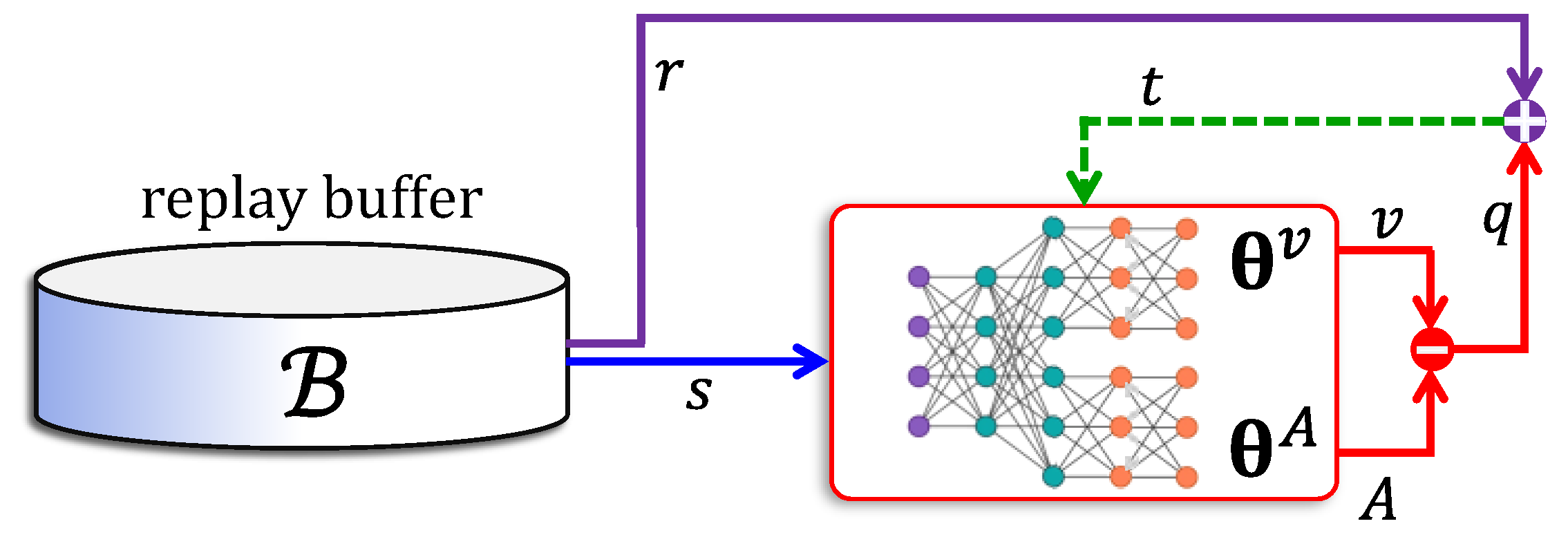
Actor–critic methods combine policy gradient and value-based RL methods [93]. The actor–critic architecture consists of two learning agents, the actor and the critic (see Figure 11). From any environmental state, the actor is trained using policy gradient to respond with an action. The critic is trained with a value-based RL method to evaluate the effectiveness of the actor’s output, which is then used to train the latter.

Let us denote the actor’s and the critic’s parameters with the symbols ${\mathsf{\theta }}^a$ and ${\mathsf{\theta }}^c$. The critic network can be modeled as a DQN, although it is trained with the advantage function as defined in Equation (13). When the environmental state is$s_t\left(n\right)$, for every action $a_t\left(n\right)$ the critic network provides as its output, the value of the state–action pair $q\left(s_t\left(n\right),a_t\left(n\right)|{\mathsf{\theta }}^c\right)$. The actor is incremented using gradient ascent,

$$\begin{array}{c}{\mathsf{\theta }}^a\leftarrow {\mathsf{\theta }}^a+{\eta }^a\frac{1}{T}{\displaystyle {\displaystyle \sum }_t}q\left(s_t\left(n\right),a_t\left(n\right)|{\mathsf{\theta }}^c\right){\nabla }_{{\mathsf{\theta }}^a}\log {\pi }_{{\mathsf{\theta }}^a}\left(a_t\left(n\right)|s_t\left(n\right);{\mathsf{\theta }}^a\right)\end{array}$$

(38)

Equation (38) shown above closely resembles the policy gradient increment in Equation (30) (with $b=0$). The only difference is that the critic is used in order to compute the gradient’s weight $q\left(s_t\left(n\right),a_t\left(n\right)|{\mathsf{\theta }}^c\right)$.

The update rule for the critic network, which is similar to Equation (22), is shown below,

$$\begin{array}{c}{\mathsf{\theta }}^c\leftarrow {\mathsf{\theta }}^c-{\eta }^c\frac{1}{T}{\displaystyle {\displaystyle \sum }_t}\left(q\left(s_t,a_t|{\mathsf{\theta }}^c\right)-(r_t+q\left(s_{t+1},a_{t+1}|{\mathsf{\theta }}^c\right)\right){\nabla }_{{\mathsf{\theta }}^c}q\left(s_t,a_t|{\mathsf{\theta }}^c\right)\end{array}$$

(39)

The advantage actor–critic (A2C) algorithm [94] is very effective in reducing the variance in the policy gradient algorithm of the actor. The A2C architecture entails a two-fold improvement over the ‘vanilla’ actor–critic method, which are outlined below.

(i)

The actor network uses an advantage function $A\left(s_t,a_t\right)$, which is the difference between a return value $R$ and the value of state $v\left(s_t|{\mathsf{\theta }}^c\right)$. Accordingly, the critic is trained to approximate the value function.

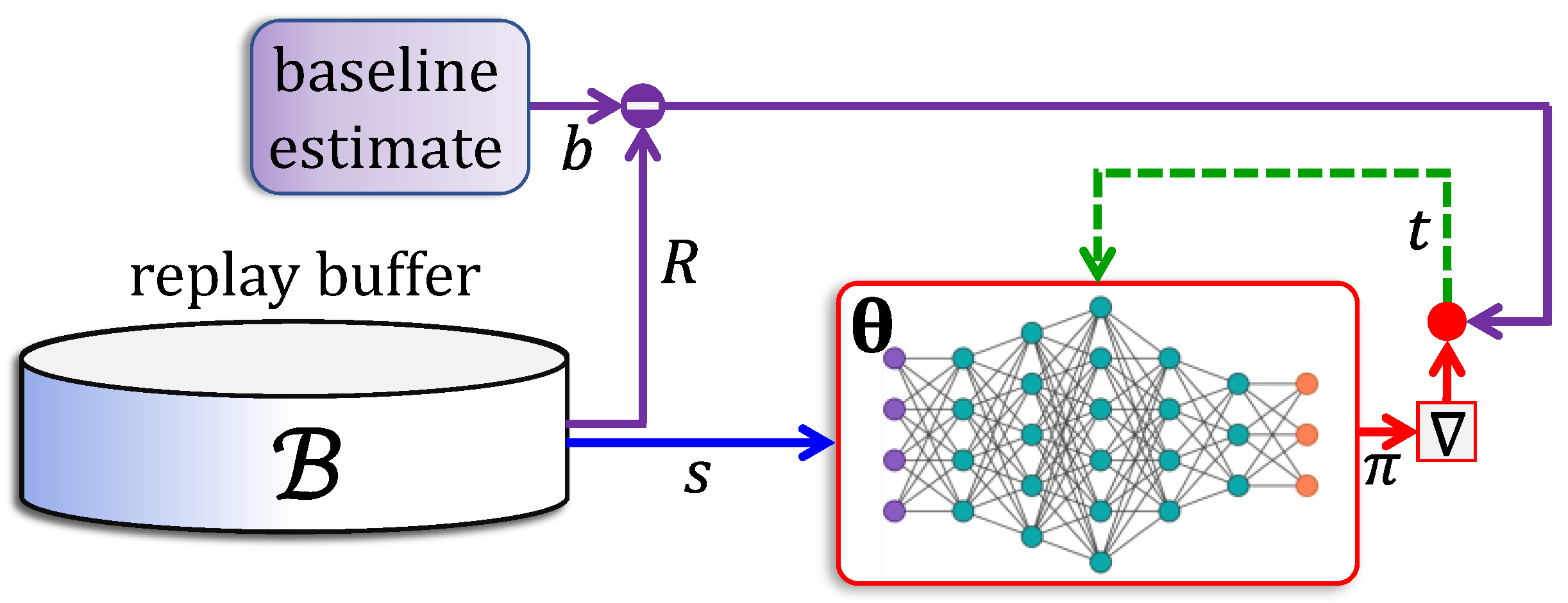
(ii)

The reward $R$ is computed using a $\tau$-step lookahead feature, where the log-gradient is weighted using the sum of the next $\tau$ rewards.

To better understand how the $\tau$-step lookahead works, let us turn our attention to Equation (30). In this expression the gradient ${\nabla }_{\mathsf{\theta }}\log {\pi }_{\mathsf{\theta }}\left(a_t|s_t\right)$ at time instant $t$ is weighted by the factor $\left(R\left(\mathcal{E}\right)-b\right)$ where $R\left(\mathcal{E}\right)$ is the return of an entire episode from $t=0$ until $T-1$, so that $R\left(\mathcal{E}\right)=r_0+\gamma r_1+\dots {\gamma }^t{r}_t+\dots {\gamma }^{t+\tau }{r}_{t+\tau }+\dots {\gamma }^{T-1}{r}_{T-1}.$ The baseline is $b$ is the value of $v\left(s_t|{\mathsf{\theta }}^C\right)$. It is reasoned that the sum of the past rewards $r_0+\gamma r_1+\dots {\gamma }^{t-1}{r}_{t-1}$ does not have any bearing on the quality of the action $a_t$ taken at the instant $t$. Hence all past rewards are dropped from $R$. Furthermore, rewards received in the distant future, i.e., after $\tau$ instants are also dropped. In other words, $R$ consists of the sum of the discounted rewards between the instant $t$ and the instant $t+\tau$. Whereupon, the actor’s update rule is expressed as,

$$\begin{array}{c}{\mathsf{\theta }}^a\leftarrow {\mathsf{\theta }}^a+{\eta }^a\frac{1}{T}{\displaystyle {\displaystyle \sum }_{t=0}^{T-\tau }}{\nabla }_{{\mathsf{\theta }}^a}\log {\pi }_{{\mathsf{\theta }}^a}\left(a_t|s_t\right)\left({\displaystyle {\displaystyle \sum }_{t^{\prime }=0}^{\tau }}{r}_{t+t^{\prime }}-v\left(s_t|{\mathsf{\theta }}^c\right)\right)\end{array}$$

(40)

The critic is updated using the same return $R$, in accordance with the expression shown below,

$$\begin{array}{c}{\mathsf{\theta }}^c\leftarrow {\mathsf{\theta }}^c-{\eta }^c\frac{1}{T\left|\mathcal{B}\right|}{\displaystyle {\displaystyle \sum }_{t=0}^{T-\tau }}\left(v\left(s_t|{\mathsf{\theta }}^c\right)-{\displaystyle {\displaystyle \sum }_{t^{\prime }=0}^{\tau }}{r}_{t+t^{\prime }}\right){\nabla }_{{\mathsf{\theta }}^c}v\left(s_t|{\mathsf{\theta }}^c\right)\end{array}$$

(41)

The asynchronous advantage actor–critic (A3C) method [94] is an extension of A2C that can be applied in parallel processing environments. A global network and a set of ‘workers’ are maintained in A3C. Each worker receives the actor and critic parameters that it implements on its own independent environment and collecting reward signals. The rewards are then used to determine increments $\mathrm{\Delta }{\mathsf{\theta }}^A$ and $\mathrm{\Delta }{\mathsf{\theta }}^C$, which are then used to asynchronously update the parameters in the global network. An advantage of A3C is that due to the parallel action of multiple workers, an experience replay buffer does not have to be incorporated.

The deterministic policy gradient (DPG) algorithm was described in [85], and more recently in SLH+14]. It was later extended to a deep framework in [95], known as the deep deterministic policy gradient (DDPG). DDPG is an off-policy actor–critic method that concurrently learns the optimal Q-function $q^{\ast }$, as well as the optimal policy ${\pi }^{\ast }$.

In any off-policy actor–critic model, the critic must be trained to output the optimal policy ${\pi }^{\ast }$. Hence, the term $q\left(s_{t+1},a_{t+1}\right)$ in Equation (39) should be replaced with the maximum over all actions $q\left(s_{t+1},a^{\ast }\right)$, where the optimal action $a^{\ast }=\underset{a\in \mathbb{A}}{\mathrm{argmax}} q\left(s_{t+1},a\right)$ as in Equation (19). Unfortunately, when the action space $\mathbb{A}$ is continuous ($\left|\mathbb{A}\right|=\infty$) an exhaustive search to find $a^{\ast }$ is impossible. Moreover, in a majority of applications, using numerical optimization to obtain $a^{\ast }$ is computationally too intensive to be used within the training algorithm.

In order to circumvent these difficulties in identifying the optimal action that maximizes the Q-value, there are three options available for use. These are outlined below.

(i)

$q\left(s_{t+1},a\right)$ can be sampled for several different actions and $a^{\ast }$ be assigned the action corresponding to the sample maximum [96].

(ii)

A convex approximation of $q\left(s,a\right)$ around $s_{t+1}$ can be devised and $a^{\ast }$ obtained over the approximate function [97].

(iii)

A separate off-policy policy network can be used to learn the optimal policy ${\pi }^{\ast }$ [98].

Out of the above three available options discussed above, the third and last has been adopted in DDPG. The critic parameter ${\mathsf{\theta }}^c$ is updated in accordance with the expression shown below,

$$\begin{array}{c}{\mathsf{\theta }}^c\leftarrow {\mathsf{\theta }}^c-{\eta }^c\frac{1}{T\left|\mathcal{B}\right|}{\displaystyle {\displaystyle \sum }_{n\in \mathcal{B}, t}}\left(r_t+q\left(s_{t+1}\left(n\right),a_{t+1}\left(n\right)|{\mathsf{\theta }}^c\right)-q\left(s_t\left(n\right),\pi \left(s_t\left(n\right)|{\mathsf{\theta }}^a\right)\right)\right){\nabla }_{{\mathsf{\theta }}^c}q\left(s_t\left(n\right),a_t\left(n\right)|{\mathsf{\theta }}^c\right)\end{array}$$

(42)

In Equation (42), $\pi \left(s_t\left(n\right)|{\mathsf{\theta }}^a\right)$ is the output of DDPG’s actor. DDPG uses a replay buffer $\mathcal{B}$ that includes samples from older policies. The actor’s parameter ${\mathsf{\theta }}^a$ is trained using any off-policy policy gradient as in Equation (37).

One of the drawbacks of DDPG is the problem of overestimation [99]. Suppose during the course of training, the function $q\left(s,a|{\mathsf{\theta }}^c\right)$ acquires a sharp local peak. Under these circumstances, further training would converge towards this local optimum, leading to undesirable results. This issue has been tackled by twin delayed deterministic policy gradient (TD3) in [80]. TD3 maintains a pair of critics whose parameters we shall denote as ${\mathsf{\theta }}^{c_1}$ and ${\mathsf{\theta }}^{c_2}$, or more concisely as ${\mathsf{\theta }}^{c_i}$, where $i\in \left\{1,2\right\}$.

In Equation (42), it can be seen that DDPG has a target $r_t+q\left(s_{t+1}\left(n\right),a_{t+1}\left(n\right)|{\mathsf{\theta }}^c\right)$ where $q\left(s_{t+1}\left(n\right),a_{t+1}\left(n\right)|{\mathsf{\theta }}^c\right)$ is obtained from the critic. TD3 has two targets, $q\left(s_{t+1}\left(n\right),a_{t+1}\left(n\right)|{\mathsf{\theta }}^{c_i}\right)$, $i\in \left\{1,2\right\}$. The actions $a_{t+1}\left(n\right)$ in TD3 are clipped to lie within the interval $\left[a_{\min },a_{ \max }\right]$. In order to increase exploration, Gaussian noise is added to this action. Finally, the target is obtained as $r_t+\underset{i\in \left\{1,2\right\}. }{\min }q\left(s_{t+1}\left(n\right),a_{t+1}\left(n\right)|{\mathsf{\theta }}^{c_i}\right)$, which is used for training.

The soft actor–critic (SAC) RL proposed recently in [81,100] is an off-policy RL approach. The striking feature of SAC is the presence of an entropy term in the objective function,

$$\begin{array}{c}J\left(\mathsf{\theta }\right)={\mathbb{E}}_{{\pi }_{\mathsf{\theta }}}\left[r_t+\alpha H\left({\pi }_{\mathsf{\theta }}|s_t\right)\right]\end{array}$$

(43)

Incorporating the entropy $H\left({\pi }_{\mathsf{\theta }}|s_t\right)$ in Equation (43) increases the degree of randomness in the policy which helps in exploration. As with TD3, SAC uses two critic networks.

6. Use of Reinforcement Learning in Home Energy Management Systems

This section addresses aspects of the survey on the use of RL approaches for various HEMS applications. All articles in this survey have been published in established technical journals that were published or made available online within the past five years.

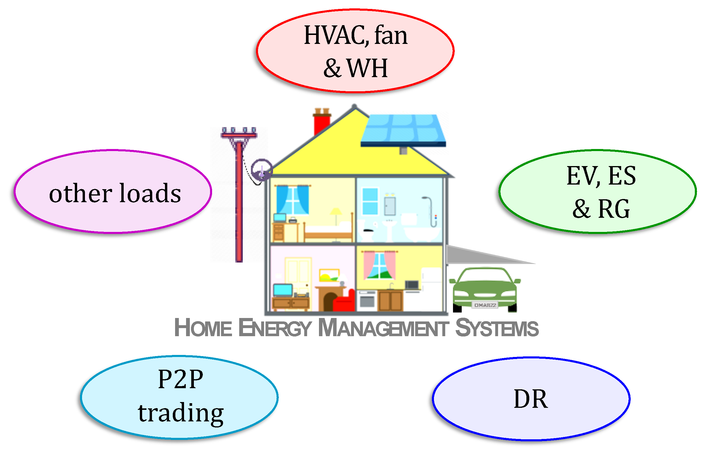
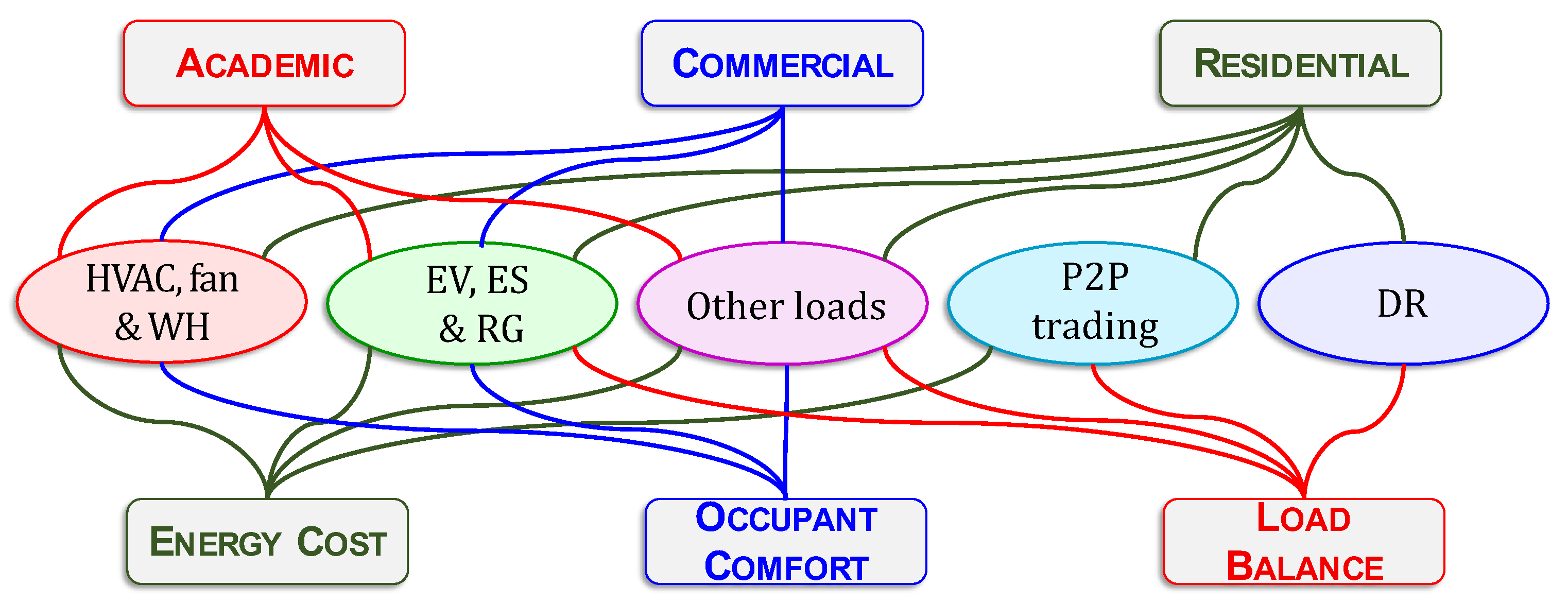
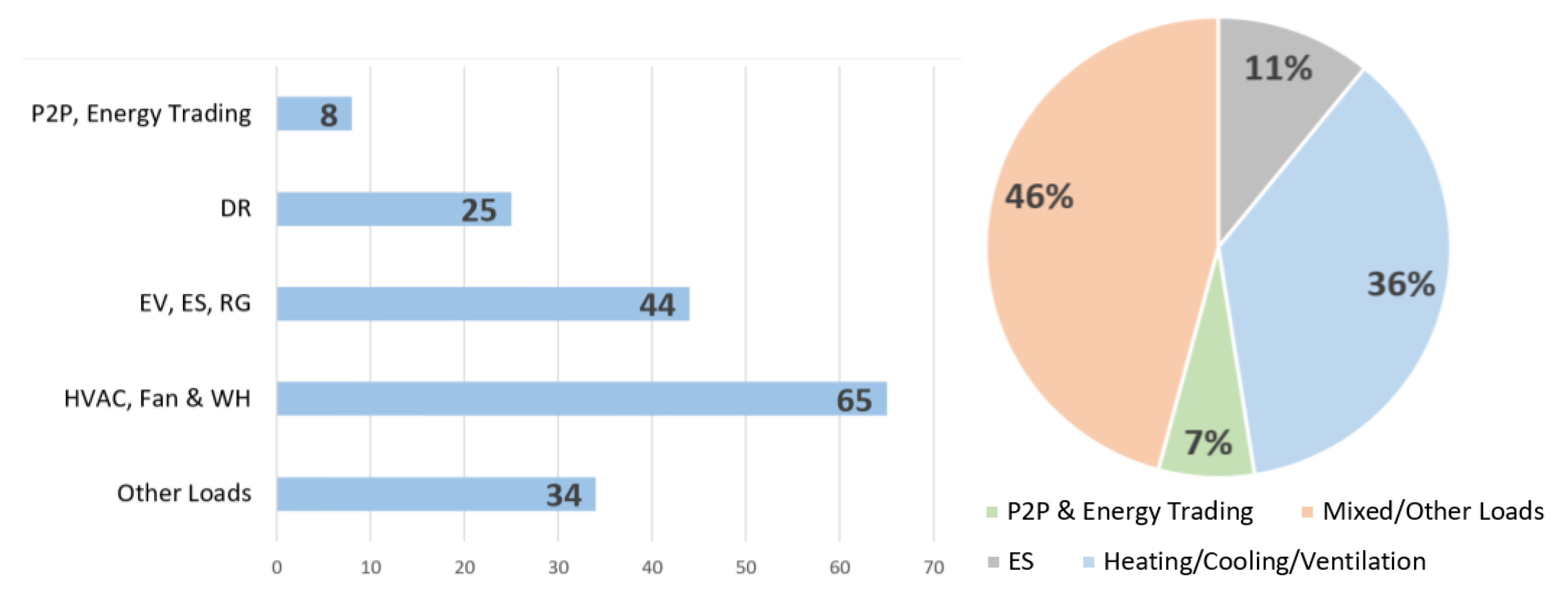
6.1. Application Classes

In this study, all applications were divided into five classes as in Figure 12 below.

(i)

Heating, Ventilation and Air Conditioning, Fans and Water Heaters: Heating, ventilation, and air conditioning (HVAC) systems alone are responsible for about half of the total electricity consumption [48,101,102,103,104]. In this survey, HVAC, fans and water heaters (WH) have been placed under a single category. Effective control of these loads is a major research topic in HEMS.

(ii)

Electric Vehicles, Energy Storage, and Renewable Generation: The charging of electric vehicles (EVs) and energy storage (ES) devices, i.e., batteries are studied in the literature as in [105,106]. Wherever applicable, EV and ES must be charged in coordination with renewable generation (RG) such as solar panels and wind turbines. The aim is to make decisions in order to save energy costs, while addressing comfort and other consumer requirements. Thus, EV, ES, and RG have been placed under a single class for the purpose of this survey.

(iii)

Other Loads: Suitable scheduling of several home appliances such as dishwasher, washing machine, etc., can be achieved through HEMS to save energy usage or cost. Lighting schedules are important in buildings with large occupancy. These loads have been lumped into a single class.

(iv)

Demand Response: With the rapid proliferation of green energies into homes and buildings, and these sources merged into the grid, demand response (DR) has acquired much research significance in HEMS. DR programs help in load balancing, by scheduling and/or controlling shiftable loads and in incentivizing participants [107,108] to do so through HEMS. RL for DR is one of the classes in this survey.

(v)

Peer-to-Peer Trading: Home energy management has been used to maximize the profit for the prosumers by trading the electricity with each other directly in peer-to-peer (P2P) trading or indirectly through a third party as in [109]. Currently, theoretical research on automated trading is receiving significant attention. P2P trading is the fifth and final application category to have been considered in this survey.

Each application class is associated with an objective function and a building type that are discussed in subsequent paragraphs. The schematic in Figure 13 shows all links that have been covered by the articles in this survey.

Figure 14 shows the number of research articles that applied RL to each class. Note that a significant proportion of these papers addressed more than one class. More than third of the papers we reviewed focused only on HVAC, fans and water heaters. Just above 10% of the papers studied RL control for the energy storage (ES) systems. Only 7% of the papers focused on the energy trading. However, most of the papers (46%) are targeting more than one object. These results are shown in Figure 14.

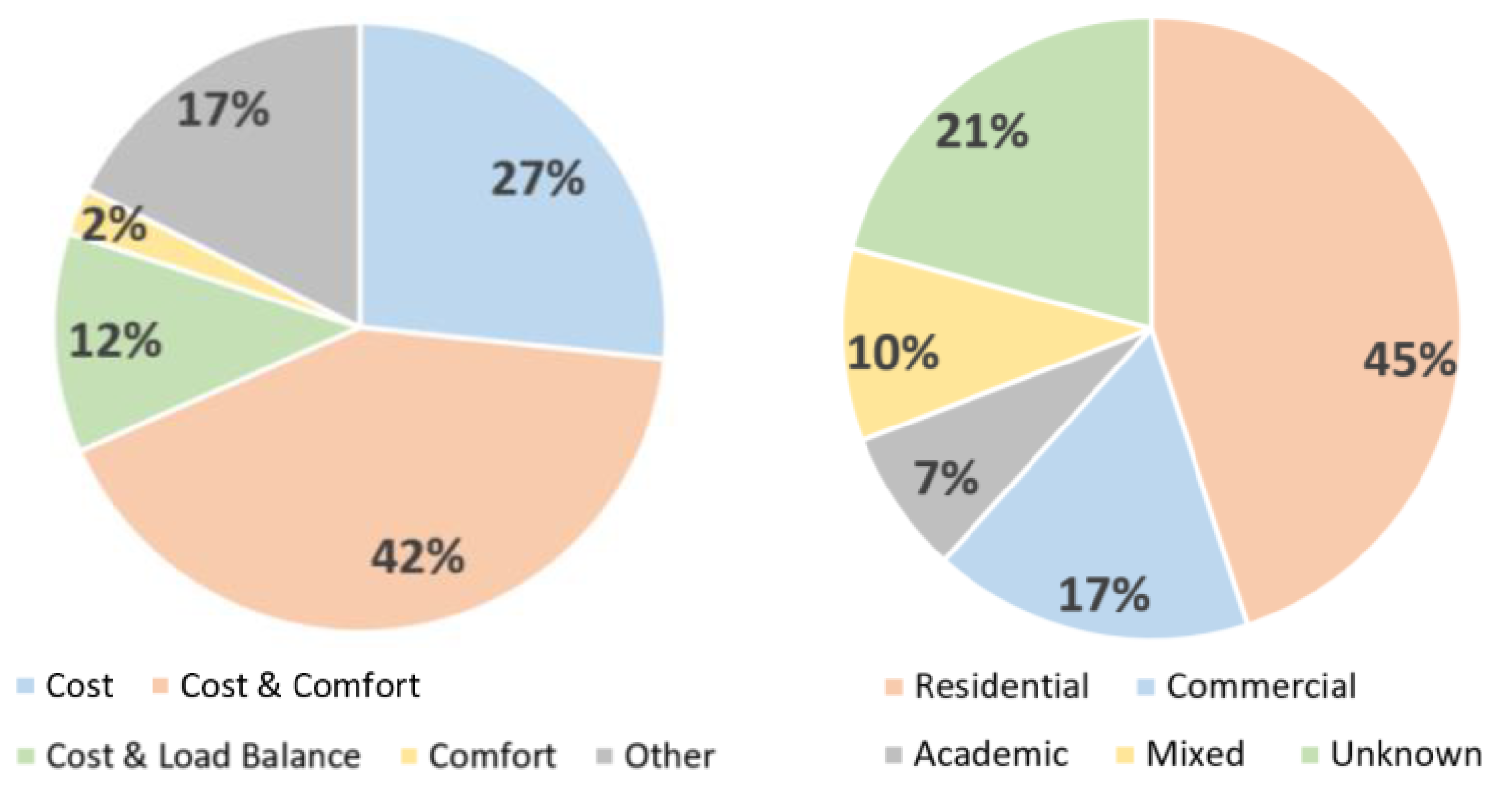
6.2. Objectives and Building Types

Within these HEMS applications, RL has been applied in several ways. It has been used to reduce energy consumption within residential units and buildings [110]. It has also been used to achieve a higher comfort level for the occupants [111]. In operations at the interface between the residential units and the energy grid, RL has been applied to maximize prosumers profit in energy trading as well as for load balancing.

For this purpose, we break down the objectives into three different types as listed below.

(i)

Energy Cost: The cost of using any electrical device by the consumer and in most of the cases it is proportionally related to its energy consumption. In this paper we use the terms ‘cost’ and ‘consumption’ interchangeably.

(ii)

Occupant Comfort: the main factor that can affect the occupant’s comfort is the thermal comfort, which depends mainly on the room temperature and humidity.

(iii)

Load Balance: Power supply companies try to achieve load balance by reducing the power consumption of consumers at peak periods to match the station power supply. The consumers are motivated to participate in such programs by price incentives.

Figure 13 illustrates the RL objectives that were used in each application class.

Next, all buildings and complexes were categorized into the following three types.

(i)

Residential: for the purpose of this survey, individual homes, residential communities, as well as apartment complexes fall under this type of building.

(ii)

Commercial: these buildings include offices, office complexes, shops, malls, hotels, as well as industrial buildings.

(iii)

Academic: academic buildings range from schools, university classrooms, buildings, research laboratories, up to entire campuses.

The research literature in this survey revealed that for residential buildings, RL was applied in all five application classes. However, in case of commercial and academic buildings, RL was typically applied to the first three categories, i.e., to HVAC, fans and WH, to EVs, ESs and RGs, as well as to other loads. This is shown in Figure 13.

Figure 15 illustrates the outcome of this survey. It may be noted that in the largest proportion of articles (42%) the RL algorithm took into account both cost and comfort. About 27% of all articles addressed cost as the only objective, thereby defining the second largest proportion.

6.3. Deployment, Multi-Agents, and Discretization

The proportion of research articles where RL was actually deployed in the real world was studied. It was found that only 12% of research articles report results where RL was used with real HEMS. The results are consistent with an earlier survey [49] where this proportion was 11%. The results are shown in Figure 16.

7. Reinforcement Learning Algorithms in Home Energy Management Systems

This section focuses on how the RL and DRL algorithms described in earlier sections were used in HEMS applications. The references have been categorized in terms of the application class, objective function, and building type, that were described in the immediately preceding section.

Table 1. References using Tabular Reinforcement Learning.

Reference	Application	Objective	Building Type	Algorithm
[112]	HVAC, Fans, WH	Cost	Residential	Q-Learning
[113]		Cost and Comfort
[114,115]		Other	Academic
[116]		Comfort	Mixed/NA
[117]		Other
[109,118]	P2P Trading	Cost
[119,120]			Residential
[121]	EV, ES, and RG
[122,123]			Mixed/NA
[124]		Other	Residential
[125,126]	Other/Mixed	Cost and Comfort	Commercial
[127]			Academic
[107,128,129,130,131,132]			Residential
[133]		Other
[134,135]		Cost
[136]			Mixed/NA
[137]		Cost and Comfort
[138,139]		Cost and Load Balance
[140]		Other
[141]	P2P Trading	Cost		Distributed RL
[142,143,144]	HVAC, Fans, WH	Cost and Comfort	Residential	Other (FQI)
[145]		Comfort	Commercial	Q-Learn. and SARSA
[146]		Cost and Comfort	Residential	SARSA
[147]	Other/Mixed	Cost and Load Balance		Policy Learning
[148]		Other
[149]		Cost and Comfort	Commercial	Model Based RL
[150]	HVAC, Fans, WH	Cost	Residential	Other (CARLA)
[151]		Cost and Comfort	Commercial	Other (Context. RL)

provides a list of references that used tabular RL methods. About 28% of articles used tabular methods.

In a similar manner,

Table 2. References using Deep Q Networks.

Reference	Application	Objective	Building Type	Algorithm
[152,153]	Other/Mixed	Cost	Residential	DQN
[154]		Cost and Load Balance
[105]	EV, ES, and RG	Cost
[155]		Other
[156]		Cost and Comfort
[157]	HVAC, Fans, WH	Cost
[158]	Other/Mixed		Commercial
[159]		Cost and Comfort
[160,161]	HVAC, Fans, WH		Mixed/NA
[162,163]	Other/Mixed	Cost
[164,165,166]	HVAC, Fans, WH	Cost and Comfort	Residential	DDQN
[167]			Academic
[168]		Comfort	Commercial
[169]	Other/Mixed	Cost and Load Balance	Residential
[106]		Cost and Comfort		Dueling-DQN
[170]	HVAC, Fans, WH	Cost		Other (FQI-LSTM, FQI-CNN)

considers references that used DQN. Most algorithms in the survey used DQN. However, DDQN was also popular in the HEMS research community. The survey found that dueling-DQN was applied in only one article.

Table 3. References using Deep Policy Networks.

Reference	Application	Objective	Building Type	Algorithm
[171]	HVAC, Fans, WH	Cost and Comfort	Academic	PPO
[172]			Commercial
[173]	P2P Trading	Other	Mixed/NA
[174]	EV, ES, and RG
[175]	Other/Mixed	Cost
[176]		Cost and Comfort	Residential	TRPO

categorizes references in the survey that used deep policy learning. PPO and TRPO are the only approaches that have been used so far in HEMS.

The survey also indicates that actor–critic was the preferred approach in comparison with deep policy learning.

Table 4. References using Actor–Critic Networks.

Reference	Application	Objective	Building Type	Algorithm
[177,178]	HVAC, Fans, WH	Cost and Comfort	Residential	DDPG
[61,179,180,181]	Other/Mixed
[182,183]		Cost and Load Balance
[184]		Cost
[185]	EV, ES, and RG
[186]	Other/Mixed	Cost and Comfort	Academic
[187]		Other
[188,189]	EV, ES, and RG		Commercial
[190,191,192]	HVAC, Fans, WH	Cost and Comfort	Mixed/NA
[193,194,195]	EV, ES, and RG	Other
[196,197]	Other/Mixed	Cost and Load Balance	Residential	SAC
[198,199]	HVAC, Fans, WH	Cost	Commercial
[103,200,201,202]		Cost and Comfort
[203]	Other/Mixed
[204]			Academic
[205,206,207]	HVAC, Fans, WH	Cost and Load Balance	Mixed/NA
[208,209,210]		Cost and Comfort
[211]	Other/Mixed		Residential	A2C
[212]	HVAC, Fans, WH	Cost	Commercial	A3C
[213]	P2P Trading		Mixed/NA	TD3
[214]	HVAC, Fans, WH
[215]		Cost and Comfort
[216]	Other/Mixed		Residential

provides a list of references that applied actor–critic learning, which constituted 53% of all deep learning methods. It shows that PPO is more popular than TRPO. We believe that this observation is due to the closer recency of the latter algorithm. References that used either a combination of two or more approaches, or any other approach not commonly used in RL literature, are shown in

Table 5. References using Combination of Methods and/or Miscellaneous Methods.

Reference	Application	Objective	Building Type	Algorithm
[60]	Other/Mixed	Cost and Comfort	Residential	DQN, DDPG
[217]				DQN, DDQN
[218]		Cost and Load Balance		DQN, DPG
[219]	P2P Trading			Other (Model-Based DRL)
[220]	HVAC, Fans, WH	Cost and Comfort	Academic	SAC, TD3, TRPO, PPO
[221]			Mixed/NA	Other (Clustering DRL)
[222]	EV, ES, and RG			PPO, TD3
[223]		Cost and Load Balance	Commercial	DDPG, DDQN, DQN

.

8. Conclusions

This article surveys how effectively RL has been leveraged for various HEMS applications. The survey reveals the following:

(i)

Although 66% of all articles used deep RL, many articles used tabular learning. This may indicate that only simplified application were considered.

(ii)

Around 53% of all articles used discrete states and actions. This is another indication that the HEMS scenarios may have been simplified.

(iii)

Around 12% of all approaches covered in this survey were deployed in the real world, their use being limited to simulation platforms only.

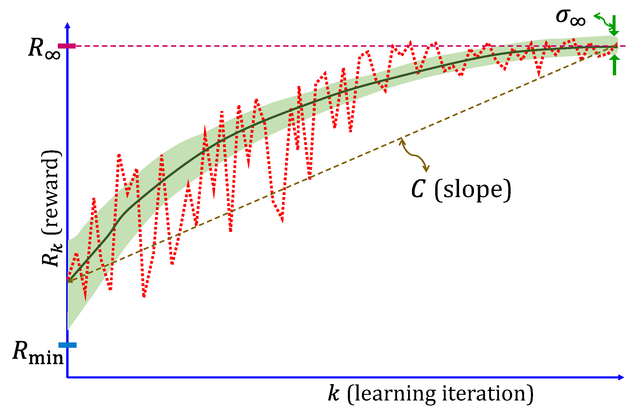
These observations strongly suggest that the use of RL in HEMS application is at a research stage and is yet to gain maturity. More in-depth investigation is necessary, particularly on RL algorithms that use DNN agents. Nonetheless, it was seen that 36% of all articles made use of multiagent schemes, which is an encouraging sign.

The only truly viable alternative is to use nonlinear control, more specifically model predictive control (MPC) [224]. MPC is widely used in various engineering applications (cf. [225]). The benefit of MPC is in the explicit manner by which it handles physical constraints. At each iteration, MPC considers a receding time horizon into the future, and applies a constrained optimization algorithm to determine the best control actions. However, in most cases, MPC uses linear or quadratic objective functions. This is a basic limitation that must be taken into account before applying MPC to large-scale problems and is in sharp contrast to RL that does not place any restriction on the reward signal. Moreover, MPC is a model-based approach, whereas an overwhelming majority of references in this survey used model-free RL methods ([149] being the sole exception).

There is a diverse array of algorithms available in the RL literature. Since tabular methods require discrete states and actions, and furthermore, that these spaces have low cardinalities, they may not be much use for most HEMS applications. Not surprisingly, this survey shows that tabular methods have been used less frequently than DNN methods. In future, as the HEMS community investigates increasingly complex HEMS domains, tabular methods would become even less likely to be used. Consequently, the choice of algorithm would usually be confined to DNN methods.

Out of the DNN methods, it must be noted that DQN and its derivatives can only be used in applications only when the action space is finite and small, such as in controlling OFF–ON switches. The survey reveals that actor–critic methods, which include Q-learning and policy learning, are the most popular in HEMS applications. Another deciding factor is whether to use policy-free or policy-based RL. On-policy learning may be used is applications where abandoning the policy in the initial stages may occasionally very negatively impact the environment. Thus, they may be used if the environment does not require too much exploration. On the other hand, off-policy RL can discover more novel policies.

Unlike in the unsupervised and supervised learning where simple performance metrics are readily available, performance evaluation in RL is an open problem [226]. The steadily increasing reward with iteration is the best means for any real application. The authors suggest that the following four criteria should be considered.

(i)

Saturation reward ($R_{\infty }$): the expected reward must be relatively high at saturation.

(ii)

Variance at saturation (${\sigma }_{\infty }$): the reward must not have excessive variance at saturation.

(iii)

Exploitation risk ($R_{\min }$): The minimum possible reward must not be so low that the environment is adversely affected. This is the risk associated with exploration and tends to occur during the initial exploratory stages of the RL training.

(iv)

Convergence rate ($C$): the number of iterations before the reward starts to saturate should not be large.

Figure 17 shows how to graphically interpret $R_{\infty }$, ${\sigma }_{\infty }$, $R_{\min }$, $C$.

Since the articles in this survey have always used some HEMS simulation platform, it is assumed that the RL algorithm can be run at least a few times. The above four performance metrics ($R_{\infty }$, ${\sigma }_{\infty }$, $R_{\min }$, $C$) proposed by the authors can be empirically estimated using Monte Carlo samples of such runs. Suppose the sequence of rewards obtained from the $i$^th run is $\left\{R_0^i, R_1^i, \dots , R_k^i, \dots , R_{K_i^{ \max }}^i\right\}$. Each $R_k^i$ is some reward and $k$ represents an iteration of the RL algorithm. The precise meanings of the terms (reward and iteration) are entirely dependent on the specific HEMS application, how the reward function is implemented, whether a replay buffer is used, and the RL algorithm.

A reward $R_k^i$ may be the either an aggregate return value, the instantaneous reward at the time horizon $T$, or the reward at last parameter update, etc. Likewise, the iteration index $k$ may be an instantaneous time step $t \left(t\le T\right)$, Alternately, $k$ may refer to the number of times the training algorithm adjusts the model parameter $\mathsf{\theta }$, or flushes the replay buffer, etc. The exact meanings of the terms are left to the reader. However it must be remembered that at the beginning of each run, all relevant model parameters should be reinitialized, that at the end of each run after $K_i^{ \max }$ iterations (subscripted since $K_i^{ \max }$ may vary with run), the RL training algorithm converges to a different final model parameter, and that $R_{K_i^{ \max }}^i$ truly reflects the quality of the model. Moreover, it must be ensured that the algorithm terminates after $R_k^i$ attains saturation—i.e., there is no perceptible gain from more iterations.

If the runs are indexed $i=1,2,\dots ,\left|\mathcal{I}\right|$ where $\mathcal{I}$ is the set of runs, the suggested performance metrics can be estimated as,

$$\begin{array}{c}{R}_{\infty }\approx \frac{1}{\left|\mathcal{I}\right|}{\displaystyle {\displaystyle \sum }_{i\in \mathcal{I}}}{R}_{K_i^{ \max }}^i\end{array}$$

(44)

$$\begin{array}{c}{\sigma }_{\infty }\approx \frac{1}{\left|\mathcal{I}\right|-1}{\displaystyle {\displaystyle \sum }_{i\in \mathcal{I}}}{\left(R_{K_i^{ \max }}^i-{\widehat{R}}_{\infty }\right)}^2\end{array}$$

(45)

$$\begin{array}{c}{R}_{\min }\approx \underset{i\in \mathcal{I}}{\min }\underset{k}{ \min }{R}_k^i \left(\mathrm{or}, R_{\min }\approx \underset{i\in \mathcal{I}}{\min }{R}_1^i\right)\end{array}$$

(46)

$$\begin{array}{c}C\approx \frac{1}{\left|\mathcal{I}\right|}{\displaystyle {\displaystyle \sum }_{i\in \mathcal{I}}}\frac{R_0^i-R_{K_i^{ \max }}^i}{K_i^{ \max }}\end{array}$$

(47)

In Equation (46), it is assumed that ${\widehat{R}}_{\infty }$ is the estimated average value of $R_{\infty }$, determined in accordance with Equation (45). In some situations, it may be computationally too expensive to obtain multiple runs. In such cases, as well as when the RL is implemented on a real HEMS environment, $\mathcal{I}$ may be a singleton set ($\left|\mathcal{I}\right|=1$). In this case, ${\sigma }_{\infty }$ in Equation (46) is meaningless. An alternate metric may be used by using the last few iterations before termination.

References

1. U.S. Energy Information Administration. Electricity Explained: Use of Electricity. 14 May 2021. Available online: www.eia.gov/energyexplained/electricity/use-of-electricity.php (accessed on 10 April 2022).
2. Center for Sustainable Systems. U.S. Energy System Factsheet. Pub. No. CSS03-11; Center for Sustainable Systems, University of Michigan: Ann Arbor, MI, USA, 2021; Available online: https://css.umich.edu/publications/factsheets/energy/us-energy-system-factsheet (accessed on 10 April 2022).
3. Shakeri, M.; Shayestegan, M.; Abunima, H.; Reza, S.S.; Akhtaruzzaman, M.; Alamoud, A.; Sopian, K.; Amin, N. An intelligent system architecture in home energy management systems (HEMS) for efficient demand response in smart grid. Energy Build. 2017, 138, 154–164. [Google Scholar] [CrossRef]
4. Leitão, J.; Gil, P.; Ribeiro, B.; Cardoso, A. A survey on home energy management. IEEE Access 2020, 8, 5699–5722. [Google Scholar] [CrossRef]
5. Shareef, H.; Ahmed, M.S.; Mohamed, A.; Al Hassan, E. Review on Home Energy Management System Considering Demand Responses, Smart Technologies, and Intelligent Controllers. IEEE Access 2018, 6, 24498–24509. [Google Scholar] [CrossRef]
6. Mahapatra, B.; Nayyar, A. Home energy management system (HEMS): Concept, architecture, infrastructure, challenges and energy management schemes. Energy Syst. 2019, 13, 643–669. [Google Scholar] [CrossRef]
7. Dileep, G. A survey on smart grid technologies and applications. Renew. Energy 2020, 146, 2589–2625. [Google Scholar] [CrossRef]
8. Zafar, U.; Bayhan, S.; Sanfilippo, A. Home energy management system concepts, configurations, and technologies for the smart grid. IEEE Access 2020, 8, 119271–119286. [Google Scholar] [CrossRef]
9. Alanne, K.; Sierla, S. An overview of machine learning applications for smart buildings. Sustain. Cities Soc. 2022, 76, 103445. [Google Scholar] [CrossRef]
10. Aguilar, J.; Garces-Jimenez, A.; R-Moreno, M.D.; García, R. A systematic literature review on the use of artificial intelligence in energy self-management in smart buildings. Renew. Sustain. Energy Rev. 2021, 151, 111530. [Google Scholar] [CrossRef]
11. Himeur, Y.; Ghanem, K.; Alsalemi, A.; Bensaali, F.; Amira, A. Artificial intelligence based anomaly detection of energy consumption in buildings: A review, current trends and new perspectives. Appl. Energy 2021, 287, 116601. [Google Scholar] [CrossRef]
12. Barto, A.G.; Sutton, R.S.; Anderson, C.W. Neuronlike elements that can solve difficult learning control problems. IEEE Trans. Syst. Man Cybern. 1983, 13, 835–846. [Google Scholar] [CrossRef]
13. Tesauro, G. TD-Gammon, a self-teaching backgammon program, achieves master-level play. Neural Comput. 1994, 6, 215–219. [Google Scholar] [CrossRef]
14. Peters, J.; Schaal, S. Reinforcement learning of motor skills with policy gradients. Neural Netw. 2008, 21, 682–697. [Google Scholar] [CrossRef]
15. Mnih, V.; Kavukcuoglu, K.; Silver, D.; Rusu, A.A.; Veness, J.; Bellemare, M.G.; Graves, A.; Riedmiller, M.; Fidjeland, A.K.; Ostrovski, G.; et al. Human-level control through deep reinforcement learning. Nature 2015, 518, 529–533. [Google Scholar] [CrossRef]
16. Silver, D.; Huang, A.; Maddison, C.J.; Guez, A.; Sifre, L.; van den Driessche, G.; Schrittwieser, J.; Antonoglou, I.; Panneershelvam, V.; Lanctot, M.; et al. Mastering the game of Go with deep neural networks and tree search. Nature 2016, 529, 484–489. [Google Scholar] [CrossRef]
17. Silver, D.; Schrittwieser, J.; Simonyan, K.; Antonoglou, I.; Huang, A.; Guez, A.; Hubert, T.; Baker, L.; Lai, M.; Bolton, A.; et al. Mastering the game of Go without human knowledge. Nature 2017, 550, 354–359. [Google Scholar] [CrossRef]
18. Arulkumaran, K.; Deisenroth, M.P.; Brundage, M.; Bharath, A.A. A brief survey of deep reinforcement learning. IEEE Signal Process. Mag. 2017, 34, 26–38. [Google Scholar] [CrossRef]
19. François-Lavet, V.; Henderson, P.; Islam, R.; Bellemare, M.G.; Pineau, J. An introduction to deep reinforcement learning. Found. Trends Mach. Learn. 2018, 11, 219–354. [Google Scholar] [CrossRef]
20. Silver, D.; Singh, S.; Precup, D.; Sutton, R.S. Reward is enough. Artif. Intell. 2021, 299, 103535. [Google Scholar] [CrossRef]
21. Goertzel, B. Artificial General Intelligence; Pennachin, C., Ed.; Springer: New York, NY, USA, 2007; Volume 2. [Google Scholar]
22. Zhang, T.; Mo, H. Reinforcement learning for robot research: A comprehensive review and open issues. Int. J. Adv. Robot. Syst. 2021, 18, 17298814211007305. [Google Scholar] [CrossRef]
23. Bhagat, S.; Banerjee, H.; Tse, Z.T.H.; Ren, H. Deep reinforcement learning for soft, flexible robots: Brief review with impending challenges. Robotics 2019, 8, 4. [Google Scholar] [CrossRef] [Green Version]
24. Lee, C.; An, D. AI-Based Posture Control Algorithm for a 7-DOF Robot Manipulator. Machines 2022, 10, 651. [Google Scholar] [CrossRef]
25. Shakhatreh, H.; Sawalmeh, A.H.; Al-Fuqaha, A.; Dou, Z.; Almaita, E.; Khalil, I.; Othman, N.S.; Khreishah, A.; Guizani, M. Unmanned Aerial Vehicles (UAVs): A survey on civil applications and key research challenges. IEEE Access 2019, 7, 48572–48634. [Google Scholar] [CrossRef]
26. Zeng, F.; Wang, C.; Ge, S.S. A survey on visual navigation for artificial agents with deep reinforcement learning. IEEE Access 2020, 8, 135426–135442. [Google Scholar] [CrossRef]
27. Sun, H.; Zhang, W.; Yu, R.; Zhang, Y. Motion planning for mobile robots-focusing on deep reinforcement learning: A systematic review. IEEE Access 2021, 9, 69061–69081. [Google Scholar] [CrossRef]
28. Luong, N.C.; Hoang, D.T.; Gong, S.; Niyato, D.; Wang, P.; Liang, Y.-C.; Kim, D.I. Applications of deep reinforcement learning in communications and networking: A survey. IEEE Commun. Surv. Tutor. 2019, 21, 3133–3174. [Google Scholar] [CrossRef]
29. Zhang, G.; Li, Y.; Niu, Y.; Zhou, Q. Anti-jamming path selection method in a wireless communication network based on Dyna-Q. Electronics 2022, 11, 2397. [Google Scholar] [CrossRef]
30. Zhang, Y.; Zhu, J.; Wang, H.; Shen, X.; Wang, B.; Dong, Y. Deep reinforcement learning-based adaptive modulation for underwater acoustic communication with outdated channel state information. Remote Sens. 2022, 14, 3947. [Google Scholar] [CrossRef]
31. Ullah, Z.; Al-Turjman, F.; Mostarda, L. Cognition in UAV-aided 5G and beyond communications: A survey. IEEE Trans. Cogn. Commun. Netw. 2020, 6, 872–891. [Google Scholar] [CrossRef]
32. Nguyen, T.T.; Reddi, V.J. Deep reinforcement learning for cyber security. arXiv 2019, arXiv:1906.05799. [Google Scholar] [CrossRef] [PubMed]
33. Alavizadeh, H.; Alavizadeh, H.; Jang-Jaccard, J. Deep Q-Learning Based Reinforcement Learning Approach for Network Intrusion Detection. Computers 2022, 11, 41. [Google Scholar] [CrossRef]
34. Jin, Z.; Zhang, S.; Hu, Y.; Zhang, Y.; Sun, C. Security state estimation for cyber-physical systems against DoS attacks via reinforcement learning and game theory. Actuators 2022, 11, 192. [Google Scholar] [CrossRef]
35. Zhu, H.; Cao, Y.; Wang, W.; Jiang, T.; Jin, S. Deep reinforcement learning for mobile edge caching: Review, new features, and open issues. IEEE Netw. 2018, 32, 50–57. [Google Scholar] [CrossRef]
36. Liu, Y.; Wu, F.; Lyu, C.; Li, S.; Ye, J.; Qu, X. Deep dispatching: A deep reinforcement learning approach for vehicle dispatching on online ride-hailing platform. Transp. Res. Part E Logist. Transp. Rev. 2022, 161, 102694. [Google Scholar] [CrossRef]
37. Liu, S.; See, K.C.; Ngiam, K.Y.; Celi, L.A.; Sun, X.; Feng, M. Reinforcement learning for clinical decision support in critical care: Comprehensive review. J. Med. Internet Res. 2020, 22, e18477. [Google Scholar] [CrossRef]
38. Elavarasan, D.; Vincent, P.M.D. Crop yield prediction using deep reinforcement learning model for sustainable agrarian applications. IEEE Access 2020, 8, 86886–86901. [Google Scholar] [CrossRef]
39. Garnier, P.; Viquerat, J.; Rabault, J.; Larcher, A.; Kuhnle, A.; Hachem, E. A review on deep reinforcement learning for fluid mechanics. Comput. Fluids 2021, 225, 104973. [Google Scholar] [CrossRef]
40. Cheng, L.-C.; Huang, Y.-H.; Hsieh, M.-H.; Wu, M.-E. A novel trading strategy framework based on reinforcement deep learning for financial market predictions. Mathematics 2021, 9, 3094. [Google Scholar] [CrossRef]
41. Kim, S.-H.; Park, D.-Y.; Lee, K.-H. Hybrid deep reinforcement learning for pairs trading. Appl. Sci. 2022, 12, 944. [Google Scholar] [CrossRef]
42. Zhu, T.; Zhu, W. Quantitative trading through random perturbation Q-network with nonlinear transaction costs. Stats 2022, 5, 546–560. [Google Scholar] [CrossRef]
43. Zhang, D.; Han, X.; Deng, C. Review on the research and practice of deep learning and reinforcement learning in smart grids. CSEE J. Power Energy Syst. 2018, 4, 362–370. [Google Scholar] [CrossRef]
44. Zhang, Z.; Zhang, D.; Qiu, R.C. Deep reinforcement learning for power system applications: An overview. CSEE J. Power Energy Syst. 2020, 6, 213–225. [Google Scholar] [CrossRef]
45. Jogunola, O.; Adebisi, B.; Ikpehai, A.; Popoola, S.I.; Gui, G.; Gacanin, H.; Ci, S. Consensus algorithms and deep reinforcement learning in energy market: A review. IEEE Internet Things J. 2021, 8, 4211–4227. [Google Scholar] [CrossRef]
46. Perera, A.T.D.; Kamalaruban, P. Applications of reinforcement learning in energy systems. Renew. Sustain. Energy Rev. 2021, 137, 110618. [Google Scholar] [CrossRef]
47. Chen, X.; Qu, G.; Tang, Y.; Low, S.; Li, N. Reinforcement learning for selective key applications in power systems: Recent advances and future challenges. IEEE Trans. Smart Grid 2022, 13, 2935–2958. [Google Scholar] [CrossRef]
48. Mason, K.; Grijalva, S. A review of reinforcement learning for autonomous building energy management. Comput. Electr. Eng. 2019, 78, 300–312. [Google Scholar] [CrossRef]
49. Wang, Z.; Hong, T. Reinforcement learning for building controls: The opportunities and challenges. Appl. Energy 2020, 269, 115036. [Google Scholar] [CrossRef]
50. Han, M.; May, R.; Zhang, X.; Wang, X.; Pan, S.; Yan, D.; Jin, Y.; Xu, L. A review of reinforcement learning methodologies for controlling occupant comfort in buildings. Sustain. Cities Soc. 2019, 51, 101748–101762. [Google Scholar] [CrossRef]
51. Yu, L.; Qin, S.; Zhang, M.; Shen, C.; Jiang, T.; Guan, X. A review of deep reinforcement learning for smart building energy management. IEEE Internet Things J. 2021, 8, 12046–12063. [Google Scholar] [CrossRef]
52. Zhang, H.; Seal, S.; Wu, D.; Bouffard, F.; Boulet, B. Building energy management with reinforcement learning and model predictive control: A survey. IEEE Access 2022, 10, 27853–27862. [Google Scholar] [CrossRef]
53. Vázquez-Canteli, J.R.; Nagy, Z. Reinforcement learning for demand response: A review of algorithms and modeling techniques. Appl. Energy 2019, 235, 1072–1089. [Google Scholar] [CrossRef]
54. Ali, H.O.; Ouassaid, M.; Maaroufi, M. Chapter 24: Optimal appliance management system with renewable energy integration for smart homes. Renew. Energy Syst. 2021, 533–552. [Google Scholar] [CrossRef]
55. Sharda, S.; Singh, M.; Sharma, K. Demand side management through load shifting in IoT based HEMS: Overview, challenges and opportunities. Sustain. Cities Soc. 2021, 65, 102517. [Google Scholar] [CrossRef]
56. Danbatta, S.J.; Varol, A. Comparison of Zigbee, Z-Wave, Wi-Fi, and Bluetooth wireless technologies used in home automation. In Proceedings of the 7th International Symposium on Digital Forensics and Security (ISDFS), Barcelos, Portugal, 10–12 June 2019; pp. 1–5. [Google Scholar] [CrossRef]
57. Withanage, C.; Ashok, R.; Yuen, C.; Otto, K. A comparison of the popular home automation technologies. In Proceedings of the 2014 IEEE Innovative Smart Grid Technologies - Asia (ISGT ASIA), Kuala Lumpur, Malaysia, 20–23 May 2014; 2014; pp. 600–605. [Google Scholar] [CrossRef]
58. Van de Kaa, G.; Stoccuto, S.; Calderón, C.V. A battle over smart standards: Compatibility, governance, and innovation in home energy management systems and smart meters in the Netherlands. Energy Res. Soc. Sci. 2021, 82, 102302. [Google Scholar] [CrossRef]
59. Rajasekhar, B.; Tushar, W.; Lork, C.; Zhou, Y.; Yuen, C.; Pindoriya, N.M.; Wood, K.L. A survey of computational intelligence techniques for air-conditioners energy management. IEEE Trans. Emerg. Top. Comput. Intell. 2020, 4, 555–570. [Google Scholar] [CrossRef]
60. Huang, C.; Zhang, H.; Wang, L.; Luo, X.; Song, Y. Mixed deep reinforcement learning considering discrete-continuous hybrid action space for smart home energy Management. J. Mod. Power Syst. Clean Energy 2022, 10, 743–754. [Google Scholar] [CrossRef]
61. Yu, L.; Xie, W.; Xie, D.; Zou, Y.; Zhang, D.; Sun, Z.; Zhang, L.; Zhang, Y.; Jiang, T. Deep reinforcement learning for smart home energy management. IEEE Internet Things J. 2020, 7, 2751–2762. [Google Scholar] [CrossRef]
62. Das, S. Deep Neural Networks. YouTube, 31 January 2022 [Video File]. Available online: www.youtube.com/playlist?list=PL_4Jjqx0pZY-SIO8jElzW0lNpzjcunOx4 (accessed on 1 April 2022).
63. Goodfellow, I.; Bengio, Y.; Courville, A. Deep Learning; MIT Press: Cambridge, MA, USA, 2016; Available online: https://www.deeplearningbook.org/ (accessed on 1 August 2022).
64. Achiam, J. Open AI, Part 2: Kinds of RL Algorithms. 2018. Available online: spinningup.openai.com/en/latest/spinningup/rl_intro2.html (accessed on 1 August 2022).
65. Bellman, R. Dynamic Programming; Rand Corporation: Santa Monica, CA, USA, 1957. [Google Scholar]
66. Bellman, R. A Markovian decision process. J. Math. Mech. 1957, 6, 679–684. [Google Scholar] [CrossRef]
67. Howard, R. Dynamic Programming and Markov Processes; MIT Press: Cambridge, MA, USA, 1960. [Google Scholar]
68. Castronovo, M.; Maes, F.; Fonteneau, R.; Ernst, D. Learning exploration/exploitation strategies for single trajectory reinforcement learning. Eur. Workshop Reinf. Learn. PMLR 2013, 24, 1–10. [Google Scholar]
69. Fan, J.; Wang, Z.; Xie, Y.; Yang, Z. A theoretical analysis of deep Q-learning. Learn. Dyn. Control PMLR 2020, 120, 486–489. [Google Scholar]
70. Sutton, R.S.; Barto, A.G. Reinforcement Learning: An Introduction; Bradford Books; MIT Press: Cambridge, MA, USA, 1998; revised 2018. [Google Scholar]
71. Watkins, C.J.C.H. Learning from Delayed Rewards. Ph.D. Thesis, University of Cambridge, Cambridge, UK, 1989. [Google Scholar]
72. Rummery, G.A.; Niranjan, M. On-line Q-Learning Using Connectionist Systems; Technical Report; Department of Engineering, University of Cambridge: Cambridge, UK, 1994; Volume 37. [Google Scholar]
73. Williams, R.J. Simple statistical gradient-following algorithms for connectionist reinforcement learning. Mach. Learn. 1992, 8, 229–256. [Google Scholar] [CrossRef] [Green Version]
74. Riedmiller, M. Neural fitted Q iteration-first experiences with a data efficient neural reinforcement learning method. In Proceedings of the European Conference on Machine Learning, Porto, Portugal, 3–7 October 2005; Springer: Berlin/Heidelberg, Germany, 2005; pp. 317–328. [Google Scholar]
75. Lin, L. Self-improving reactive agents based on reinforcement learning, planning and teaching. Mach. Learn. 1992, 8, 293–321. [Google Scholar] [CrossRef]
76. Schaul, T.; Quan, J.; Antonoglou, I.; Silver, D. Prioritized experience replay. arXiv 2015, arXiv:1511.05952. [Google Scholar]
77. Hasselt, H. Double Q-learning. Adv. Neural Inf. Processing Syst. 2010, 23, 2613–2621. [Google Scholar]
78. Pentaliotis, A. Investigating Overestimation Bias in Reinforcement Learning. Ph.D. Thesis, University of Groningen, Groningen, The Netherlands, 2020. Available online: https://www.ai.rug.nl/~mwiering/Thesis-Andreas-Pentaliotis.pdf (accessed on 1 April 2022).
79. Van Hasselt, H.; Guez, A.; Silver, D. Deep reinforcement learning with double Q learning. In Proceedings of the 30th AAAI Conference on Artificial Intelligence, Phoenix, Arizona, USA, 12–17 February 2016; Volume 30. [Google Scholar]
80. Fujimoto, S.; Hoof, H.; Meger, D. Addressing function approximation error in actor-critic methods. In Proceedings of the International Conference on Machine Learning, Stockholm, Sweden, 10–15 July 2018; pp. 1587–1596. [Google Scholar]
81. Haarnoja, T.; Zhou, A.; Abbeel, P.; Levine, S. Soft actor-critic: Off-policy maximum entropy deep reinforcement learning with a stochastic actor. In Proceedings of the International Conference on Machine Learning, Stockholm, Sweden, 10–15 July 2018; pp. 1861–1870. [Google Scholar]
82. Jiang, H.; Xie, J.; Yang, J. Action Candidate Driven Clipped Double Q-learning for discrete and continuous action tasks. arXiv 2022, arXiv:2203.11526. [Google Scholar]
83. Wang, Z.; Schaul, T.; Hessel, M.; van Hasselt, H.; Lanctot, M.; de Freitas, N. Dueling network architectures for deep reinforcement learning. In Proceedings of the 33rd International Conference on Machine Learning, New York, NY, USA, 19–24 June 2016; Volume 48, pp. 1995–2003. [Google Scholar]
84. Sutton, R.S.; McAllester, D.A.; Singh, S.P.; Mansour, Y. Policy gradient methods for reinforcement learning with function approximation. Adv. Neural Inf. Processing Syst. 2020, 12, 1057–1063. [Google Scholar]
85. Sutton, R.S.; Singh, S.; McAllester, D. Comparing Policy Gradient Methods for Reinforcement Learning with Function Approximation. 2000. Available online: http://incompleteideas.net/papers/SSM-unpublished.pdf (accessed on 1 August 2022).
86. Ciosek, K.; Whiteson, S. Expected policy gradients for reinforcement learning. arXiv 2018, arXiv:1801.03326. [Google Scholar]
87. Thomas, P.S.; Brunskill, E. Policy gradient methods for reinforcement learning with function approximation and action-dependent baselines. arXiv 2017, arXiv:1706.06643. [Google Scholar]
88. Weaver, L.; Tao, N. The optimal reward baseline for gradient-based reinforcement learning. In Proceedings of the 17th Conference on Uncertainty in Artificial Intelligence, Washington, DC, USA, 2–5 August 2001; pp. 538–545. [Google Scholar]
89. Costa, S.I.R.; Santos, S.A.; Strapasson, J.E. Fisher information distance: A geometrical reading. Discret. Appl. Math. 2015, 197, 59–69. [Google Scholar] [CrossRef]
90. Kakade, S. A natural policy gradient. Adv. Neural Inf. Processing Syst. 2002, 14, 1057–1063. [Google Scholar]
91. Schulman, J.; Levine, S.; Abbeel, P.; Jordan, M.; Moritz, P. Trust region policy optimization. In Proceedings of the 32nd International Conference on Machine Learning, Lille, France, 6–11 July 2015; Volume 37, pp. 1889–1897. [Google Scholar]
92. Schulman, J.; Wolski, F.; Dhariwal, P.; Radford, A.; Klimov, O. Proximal policy optimization algorithms. arXiv 2017, arXiv:1707.06347. [Google Scholar]
93. Konda, V.R.; Tsitsiklis, J.N. On actor-critic algorithms. SIAM J. Control. Optim. 2003, 42, 1143–1166. [Google Scholar] [CrossRef]
94. Mnih, V.; Badia, A.P.; Mirza, M.; Graves, A.; Lillicrap, T.; Harley, T.; Silver, D.; Kavukcuoglu, K. Asynchronous methods for deep reinforcement learning. Int. Conf. Mach. Learn. PMLR 2016, 48, 1928–1937. [Google Scholar]
95. Lillicrap, T.P.; Hunt, J.J.; Pritzel, A.; Heess, N.; Erez, T.; Tassa, Y.; Silver, D.; Wierstra, D. Continuous control with deep reinforcement learning. arXiv 2017, arXiv:1509.02971v6. [Google Scholar]
96. Kalashnikov, D.; Irpan, A.; Pastor, P.; Ibarz, J.; Herzog, A.; Jang, E.; Quillen, D.; Holly, E.; Kalakrishnan, M.; Vanhoucke, V.; et al. Scalable deep reinforcement learning for vision-based robotic manipulation. In Proceedings of the Conference on Robot Learning, Zürich, Switzerland, 15 June 2018; pp. 651–673. [Google Scholar]
97. Wang, Z.; Bapst, V.; Heess, N.; Mnih, V.; Munos, R.; Kavukcuoglu, K.; de Freitas, N. Sample efficient actor-critic with experience replay. arXiv 2016, arXiv:1611.01224. [Google Scholar]
98. Silver, D.; Lever, G.; Heess, N.; Degris, T.; Wierstra, D.; Riedmiller, M. Deterministic policy gradient algorithms. In Proceedings of the International Conference on Machine Learning, Beijing, China, 21–26 June 2014; pp. 387–395. [Google Scholar]
99. Meng, L.; Gorbet, R.; Kulić, D. The effect of multi-step methods on overestimation in deep reinforcement learning. In Proceedings of the 25th International Conference on Pattern Recognition (ICPR), Milan, Italy, 10–15 January 2021; pp. 347–353. [Google Scholar]
100. Haarnoja, T.; Zhou, A.; Hartikainen, K.; Tucker, G.; Ha, S.; Tan, J.; Kumar, V.; Zhu, H.; Gupta, A.; Abbeel, P.; et al. Soft actor-critic algorithms and applications. arXiv 2018, arXiv:1812.05905. [Google Scholar]
101. Esrafilian-Najafabadi, M.; Haghighat, F. Occupancy-based HVAC control systems in buildings: A state-of-the-art review. Build. Environ. 2021, 197, 107810. [Google Scholar] [CrossRef]
102. Jia, L.; Wei, S.; Liu, J. A review of optimization approaches for controlling water-cooled central cooling systems. Build. Environ. 2021, 203, 108100. [Google Scholar] [CrossRef]
103. Yu, L.; Sun, Y.; Xu, Z.; Shen, C.; Yue, D.; Jiang, T.; Guan, X. Multi-Agent Deep Reinforcement Learning for HVAC Control in Commercial Buildings. IEEE Trans. Smart Grid 2021, 12, 407–419. [Google Scholar] [CrossRef]
104. Noye, S.; Martinez, R.M.; Carnieletto, L.; de Carli, M.; Aguirre, A.C. A review of advanced ground source heat pump control: Artificial intelligence for autonomous and adaptive control. Renew. Sustain. Energy Rev. 2022, 153, 111685. [Google Scholar] [CrossRef]
105. Paraskevas, A.; Aletras, D.; Chrysopoulos, A.; Marinopoulos, A.; Doukas, D.I. Optimal Management for EV Charging Stations: A Win–Win Strategy for Different Stakeholders Using Constrained Deep Q-Learning. Energies 2022, 15, 2323. [Google Scholar] [CrossRef]
106. Ren, M.; Liu, X.; Yang, Z.; Zhang, J.; Guo, Y.; Jia, Y. A novel forecasting based scheduling method for household energy management system based on deep reinforcement learning. Sustain. Cities Soc. 2022, 76, 103207. [Google Scholar] [CrossRef]
107. Alfaverh, F.; Denaï, M.; Sun, Y. Demand Response Strategy Based on Reinforcement Learning and Fuzzy Reasoning for Home Energy Management. IEEE Access 2020, 8, 39310–39321. [Google Scholar] [CrossRef]
108. Antonopoulos, I.; Robu, V.; Couraud, B.; Kirli, D.; Norbu, S.; Kiprakis, A.; Flynn, D.; Elizondo-Gonzalez, S.; Wattam, S. Artificial intelligence and machine learning approaches to energy demand-side response: A systematic review. Renew. Sustain. Energy Rev. 2020, 130, 109899. [Google Scholar] [CrossRef]
109. Chen, T.; Su, W. Indirect Customer-to-Customer Energy Trading with Reinforcement Learning. IEEE Trans. Smart Grid 2019, 10, 4338–4348. [Google Scholar] [CrossRef]
110. Bourdeau, M.; Zhai, X.q.; Nefzaoui, E.; Guo, X.; Chatellier, P. Modeling and forecasting building energy consumption: A review of data-driven techniques. Sustain. Cities Soc. 2019, 48, 101533. [Google Scholar] [CrossRef]
111. Ma, N.; Aviv, D.; Guo, H.; Braham, W.W. Measuring the right factors: A review of variables and models for thermal comfort and indoor air quality. Renew. Sustain. Energy Rev. 2021, 135, 110436. [Google Scholar] [CrossRef]
112. Xu, J.; Mahmood, H.; Xiao, H.; Anderlini, E.; Abusara, M. Electric Water Heaters Management via Reinforcement Learning with Time-Delay in Isolated Microgrids. IEEE Access 2021, 9, 132569–132579. [Google Scholar] [CrossRef]
113. Lork, C.; Li, W.; Qin, Y.; Zhou, Y.; Yuen, C.; Tushar, W.; Saha, T.K. An uncertainty-aware deep reinforcement learning framework for residential air conditioning energy management. Appl. Energy 2020, 276, 115426. [Google Scholar] [CrossRef]
114. Correa-Jullian, C.; Droguett, E.L.; Cardemil, J.M. Operation scheduling in a solar thermal system: A reinforcement learning-based framework. Appl. Energy 2020, 268, 114943. [Google Scholar] [CrossRef]
115. Hao, J.; Gao, D.W.; Zhang, J.J. Reinforcement Learning for Building Energy Optimization Through Controlling of Central HVAC System. IEEE Open Access J. Power Energy 2020, 7, 320–328. [Google Scholar] [CrossRef]
116. Lu, S.; Wang, W.; Lin, C.; Hameen, E.C. Data-driven simulation of a thermal comfort-based temperature set-point control with ASHRAE RP884. Build. Environ. 2019, 156, 137–146. [Google Scholar] [CrossRef]
117. Liu, M.; Peeters, S.; Callaway, D.S.; Claessens, B.J. Trajectory Tracking with an Aggregation of Domestic Hot Water Heaters: Combining Model-Based and Model-Free Control in a Commercial Deployment. IEEE Trans. Smart Grid 2019, 10, 5686–5695. [Google Scholar] [CrossRef] [Green Version]
118. Saifuddin, M.R.B.M.; Logenthiran, T.; Naayagi, R.T.; Woo, W.L. A Nano-Biased Energy Management Using Reinforced Learning Multi-Agent on Layered Coalition Model: Consumer Sovereignty. IEEE Access 2019, 7, 52542–52564. [Google Scholar] [CrossRef]
119. Zhou, S.; Hu, Z.; Gu, W.; Jiang, M.; Zhang, X. Artificial intelligence based smart energy community management: A reinforcement learning approach. CSEE J. Power Energy Syst. 2019, 5, 1–10. [Google Scholar] [CrossRef]
120. Ojand, K.; Dagdougui, H. Q-Learning-Based Model Predictive Control for Energy Management in Residential Aggregator. IEEE Trans. Autom. Sci. Eng. 2022, 19, 70–81. [Google Scholar] [CrossRef]
121. Wang, Y.; Lin, X.; Pedram, M. A Near-Optimal Model-Based Control Algorithm for Households Equipped with Residential Photovoltaic Power Generation and Energy Storage Systems. IEEE Trans. Sustain. Energy 2016, 7, 77–86. [Google Scholar] [CrossRef]
122. Kim, S.; Lim, H. Reinforcement Learning Based Energy Management Algorithm for Smart Energy Buildings. Energies 2018, 11, 2010. [Google Scholar] [CrossRef]
123. Shang, Y.; Wu, W.; Guo, J.; Ma, Z.; Sheng, W.; Lv, Z.; Fu, C. Stochastic dispatch of energy storage in microgrids: An augmented reinforcement learning approach. Appl. Energy 2020, 261, 114423. [Google Scholar] [CrossRef]
124. Kofinas, P.; Dounis, A.I.; Vouros, G.A. Fuzzy Q-Learning for multi-agent decentralized energy management in microgrids. Appl. Energy 2018, 219, 53–67. [Google Scholar] [CrossRef]
125. Park, J.Y.; Dougherty, T.; Fritz, H.; Nagy, Z. LightLearn: An adaptive and occupant centered controller for lighting based on reinforcement learning. Build. Environ. 2019, 147, 397–414. [Google Scholar] [CrossRef]
126. Korkidis, P.; Dounis, A.; Kofinas, P. Computational Intelligence Technologies for Occupancy Estimation and Comfort Control in Buildings. Energies 2021, 14, 4971. [Google Scholar] [CrossRef]
127. Zhang, X.; Lu, R.; Jiang, J.; Hong, S.H.; Song, W.S. Testbed implementation of reinforcement learning-based demand response energy management system. Appl. Energy 2021, 297, 117131. [Google Scholar] [CrossRef]
128. Lu, R.; Hong, S.H.; Yu, M. Demand Response for Home Energy Management Using Reinforcement Learning and Artificial Neural Network. IEEE Trans. Smart Grid 2019, 10, 6629–6639. [Google Scholar] [CrossRef]
129. Remani, T.; Jasmin, E.A.; Ahamed, T.P.I. Residential Load Scheduling With Renewable Generation in the Smart Grid: A Reinforcement Learning Approach. IEEE Syst. J. 2019, 13, 3283–3294. [Google Scholar] [CrossRef]
130. Khan, M.; Seo, J.; Kim, D. Real-Time Scheduling of Operational Time for Smart Home Appliances Based on Reinforcement Learning. IEEE Access 2020, 8, 116520–116534. [Google Scholar] [CrossRef]
131. Ahrarinouri, M.; Rastegar, M.; Seifi, A.R. Multiagent Reinforcement Learning for Energy Management in Residential Buildings. IEEE Trans. Ind. Inform. 2021, 17, 659–666. [Google Scholar] [CrossRef]
132. Chen, S.-J.; Chiu, W.-Y.; Liu, W.-J. User Preference-Based Demand Response for Smart Home Energy Management Using Multiobjective Reinforcement Learning. IEEE Access 2021, 9, 161627–161637. [Google Scholar] [CrossRef]
133. Xu, X.; Jia, Y.; Xu, Y.; Xu, Z.; Chai, S.; Lai, C.S. A Multi-Agent Reinforcement Learning-Based Data-Driven Method for Home Energy Management. IEEE Trans. Smart Grid 2020, 11, 3201–3211. [Google Scholar] [CrossRef]
134. Fang, X.; Wang, J.; Song, G.; Han, Y.; Zhao, Q.; Cao, Z. Multi-Agent Reinforcement Learning Approach for Residential Microgrid Energy Scheduling. Energies 2019, 13, 123. [Google Scholar] [CrossRef]
135. Wan, Y.; Qin, J.; Yu, X.; Yang, T.; Kang, Y. Price-Based Residential Demand Response Management in Smart Grids: A Reinforcement Learning-Based Approach. IEEE/CAA J. Autom. Sin. 2022, 9, 123–134. [Google Scholar] [CrossRef]
136. Lu, R.; Hong, S.H.; Zhang, X. A Dynamic pricing demand response algorithm for smart grid: Reinforcement learning approach. Appl. Energy 2018, 220, 220–230. [Google Scholar] [CrossRef]
137. Wen, Z.; O’Neill, D.; Maei, H. Optimal Demand Response Using Device-Based Reinforcement Learning. IEEE Trans. Smart Grid 2015, 6, 2312–2324. [Google Scholar] [CrossRef] [Green Version]
138. Lu, R.; Hong, S.H. Incentive-based demand response for smart grid with reinforcement learning and deep neural network. Appl. Energy 2019, 236, 937–949. [Google Scholar] [CrossRef]
139. Kong, X.; Kong, D.; Yao, J.; Bai, L.; Xiao, J. Online pricing of demand response based on long short-term memory and reinforcement learning. Appl. Energy 2020, 271, 114945. [Google Scholar] [CrossRef]
140. Hurtado, L.A.; Mocanu, E.; Nguyen, P.H.; Gibescu, M.; Kamphuis, R.I.G. Enabling Cooperative Behavior for Building Demand Response Based on Extended Joint Action Learning. IEEE Trans. Ind. Inform. 2018, 14, 127–136. [Google Scholar] [CrossRef]
141. Barth, D.; Cohen-Boulakia, B.; Ehounou, W. Distributed Reinforcement Learning for the Management of a Smart Grid Interconnecting Independent Prosumers. Energies 2022, 15, 1440. [Google Scholar] [CrossRef]
142. Ruelens, F.; Iacovella, S.; Claessens, B.; Belmans, R. Learning Agent for a Heat-Pump Thermostat with a Set-Back Strategy Using Model-Free Reinforcement Learning. Energies 2015, 8, 8300–8318. [Google Scholar] [CrossRef]
143. Ruelens, F.; Claessens, B.J.; Vandael, S.; de Schutter, B.; Babuška, R.; Belmans, R. Residential Demand Response of Thermostatically Controlled Loads Using Batch Reinforcement Learning. IEEE Trans. Smart Grid 2017, 8, 2149–2159. [Google Scholar] [CrossRef]
144. Ruelens, F.; Claessens, B.J.; Quaiyum, S.; de Schutter, B.; Babuška, R.; Belmans, R. Reinforcement Learning Applied to an Electric Water Heater: From Theory to Practice. IEEE Trans. Smart Grid 2018, 9, 3792–3800. [Google Scholar] [CrossRef]
145. Han, M.; May, R.; Zhang, X.; Wang, X.; Pan, S.; Da, Y.; Jin, Y. A novel reinforcement learning method for improving occupant comfort via window opening and closing. Sustain. Cities Soc. 2020, 61, 102247. [Google Scholar] [CrossRef]
146. Kazmi, H.; Suykens, J.; Balint, A.; Driesen, J. Multi-agent reinforcement learning for modeling and control of thermostatically controlled loads. Appl. Energy 2019, 238, 1022–1035. [Google Scholar] [CrossRef]
147. Xu, S.; Chen, X.; Xie, J.; Rahman, S.; Wang, J.; Hui, H.; Chen, T. Agent-based modeling and simulation for the electricity market with residential demand response. CSEE J. Power Energy Syst. 2021, 7, 368–380. [Google Scholar] [CrossRef]
148. Reka, S.S.; Venugopal, P.; Alhelou, H.H.; Siano, P.; Golshan, M.E.H. Real Time Demand Response Modeling for Residential Consumers in Smart Grid Considering Renewable Energy with Deep Learning Approach. IEEE Access 2021, 9, 56551–56562. [Google Scholar] [CrossRef]
149. Kontes, G.; Giannakis, G.I.; Sánchez, V.; de Agustin-Camacho, P.; Romero-Amorrortu, A.; Panagiotidou, N.; Rovas, D.V.; Steiger, S.; Mutschler, C.; Gruen, G. Simulation-Based Evaluation and Optimization of Control Strategies in Buildings. Energies 2018, 11, 3376. [Google Scholar] [CrossRef]
150. Jia, Q.; Chen, S.; Yan, Z.; Li, Y. Optimal Incentive Strategy in Cloud-Edge Integrated Demand Response Framework for Residential Air Conditioning Loads. IEEE Trans. Cloud Comput. 2022, 10, 31–42. [Google Scholar] [CrossRef]
151. Macieira, P.; Gomes, L.; Vale, Z. Energy Management Model for HVAC Control Supported by Reinforcement Learning. Energies 2021, 14, 8210. [Google Scholar] [CrossRef]
152. Vázquez-Canteli, J.R.; Ulyanin, S.; Kämpf, J.; Nagy, Z. Fusing TensorFlow with building energy simulation for intelligent energy management in smart cities. Sustain. Cities Soc. 2019, 45, 243–257. [Google Scholar] [CrossRef]
153. Zhou, T.; Lin, M. Deadline-Aware Deep-Recurrent-Q-Network Governor for Smart Energy Saving. IEEE Trans. Netw. Sci. Eng. 2021. [Google Scholar] [CrossRef]
154. Claessens, B.J.; Vrancx, P.; Ruelens, F. Convolutional Neural Networks for Automatic State-Time Feature Extraction in Reinforcement Learning Applied to Residential Load Control. IEEE Trans. Smart Grid 2018, 9, 3259–3269. [Google Scholar] [CrossRef]
155. Tuchnitz, F.; Ebell, N.; Schlund, J.; Pruckner, M. Development and Evaluation of a Smart Charging Strategy for an Electric Vehicle Fleet Based on Reinforcement Learning. Appl. Energy 2021, 285, 116382. [Google Scholar] [CrossRef]
156. Tittaferrante, A.; Yassine, A. Multiadvisor Reinforcement Learning for Multiagent Multiobjective Smart Home Energy Control. IEEE Trans. Artif. Intell. 2022, 3, 581–594. [Google Scholar] [CrossRef]
157. Zhong, S.; Wang, X.; Zhao, J.; Li, W.; Li, H.; Wang, Y.; Deng, S.; Zhu, J. Deep reinforcement learning framework for dynamic pricing demand response of regenerative electric heating. Appl. Energy 2021, 288, 116623. [Google Scholar] [CrossRef]
158. Wei, P.; Xia, S.; Chen, R.; Qian, J.; Li, C.; Jiang, X. A Deep-Reinforcement-Learning-Based Recommender System for Occupant-Driven Energy Optimization in Commercial Buildings. IEEE Internet Things J. 2020, 7, 6402–6413. [Google Scholar] [CrossRef]
159. Liang, Z.; Huang, C.; Su, W.; Duan, N.; Donde, V.; Wang, B.; Zhao, X. Safe Reinforcement Learning-Based Resilient Proactive Scheduling for a Commercial Building Considering Correlated Demand Response. IEEE Open Access J. Power Energy 2021, 8, 85–96. [Google Scholar] [CrossRef]
160. Deng, X.; Zhang, Y.; Zhang, Y.; Qi, H. Towards optimal HVAC control in non-stationary building environments combining active change detection and deep reinforcement learning. Build. Environ. 2022, 211, 108680. [Google Scholar] [CrossRef]
161. Wei, T.; Ren, S.; Zhu, Q. Deep Reinforcement Learning for Joint Datacenter and HVAC Load Control in Distributed Mixed-Use Buildings. IEEE Trans. Sustain. Comput. 2021, 6, 370–384. [Google Scholar] [CrossRef]
162. Chen, T.; Su, W. Local Energy Trading Behavior Modeling with Deep Reinforcement Learning. IEEE Access 2018, 6, 62806–62814. [Google Scholar] [CrossRef]
163. Suanpang, P.; Jamjuntr, P.; Jermsittiparsert, K.; Kaewyong, P. Autonomous Energy Management by Applying Deep Q-Learning to Enhance Sustainability in Smart Tourism Cities. Energies 2022, 15, 1906. [Google Scholar] [CrossRef]
164. Blad, C.; Bøgh, S.; Kallesøe, C. A Multi-Agent Reinforcement Learning Approach to Price and Comfort Optimization in HVAC-Systems. Energies 2021, 14, 7491. [Google Scholar] [CrossRef]
165. Yang, T.; Zhao, L.; Li, W.; Wu, J.; Zomaya, A.Y. Towards healthy and cost-effective indoor environment management in smart homes: A deep reinforcement learning approach. Appl. Energy 2021, 300, 117335. [Google Scholar] [CrossRef]
166. Heidari, A.; Maréchal, F.; Khovalyg, D. An occupant-centric control framework for balancing comfort, energy use and hygiene in hot water systems: A model-free reinforcement learning approach. Appl. Energy 2022, 312, 118833. [Google Scholar] [CrossRef]
167. Valladares, W.; Galindo, M.; Gutiérrez, J.; Wu, W.; Liao, K.; Liao, J.; Lu, K.; Wang, C. Energy optimization associated with thermal comfort and indoor air control via a deep reinforcement learning algorithm. Build. Environ. 2019, 155, 105–117. [Google Scholar] [CrossRef]
168. Dmitrewski, A.; Molina-Solana, M.; Arcucci, R. CntrlDA: A building energy management control system with real-time adjustments. Application to indoor temperature. Build. Environ. 2022, 215, 108938. [Google Scholar] [CrossRef]
169. Mathew, A.; Jolly, M.J.; Mathew, J. Improved residential energy management system using priority double deep Q-learning. Sustain. Cities Soc. 2021, 69, 102812. [Google Scholar] [CrossRef]
170. Ruelens, F.; Claessens, B.J.; Vrancx, P.; Spiessens, F.; Deconinck, G. Direct load control of thermostatically controlled loads based on sparse observations using deep reinforcement learning. CSEE J. Power Energy Syst. 2019, 5, 423–432. [Google Scholar] [CrossRef]
171. Chemingui, Y.; Gastli, A.; Ellabban, O. Reinforcement Learning-Based School Energy Management System. Energies 2020, 13, 6354. [Google Scholar] [CrossRef]
172. Zhang, X.; Chen, Y.; Bernstein, A.; Chintala, R.; Graf, P.; Jin, X.; Biagioni, D. Two-Stage Reinforcement Learning Policy Search for Grid-Interactive Building Control. IEEE Trans. Smart Grid 2022, 13, 1976–1987. [Google Scholar] [CrossRef]
173. Yang, L.; Sun, Q.; Zhang, N.; Li, Y. Indirect Multi-energy Transactions of Energy Internet with Deep Reinforcement Learning Approach. IEEE Trans. Power Syst. 2022. [Google Scholar] [CrossRef]
174. Guo, C.; Wang, X.; Zheng, Y.; Zhang, F. Real-time optimal energy management of microgrid with uncertainties based on deep reinforcement learning. Energy 2022, 238, 121873. [Google Scholar] [CrossRef]
175. Jung, S.; Jeoung, J.; Kang, H.; Hong, T. Optimal planning of a rooftop PV system using GIS-based reinforcement learning. Appl. Energy 2021, 298, 117239. [Google Scholar] [CrossRef]
176. Li, H.; Wan, Z.; He, H. Real-Time Residential Demand Response. IEEE Trans. Smart Grid 2020, 11, 4144–4154. [Google Scholar] [CrossRef]
177. Gao, G.; Li, J.; Wen, Y. DeepComfort: Energy-efficient thermal comfort control in buildings via reinforcement learning. IEEE Internet Things J. 2020, 7, 8472–8484. [Google Scholar] [CrossRef]
178. Du, Y.; Zandi, H.; Kotevska, O.; Kurte, K.; Munk, J.; Amasyali, K.; Mckee, E.; Li, F. Intelligent multi-zone residential HVAC control strategy based on deep reinforcement learning. Appl. Energy 2021, 281, 116117. [Google Scholar] [CrossRef]
179. Kodama, N.; Harada, T.; Miyazaki, K. Home Energy Management Algorithm Based on Deep Reinforcement Learning Using Multistep Prediction. IEEE Access 2021, 9, 153108–153115. [Google Scholar] [CrossRef]
180. Svetozarevic, B.; Baumann, C.; Muntwiler, S.; di Natale, L.; Zeilinger, M.N.; Heer, P. Data-driven control of room temperature and bidirectional EV charging using deep reinforcement learning: Simulations and experiments. Appl. Energy 2022, 307, 118127. [Google Scholar] [CrossRef]
181. Zenginis, I.; Vardakas, J.; Koltsaklis, N.E.; Verikoukis, C. Smart Home’s Energy Management through a Clustering-based Reinforcement Learning Approach. IEEE Internet Things J. 2022, 9, 16363–16371. [Google Scholar] [CrossRef]
182. Chung, H.-M.; Maharjan, S.; Zhang, Y.; Eliassen, F. Distributed Deep Reinforcement Learning for Intelligent Load Scheduling in Residential Smart Grids. IEEE Trans. Ind. Inform. 2021, 17, 2752–2763. [Google Scholar] [CrossRef]
183. Qiu, D.; Ye, Y.; Papadaskalopoulos, D.; Strbac, G. Scalable coordinated management of peer-to-peer energy trading: A multi-cluster deep reinforcement learning approach. Appl. Energy 2021, 292, 116940. [Google Scholar] [CrossRef]
184. Ye, Y.; Qiu, D.; Wu, X.; Strbac, G.; Ward, J. Model-Free Real-Time Autonomous Control for a Residential Multi-Energy System Using Deep Reinforcement Learning. IEEE Trans. Smart Grid 2020, 11, 3068–3082. [Google Scholar] [CrossRef]
185. Li, W.; Tang, M.; Zhang, X.; Gao, D.; Wang, J. Operation of Distributed Battery Considering Demand Response Using Deep Reinforcement Learning in Grid Edge Control. Energies 2021, 14, 7749. [Google Scholar] [CrossRef]
186. Touzani, S.; Prakash, A.K.; Wang, Z.; Agarwal, S.; Pritoni, M.; Kiran, M.; Brown, R.; Granderson, J. Controlling distributed energy resources via deep reinforcement learning for load flexibility and energy efficiency. Appl. Energy 2021, 304, 117733. [Google Scholar] [CrossRef]
187. Zhou, X.; Lin, W.; Kumar, R.; Cui, P.; Ma, Z. A data-driven strategy using long short term memory models and reinforcement learning to predict building electricity consumption. Appl. Energy 2022, 306, 118078. [Google Scholar] [CrossRef]
188. Lu, R.; Li, Y.-C.; Li, Y.; Jiang, J.; Ding, Y. Multi-agent deep reinforcement learning based demand response for discrete manufacturing systems energy management. Appl. Energy 2020, 276, 115473. [Google Scholar] [CrossRef]
189. Desportes, L.; Fijalkow, I.; Andry, P. Deep Reinforcement Learning for Hybrid Energy Storage Systems: Balancing Lead and Hydrogen Storage. Energies 2021, 14, 4706. [Google Scholar] [CrossRef]
190. Zou, Z.; Yu, X.; Ergan, S. Towards optimal control of air handling units using deep reinforcement learning and recurrent neural network. Build. Environ. 2020, 168, 106535. [Google Scholar] [CrossRef]
191. Liu, B.; Akcakaya, M.; Mcdermott, T.E. Automated Control of Transactive HVACs in Energy Distribution Systems. IEEE Trans. Smart Grid 2021, 12, 2462–2471. [Google Scholar] [CrossRef]
192. Li, J.; Zhang, W.; Gao, G.; Wen, Y.; Jin, G.; Christopoulos, G. Toward Intelligent Multizone Thermal Control with Multiagent Deep Reinforcement Learning. IEEE Internet Things J. 2021, 8, 11150–11162. [Google Scholar] [CrossRef]
193. Miao, Y.; Chen, T.; Bu, S.; Liang, H.; Han, Z. Co-Optimizing Battery Storage for Energy Arbitrage and Frequency Regulation in Real-Time Markets Using Deep Reinforcement Learning. Energies 2021, 14, 8365. [Google Scholar] [CrossRef]
194. Du, Y.; Wu, D. Deep Reinforcement Learning from Demonstrations to Assist Service Restoration in Islanded Microgrids. IEEE Trans. Sustain. Energy 2022, 13, 1062–1072. [Google Scholar] [CrossRef]
195. Qiu, D.; Dong, Z.; Zhang, X.; Wang, Y.; Strbac, G. Safe reinforcement learning for real-time automatic control in a smart energy-hub. Appl. Energy 2022, 309, 118403. [Google Scholar] [CrossRef]
196. Bahrami, S.; Chen, Y.C.; Wong, V.W.S. Deep Reinforcement Learning for Demand Response in Distribution Networks. IEEE Trans. Smart Grid 2021, 12, 1496–1506. [Google Scholar] [CrossRef]
197. Ye, Y.; Tang, Y.; Wang, H.; Zhang, X.-P.; Strbac, G. A Scalable Privacy-Preserving Multi-Agent Deep Reinforcement Learning Approach for Large-Scale Peer-to-Peer Transactive Energy Trading. IEEE Trans. Smart Grid 2021, 12, 5185–5200. [Google Scholar] [CrossRef]
198. Deltetto, D.; Coraci, D.; Pinto, G.; Piscitelli, M.S.; Capozzoli, A. Exploring the Potentialities of Deep Reinforcement Learning for Incentive-Based Demand Response in a Cluster of Small Commercial Buildings. Energies 2021, 14, 2933. [Google Scholar] [CrossRef]
199. Brandi, S.; Fiorentini, M.; Capozzoli, A. Comparison of online and offline deep reinforcement learning with model predictive control for thermal energy management. Autom. Constr. 2022, 135, 104128. [Google Scholar] [CrossRef]
200. Hu, W.; Wen, Y.; Guan, K.; Jin, G.; Tseng, K.J. iTCM: Toward Learning-Based Thermal Comfort Modeling via Pervasive Sensing for Smart Buildings. IEEE Internet Things J. 2018, 5, 4164–4177. [Google Scholar] [CrossRef]
201. Coraci, D.; Brandi, S.; Piscitelli, M.S.; Capozzoli, A. Online Implementation of a Soft Actor-Critic Agent to Enhance Indoor Temperature Control and Energy Efficiency in Buildings. Energies 2021, 14, 997. [Google Scholar] [CrossRef]
202. Zhao, H.; Wang, B.; Liu, H.; Sun, H.; Pan, Z.; Guo, Q. Exploiting the Flexibility Inside Park-Level Commercial Buildings Considering Heat Transfer Time Delay: A Memory-Augmented Deep Reinforcement Learning Approach. IEEE Trans. Sustain. Energy 2022, 13, 207–219. [Google Scholar] [CrossRef]
203. Zhu, D.; Yang, B.; Liu, Y.; Wang, Z.; Ma, K.; Guan, X. Energy management based on multi-agent deep reinforcement learning for a multi-energy industrial park. Appl. Energy 2022, 311, 118636. [Google Scholar] [CrossRef]
204. Qin, Y.; Ke, J.; Wang, B.; Filaretov, G.F. Energy optimization for regional buildings based on distributed reinforcement learning. Sustain. Cities Soc. 2022, 78, 103625. [Google Scholar] [CrossRef]
205. Pinto, G.; Deltetto, D.; Capozzoli, A. Data-driven district energy management with surrogate models and deep reinforcement learning. Appl. Energy 2021, 304, 117642. [Google Scholar] [CrossRef]
206. Pinto, G.; Piscitelli, M.S.; Vázquez-Canteli, J.R.; Nagy, Z.; Capozzoli, A. Coordinated energy management for a cluster of buildings through deep reinforcement learning. Energy 2021, 229, 120725. [Google Scholar] [CrossRef]
207. Pinto, G.; Kathirgamanathan, A.; Mangina, E.; Finn, D.P.; Capozzoli, A. Enhancing energy management in grid-interactive buildings: A comparison among cooperative and coordinated architectures. Appl. Energy 2022, 310, 118497. [Google Scholar] [CrossRef]
208. Zhang, Z.; Ma, C.; Zhu, R. Thermal and Energy Management Based on Bimodal Airflow-Temperature Sensing and Reinforcement Learning. Energies 2018, 11, 2575. [Google Scholar] [CrossRef]
209. Hosseinloo, A.H.; Ryzhov, A.; Bischi, A.; Ouerdane, H.; Turitsyn, K.; Dahleh, M.A. Data-driven control of micro-climate in buildings: An event-triggered reinforcement learning approach. Appl. Energy 2020, 277, 115451. [Google Scholar] [CrossRef]
210. Taboga, V.; Bellahsen, A.; Dagdougui, H. An Enhanced Adaptivity of Reinforcement Learning-Based Temperature Control in Buildings Using Generalized Training. IEEE Trans. Emerg. Top. Comput. Intell. 2022, 6, 255–266. [Google Scholar] [CrossRef]
211. Lee, S.; Choi, D.-H. Federated Reinforcement Learning for Energy Management of Multiple Smart Homes with Distributed Energy Resources. IEEE Trans. Ind. Inform. 2022, 18, 488–497. [Google Scholar] [CrossRef]
212. Zhang, X.; Biagioni, D.; Cai, M.; Graf, P.; Rahman, S. An Edge-Cloud Integrated Solution for Buildings Demand Response Using Reinforcement Learning. IEEE Trans. Smart Grid 2021, 12, 420–431. [Google Scholar] [CrossRef]
213. Chen, T.; Bu, S.; Liu, X.; Kang, J.; Yu, F.R.; Han, Z. Peer-to-Peer Energy Trading and Energy Conversion in Interconnected Multi-Energy Microgrids Using Multi-Agent Deep Reinforcement Learning. IEEE Trans. Smart Grid 2022, 13, 715–727. [Google Scholar] [CrossRef]
214. Woo, J.H.; Wu, L.; Park, J.-B.; Roh, J.H. Real-Time Optimal Power Flow Using Twin Delayed Deep Deterministic Policy Gradient Algorithm. IEEE Access 2020, 8, 213611–213618. [Google Scholar] [CrossRef]
215. Fu, C.; Zhang, Y. Research and Application of Predictive Control Method Based on Deep Reinforcement Learning for HVAC Systems. IEEE Access 2021, 9, 130845–130852. [Google Scholar] [CrossRef]
216. Ye, Y.; Qiu, D.; Wang, H.; Tang, Y.; Strbac, G. Real-Time Autonomous Residential Demand Response Management Based on Twin Delayed Deep Deterministic Policy Gradient Learning. Energies 2021, 14, 531. [Google Scholar] [CrossRef]
217. Liu, Y.; Zhang, D.; Gooi, H.B. Optimization strategy based on deep reinforcement learning for home energy management. CSEE J. Power Energy Syst. 2020, 6, 572–582. [Google Scholar] [CrossRef]
218. Mocanu, E.; Mocanu, D.C.; Nguyen, P.H.; Liotta, A.; Webber, M.E.; Gibescu, M.; Slootweg, J.G. On-Line Building Energy Optimization Using Deep Reinforcement Learning. IEEE Trans. Smart Grid 2019, 10, 3698–3708. [Google Scholar] [CrossRef]
219. Shuai, H.; He, H. Online Scheduling of a Residential Microgrid via Monte-Carlo Tree Search and a Learned Model. IEEE Trans. Smart Grid 2021, 12, 1073–1087. [Google Scholar] [CrossRef]
220. Biemann, M.; Scheller, F.; Liu, X.; Huang, L. Experimental evaluation of model-free reinforcement learning algorithms for continuous HVAC control. Appl. Energy 2021, 298, 117164. [Google Scholar] [CrossRef]
221. Homod, R.Z.; Togun, H.; Hussein, A.K.; Al-Mousawi, F.N.; Yaseen, Z.M.; Al-Kouz, W.; Abd, H.J.; Alawi, O.A.; Goodarzi, M.; Hussein, O.A. Dynamics analysis of a novel hybrid deep clustering for unsupervised learning by reinforcement of multi-agent to energy saving in intelligent buildings. Appl. Energy 2022, 313, 118863. [Google Scholar] [CrossRef]
222. Ceusters, G.; Rodríguez, R.C.; García, A.B.; Franke, R.; Deconinck, G.; Helsen, L.; Nowé, A.; Messagie, M.; Camargo, L.R. Model-predictive control and reinforcement learning in multi-energy system case studies. Appl. Energy 2021, 303, 117634. [Google Scholar] [CrossRef]
223. Dorokhova, M.; Martinson, Y.; Ballif, C.; Wyrsch, N. Deep reinforcement learning control of electric vehicle charging in the presence of photovoltaic generation. Appl. Energy 2021, 301, 117504. [Google Scholar] [CrossRef]
224. Ernst, D.; Glavic, M.; Capitanescu, F.; Wehenkel, L. Reinforcement learning versus model predictive control: A comparison on a power system problem. IEEE Trans. Syst. Man Cybern. Part B (Cybern.) 2008, 39, 517–529. [Google Scholar] [CrossRef]
225. Li, S.; Liu, Y.; Qu, X. Model controlled prediction: A reciprocal alternative of model predictive control. IEEE/CAA J. Autom. Sin. 2022, 9, 1107–1110. [Google Scholar] [CrossRef]
226. Jordan, S.; Chandak, Y.; Cohen, D.; Zhang, M.; Thomas, P. Evaluating the performance of reinforcement learning algorithms. In Proceedings of the International Conference on Machine Learning, Virtual, 13–18 July 2020; pp. 4962–4973. [Google Scholar]
Figure 1. The quantities shown are associated with the transition s t a t , r t s t + 1 . Although the agent is depicted as a neural network (cf. [62]), it may be in the form of a tabular structure.
Energies 15 06392 g001
Figure 2. Taxonomy of Deep Reinforcement Learning. Classification of all deep reinforcement learning methods that are described in this article are shown. Section 3.2 provides a description of each class. (See also [64].)
Energies 15 06392 g002
Figure 3. Deep Q-Network Layouts. One scheme uses a uses a separate DNN for each action (top). The other scheme uses only one DNN that receives actions as another input (bottom).
Energies 15 06392 g003
Figure 4. Replay Buffer. Shown are the replay buffer, environment, and agent. The pathways are involved during the agent’s interaction with the environment (solid blue) and training (dashed red).
Energies 15 06392 g004
Figure 5. Use of Target Network. The scheme used to correct temporal correlatedness is shown. Pathways for control (solid red), learning (dashed green), and intermittent copying (dashed, thick blue) are shown. The replay buffer has been omitted for simplicity.
Energies 15 06392 g005
Figure 6. Overestimation Bias. This example is used to illustrate the effect of overestimation bias (see text for complete explanation).
Energies 15 06392 g006
Figure 7. Double DQN. One DQN ( θ 1 or θ 2 ) is picked at random and its Q value ( q 1 or q 2 ) is used to obtain the target ( t ), which is used to train the other DQN. For simplicity only the pathways involved in training are shown. The target pathways are depicted with dotted lines.
Energies 15 06392 g007
Figure 8. Dueling DQN. Shown is the dueling DQN architecture. The two outputs of the DNN are parametrized by θ v and θ A . The target pathway (dotted green) is for training.
Energies 15 06392 g008
Figure 9. Policy Gradient with Baseline. Shown is the overall scheme used in REINFORCE with the baseline. There are different ways to implement the baseline.
Energies 15 06392 g009
Figure 10. K-L Divergence. Two Gaussian distributions (solid, blue) with low variance σ (left) and high variance σ (right) are shown, and θ = μ , σ . Incrementing μ by Δ μ (dashed green) results in equal change in the norm Δ θ 1 whereas D K L π θ π θ + Δ θ is higher in the distribution appearing to the left. The smaller distance in the right is due to the greater overlapping region shown on top.
Energies 15 06392 g010
Figure 11. Actor–Critic Network. Shown is the overall schematic used in actor–critic learning, comprising of an actor DNN and a critic DNN.
Energies 15 06392 g011
Figure 12. HEMS Applications. All applications of reinforcement learning in home energy management systems are classified into the five categories shown.
Energies 15 06392 g012
Figure 13. Building Types and Objectives. The building type and the RL’s objective of each application class. Note that the links are based on the existing literature covered in the survey. The absence of a link does not necessarily imply that the building type/objective cannot be used for the application class.
Energies 15 06392 g013
Figure 14. Application Classes. The total number of articles in each application class (left), as well as their corresponding proportions (right).
Energies 15 06392 g014
Figure 15. Objectives and Building Types. Proportions of articles in each objective (left) and building type (right).
Energies 15 06392 g015
Figure 16. Real-World, Multi-Agents, and Discretization. Proportions of articles deployed in real world HEMS (left), using multi-agents (middle), and whether the states/actions are discrete or continuous (right).
Energies 15 06392 g016
Figure 17. Proposed Performance Metrics. The four metrics across multiple runs for performance evaluation of an RL algorithm that have been suggested by the authors for HEMS and other practical applications. A typical trajectory obtained from a single run (dashed red), the average of multiple runs (solid green), and the variance (shaded light green) are shown. The quantity R min is the minimum attained from all runs.
Energies 15 06392 g017