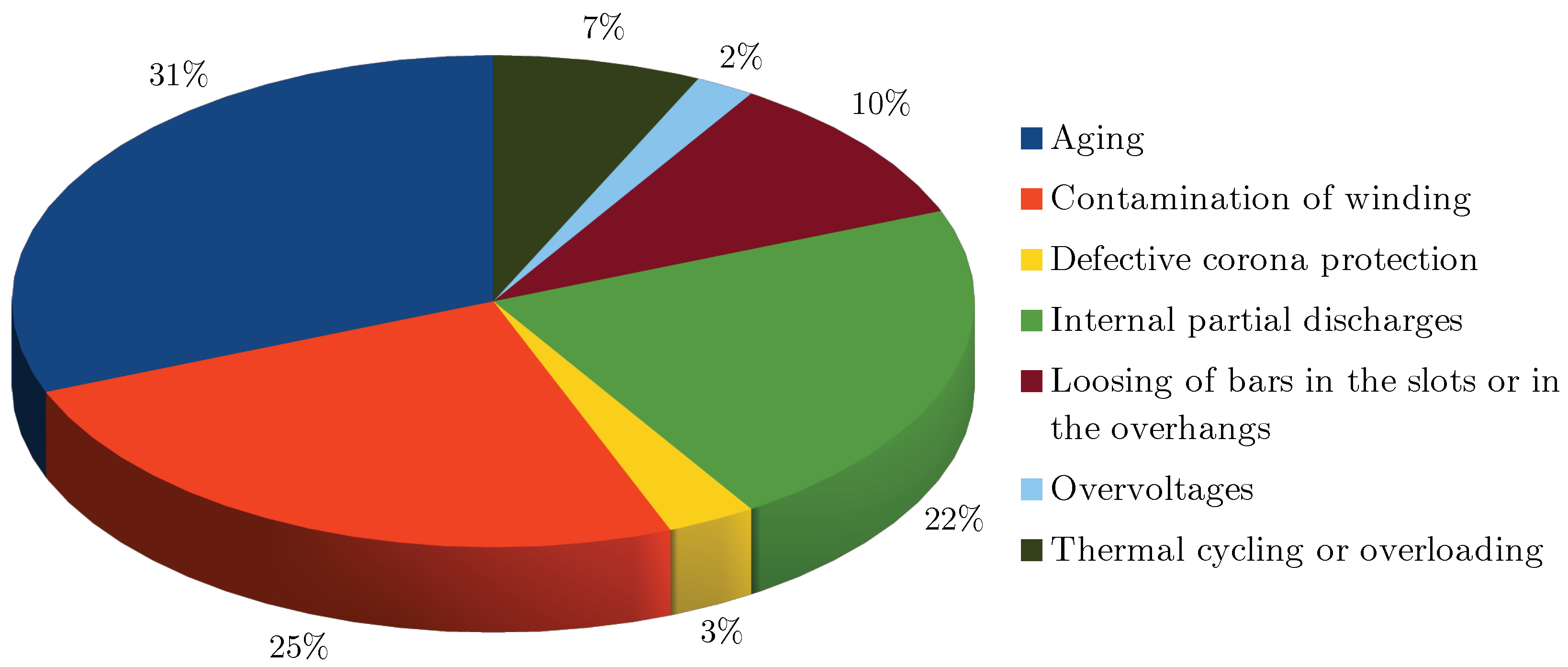
Figure 1.
Respective probabilities of factors leading to damages in insulation [
26].
Figure 1.
Respective probabilities of factors leading to damages in insulation [
26].
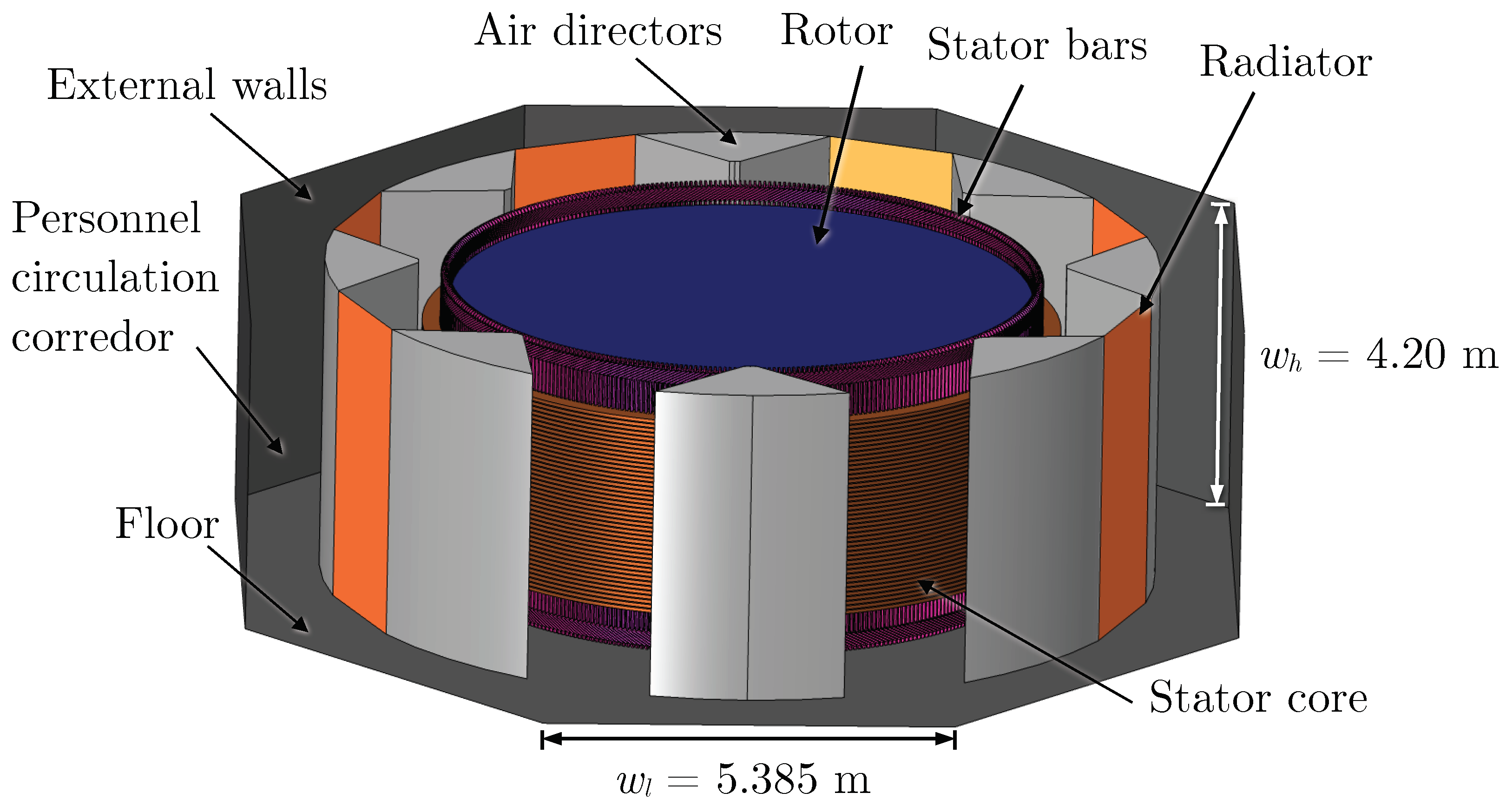
Figure 2.
Overview of the finite element model of the hydrogenerator: labeling of the structural parts. Wall height and width are provided.
Figure 2.
Overview of the finite element model of the hydrogenerator: labeling of the structural parts. Wall height and width are provided.
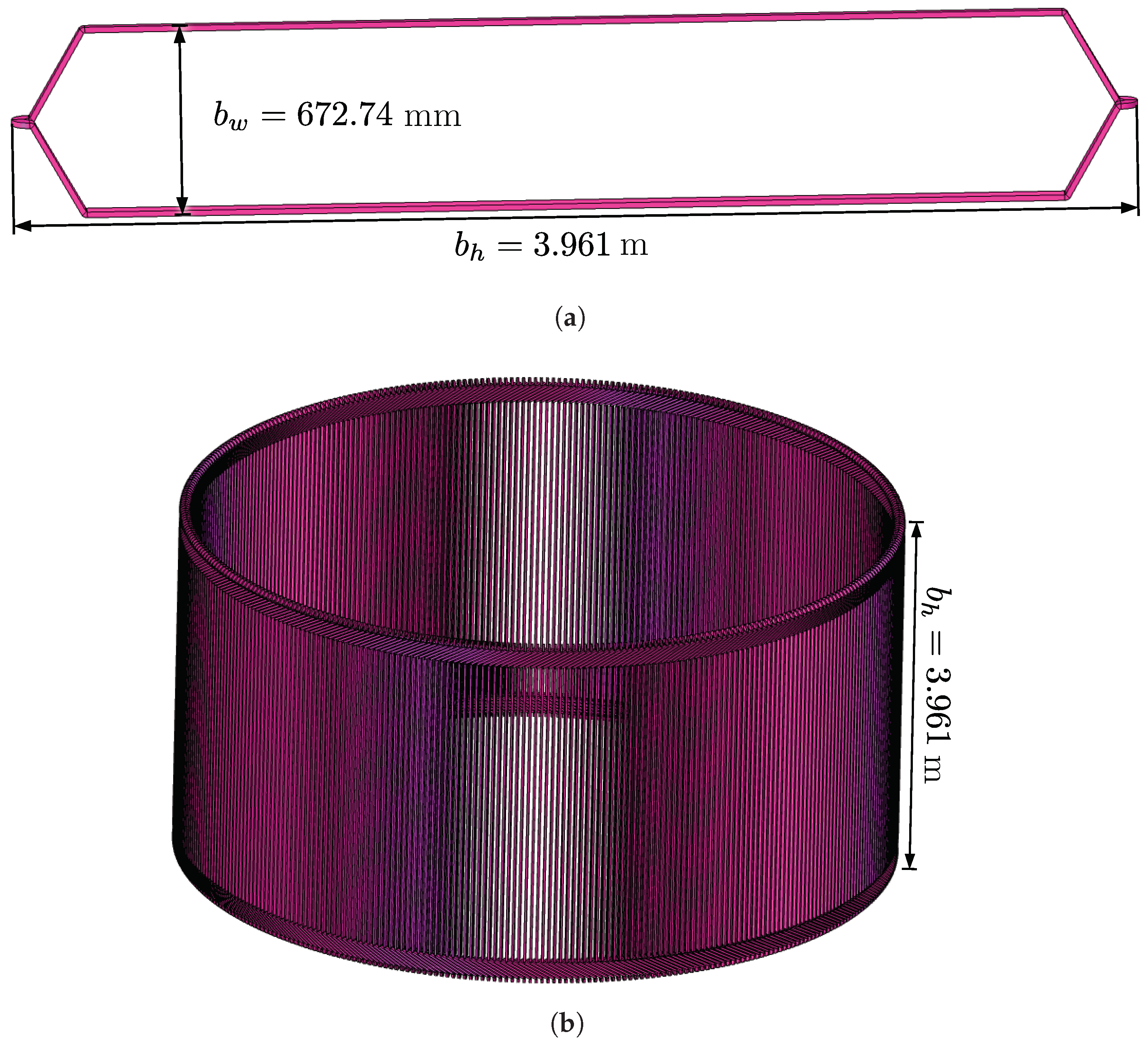
Figure 3.
Hydrogenerator stator bars and their dimensions: (a) the coil-type bar model and (b) all the 378 stator bars as arranged in the model of the hydrogenerator. Dimensions and are provided.
Figure 3.
Hydrogenerator stator bars and their dimensions: (a) the coil-type bar model and (b) all the 378 stator bars as arranged in the model of the hydrogenerator. Dimensions and are provided.
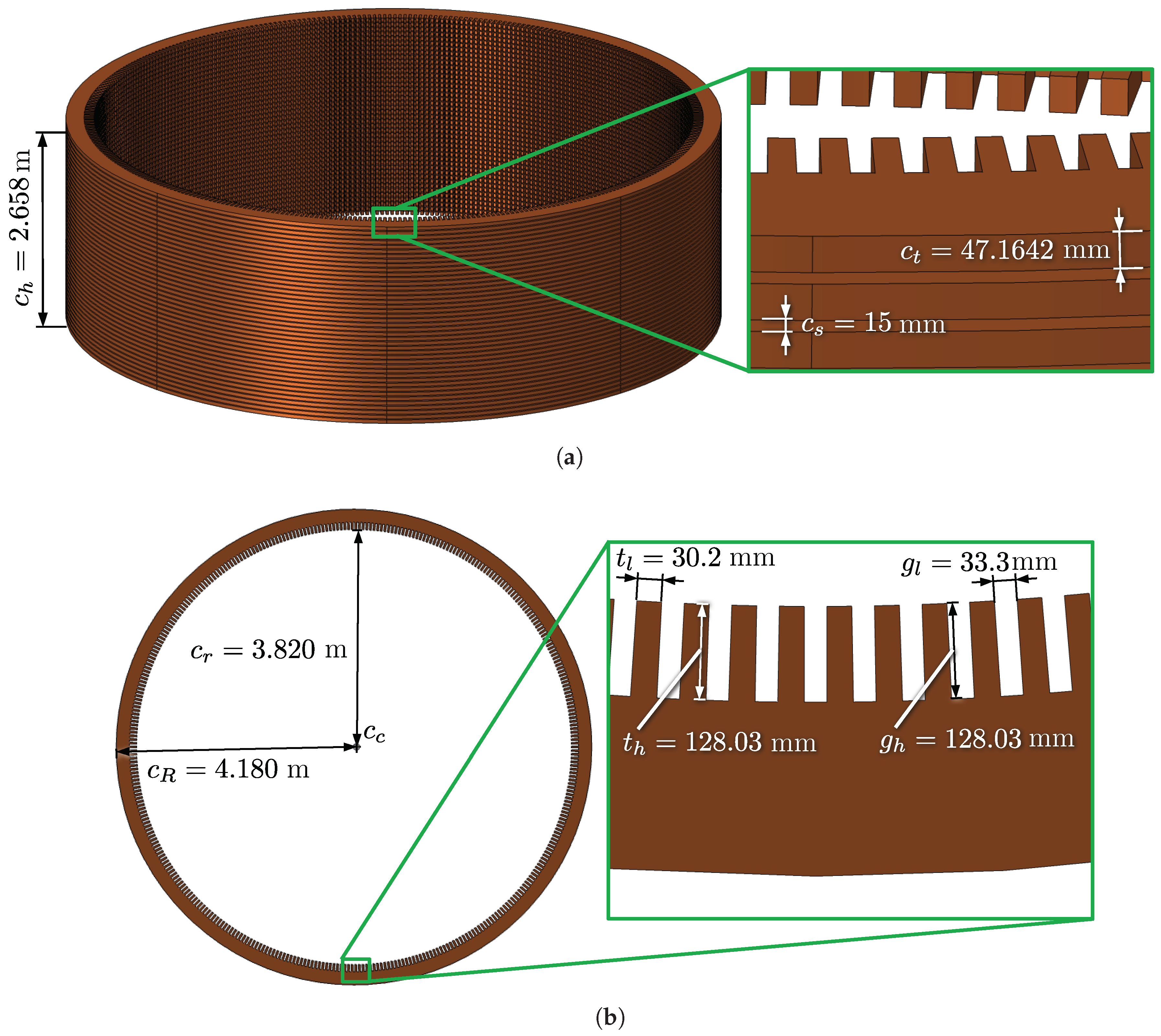
Figure 4.
Hydrogenerator stator core and its dimensions: (a) perspective view and (b) top view. Dimensions , and are given.
Figure 4.
Hydrogenerator stator core and its dimensions: (a) perspective view and (b) top view. Dimensions , and are given.
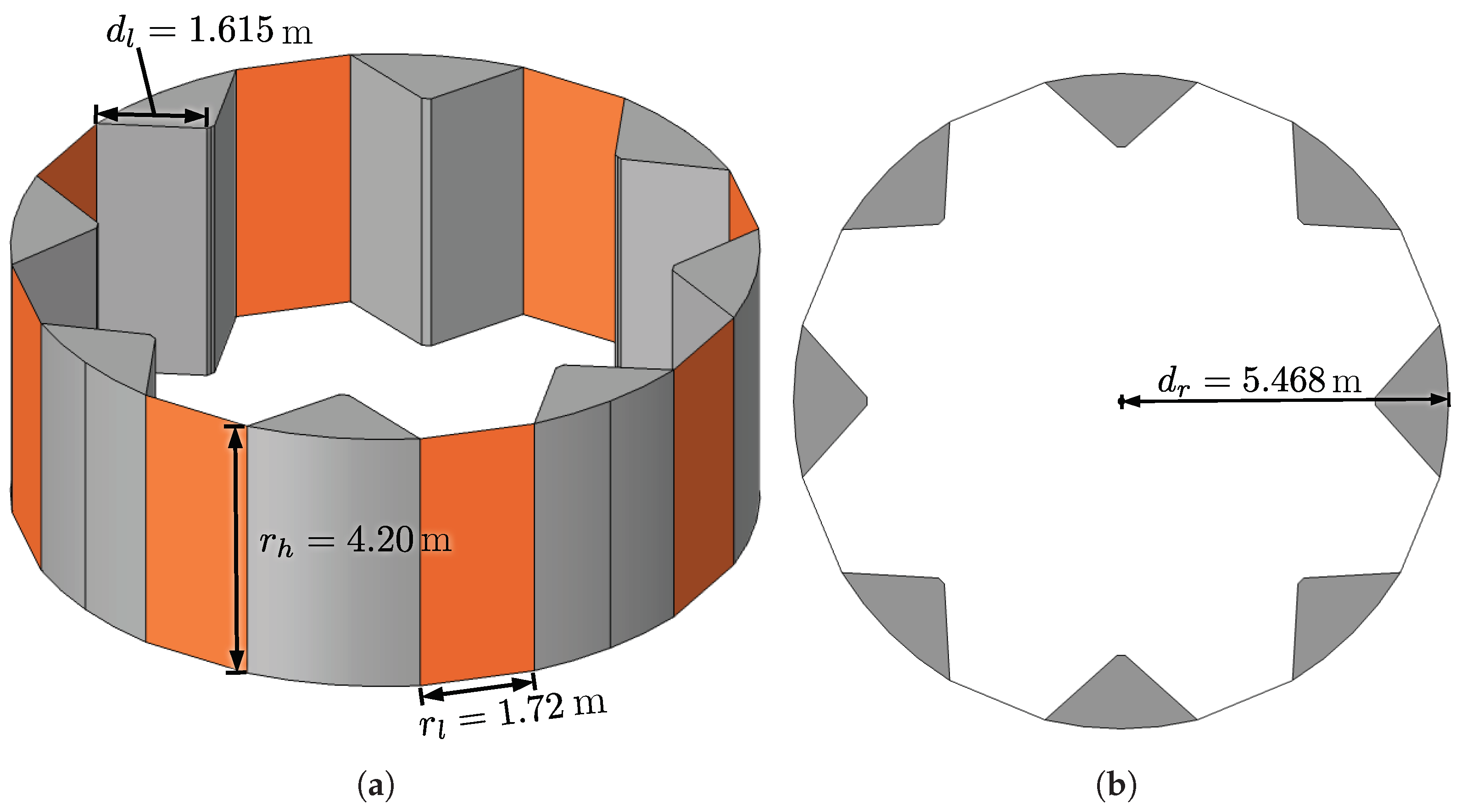
Figure 5.
Hydrogenerator air directors and radiator: (a) perspective view and (b) top view. The dimensions , , , and are given.
Figure 5.
Hydrogenerator air directors and radiator: (a) perspective view and (b) top view. The dimensions , , , and are given.
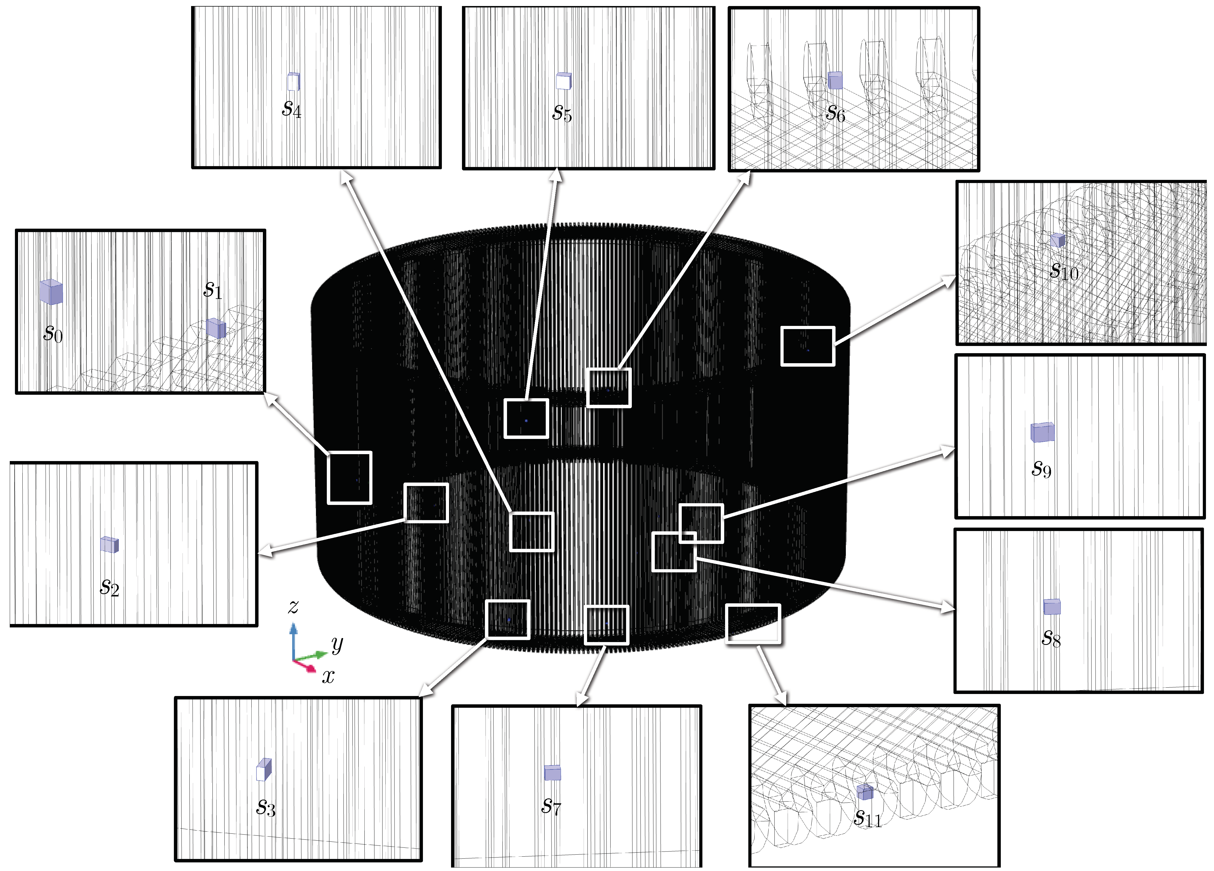
Figure 6.
Source positioning (and their labels) in hydrogenerator stator bars.
Figure 6.
Source positioning (and their labels) in hydrogenerator stator bars.
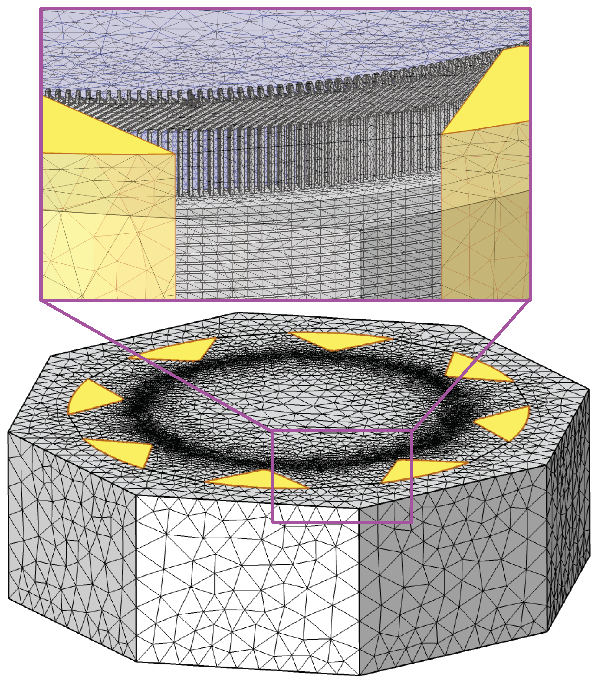
Figure 7.
Overview of the finite element mesh conceived for representing the hydrogenerator structure. Yellowish regions are air directors.
Figure 7.
Overview of the finite element mesh conceived for representing the hydrogenerator structure. Yellowish regions are air directors.
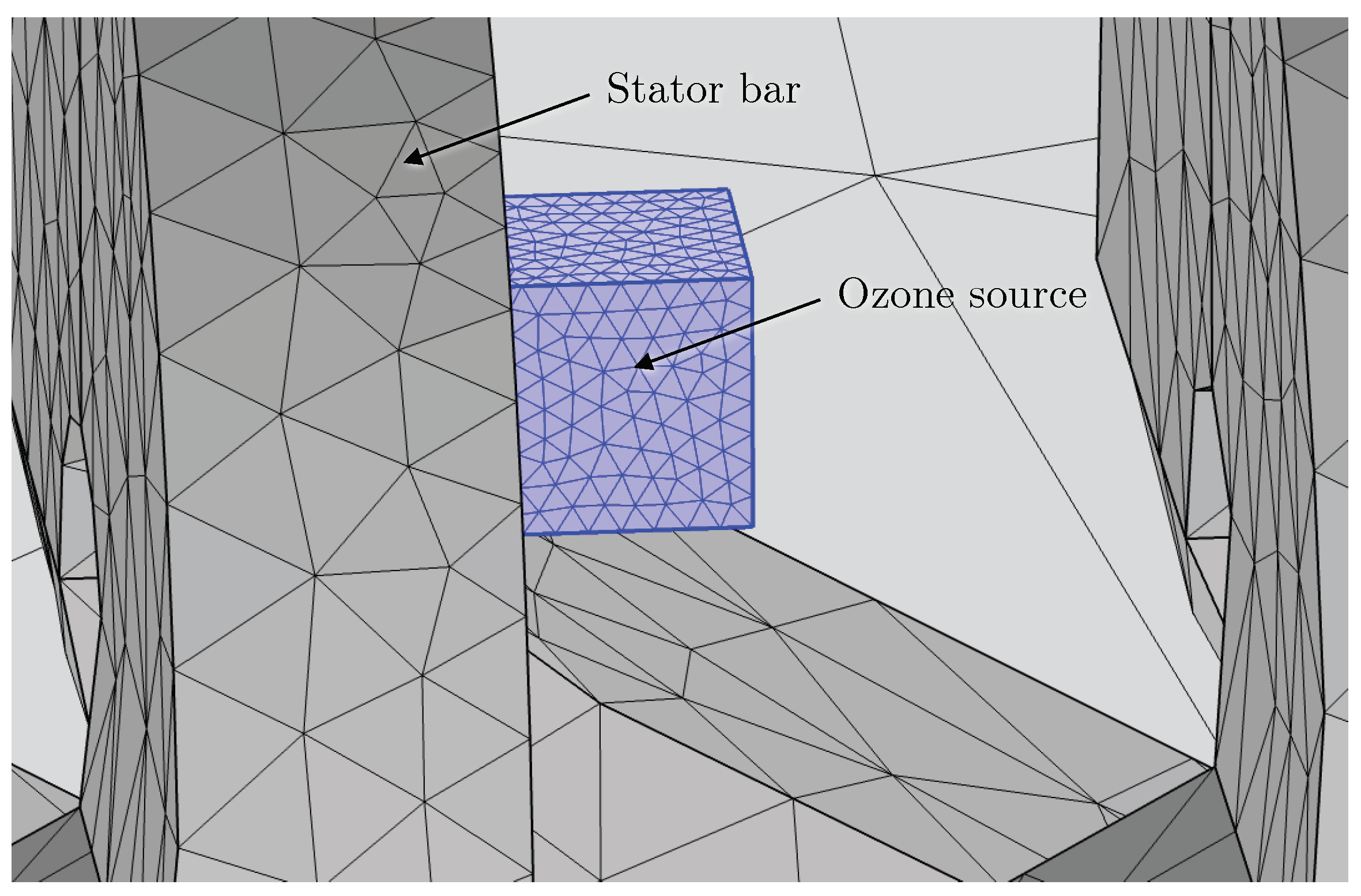
Figure 8.
Part of the conceived computational mesh for representing ozone sources (highlighted in blue) and stator bars.
Figure 8.
Part of the conceived computational mesh for representing ozone sources (highlighted in blue) and stator bars.
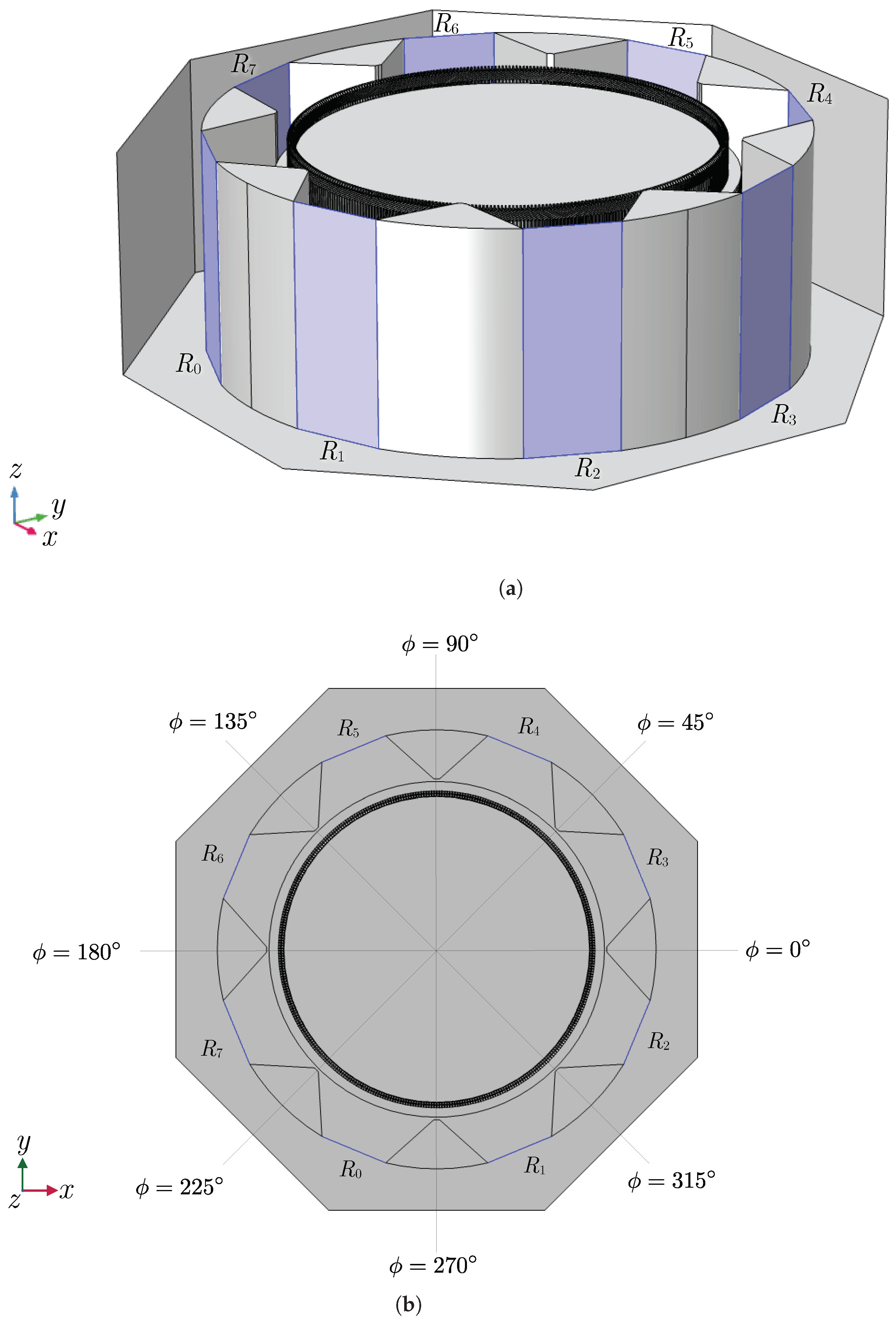
Figure 9.
Labels of each hydrogenerator radiator and angles of reference: (a) perspective view and (b) top view. Radiators are seen with shades of blue.
Figure 9.
Labels of each hydrogenerator radiator and angles of reference: (a) perspective view and (b) top view. Radiators are seen with shades of blue.
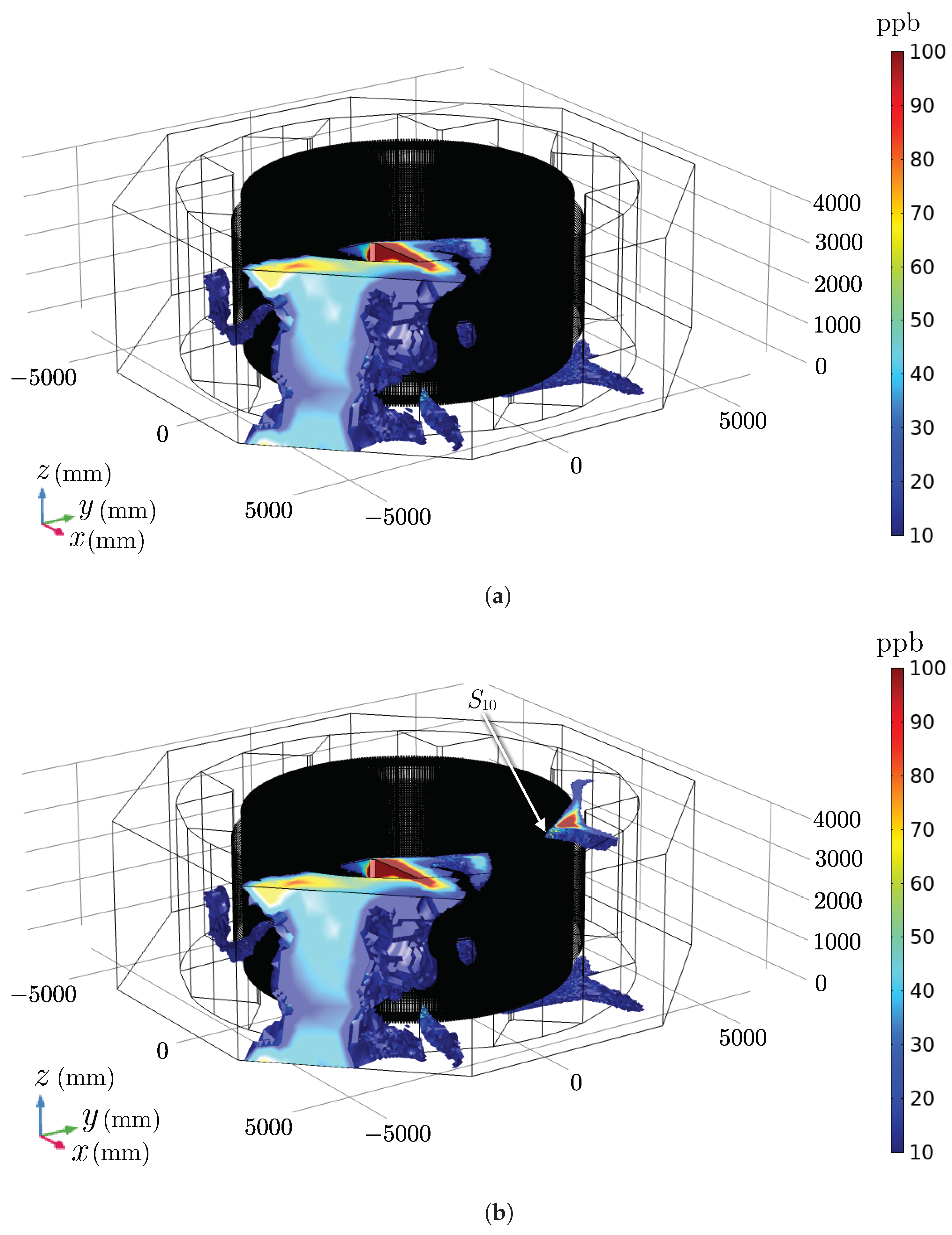
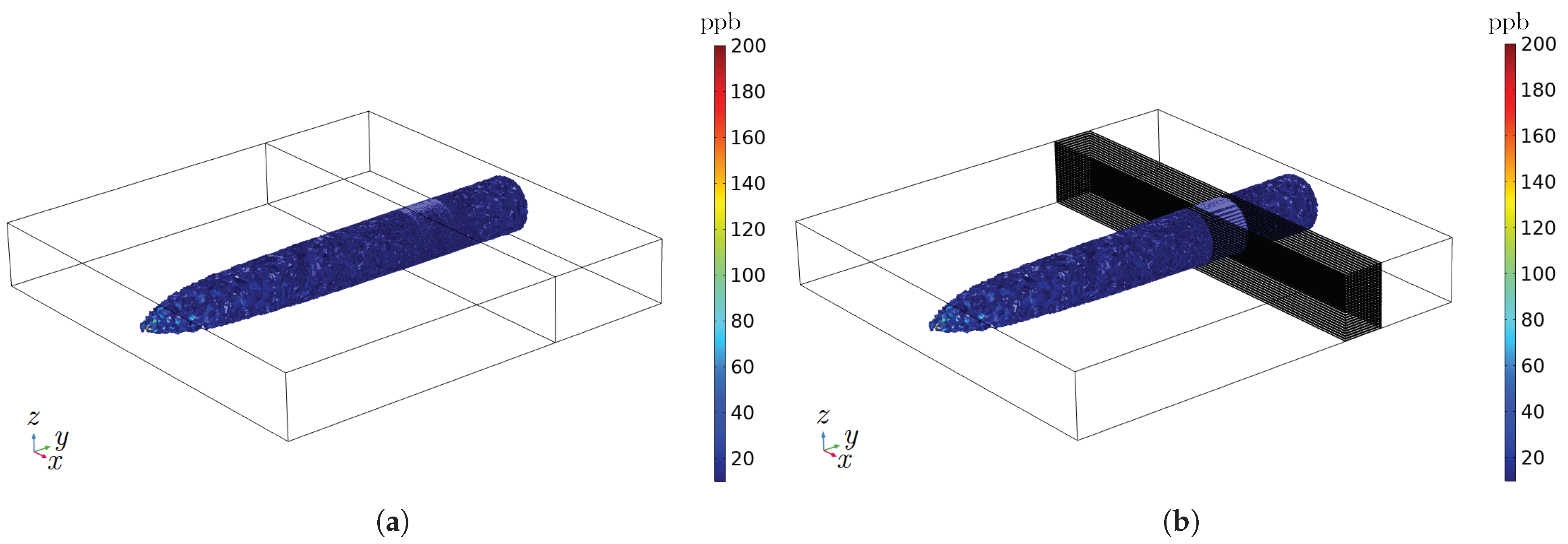
Figure 10.
Ozone concentration (ppb) overview in the numerical model of the hydrogenerator for simulations (a) A and (b) B (with source additionally activated).
Figure 10.
Ozone concentration (ppb) overview in the numerical model of the hydrogenerator for simulations (a) A and (b) B (with source additionally activated).
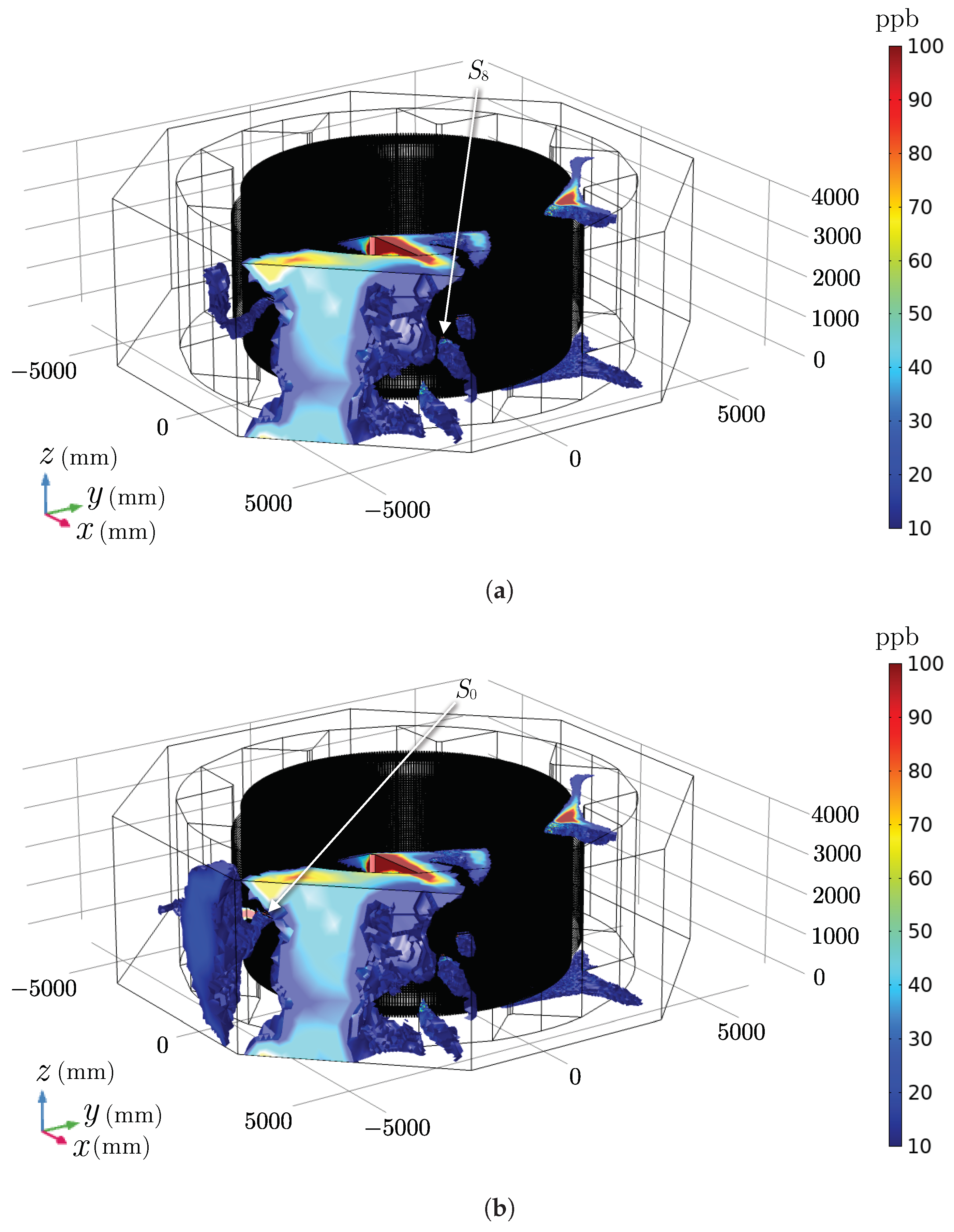
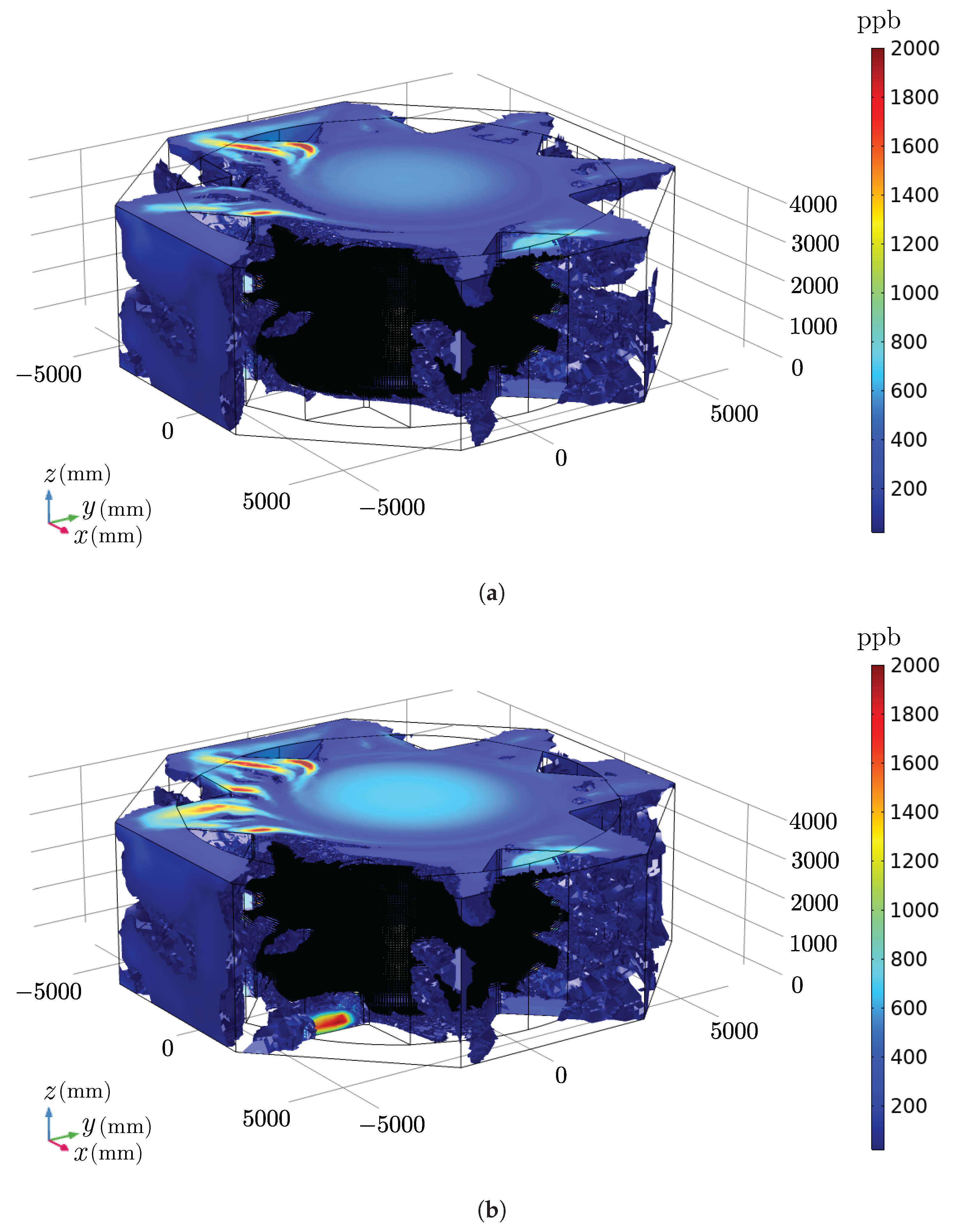
Figure 11.
Overview of ozone concentration (ppb) in numerical model of hydrogenerator in simulations: (a) C (source additionally activated) and (b) D (source additionally activated).
Figure 11.
Overview of ozone concentration (ppb) in numerical model of hydrogenerator in simulations: (a) C (source additionally activated) and (b) D (source additionally activated).
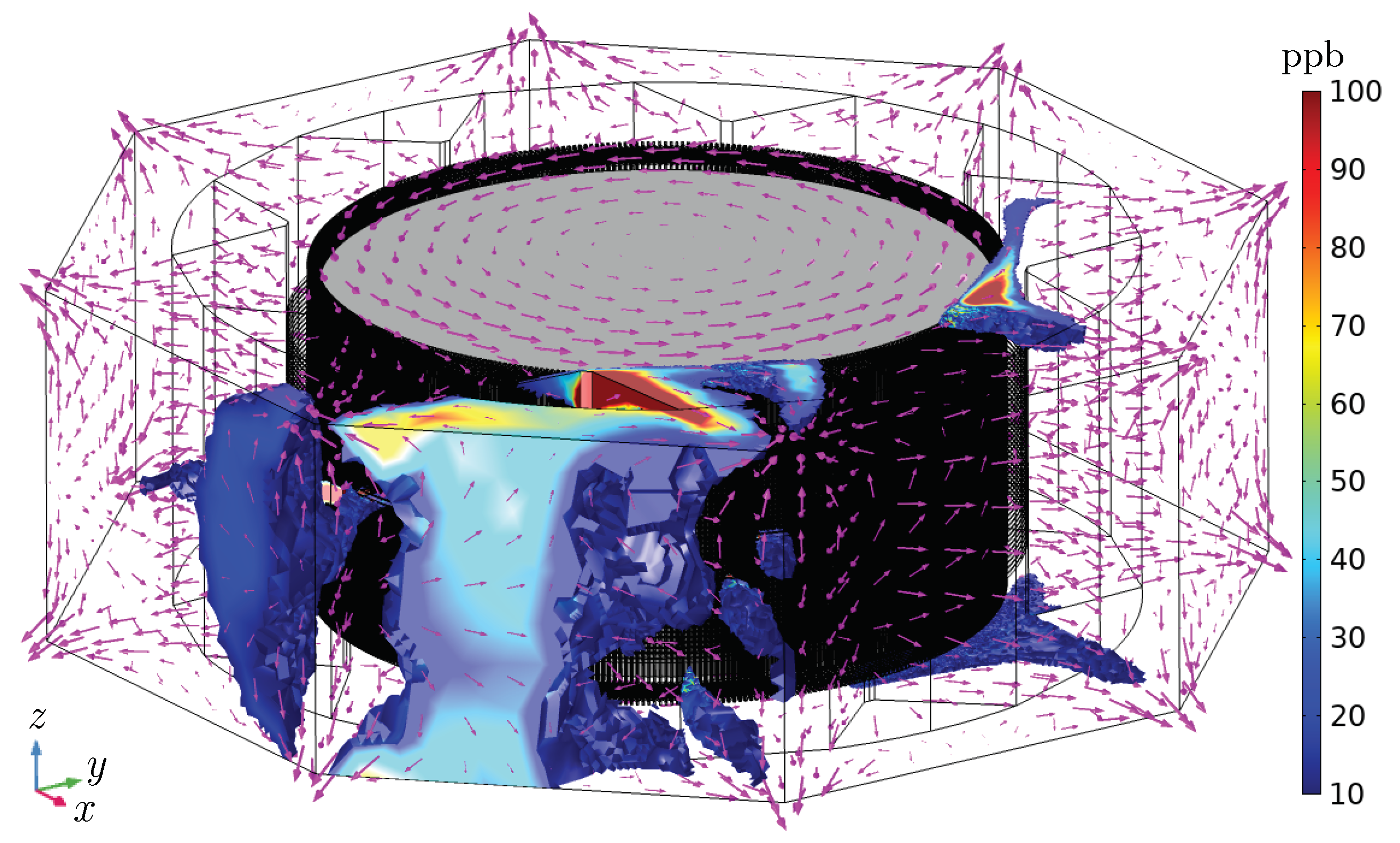
Figure 12.
Ozone concentration (ppb) overview in the numerical model of the hydrogenerator for simulation D (including vector velocity field with log-scale vector sizes).
Figure 12.
Ozone concentration (ppb) overview in the numerical model of the hydrogenerator for simulation D (including vector velocity field with log-scale vector sizes).
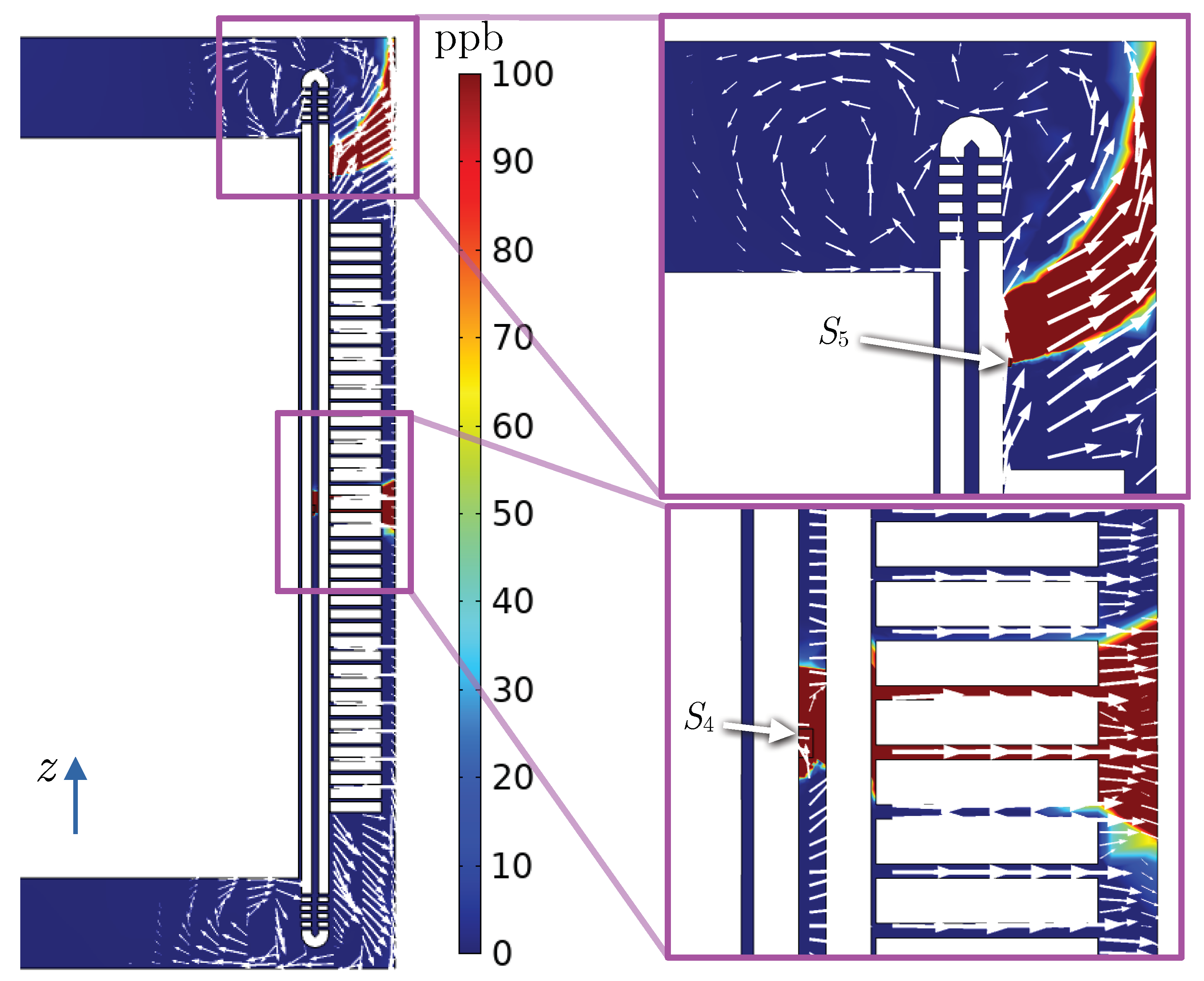
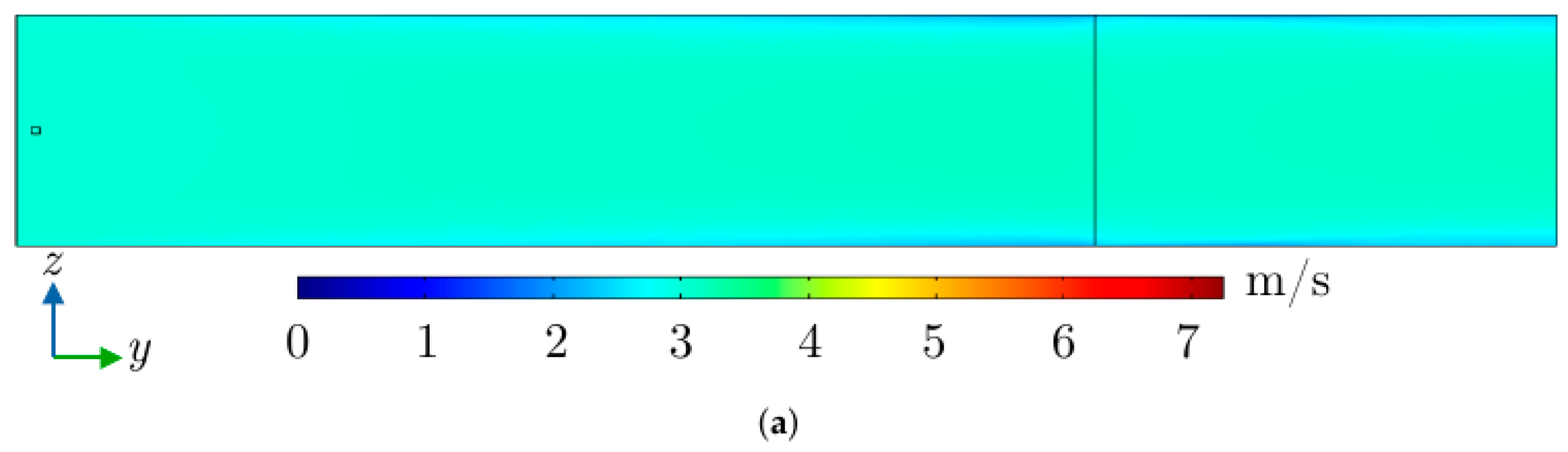
Figure 13.
Ozone distribution (ppb) and velocity field on the vertical plane perpendicular to sources and (simulation D, °).
Figure 13.
Ozone distribution (ppb) and velocity field on the vertical plane perpendicular to sources and (simulation D, °).
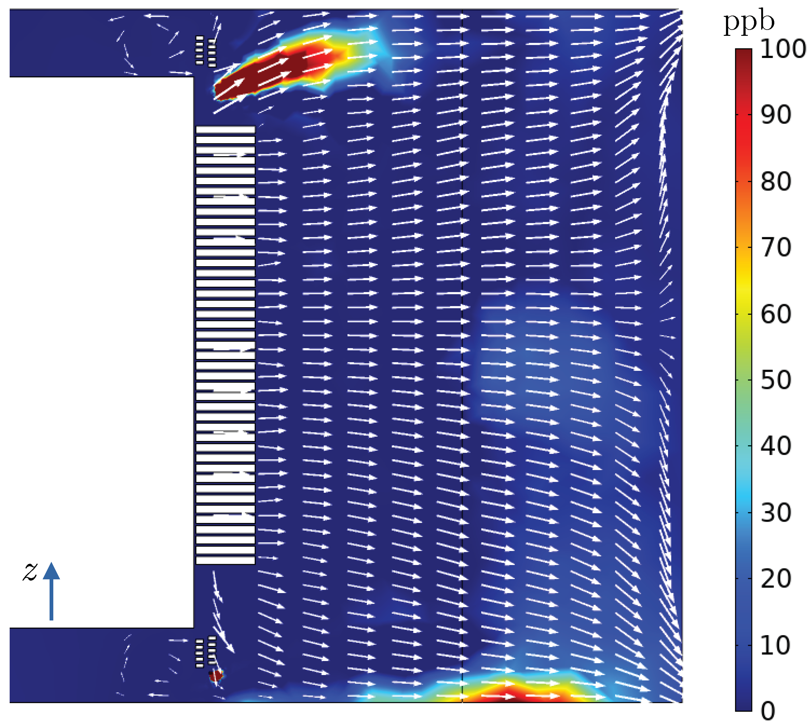
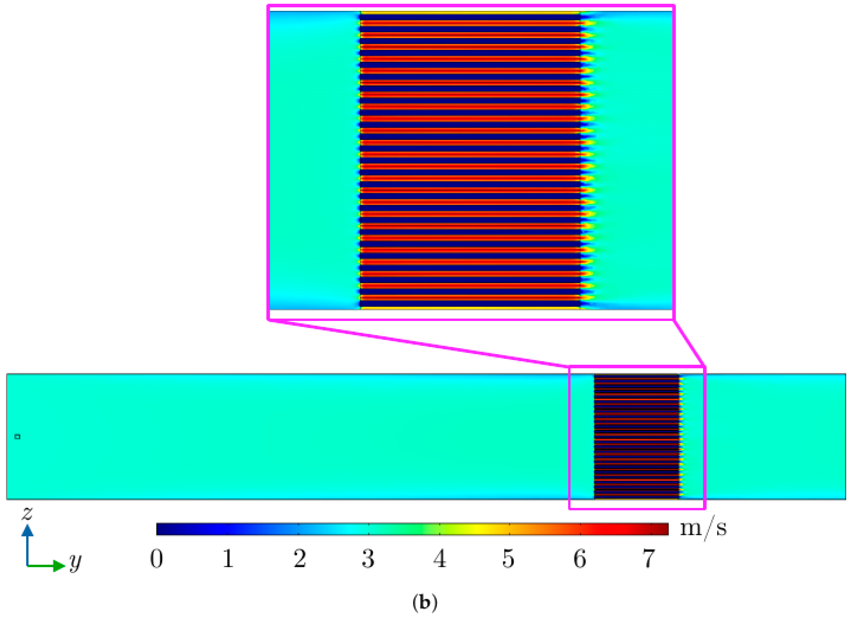
Figure 14.
Ozone distribution (ppb) and velocity field on the vertical plane perpendicular to radiator (simulation D, °).
Figure 14.
Ozone distribution (ppb) and velocity field on the vertical plane perpendicular to radiator (simulation D, °).
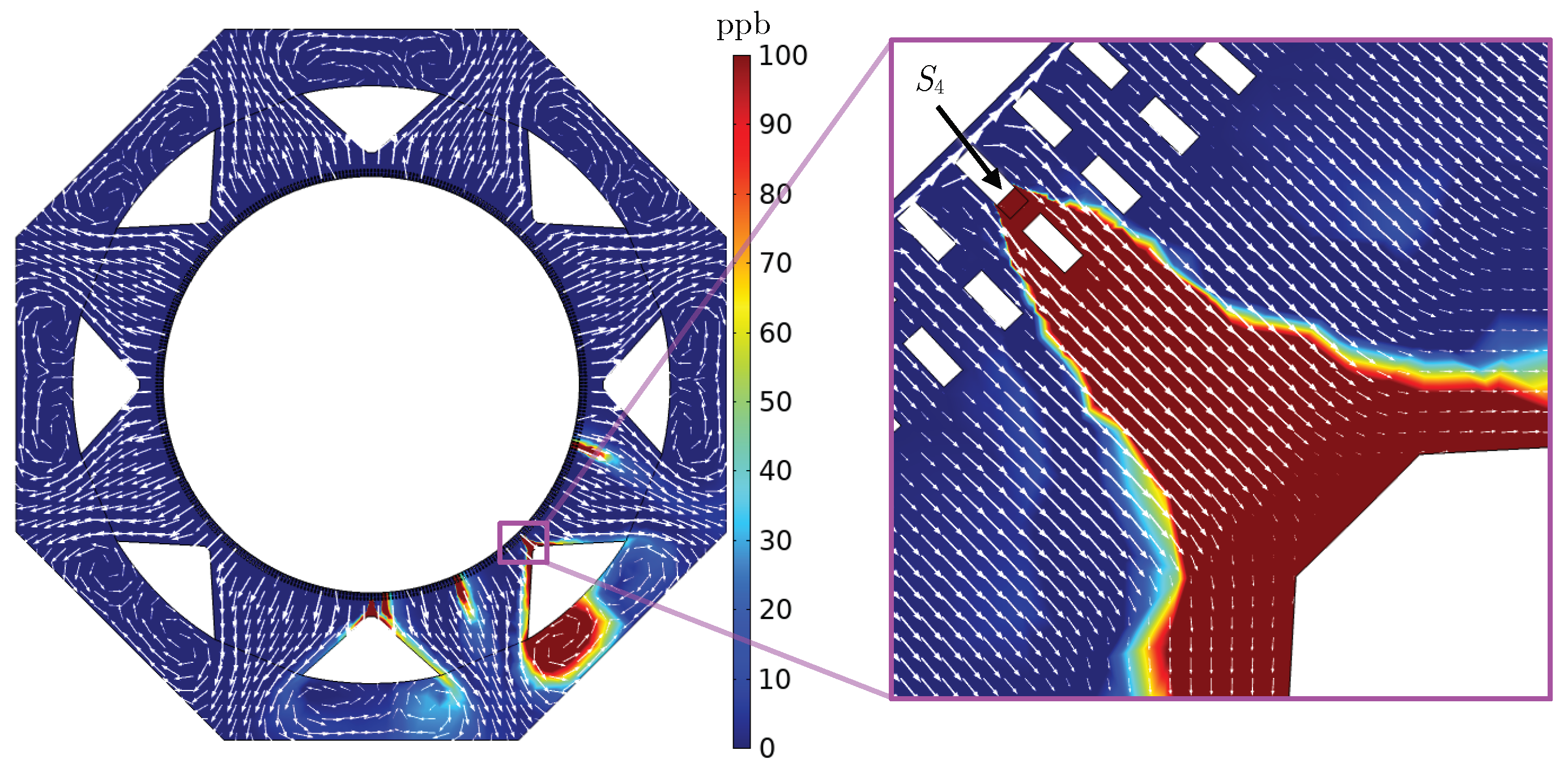
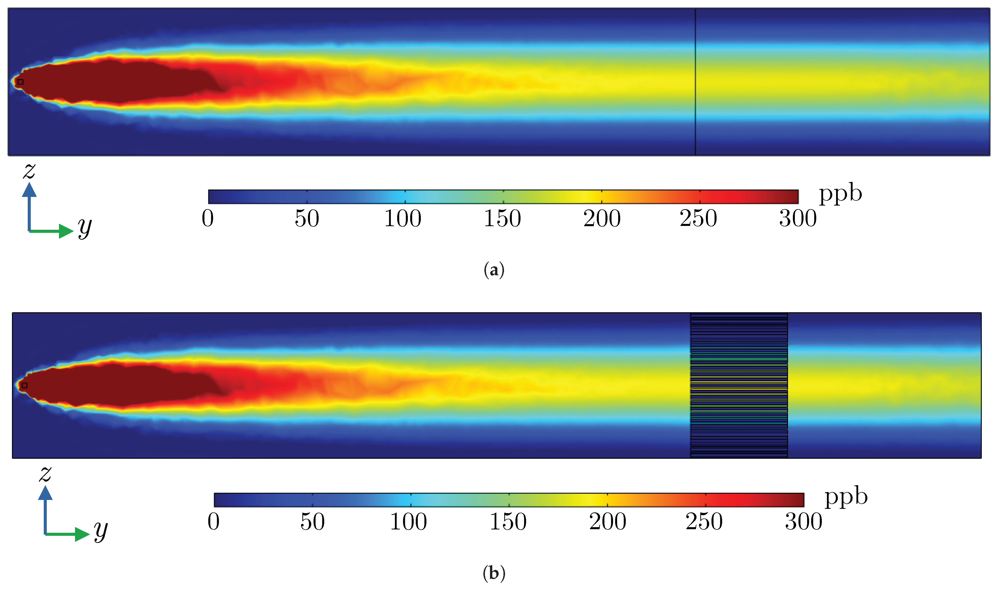
Figure 15.
Ozone distribution (ppb) and velocity field on the horizontal plane perpendicular to source (simulation D, m).
Figure 15.
Ozone distribution (ppb) and velocity field on the horizontal plane perpendicular to source (simulation D, m).
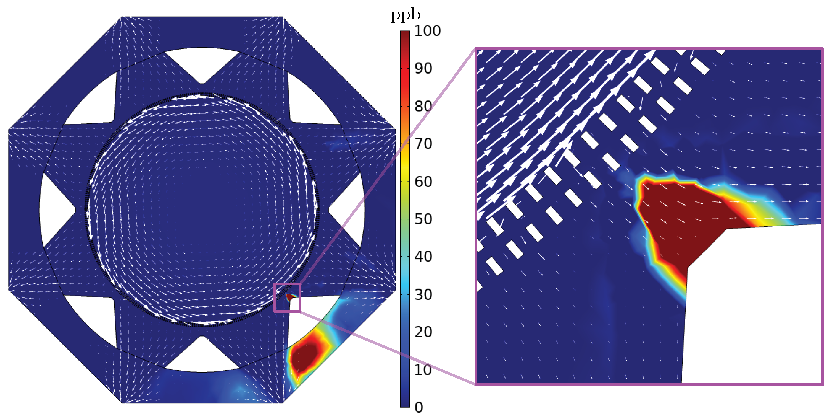
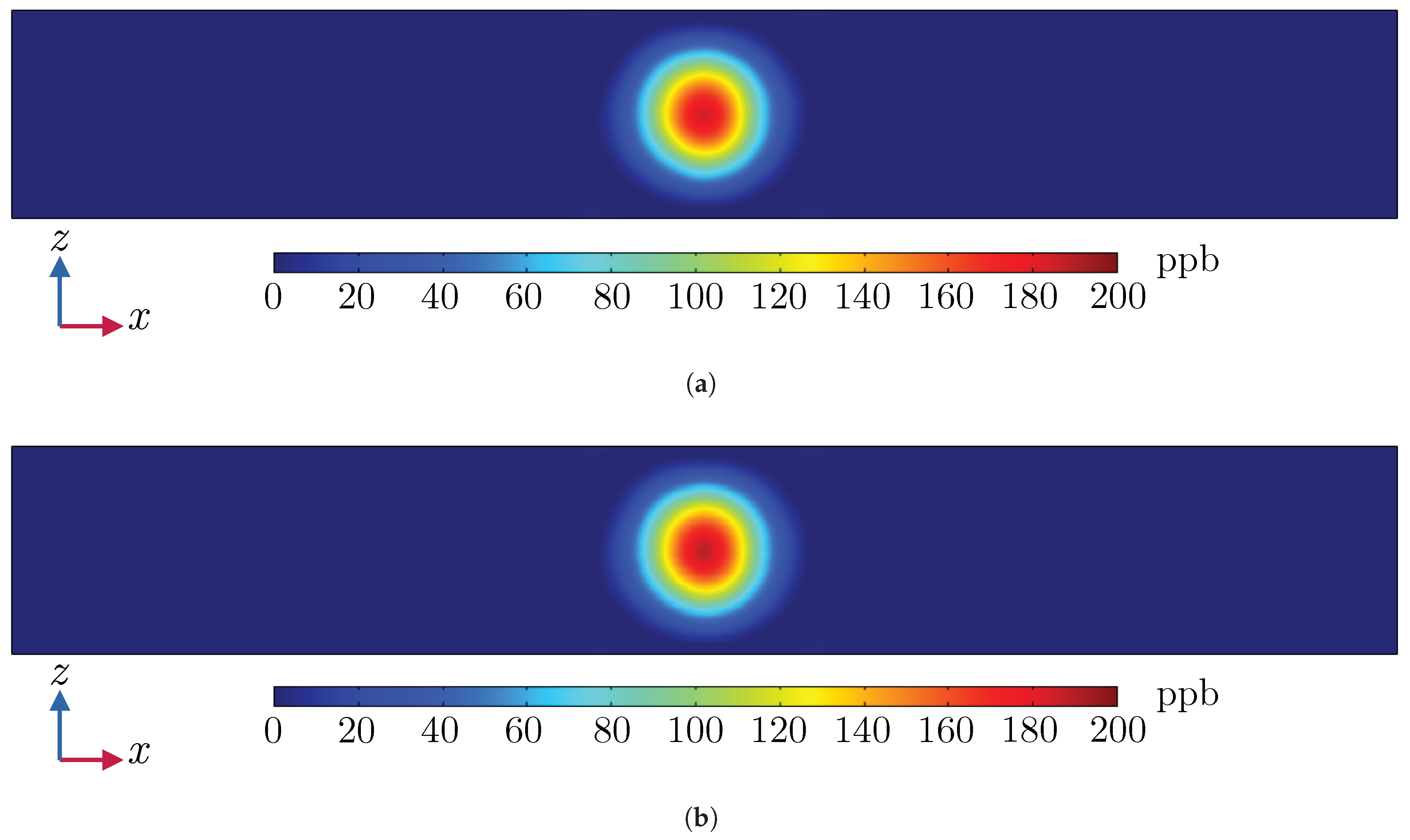
Figure 16.
Ozone distribution (ppb) and velocity field on a horizontal plane at the top region of the hydrogenerator (simulation D, m).
Figure 16.
Ozone distribution (ppb) and velocity field on a horizontal plane at the top region of the hydrogenerator (simulation D, m).
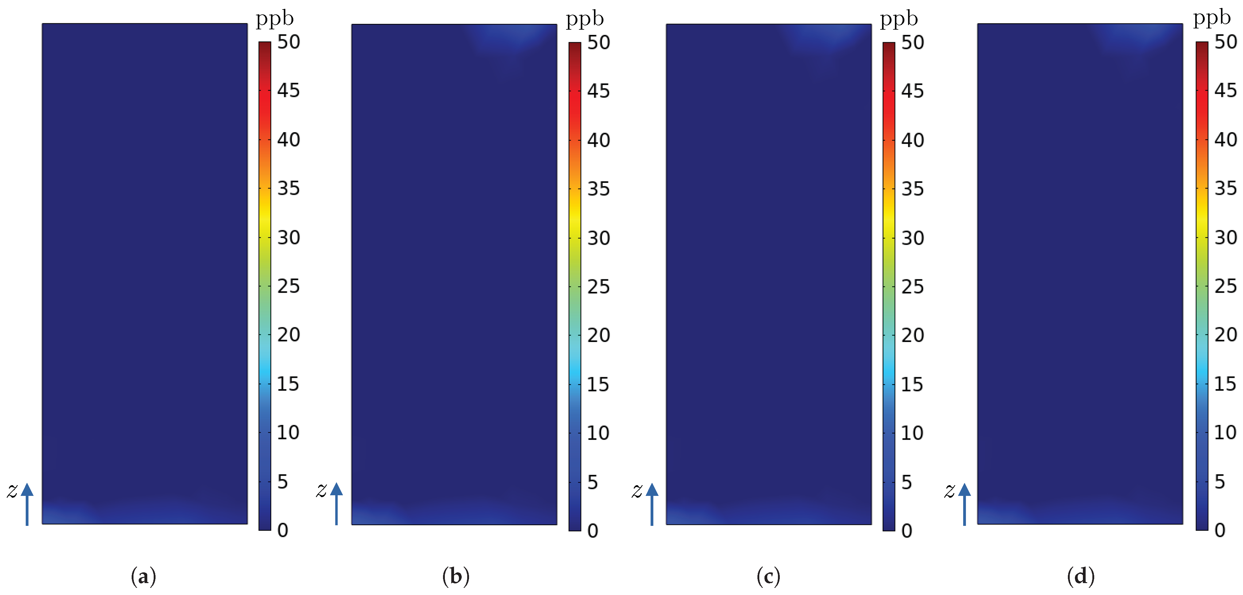
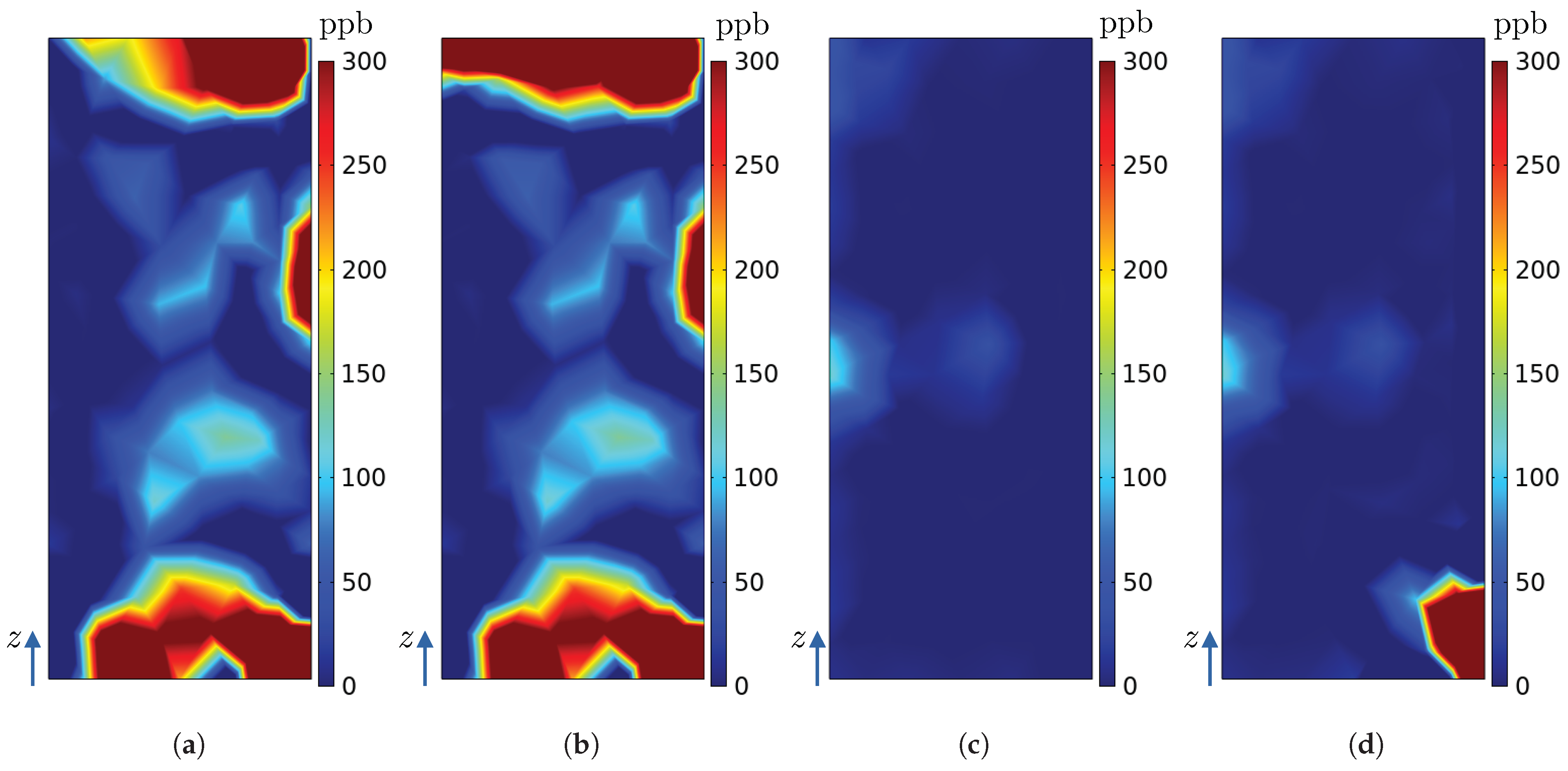
Figure 17.
Ozone concentrations (ppb) on the surface of radiator in the numerical model of the hydrogenerator for simulations (a) A, (b) B, (c) C and (d) D.
Figure 17.
Ozone concentrations (ppb) on the surface of radiator in the numerical model of the hydrogenerator for simulations (a) A, (b) B, (c) C and (d) D.
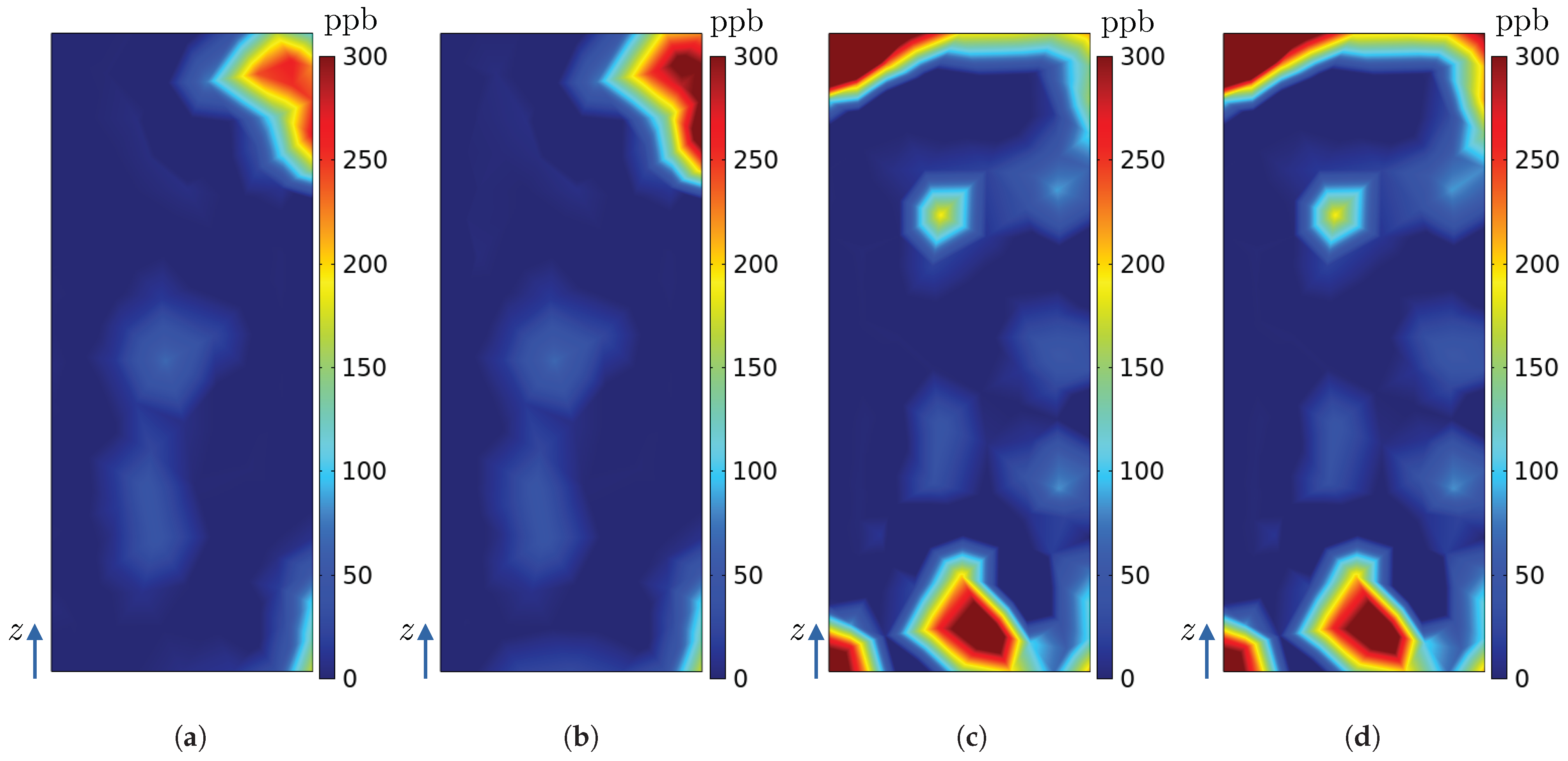
Figure 18.
Ozone concentrations (ppb) on the surface of radiator in numerical model of the hydrogenerator for simulations (a) A, (b) B, (c) C and (d) D.
Figure 18.
Ozone concentrations (ppb) on the surface of radiator in numerical model of the hydrogenerator for simulations (a) A, (b) B, (c) C and (d) D.
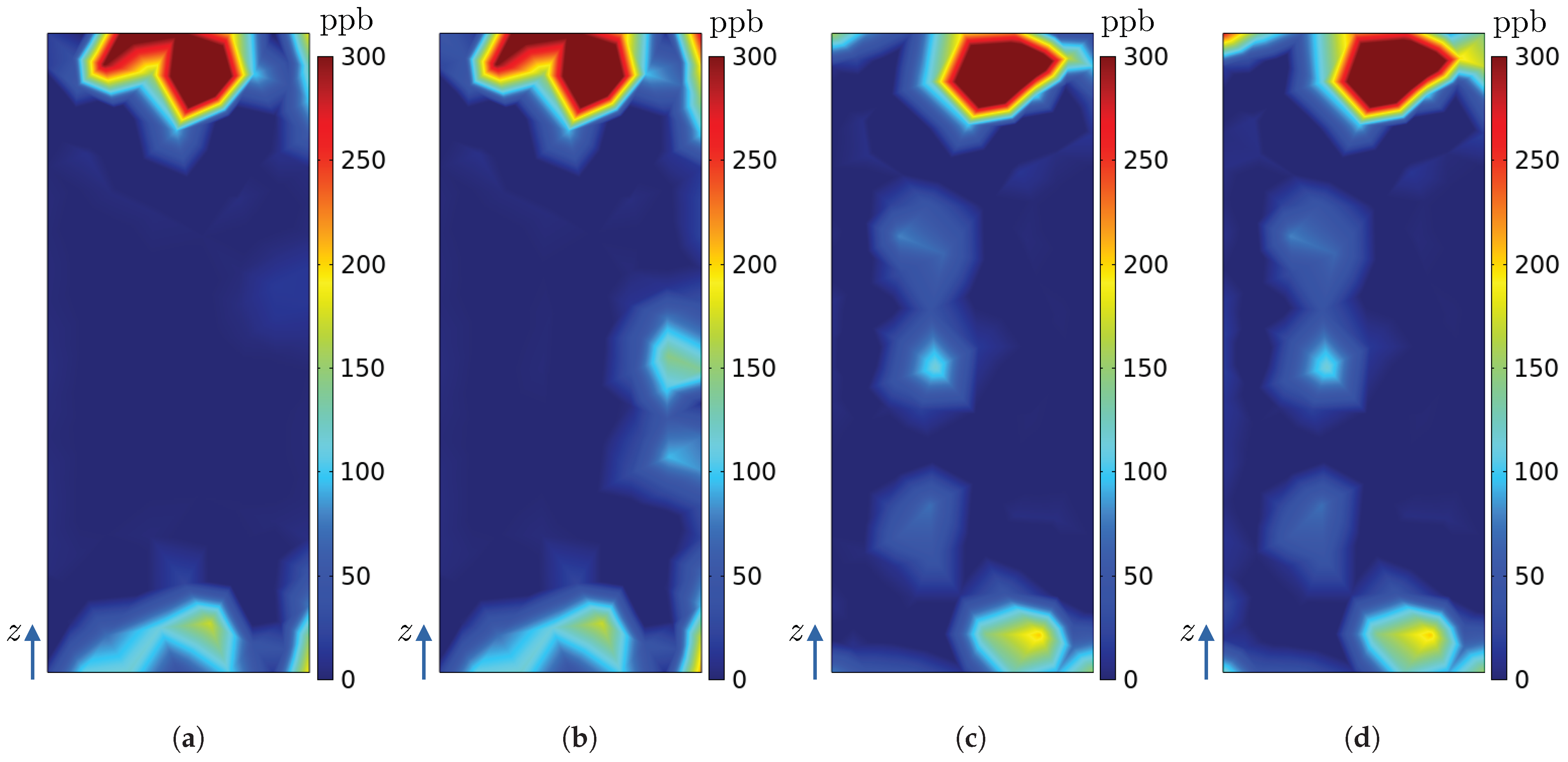
Figure 19.
Ozone concentrations (ppb) on the surface of radiator in the numerical model of the hydrogenerator for simulations (a) A, (b) B, (c) C, and (d) D.
Figure 19.
Ozone concentrations (ppb) on the surface of radiator in the numerical model of the hydrogenerator for simulations (a) A, (b) B, (c) C, and (d) D.
Figure 20.
Ozone concentrations (ppb) on the surface of the radiator in numerical model of the hydrogenerator for simulations (a) A, (b) B, (c) C, and (d) D.
Figure 20.
Ozone concentrations (ppb) on the surface of the radiator in numerical model of the hydrogenerator for simulations (a) A, (b) B, (c) C, and (d) D.
Figure 21.
Ozone concentrations (ppb) on the surface of the radiator in the numerical model of the hydrogenerator for simulations (a) A, (b) B, (c) C, and (d) D.
Figure 21.
Ozone concentrations (ppb) on the surface of the radiator in the numerical model of the hydrogenerator for simulations (a) A, (b) B, (c) C, and (d) D.
Figure 22.
Influence of sources (°) to (°) in simulations (a) E and (b) F.
Figure 22.
Influence of sources (°) to (°) in simulations (a) E and (b) F.
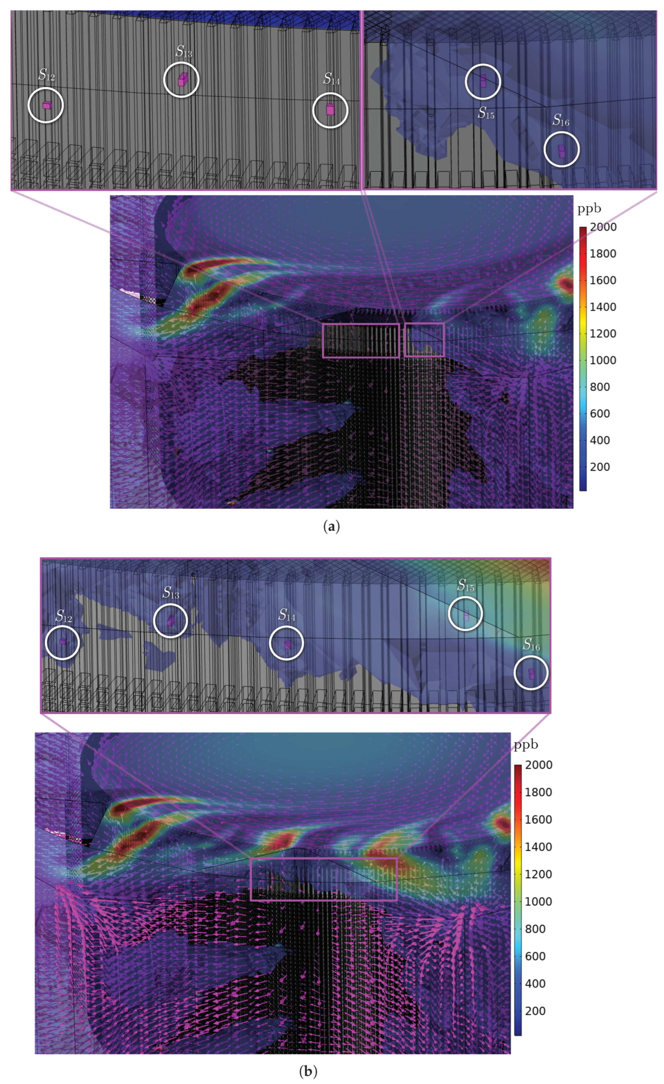
Figure 23.
Localized influence in the region of sources (°) and (°) in simulations (a) E and (b) F.
Figure 23.
Localized influence in the region of sources (°) and (°) in simulations (a) E and (b) F.
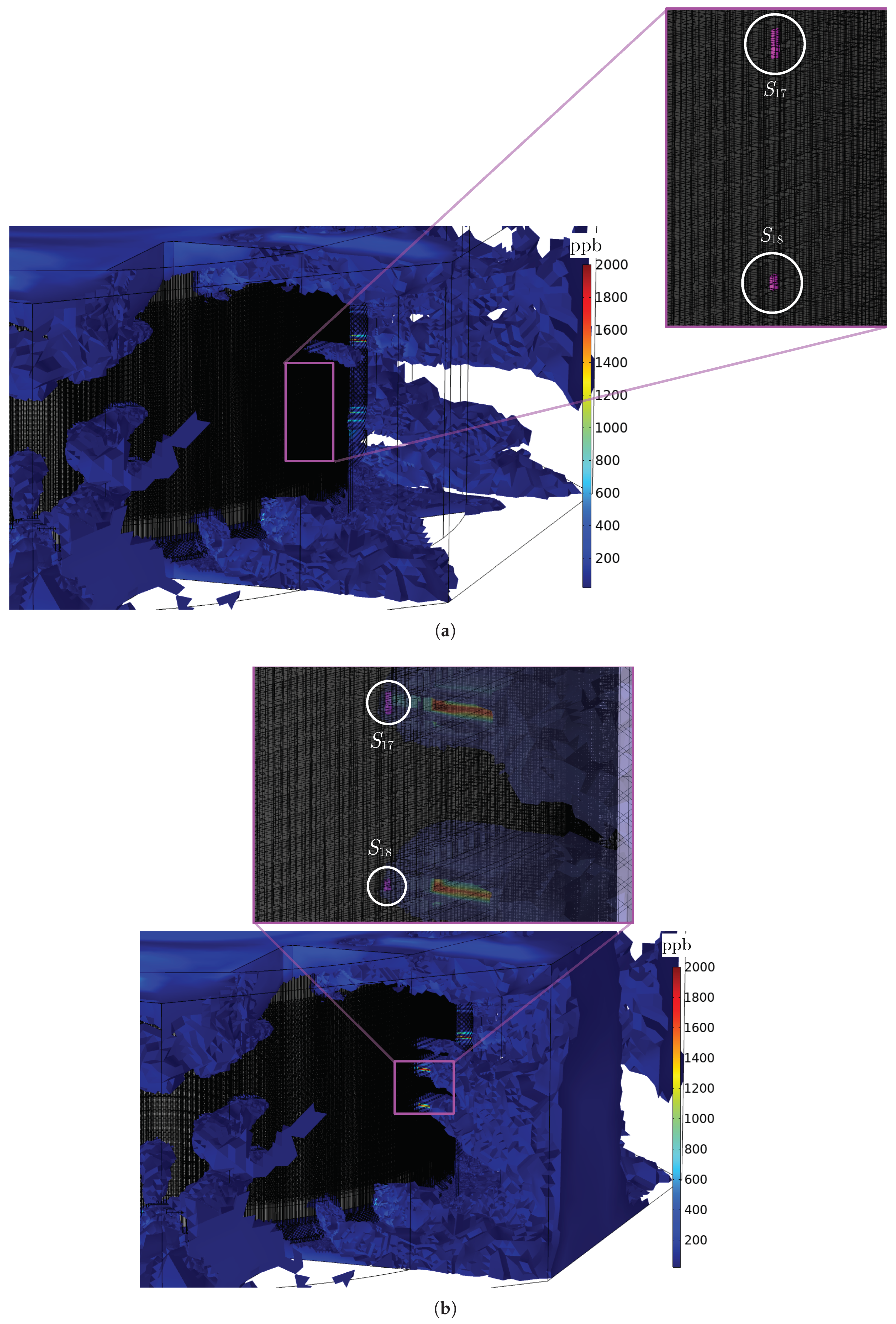
Figure 24.
Localized influence in the region of sources (°) and (°) in simulations (a) E and (b) F.
Figure 24.
Localized influence in the region of sources (°) and (°) in simulations (a) E and (b) F.
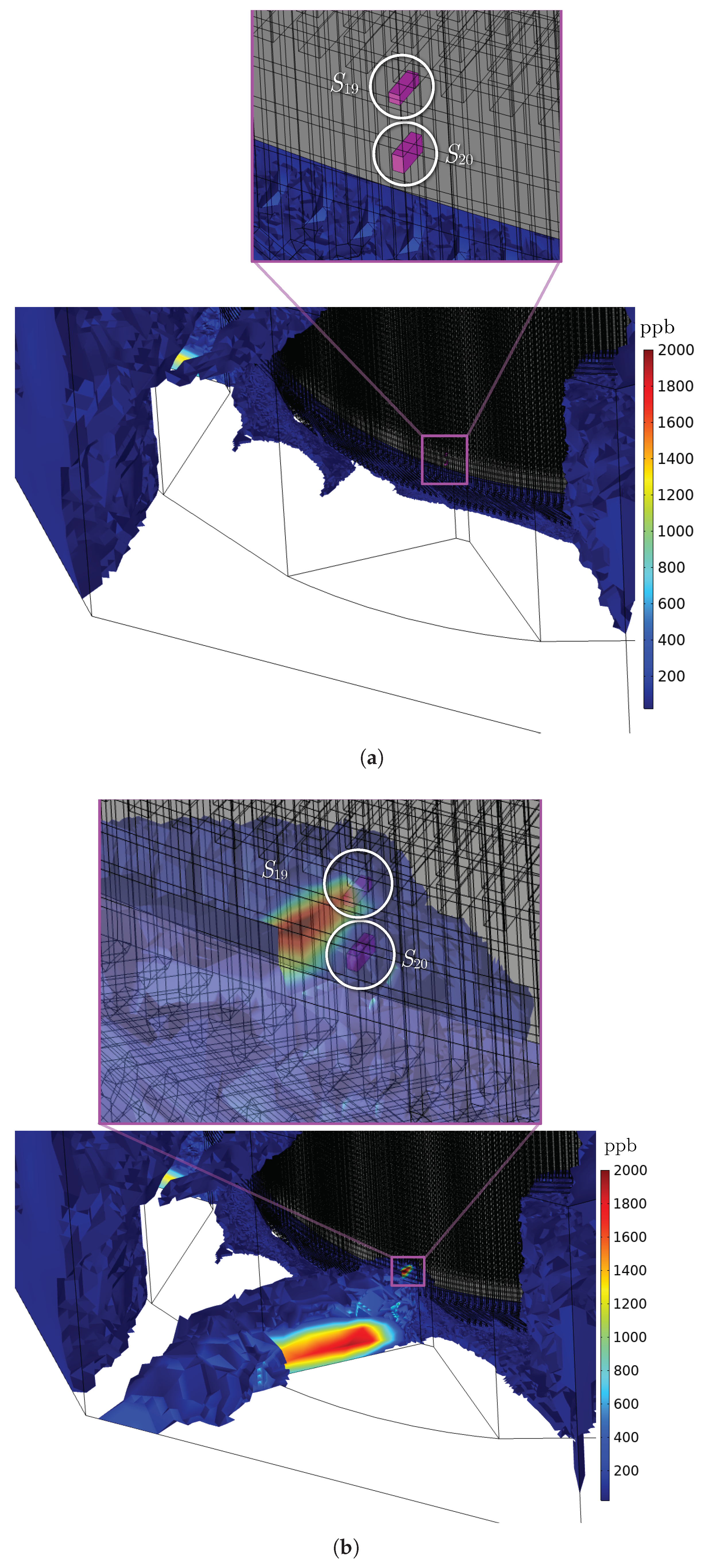
Figure 25.
Perspective view of ozone concentration (ppb) in numerical model of hydrogenerator in simulations (a) E and (b) F.
Figure 25.
Perspective view of ozone concentration (ppb) in numerical model of hydrogenerator in simulations (a) E and (b) F.
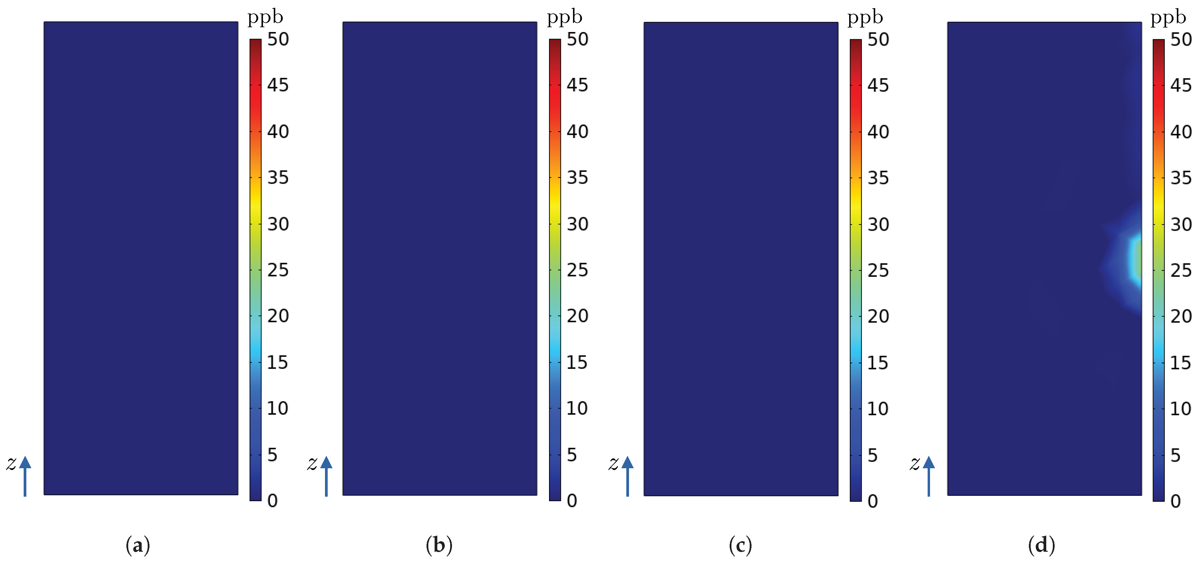
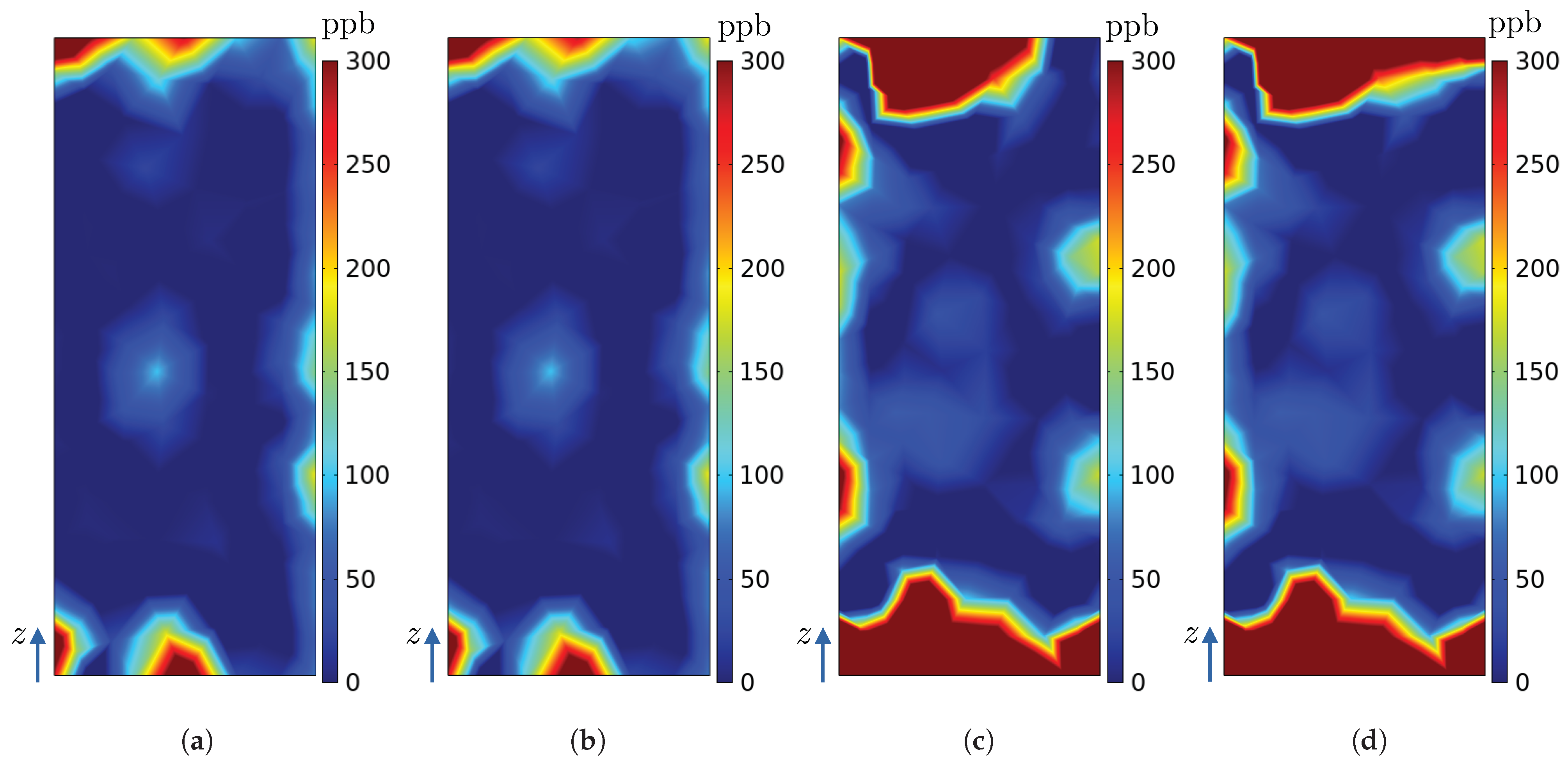
Figure 26.
Ozone concentration (ppb) on the surfaces of the radiators and in the numerical model of the hydrogenerator: (a) (simulation E), (b) (simulation F), (c) (simulation E), and (d) (simulation F).
Figure 26.
Ozone concentration (ppb) on the surfaces of the radiators and in the numerical model of the hydrogenerator: (a) (simulation E), (b) (simulation F), (c) (simulation E), and (d) (simulation F).
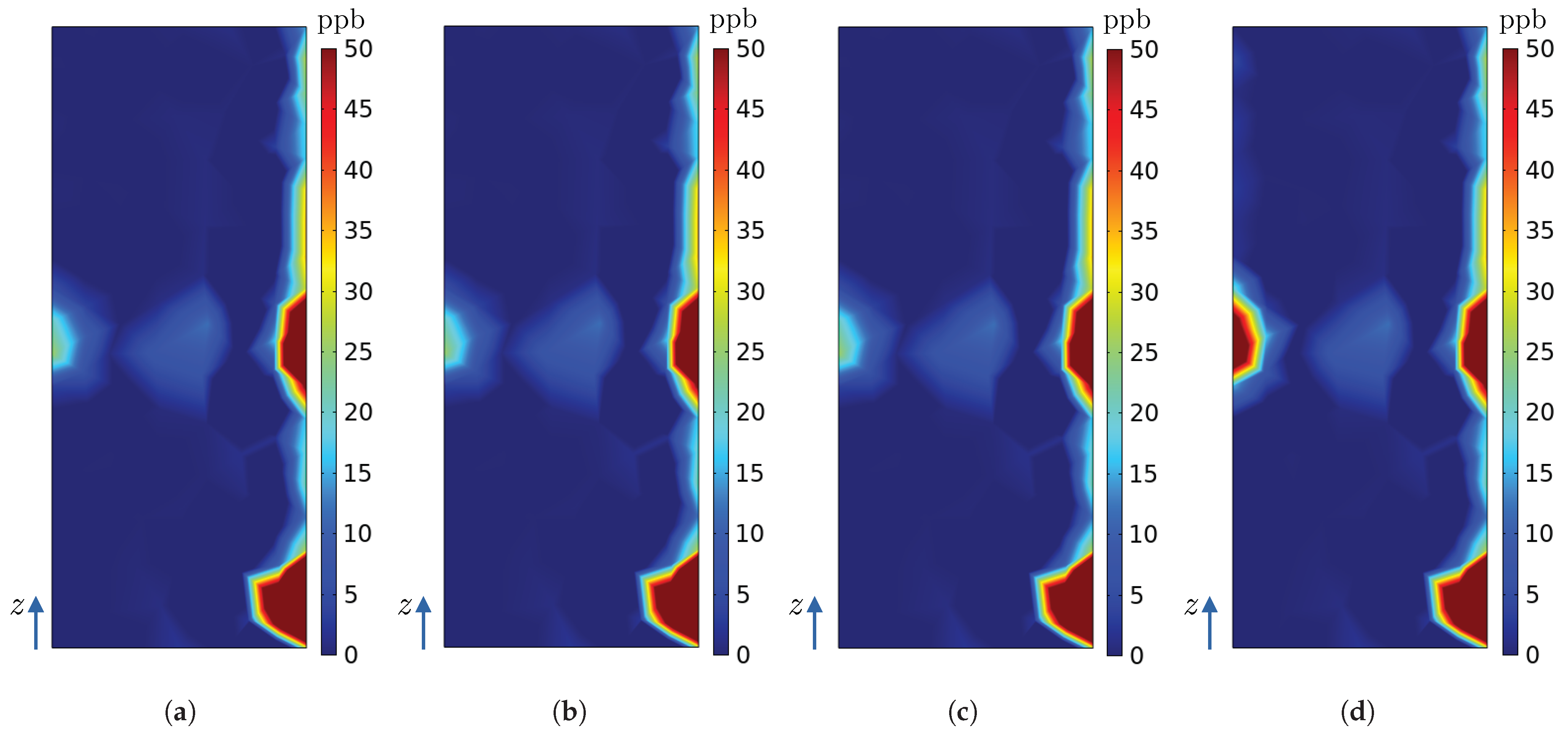
Figure 27.
Ozone concentration (ppb) on the surfaces of the radiators and in the numerical model of the hydrogenerator: (a) (simulation E), (b) (simulation F), (c) (simulation E), and (d) (simulation F).
Figure 27.
Ozone concentration (ppb) on the surfaces of the radiators and in the numerical model of the hydrogenerator: (a) (simulation E), (b) (simulation F), (c) (simulation E), and (d) (simulation F).
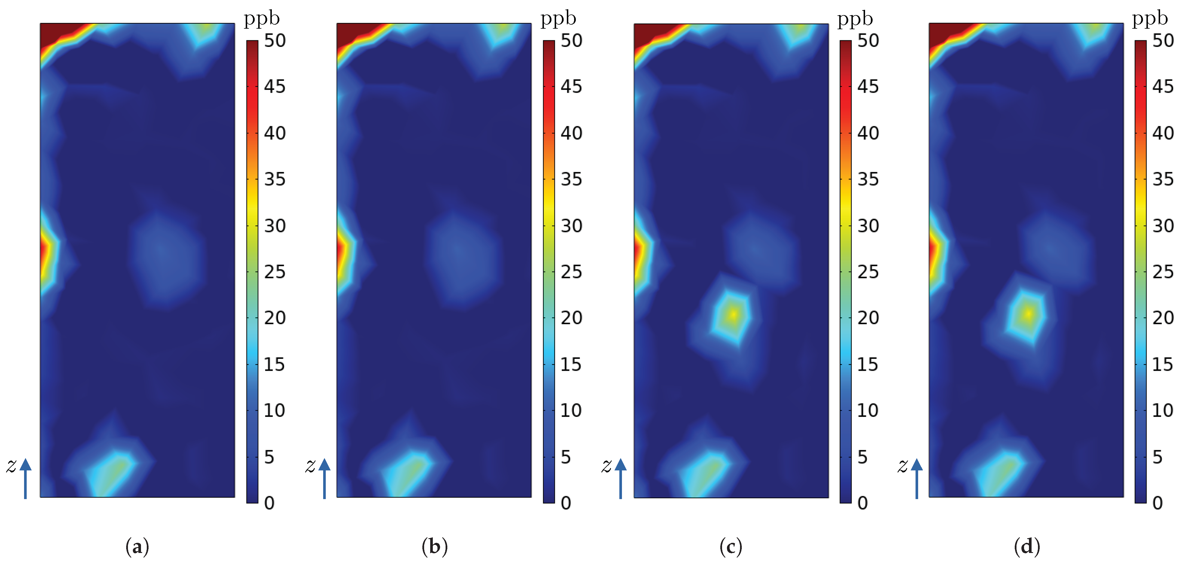
Figure 28.
Ozone concentration (ppb) on the surfaces of the radiators and in the numerical model of the hydrogenerator: (a) (simulation E), (b) (simulation F), (c) (simulation E), and (d) (simulation F).
Figure 28.
Ozone concentration (ppb) on the surfaces of the radiators and in the numerical model of the hydrogenerator: (a) (simulation E), (b) (simulation F), (c) (simulation E), and (d) (simulation F).
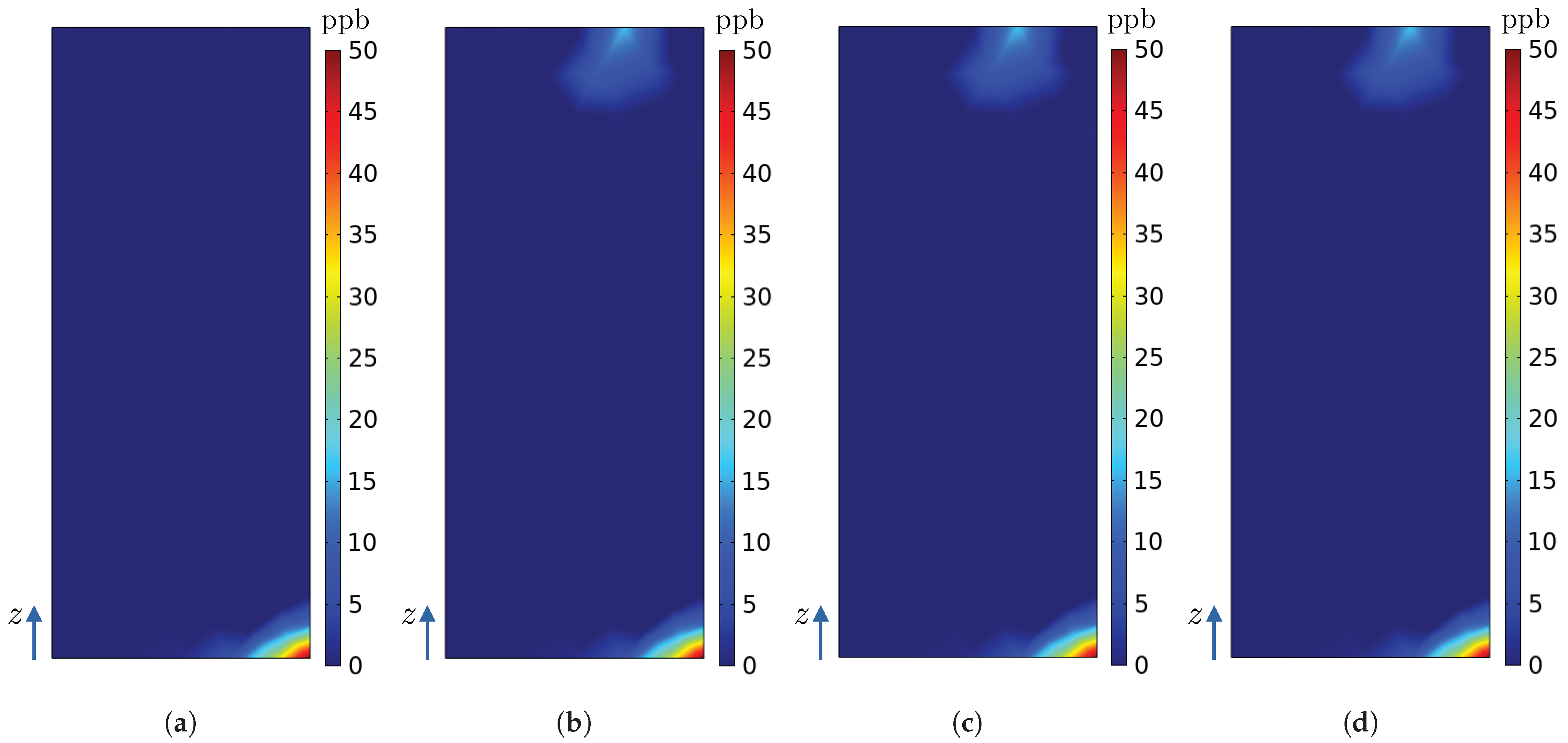
Figure 29.
Ozone concentration (ppb) on the surfaces of the radiators and in the numerical model of the hydrogenerator: (a) (simulation E), (b) (simulation F), (c) (simulation E), and (d) (simulation F).
Figure 29.
Ozone concentration (ppb) on the surfaces of the radiators and in the numerical model of the hydrogenerator: (a) (simulation E), (b) (simulation F), (c) (simulation E), and (d) (simulation F).
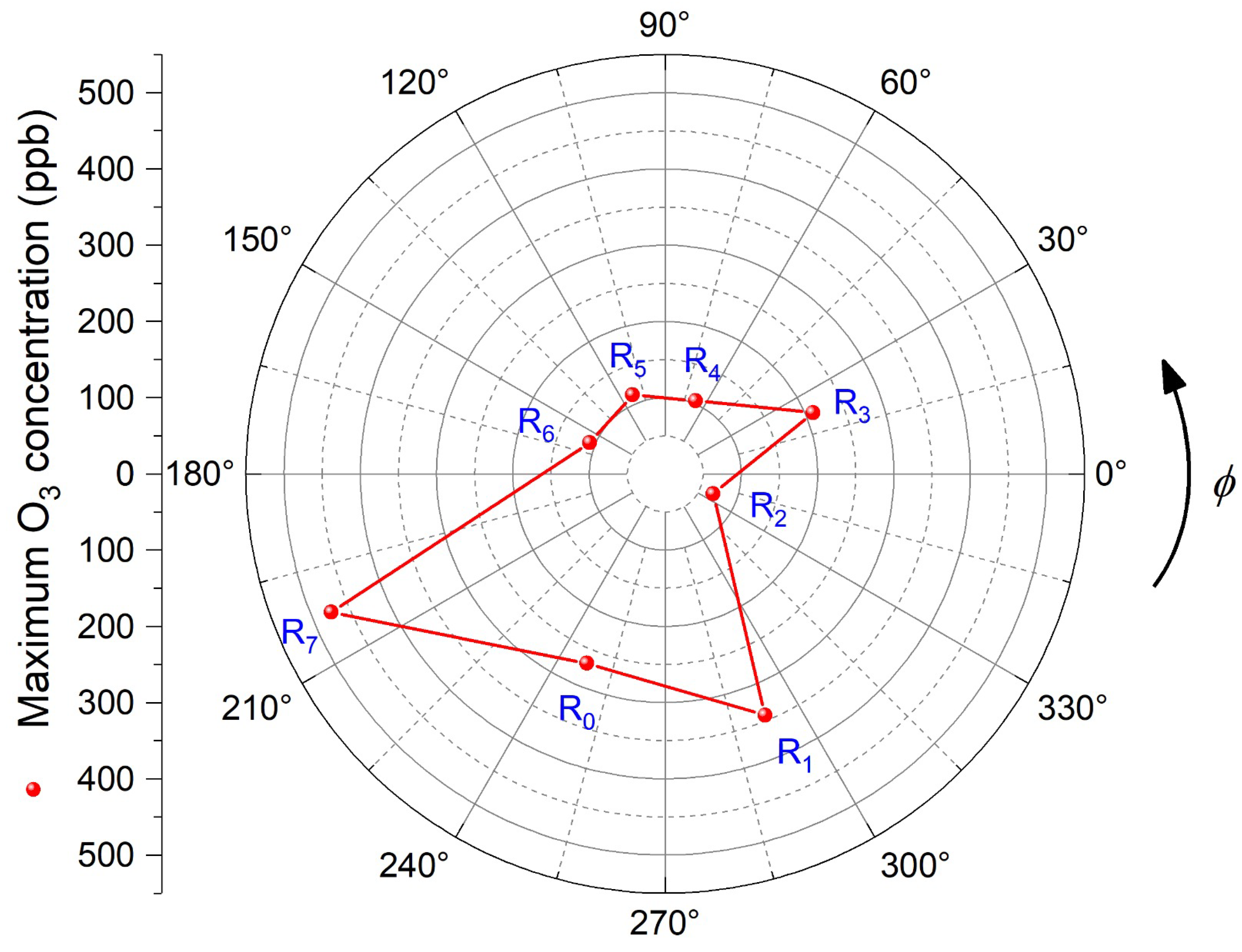
Figure 30.
Maximum concentrations of ozone on the radiators as a function of (numerical model).
Figure 30.
Maximum concentrations of ozone on the radiators as a function of (numerical model).
Table 1.
Values of adopted for different materials in our numerical model.
Table 1.
Values of adopted for different materials in our numerical model.
| Material | | Reference |
|---|
| Stainless steel | 1.8 × 10 | Mueller et al. [36] |
| Concrete | 7.9 × 10 | Simmons and Colbeck [37] |
| Semiconductor coating layer | 1.11 × 10 | Cataldo and Ursini [38] |
| Epoxy | 2.0 × 10 | Reiss et al. [39,40] |
| Copper | 5.5 × 10 | Gusakov et al. [41] |
Table 2.
The represented components and structural parts of the hydrogenerator, materials, and geometric details.
Table 2.
The represented components and structural parts of the hydrogenerator, materials, and geometric details.
| Components and Structural Parts | Material | Geometric Details |
|---|
| Floor and external walls | Concrete | Figure 2 |
| Rotor | Surface of epoxy | Figure 2 |
| 378 coil-type stator bars | Copper covered by mica and a semiconductor coating layer | Figure 3 |
| Stator core | Stainless steel | Figure 4 |
| Air directors | Stainless steel | Figure 5 |
| Radiator | Copper | Figure 5 |
Table 3.
Ozone source locations in simulations A to D: vertical and angular coordinates, height category, and sectors.
Table 3.
Ozone source locations in simulations A to D: vertical and angular coordinates, height category, and sectors.
| Source | Vertical Coordinate z (m) | Height Category | Angular Coordinate | Sector |
|---|
| 2.074 | intermediary | 270° | between and |
| 2.074 | intermediary | 280° | |
| 2.074 | intermediary | 292.5° | |
| 0.574 | bottom | 305° | |
| 2.074 | intermediary | 315° | between and |
| 3.574 | top | 315° | between and |
| 4.020 | top | 330° | |
| 0.574 | bottom | 330° | |
| 1.574 | intermediary | 340° | |
| 2.074 | intermediary | 350° | |
| 4.020 | top | 22.5° | |
| 0.272 | bottom | 0° | between and |
Table 4.
Volume and ozone average volumetric concentration for each source (simulations A to D).
Table 4.
Volume and ozone average volumetric concentration for each source (simulations A to D).
| Source | Dimensions (mm) | Volume (mm) | Ozone Average Volumetric Concentration (ppb) |
|---|
| 20.2×20×15 | 6060 | 22,000 |
| 20.2 × 15 × 10 | 3030 | 11,000 |
| 20.2 × 15 × 10 | 3030 | 11,000 |
| 47.2 × 25 × 15 | 17,700 | 64,257.43 |
| 30 × 20.2 × 15 | 9090 | 33,000 |
| 20.2 × 20 × 15 | 6060 | 22,000 |
| 15 × 15 × 15 | 3375 | 12,252.48 |
| 20.2 × 15 × 15 | 4545 | 16,500 |
| 20.2 × 20.2 × 15 | 6120.6 | 22,220 |
| 20.2 × 15 × 10 | 3030 | 11,000 |
| 15 × 15 × 15 | 3375 | 12,252.48 |
| 15×15×15 | 3375 | 12,252.48 |
Table 5.
Ozone concentrations (ppb) in personnel circulation corridor and on surface of radiators for each simulation (from A to B).
Table 5.
Ozone concentrations (ppb) in personnel circulation corridor and on surface of radiators for each simulation (from A to B).
| Concentration Parameter | Simulation A | Simulation B | Simulation C | Simulation D |
|---|
| Maximum concentration in personnel circulation corridor | 209.37 | 209.32 | 209.35 | 209.32 |
| Average concentration in personnel circulation corridor | 3.9630 | 3.9602 | 3.9515 | 4.3975 |
| Maximum concentration on radiator | 0 | 0 | 0 | 25 |
| Average concentration on radiator | 0 | 0 | 0 | 0.2431 |
| Maximum concentration on radiator | 159 | 159 | 159 | 159 |
| Average concentration on radiator | 3.7132 | 3.7122 | 3.7124 | 4.1252 |
| Maximum concentration on radiator | 209 | 209 | 209 | 209 |
| Average concentration on radiator | 2.47 | 2.4715 | 3.0153 | 3.0152 |
| Maximum concentration on radiator | 51.1 | 51.7 | 51.3 | 51.3 |
| Average concentration on radiator | 0.2605 | 0.49 | 0.4842 | 0.4842 |
| Maximum concentration on radiator | 7.61 | 7.62 | 7.54 | 7.54 |
| Average concentration on radiator | 0.0728 | 0.1169 | 0.1172 | 0.1172 |
Table 6.
Percentage differences between the maximum ozone concentrations among the simulations.
Table 6.
Percentage differences between the maximum ozone concentrations among the simulations.
| Region | | | | | | |
|---|
| Personnel circulation corridor | 0.0239 | 0.0095 | 0.0239 | 0.0143 | 0 | 0.0143 |
| Radiator | – | – | 100 | – | – | – |
| Radiator | 0 | 0 | 0 | 0 | 0 | 0 |
| Radiator | 0 | 0 | 0 | 0 | 0 | 0 |
| Radiator | 1.1742 | 0.3914 | 0.3899 | 0.7737 | 0.7737 | 0 |
| Radiator | 1.6 | 0.5333 | 0.5305 | 1.0499 | 1.0499 | 0 |
Table 7.
Percentage differences between the spatial average ozone concentrations among the simulations.
Table 7.
Percentage differences between the spatial average ozone concentrations among the simulations.
| Region | | | | | | |
|---|
| Personnel circulation corridor | 0.0706 | 0.2902 | 9.8806 | 0.2197 | 11.0424 | 11.2868 |
| Radiator | – | – | 100 | – | – | – |
| Radiator | 0.0269 | 0.02154 | 9.9874 | 0.0054 | 11.1255 | 11.1195 |
| Radiator | 0.0607 | 22.0769 | 18.0817 | 22.0028 | 21.9988 | 0.0033 |
| Radiator | 88.1517 | 85.9211 | 46.2093 | 1.1856 | 1.1937 | 0.0083 |
| Radiator | 60.4591 | 60.9258 | 37.8467 | 0.2909 | 0.2652 | 0.0256 |
Table 8.
Location of each ozone source in simulations E and F, their height class, and sector.
Table 8.
Location of each ozone source in simulations E and F, their height class, and sector.
| Source | Vertical Position z (m) | Height Class | Azimuth Position | Sector |
|---|
| 3.524 | top | 265° | |
| 3.624 | top | 270° | between and |
| 3.574 | top | 275° | |
| 3.674 | top | 280° | |
| 3.424 | top | 285° | |
| 2.074 | intermediary | 75° | |
| 1.574 | intermediary | 75° | |
| 0.674 | bottom | 310° | |
| 0.574 | bottom | 310° | |
Table 9.
Volume and ozone average volumetric concentration for each source in simulations E and F.
Table 9.
Volume and ozone average volumetric concentration for each source in simulations E and F.
| Source | Dimensions (mm) | Volume (mm) | Ozone Average Volumetric Concentration (ppb) |
|---|
| 20.2 × 15 × 15 | 4545 | 16,500 |
| 47.2 × 20 × 15 | 14,160 | 51,405.94 |
| 25 × 20.2 × 15 | 7575 | 27,500 |
| 47.2 × 20 × 15 | 14,160 | 51,405.94 |
| 47.2 × 20 × 15 | 14,160 | 51,405.94 |
| 60 × 20.2 × 10 | 12,120 | 44,000 |
| 30 × 20.2 × 10 | 6060 | 22,000 |
| 47.2 × 15 × 15 | 10,620 | 38,554.46 |
| 47.2 × 25 × 15 | 17,700 | 64,257.43 |
Table 10.
Maximum ozone concentration on each radiator.
Table 10.
Maximum ozone concentration on each radiator.
| Radiator | Angular Position (°) | Maximum Ozone Concentration (ppb) |
|---|
| 247.5° | 268.96 |
| 292.5° | 342.42 |
| 337.5° | 68.309 |
| 22.5° | 209.83 |
| 67.5° | 103.77 |
| 112.5° | 111.92 |
| 157.5° | 107.27 |
| 202.5° | 473.83 |


 ,
, 


