Supervised Contrastive Learning for Fault Diagnosis Based on Phase-Resolved Partial Discharge in Gas-Insulated Switchgear

Abstract

Supervised contrastive learning (SCL) has recently emerged as an alternative to conventional machine learning and deep neural networks. In this study, we propose an SCL model with data augmentation techniques using phase-resolved partial discharge (PRPD) in gas-insulated switchgear (GIS). To increase the fault data for training, we employ Gaussian noise adding, Gaussian noise scaling, random cropping, and phase shifting for supervised contrastive loss. The performance of the proposed SCL was verified by four types of faults in the GIS and on-site noise using an on-line ultra-high-frequency (UHF) partial discharge (PD) monitoring system. The experimental results show that the proposed SCL achieves a classification accuracy of 97.28% and outperforms the other algorithms, including support vector machines (SVM), multilayer perceptron (MLP), and convolution neural networks (CNNs) in terms of classification accuracy, by 6.8%, 4.28%, 2.04%, respectively.

1. Introduction

Power systems have advanced considerably, with electricity playing a crucial role in the manufacturing industry and our daily life. However, the use of high current carries the risk of fire, equipment explosions and damage to the system. To mitigate these risks, maintaining stability in system operations is important. Gas-insulated switchgear (GIS) is a type of electrical equipment that uses gas to insulate and protect different parts of power transmission and distribution systems [1]. GIS is advantageous because it has a small size [2] and flexible configuration and is easy to maintain [3].

In power systems, partial discharges (PDs) ensure the reliability and safety of the electrical infrastructure. When PDs occur in GIS, the insulation deterioration increases, thereby resulting in serious accidents owing to insulation defect. Hence, PD detection in the early phase is very important [4]. Different methods have been developed to detect PDs, including the use of loop antennas, acoustic emissions, or different types of internal and external sensors [5,6,7,8]. Among these methods, ultra-high-frequency (UHF) sensors can capture a wide range of frequencies and effectively reduce noise [9]. Therefore, we use PD signals from UHF sensors for fault diagnosis in GIS [10].

Recently, artificial intelligence (AI) has successfully performed pattern recognition and classification of PD in GIS using various machine learning algorithms, such as support vector machines (SVMs), random forests (RF), logistic regression (LR), k-nearest neighbors (kNNs) and backpropagation neural networks (BPNN) [11,12,13,14,15,16]. The classification of PD signals involves two distinct patterns: time-resolved partial discharges (TRPDs) and phase-resolved partial discharges (PRPDs). The TRPD-based methods for pattern recognition and classification have the advantage of a simple measurement system and the ability to distinguish signals from noise [11,12,13,16]. SVM with chromatic methodology is used for TRPD-based pattern recognition [11]. Also, based on TRPD, PD classification is proposed through RF with Hilbert transform [12], and incipient discharge classification is proposed through RF and kNN using FFT analysis  [13]. The PRPD-based methods for pattern recognition and classification method have robustness against signal attenuation and noise interference [14,15,16]. Based on PRPD, a PD severity assessment is proposed, utilizing a minimum-redundancy maximum-relevance algorithm-based feature selection and SVM [14]. A two-step LR is proposed for the identification of multisource PDs based on each PRPD pattern [15]. Moreover, partial discharge recognition is proposed using BPNNs and integrating information from both TRPD and PRPD [16]. The limitation in extracting high-level features are the big issues for conventional machine learning techniques [17]. This is because the feature extraction process in machine learning techniques is time-consuming and depends on domain expertise [17].

To address the disadvantages of machine learning techniques, deep neural networks (DNNs) have been developed, performing complex calculations with large amounts of data. The DNN-based PD classification method, which consists of multiple hidden layers and activation functions, was proposed using UHF PRPD [16]. However, the convergence of the structure is slow and complicated owing to numerous nonlinear activation functions, layers, and neurons. To solve the DNN problem, CNNs have been proposed in some studies, including PRPD pattern recognition of GIS [18], TRPD pattern recognition of GIS [19], and transfer learning combined CNN with the IoT for the automatic management of GIS [20]. CNNs comprise different convolution blocks and fully connected layers. Further, different types and variations of the CNN architectures have been proposed, including AlexNet, VGG, ResNet, and GoogLeNet [21]. While CNNs demonstrate remarkable learning capabilities than conventional machine learning methods, those employed for fault diagnosis require a large training dataset [22]. In the fault diagnosis for GIS, obtaining extensive fault data based on different environments and levels of failure severity is challenging.

In this study, we propose a novel approach for fault diagnosis in GIS by utilizing supervised contrastive learning (SCL) with PRPD signals. Our work builds upon recent successes in supervised learning. This is exemplified by proposing a supervised contrastive learning-based domain adaptation network (SCLDAN) for cross-domain fault diagnosis of the rolling bearing [23], using multimodal SCL to classify MRI regions for prostate cancer diagnosis [24], SCL for image dataset cleaning [25], and SCL for text representation [26] in related studies. Contrastive learning aims to maximize the similarity between any two vector representations by minimizing the contrastive loss function, and its advantage includes distinguishing different types of data [27]. The proposed SCL model comprises pretrained and downstream tasks. As regards the pretrained task, we propose new data augmentation methods for the PRPDs in GIS. For data augmentation, we employ Gaussian noise adding, Gaussian noise scaling, random cropping, and phase shifting to generate more views as input for supervised contrastive loss. To validate the robustness and effectiveness of the proposed SCL model, we conduct experiments using PRPDs and on-site noises in GIS. The proposed SCL achieves a classification accuracy of 97.28%, thereby outperforming conventional methods such as SVM, MLP, and CNN in terms of classification performance with margins of 6.8%, 4.28%, and 2.04%, respectively.

The remainder of this paper is organized as follows: In Section 2, works related to the SCL method and measurement of PRPDs in GIS are presented. The proposed SCL model, including data augmentation, is presented in Section 3. The validation results based on measured PRPDs and noise are presented in Section 4. Section 5 concludes this paper.

2. Related Works

In this section, we introduce the SCL and present our experimental setup and measurement results for the PRPDs using UHF sensors to evaluate the PD characteristics of the GIS system.

2.1. Supervised Contrastive Learning

The SCL learns representations that capture information shared between multiple sensory views without human supervision [27,28]. The SCL is divided into pretrained and downstream tasks.

2.1.1. Pretrained Task

Figure 1 shows the pretrained task for the SCL model, in which the input data are augmented to create two new versions with different views using data augmentation techniques, which will be explained in Section 3. After data augmentation, the encoder takes the different data views and represents them into embedding space with high-level features. In the pretrained task, the weights of the encoder are preserved and frozen to serve for the downstream task. The projection head uses a series of nonlinear layers to apply nonlinear transformations and project the obtained encoder. The pretrained task aims to minimize the value of the contrastive loss function, which evaluates the similarity between any two inputs.

2.1.2. Contrastive Loss

The contrastive loss of SCL receives each augmented pair in the minibatch of the encoder to compare and provide the similarity. The clusters of points belonging to the same class are pulled together in embedding space, while simultaneously pushing apart clusters of samples from different classes [27]. Hence, the amount of information gained from labeled data will be exploited more effectively than the cross-entropy loss. The contrastive loss function is defined as [27]

$$L^{sup}=\sum _{i\in I}{L}_i^{sup}=\sum _{i\in I}\frac{-1}{\left|P\right(i\left)\right|}\sum _{p\in P\left(i\right)}log\frac{exp({\mathit{z}}_i·{\mathit{z}}_p/\tau )}{{\sum }_{a\in A\left(i\right)}exp({\mathit{z}}_i·{\mathit{z}}_a/\tau )}.$$

(1)

A detailed explanation of the formula in (1) is provided in Section 3.2. Here, the contrastive loss function is more robust and less sensitive to the changes in the hyperparameters.

2.1.3. Downstream Task

After obtaining the frozen encoder from the pretrained task, a downstream task fine-tunes it to not only achieve the goal of the given problem, but also to yield better performance for the underlying task. The downstream task transfers what is learned from the pretrained tasks for classification, detection, and segmentation [29]. In this study, the downstream task is PRPD classification for fault diagnosis in GIS.

2.2. PRPD Measurements and On-Site Noise for GIS

Here, we present PD measurements and on-site noise using artificial cells and the on-line UHF PD monitoring system, respectively, for GISs.

Figure 2 shows a block diagram comprising a GIS, an external UHF sensor, and a data acquisition system (DAS) for PD and noise measurements. The UHF sensor for measuring PD signals has a frequency range of 0.5 to 1.5 GHz, and a sensitivity level of −14.5 dBm at 5 pC, which is verified based on CIGRE TF 15/33.03.05 [30]. In the measurement system, artificial cells for PD modeling and an external UHF sensor were installed in a 345 kV GIS chamber. To simulate possible defects in a GIS, we used artificial cells that model four types of defects (corona, suspended, particle, and void PD) [31]. The DAS utilized a peak detector to capture the maximum values of the UHF sensor for the PRPD signals.

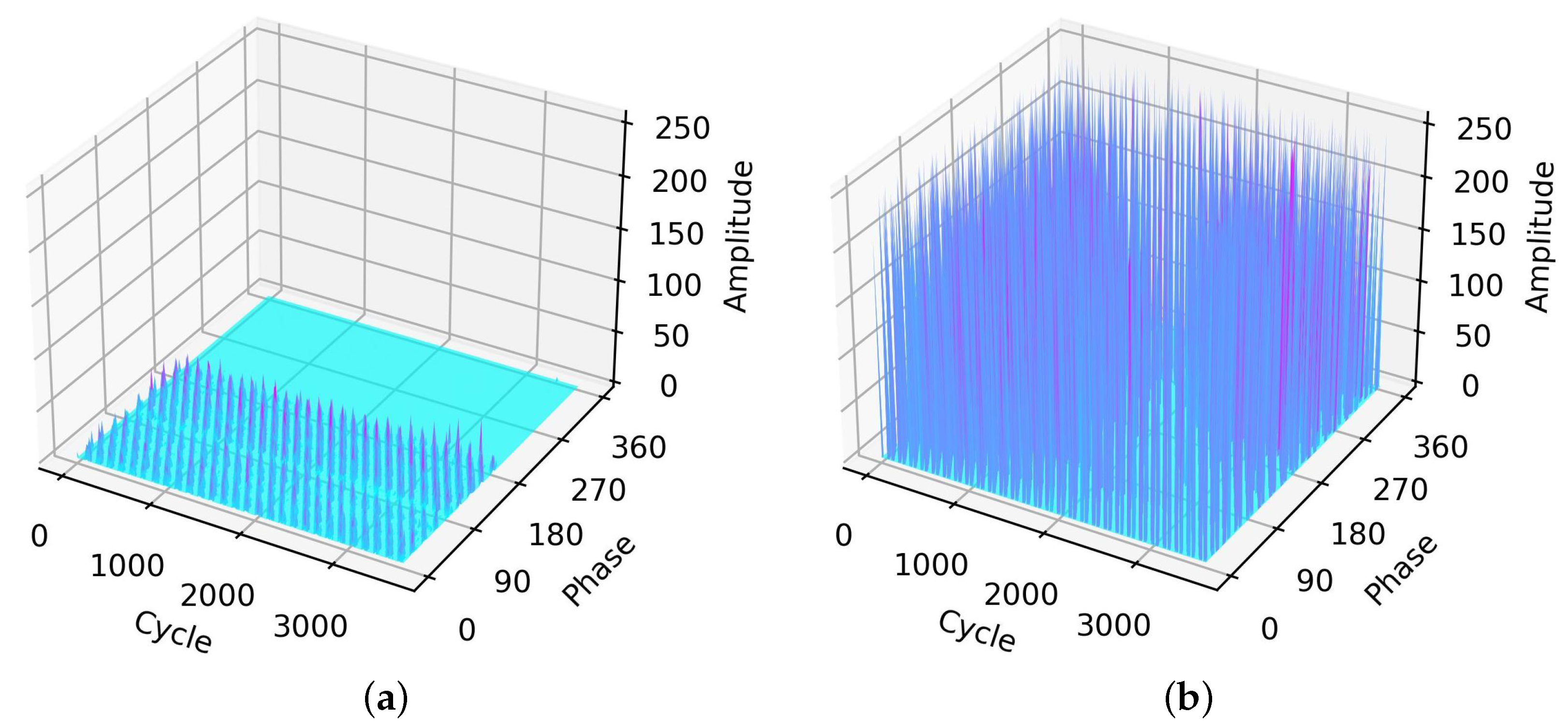
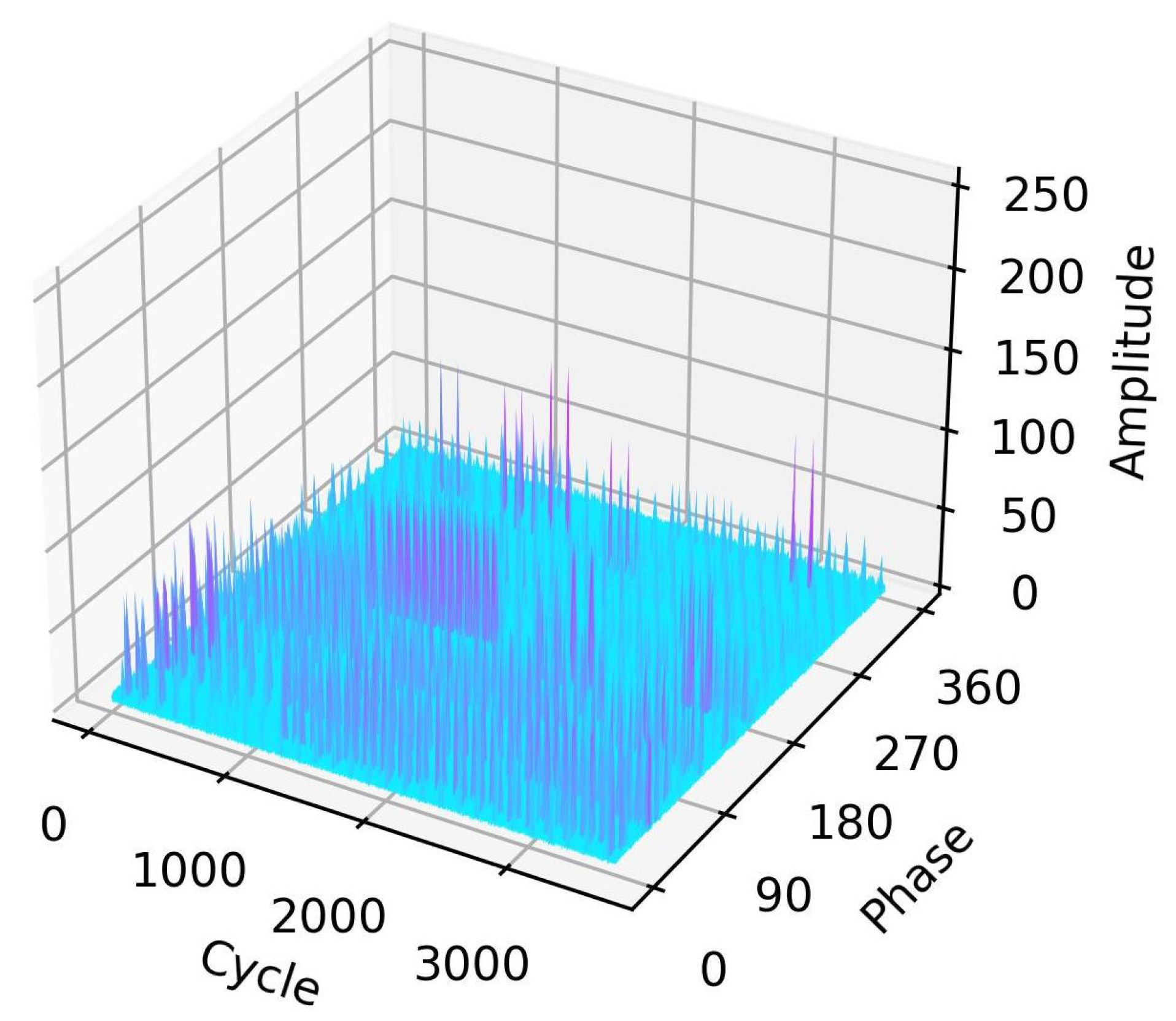
2.2.1. PRPD Measurements

The PRPD signal at the mth power cycle is defined as ${\mathit{x}}_m=[x_{m1},x_{m2},\cdots ,x_{mN}]$, where $m=1,2,\cdots ,M$: M is the number of power cycles, and N is the number of phase angles in a power cycle. In the matrix form, the PRPD signal is expressed as

$$\mathit{X}={[{\mathit{x}}_1^T,{\mathit{x}}_2^T,\cdots ,{\mathit{x}}_M^T]}^T,$$

(2)

where X is the N × M matrix.

Figure 3 presents data for the PRPDs under the four types of faults with 3600 power cycles using a UHF sensor ($M=3600$). As shown in Figure 3b, the floating discharge pulses are widely distributed throughout the graph with a very high intensity, reaching approximately the threshold of 250. A similar trend occurs in the particle; however, the intensity is unstable and lower (the average is approximately 150) compared to the floating. From the aforementioned, both types of discharge pulses (including corona and void) have an almost similar type of distribution when concentrating more on the under half. As regards corona and void, the pulses are distributed from 0${}^{\circ }$ to approximately 200${}^{\circ }$ and 0${}^{\circ }$ to approximately 240${}^{\circ }$, respectively.

2.2.2. On-Site Noise

On-site noise measurements were conducted using an online UHF PD monitoring system. As shown in Figure 4, pulses exhibit relatively low amplitudes and are concentrated throughout the phases.

Figure 5 shows the t-distributed stochastic neighbor embedding (t-SNE) for the input vectors of five PD defect types, where t-SNE creates a lower-dimensional map that presents the intrinsic structures in a high-dimensional dataset through a nonlinear dimension reduction technique [32]. Although the t-SNE converts vectors with high-dimension into 2D space, it still keeps the local similarities and provides a visual indication of the data arrangement from initial vectors [33]. As shown in Figure 5, the distributions of the raw UHF signals are mixed with the high density, thereby making it impossible to distinguish discharge defects only by seeing the input t-SNE graph without performing any transformation.

3. Proposed Scheme

In this section, we propose the SCL model for the PRPD classification in a GIS. The proposed SCL model comprises pretrained and downstream tasks. In the pretrained task, data augmentation is performed, and the augmented data are passed through the encoder network first to create the frozen-weight encoder before being fed into the projection head. After contrastive loss minimization, the frozen-weight encoder is used for the downstream task. A classifier for PRPD classification is applied as the downstream task.

3.1. Data Augmentation

In the proposed SCL model, we propose four augmentation techniques, namely Gaussian noise adding, Gaussian noise scaling, random cropping, and phase shifting. Data augmentation is performed to increase the number of training data for fault diagnosis [34].

3.1.1. Gaussian Noise Adding

Gaussian noise adding is expressed as

$${\tilde{x}}_{ij}^{GA}=x_{ij}+n_1,$$

(3)

where $n_1$ is a Gaussian distribution with $N({\mu }_1,{\sigma }_1^2)$, $x_{ij}$ is the component of the PRPD matrix X in (1), and ${\tilde{x}}_{ij}^{GA}$ is the component of the matrix ${\tilde{\mathbf{X}}}^{GA}$. The Gaussian noise adding ${\tilde{\mathbf{X}}}^{GA}=GA\left(\mathbf{X}\right)$ considers different noise environments.

3.1.2. Gaussian Noise Scaling

Gaussian noise scaling is expressed as

$${\tilde{x}}_{ij}^{GS}=n_2\ast x_{ij},$$

(4)

where $n_2$ is a Gaussian distribution with $N({\mu }_2,{\sigma }_2^2)$. The Gaussian noise scaling ${\tilde{\mathbf{X}}}^{GS}=GS\left(\mathbf{X}\right)$ considers changes in the amplitude of PDs depending on the severity of the faults, in which the $(i,j)$-entry of a matrix ${\tilde{\mathbf{X}}}^{GS}$ is ${\tilde{x}}_{ij}^{GS}$ as expressed in (4).

3.1.3. Random Cropping

Random cropping is expressed as

$${\tilde{\mathbf{X}}}^{RC}=RC\left(\mathbf{X}\right),$$

(5)

where $RC(·)$ changes $c\%$ of the components of the input matrix to 0. Based on the severity of the faults, the random cropping considers changes in the amplitude of the PDs.

3.1.4. Phase Shifting

Phase shifting is expressed as

$${\tilde{\mathbf{X}}}^{PS}=PS\left(\mathbf{X}\right),$$

(6)

where $PS(·)$ permutes phases of the input matrix. This modification considers the phase synchronization errors between the electrical equipment and fault diagnosis system.

After the data augmentation, $\tilde{\mathbf{X}}$ is constructed by selecting two of the four matrices, $\{{\tilde{\mathbf{X}}}^{GA},{\tilde{\mathbf{X}}}^{GS},{\tilde{\mathbf{X}}}^{RC},{\tilde{\mathbf{X}}}^{PS}\}$. For a set of T randomly sampled sample/label pairs, ${\{{\mathbf{X}}_t,y_t\}}_{t=1,\cdots ,T}$, the corresponding batch used for training comprises $2T$ pairs, ${\{{\tilde{\mathbf{X}}}_i,{\tilde{y}}_i\}}_{i=1,\cdots ,2T}$, where ${\tilde{\mathbf{X}}}_{2t}$ and ${\tilde{\mathbf{X}}}_{2t-1}$ are two random augmentations of ${\mathbf{X}}_t$ ($t=1,\cdots ,T$) and ${\tilde{y}}_{2t-1}={\tilde{y}}_{2t}=y_t$.

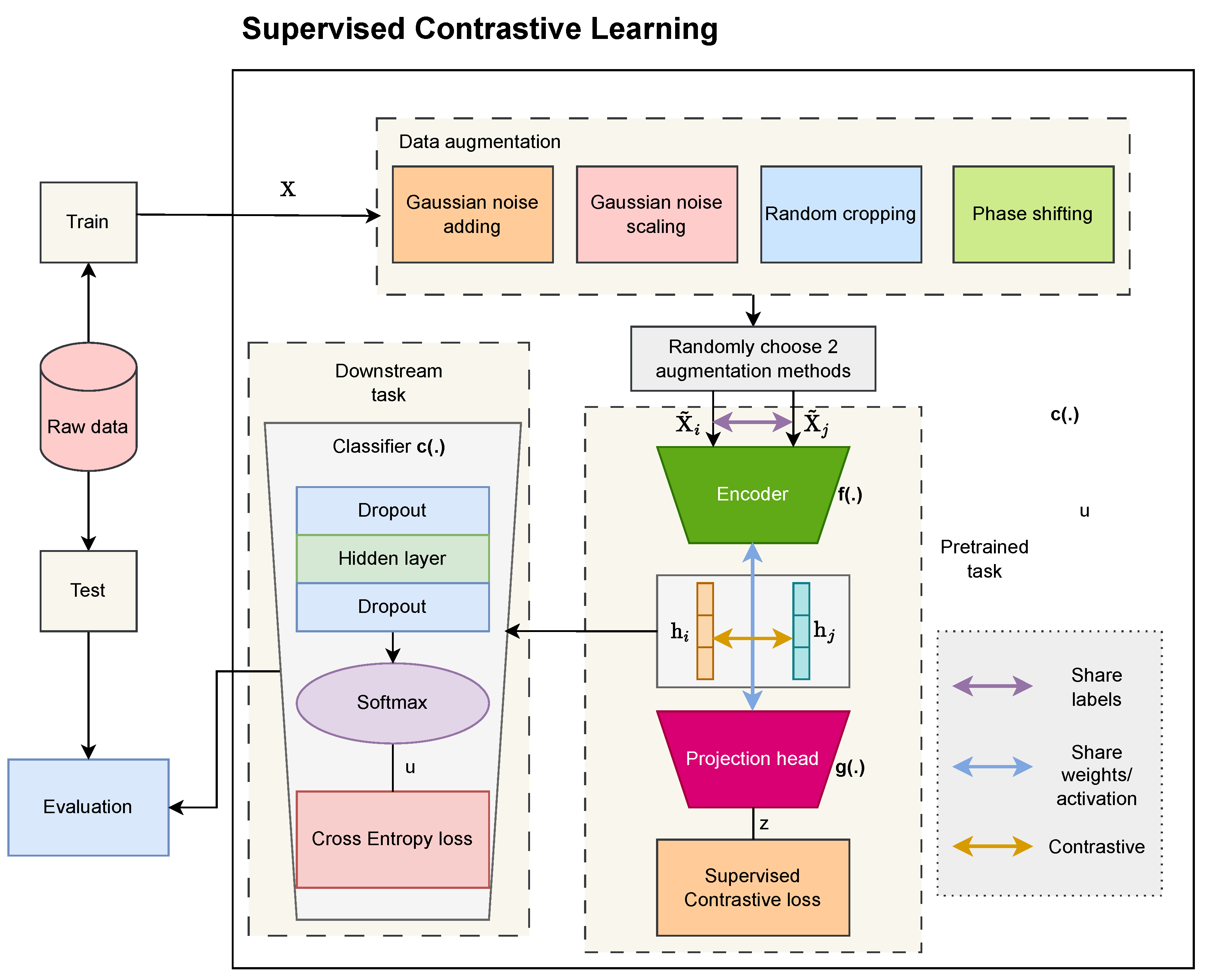
3.2. Supervised Contrastive Learning

Figure 6 shows a block diagram of the proposed SCL model. The pretrained and downstream tasks are performed after data augmentation.

The pretrained task comprises an encoder network, a projection head, and a supervised contrastive loss. It is described as follows.

1.

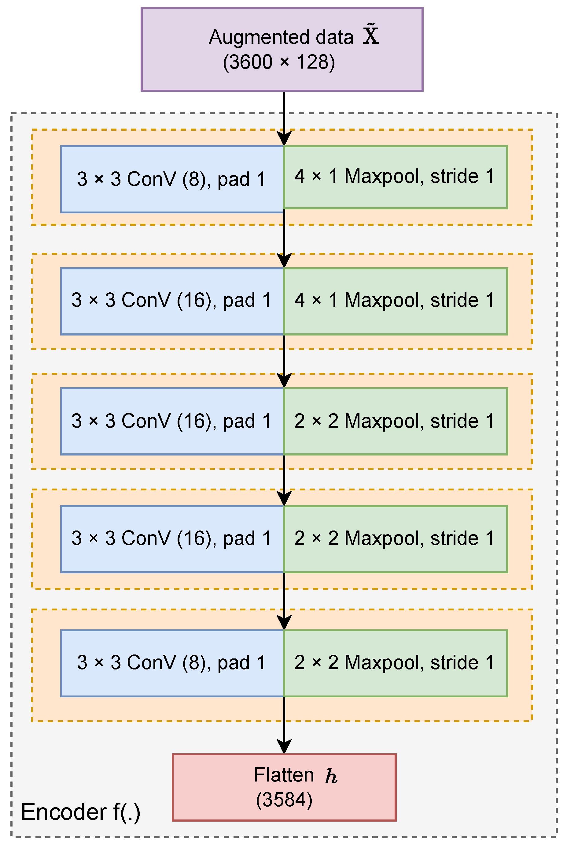
The first part is encoder network $f(·)$ with the operation to turn the two-dimensional matrix $\tilde{\mathbf{X}}$ into a one-dimensional vector, which is denoted as $\mathit{h}=f\left(\tilde{\mathbf{X}}\right)\in R^{D_f}$, where $D_f$ is the output shape of the last layer in the network. From ${\tilde{\mathbf{X}}}_{2t-1}$ and ${\tilde{\mathbf{X}}}_{2t}$, we obtain a pair of representation vectors ${\mathit{h}}_{2t-1}$ and ${\mathit{h}}_{2t}$, respectively. The encoder network comprises convolution layers to extract high features and a flattened layer.

2.

Projection head $g(·)$ is expressed as ${\mathit{z}}_i=g\left({\mathit{h}}_i\right)\in R^{D_g}$, where $g(·)$ comprises a single linear layer of $D_g$ units with a nonlinear activation ReLU function and $i\in I\equiv 1,\cdots ,2T$ is the index of an arbitrary augmented sample within a multiviewer batch.

3.

The supervised contrastive loss is expressed as [24]

$$L^{sup}=\sum _{i\in I}{L}_i^{sup},$$

(7)

with

$$\begin{array}{c}\hfill \begin{array}{c}{L}_i^{sup}=\frac{-1}{\left|P\right(i\left)\right|}\sum _{p\in P\left(i\right)}log\frac{exp({\mathit{z}}_i·{\mathit{z}}_p/\tau )}{{\sum }_{a\in A\left(i\right)}exp({\mathit{z}}_i·{\mathit{z}}_a/\tau )},\end{array}\end{array}$$

(8)

where $A\left(i\right)\equiv I\setminus \left\{i\right\}$ is the set that eliminates element i from I and $P\left(i\right)\equiv \{p\in A\left(i\right)|{\tilde{y}}_p={\tilde{y}}_i\}$ is the set of indices of the positive samples whose label is the same as the i-th label. Here, $\tau$ > 0 denotes the scalar temperature parameter and $|·|$ denotes the total number of elements of the set.

4.

The target of the pretrained task is to minimize the contrastive loss function in (7). Consequently, the weights of the encoder $f(·)$ are frozen for the downstream task.

The downstream task uses the pretrained encoder $f(·)$ with the frozen weights before classification into $D_c$ classes. Classifier network $c(·)$ is expressed as $\mathit{u}=c\left(\mathit{h}\right)\in R^{D_c}$, where $c(·)$ comprises a hidden layer, two dropout layers, and a Softmax [35]. There are two 20%-dropout layers before and after the hidden layer to avoid overfitting. The cross-entropy loss function for the classifier network is expressed as

$$Loss\left(b\right)=-\sum _{j=1}^{D_c}{t}_{j}log\left(u_j^{\left(b\right)}\right),$$

(9)

where b is the index of the mini-batch, $t_j$ = 1 when the index j is the index for the ground truth, and $t_j$ = 0 in the other cases.

In our study, the raw dataset is divided into training and test sets. The Adam optimizer is used to update the learnable parameters for the supervised contrastive and cross-entropy loss functions [36]. The test set is used for evaluating the effectiveness of the proposed SCL. The overall training process of the proposed SCL is described in Algorithm 1.

Algorithm 1: Training process for the proposed SCL method

Input: training set X, label y, batch size B, temperature $\tau$, learning rate $\alpha$, and number of epochs E Data augmentation: $\tilde{\mathbf{X}}=$ randomly choose two augmented views from $\left\{GA\left(\mathbf{X}\right),GS\left(\mathbf{X}\right),RC\left(\mathbf{X}\right),PS\left(\mathbf{X}\right)\right\}$ Pretrained task:   1: for $n=1:E$ do   2:       for each minibatch $b\in B$ do   3:             for all $i\in b$ do   4:                    Encoder Network: ${\mathit{h}}_i\leftarrow f_{w_f}\left({\tilde{\mathbf{X}}}_i\right)$,   5:                    Projection Head: ${\mathit{z}}_i\leftarrow g_{w_g}\left({\mathit{h}}_i\right)$   6:               end for   7:                $L_i^{sup}$ for each i   8:         end for   9:         Supervised contrastive loss function all: 10:         $L^{sup}={\sum }_{i\in I}{L}_i^{sup}$ 11:         Update $w_f$, $w_g$ to minimize $L^{sup}$ in (6) 12: end for 13: return Encoder Network $w_f$. Downstream task:   1: Load frozen $w_f$ from Encoder Network   2: for $n=1:E$ do   3:       for each minibatch $b\in B$ do   4:             for all $i\in b$ do   5:                   ${\mathit{h}}_i\leftarrow f_{w_f}\left({\tilde{\mathbf{X}}}_i\right)$   6:                   Classifier Network: ${\mathit{u}}_i\leftarrow c_{w_c}\left({\mathit{h}}_i\right)$   7:              end for   8:              Cross-entropy loss function:   9:              $Loss\left(b\right)=-{\sum }_{j=1}^C{t}_{j}log\left(u_j^{\left(b\right)}\right)$ 10:       end for 11:       Update $w_c$ to minimize cross-entropy loss 12: end for 13: return Training, Validation accuracy Output: the proposed SCL model

4. Experimental Results

In this section, we present the performance evaluation of the fault diagnosis in power equipment using the proposed SCL.

Table 1. Experimental datasets for PRPDs.

Fault Type	Corona	Floating	Void	Particle	Noise	Overall
Number of experiments	94	35	242	66	298	735

shows the fault types (corona, floating, void, particle, and noise) and the number of measurement samples. A detailed description of the experimental signals is provided in Section 2.2.

For data augmentation, we choose the mean ${\mu }_1=0$ and standard deviation ${\sigma }_1=0.01$ as the parameters for Gaussian noise adding, ${\mu }_2$ = 1 and standard deviation ${\sigma }_2=0.01$ for Gaussian noise scaling, and $a=10$ for random cropping.

Figure 7 shows the structure of the encoder network, which comprises five convolutional blocks (each including a 3 × 3 convolution layer, a rectified linear unit activation and a max pooling layer) and a flatten layer with $D_f=3584$. After the encoder network, the projection head comprising a single hidden layer with $D_g=256$ and $\tau =0.05$ is used to apply nonlinear transformation and project $\mathit{h}$ to optimize the supervised contrastive loss in (6).

Regarding the downstream task, the classifier network comprises a 900-node hidden layer and a Softmax layer with $D_c=5$ for classifying five fault types.

In our experiment, the dataset was divided into training and testing sets with 80% and 20% sample proportions, respectively. In addition, data augmentation methods double the training set size. During training, we conducted experiments using different options to acquire optimized hyperparameters related to the batch size, number of layers, and filter size to optimize our method.

Table 2. Minimum and maximum bound for hyperparameter optimization for CNN and the proposed SCL.

Hyperparameter	Minimum	Maximum	Type
Minibatch size	8	128	Integer
Number of layers	1	8	Integer
Kernel size	3 × 3	7 × 7	Integer
Epochs	50	200	Integer
Learning rate	0.0001	0.01	Real
Classifier network nodes	600	1200	Integer
Projection head nodes	64	512	Integer
Dropout rate	0.2	0.5	Real

shows the optimization of the minimum and maximum bound for each hyperparameter, and their type as well. The proposed SCL was optimized using different combinations of parameters to obtain the best choice. After trying several architectures, we used the five convolution layers with a 3 × 3-size kernel for the encoder network, a single hidden layer with 256 nodes for the projection head and a 900-node hidden layer together with a 20% dropout rate for the classifier network. The combination of these architectures with the learning rate, batch size, and epochs of 0.0001, 16, and 200, respectively, achieves the highest overall classification accuracy for each fault type. In addition, we used the ReLU function to apply the nonlinear transformation for the SCL method with each combination of parameters. The programming language (Python) with Tensorflow version 2.12.0 and scikit-learn version 1.2.2 were used to process the fault diagnosis problem.

In this experiment, we compared the performance of the proposed SCL to the SVM with the nonlinear radial basis function (RBF) kernel, MLP, and CNN, where MLP uses ReLU activation and Adam optimizer with a maximum of 200 iterations. For SVM and MLP, we use feature extraction to reduce the two-dimensional raw data into one-dimensional vectors. The mean of the nonzero values and the number of nonzero values in each phase are used for feature extraction.

Table 3. Minimum and maximum bound for hyperparameter optimization for the SVM and MLP.

Hyperparameter	Minimum	Maximum	Type
SVM parameter	0.001	100	Real
Number of MLP hidden layers	1	5	Integer

shows the experiments for the SVM and MLP with various hyperparameter ranges. The regularization parameter $C_{SVM}$ for SVM has a range from 0.001 to 100 to avoid the overfitting problem, and the SVM model with $C_{SVM}=100$ reached the highest accuracy. For the MLP method, different numbers of hidden layers are tried from 1 to 5, and the number of nodes in each layer is reduced to prevent overfitting. After trying many sets with different numbers of nodes and hidden layers, we found the MLP model with (200, 150, 100, 50) nodes for four hidden layers with the highest accuracy. Here, we used the same range of hyperparameters and architectures for both the SCL encoder-classifier network and the CNN method as shown in Table 2. For the CNN model, the five convolution layers with a 3 × 3-size kernel, a 900-node hidden layer, and two-20% dropout layers with the learning rate, batch size, and epochs of 0.0001, 16, and 200, respectively, achieved the highest classification accuracy.

Table 4. Comparison of classification performance.

Fault Types	SVM (%)	MLP (%)	CNN (%)	Proposed SCL (%)
Corona	94.74	94.74	100	94.74
Floating	85.71	85.71	85.71	85.71
Particle	53.85	92.31	84.62	100
Void	87.50	91.67	95.83	95.83
Noise	100	93.33	96.67	100
Overall	90.48	93.00	95.24	97.28

presents the performance analysis for the proposed SCL. The proposed SCL is superior to the SVM owing to the difference in particle fault performance (100% in testing contrary to 53.85%). The proposed SCL outperforms the MLP by a margin of 4.28% in terms of the overall classification performance, with a particularly high performance in terms of classifying the particle, void, and noise. While the accuracy of the corona class in the proposed SCL is lower than that of the CNN, the overall performance (97.28% for the proposed SCL contrary to 95.24% for the CNN) remains superior, primarily owing to distinctions in particle and noise classifications. Hence, Table 4 shows that, in terms of accuracy, the proposed SCL is the best among the four methods.

For performance evaluation of imbalanced data set, $Precision$, $Recall$, and $F1\text{-}score$ are used [37]. $Precision$ and $Recall$ are defined as

$$Precision=\frac{TP}{TP+FP},$$

(10)

and

$$Recall=\frac{TP}{TP+FN},$$

(11)

respectively, where $TP$ is the number of accurately predicted samples as “positive”, $FP$ is the number of samples wrongly predicted as “positive”, and $FN$ represents the samples wrongly predicted as “negative”. $Precision$ represents the quality of a positive prediction made by the model, while $Recall$ is the fraction of positives that are correctly classified. $F1\text{-}score$ is the trade-off between $Precision$ and $Recall$, and is expressed as

$$F1\text{-}score=\frac{2}{\frac{1}{Precision}+\frac{1}{Recall}}=\frac{TP}{TP+\frac{1}{2}(FP+FN))}.$$

(12)

The range of the $F1\text{-}score$ is between 0 and 1, and the closer the value is to 1, the better the model. Conversely, the closer it is to 0, the worse the model.

Table 5. $Precision$, $Recall$, and $F1\text{-}score$ comparisons.

	Fault Types	Corona	Floating	Particle	Void	Noise
$Precision$	SVM	1	1	1	0.955	0.833
	MLP	1	0.750	0.857	0.957	0.918
	CNN	0.950	0.857	1	1	0.921
	Proposed SCL	1	1	0.929	0.979	0.968
$Recall$	SVM	0.947	0.857	0.538	0.875	1
	MLP	0.947	0.857	0.923	0.917	0.933
	CNN	1	0.857	0.846	0.958	0.967
	Proposed SCL	0.947	0.857	1	0.958	1
$F1-score$	SVM	0.973	0.923	0.700	0.913	0.909
	MLP	0.973	0.800	0.889	0.936	0.926
	CNN	0.974	0.857	0.917	0.979	0.943
	Proposed SCL	0.973	0.923	0.963	0.968	0.984

presents the $Precision$, $Recall$, and $F1\text{-}score$ for all classes between SVM, MLP, CNN, and the proposed SCL. The proposed SCL exhibits a notable performance in terms of $Precision$ and $Recall$, particularly in the noise class, where it achieves values of 0.968 and 1. Hence, the $F1\text{-}score$ reaches its peak at 0.984, surpassing other methods. The proposed SCL achieves a $Precision$ value of 1 in floating fault and a $Recall$ value of 1 in particle fault. The proposed SCL method achieves the highest $F1\text{-}score$s in three out of the five classes, excluding void and corona. This deviation is attributed to their lower $Recall$ values compared to the CNN (0.958 and 0.947 compared to 0.958 and 1, respectively), thereby resulting in a drop in the $F1\text{-}score$s for void and corona to the second place (0.963 and 0.973 for the proposed SCL compared to 0.917 and 0.974 for the CNN, respectively). In terms of $F1\text{-}score$ performance, the proposed SCL is better than SVM, MLP, and CNN, as presented in Table 5.

Figure 8 shows the confusion matrices for SVM, MLP, CNN, and the proposed SCL. It can be seen that both the proposed SCL and CNN only have two void samples that are misclassified as noise, while these metrics for the SVM and MLP are higher with the six and four misclassified void samples, respectively. In addition, the proposed SCL appears to be better than the other three methods in testing particle fault. As shown in Figure 8, the performance of the proposed SCL method is the best among four methods, with only a limited amount of the test data mistakenly recognized under other classes (one sample in the corona is misclassified as a void pattern, one sample in floating is misclassified as a particle, and two samples in void are misclassified as noise).

Table 6. Performance comparison of baseline CNNs using raw data and data augmentations.

Methods	Raw Data	GA	GS	RC	PS
Test Accuracy (%)	91.84	93.20	93.20	93.20	93.20

shows accuracies of the baseline CNN in the same condition for the data augmentation, where training data for the data augmentation technique consist of raw data and augmented data. It can be seen that when training raw data combined with the proposed data augmentation methods, the accuracy for the test set is better than only using the raw data. Figure 9 shows the confusion matrix in detail. All augmentation methods have an advantage in classifying noise class, while training only raw data leads to the five misclassified noise samples as four other faults.

Table 7. Training time and testing time comparisons.

Tasks	SVM	MLP	CNN	Proposed SCL
Training Time (s)	3.193	4.654	318.146	1154.029
Testing Time (s)	0.010	0.004	0.763	0.978

shows the training and testing times for SVM, MLP, CNN, and the proposed SCL. In our experiments, the models were trained and tested on a PC with an NVIDIA GeForce RTX 2080 Ti GPU and 128 Gb RAM. It can be seen that the training and testing times of the proposed SCL model were slower than those of SVM, MLP, and CNN. This was because the proposed SCL required data augmentation, the pretrained task, and the downstream task for the training. The test time of the proposed SCL took longer than that of other methods, but the duration was only 0.978 s, which is the computation complexity usable in a fault diagnosis system.

5. Conclusions

In this study, we proposed a SCL method to classify PRPDs in GISs. The proposed SCL model utilizes data augmentations for PRPDs and contrastive loss and cross-entropy loss functions. The advantages of the proposed SCL include distinguishing different PRPDs in GISs and evaluating the similarities between them using contrastive loss, while the different views of the training dataset are provided using different data augmentation methods. It was verified based on the PRPDs from artificial cells and on-site noise using an online UHF PD monitoring system for GISs. The PRPDs included four types of faults, namely corona, floating, particle, and void. The experimental results show that the proposed SCL achieved a classification accuracy of 97.28% and had 6.8%, 4.28%, and 2.04% higher classification performances than SVM, MLP, and CNN, respectively.

References

- Bolin, P.; Koch, H. Gas Insulated Switchgear GIS - State of the Art. In Proceedings of the 2007 IEEE Power Engineering Society General Meeting, Tampa, FL, USA, 24–28 June 2007; pp. 1–3. [Google Scholar] [CrossRef]
- Zhang, G.; Tian, J.; Zhang, X.; Liu, J.; Lu, C. A Flexible Planarized Biconical Antenna for Partial Discharge Detection in Gas-Insulated Switchgear. IEEE Antennas Wirel. Propag. Lett. 2022, 21, 2432–2436. [Google Scholar] [CrossRef]
- He, N.; Liu, H.; Qian, M.; Miao, W.; Liu, K.; Wu, L. Gas-insulated Switchgear Discharge Pattern Recognition Based on KPCA and Multilayer Neural Network. In Proceedings of the 2021 6th International Conference on Communication, Image and Signal Processing (CCISP), Chengdu, China, 19–21 November 2021; pp. 208–213. [Google Scholar] [CrossRef]
- Li, L.; Yin, H.; Zhao, W.; Jia, C. A new technology of GIS partial discharge location method based on DFB fiber laser. In Proceedings of the 2021 IEEE International Conference on the Properties and Applications of Dielectric Materials (ICPADM), Johor Bahru, Malaysia, 12–14 July 2021; pp. 191–193. [Google Scholar] [CrossRef]
- Rozi, F.; Khayam, U. Design, implementation and testing of triangle, circle, and square shaped loop antennas as partial discharge sensor. In Proceedings of the 2nd IEEE Conference on Power Engineering and Renewable Energy (ICPERE) 2014, Bali, Indonesia, 9–11 December 2014; pp. 273–276. [Google Scholar] [CrossRef]
- Su, C.C.; Tai, C.C.; Chen, C.Y.; Hsieh, J.C.; Chen, J.F. Partial discharge detection using acoustic emission method for a waveguide functional high-voltage cast-resin dry-type transformer. In Proceedings of the 2008 International Conference on Condition Monitoring and Diagnosis, Beijing, China, 21–24 April 2008; pp. 517–520. [Google Scholar] [CrossRef]
- Wang, B.; Dong, M.; Xie, J.; Ma, A. Ultrasonic Localization Research for Corona Discharge Based on Double Helix Array. In Proceedings of the 2018 IEEE International Power Modulator and High Voltage Conference (IPMHVC), Jackson, WY, USA, 3–7 June 2018; pp. 297–300. [Google Scholar] [CrossRef]
- Liu, D.; Guan, A.; Zheng, S.; Zhao, Y.; Zheng, Z.; Zhong, A. Design of External UHF Sensor for Partial Discharge of Power Transformer. In Proceedings of the 2021 IEEE 2nd China International Youth Conference on Electrical Engineering (CIYCEE), Chengdu, China, 15–17 December 2021; pp. 1–5. [Google Scholar] [CrossRef]
- Luo, G.; Zhang, D. Study on performance of HFCT and UHF sensors in partial discharge detection. In Proceedings of the 2010 Conference Proceedings IPEC, Singapore, 27–29 October 2010; pp. 630–635. [Google Scholar] [CrossRef]
- Tuyet-Doan, V.-N.; Pho, H.-A.; Lee, B.; Kim, Y.-H. Deep Ensemble Model for Unknown Partial Discharge Diagnosis in Gas-Insulated Switchgears Using Convolutional Neural Networks. IEEE Access 2021, 9, 80524–80534. [Google Scholar] [CrossRef]
- Wang, X.; Li, X.; Rong, M.; Xie, D.; Ding, D.; Wang, Z. UHF Signal Processing and Pattern Recognition of Partial Discharge in Gas-Insulated Switchgear Using Chromatic Methodology. Sensors 2017, 17, 177. [Google Scholar] [CrossRef] [PubMed]
- Zhou, L.; Yang, F.; Zhang, Y.; Hou, S. Feature extraction and classification of partial discharge signal in GIS based on Hilbert transform. In Proceedings of the 2021 International Conference on Information Control, Electrical Engineering and Rail Transit (ICEERT), Lanzhou, China, 30 October–1 November 2021; pp. 208–213. [Google Scholar] [CrossRef]
- Zheng, K.; Si, G.; Diao, L.; Zhou, Z.; Chen, J.; Yue, W. Applications of support vector machine and improved k-Nearest neighbor algorithm in fault diagnosis and fault degree evaluation of gas insulated switchgear. In Proceedings of the 2017 1st International Conference on Electrical Materials and Power Equipment (ICEMPE), Xi’an, China, 14–17 May 2017; pp. 364–368. [Google Scholar] [CrossRef]
- Tang, J.; Jin, M.; Zeng, F.; Zhou, S.; Zhang, X.; Yang, Y.; Ma, Y. Feature Selection for Partial Discharge Severity Assessment in Gas-Insulated Switchgear Based on Minimum Redundancy and Maximum Relevance. Energies 2017, 10, 1516. [Google Scholar] [CrossRef]
- Janani, H.; Kordi, B.; Jozani, M.J. Classification of simultaneous multiple partial discharge sources based on probabilistic interpretation using a two-step logistic regression algorithm. IEEE Trans. Dielectr. Electr. Insul. 2017, 24, 54–65. [Google Scholar] [CrossRef]
- Li, L.; Tang, Z.; Liu, Y. Partial discharge recognition in gas insulated switchgear based on multi-information fusion. IEEE Trans. Dielectr. Electr. Insul. 2015, 22, 1080–1087. [Google Scholar] [CrossRef]
- Chauhan, N.K.; Singh, K. A Review on Conventional Machine Learning vs Deep Learning. In Proceedings of the 2018 International Conference on Computing, Power and Communication Technologies (GUCON), Greater Noida, India, 28–29 September 2018; pp. 347–352. [Google Scholar] [CrossRef]
- Song, H.; Dai, J.; Sheng, G.; Jiang, X. GIS partial discharge pattern recognition via deep convolutional neural network under complex data source. IEEE Trans. Dielectr. Electr. Insul. 2018, 25, 678–685. [Google Scholar] [CrossRef]
- Wang, Y.; Yan, J.; Yang, Z.; Liu, T.; Zhao, Y.; Li, J. Partial Discharge Pattern Recognition of Gas-Insulated Switchgear via a Light-Scale Convolutional Neural Network. Energies 2019, 12, 4674. [Google Scholar] [CrossRef]
- Wang, M.; Zhang, Z.; Qin, J.; Chen, Y.; Zhai, B. Exploration on Automatic Management of GIS Using TL-CNN and IoT. IEEE Access 2022, 10, 40932–40944. [Google Scholar] [CrossRef]
- Atliha, V.; Šešok, D. Comparison of VGG and ResNet used as Encoders for Image Captioning. In Proceedings of the 2020 IEEE Open Conference of Electrical, Electronic and Information Sciences (eStream), Vilnius, Lithuania, 30 April 2020; pp. 1–4. [Google Scholar] [CrossRef]
- Gutiérrez, Y.; Arevalo, J.; Martánez, F. Multimodal Contrastive Supervised Learning to Classify Clinical Significance MRI Regions on Prostate Cancer. In Proceedings of the 2022 44th Annual International Conference of the IEEE Engineering in Medicine & Biology Society (EMBC), Glasgow, Scotland, UK, 11–15 July 2022; pp. 1682–1685. [Google Scholar] [CrossRef]
- Zhang, Y.; Ren, Z.; Zhou, S.; Feng, K.; Yu, K.; Liu, Z. Supervised Contrastive Learning-Based Domain Adaptation Network for Intelligent Unsupervised Fault Diagnosis of Rolling Bearing. IEEE/ASME Trans. Mechatronics 2022, 27, 5371–5380. [Google Scholar] [CrossRef]
- Mohamad, H.T.-N. An evolutionary ensemble convolutional neural network for fault diagnosis problem. Expert Syst. Appl. 2023, 223, 120678. [Google Scholar] [CrossRef]
- Bijoy, M.B.; Pebbeti, B.P.; Manoj, A.S.; Fathaah, S.A.; Raut, A.; Pournami, P.N.; Jayaraj, P.B. Deep Cleaner—A Few Shot Image Dataset Cleaner Using Supervised Contrastive Learning. IEEE Access 2023, 11, 18727–18738. [Google Scholar] [CrossRef]
- Moukafih, Y.; Sbihi, N.; Ghogho, M.; Smaili, K. SuperConText: Supervised Contrastive Learning Framework for Textual Representations. IEEE Access 2023, 11, 16820–16830. [Google Scholar] [CrossRef]
- Khosla, P.; Teterwak, P.; Wang, C.; Sarna, A.; Tian, Y.; Isola, P.; Maschinot, A.; Liu, C.; Krishnan, D. Supervised Contrastive Learning. In Proceedings of the Advances in Neural Information Processing Systems (NeurIPS 2020), Virtual, 6–12 December 2020; pp. 18661–18673. [Google Scholar] [CrossRef]
- Tian, Y.; Krishnan, D.; Isola, P. Contrastive Multiview Coding. In Proceedings of the 16th European Conference on Computer Vision (ECCV 2020), Glasgow, UK, 23–28 August 2020; pp. 776–794. [Google Scholar] [CrossRef]
- Jaiswal, A.; Babu, A.R.; Zadeh, M.Z.; Banerjee, D.; Makedno, F. A Survey on Contrastive Self-Supervised Learning. Technologies 2021, 9, 2. [Google Scholar] [CrossRef]
- Kim, S.-W.; Jung, J.-R.; Kim, Y.-M.; Kil, G.-S.; Wang, G. New diagnosis method of unknown phase-shifted PD signals for gas insulated switchgears. IEEE Trans. Dielectr. Electr. Insul. 2018, 25, 102–109. [Google Scholar] [CrossRef]
- Nguyen, M.-T.; Nguyen, V.-H.; Yun, S.-J.; Kim, Y.-H. Recurrent Neural Network for Partial Discharge Diagnosis in Gas-Insulated Switchgear. Energies 2018, 11, 1202. [Google Scholar] [CrossRef]
- Cai, T.T.; Ma, R. Theoretical Foundations of t-SNE for Visualizing High-Dimensional Clustered Data. J. Mach. Learn. Res. 2022, 23, 1–54. [Google Scholar] [CrossRef]
- Maaten, L.V.D.; Hinton, G. Visualizing data using t-SNE. J. Mach. Learn. Res. 2008, 9, 2579–2605. [Google Scholar]
- Hu, C.; Wu, C.; Sun, C.; Yan, R.; Chen, X. Robust Supervised Contrastive Learning for Fault Diagnosis Under Different Noises and Conditions. In Proceedings of the 2021 International Conference on Sensing, Measurement & Data Analytics in the era of Artificial Intelligence (ICSMD), Nanjing, China, 21–23 October 2021; pp. 1–6. [Google Scholar] [CrossRef]
- Zhang, A.; Lipton, Z.C.; Li, M.; Smola, A.J. Dive into Deep Learning; Cambridge University Press: Cambridge, UK, 2021; pp. 125–131. [Google Scholar]
- Kumar, G.P.; Priya, G.S.; Dileep, M.; Raju, B.E.; Shaik, A.R.; Sarman, K.V.S.H.G. Image Deconvolution using Deep Learning-based Adam Optimizer. In Proceedings of the 2022 6th International Conference on Electronics, Communication and Aerospace Technology, Coimbatore, India, 1–3 December 2022; pp. 901–904. [Google Scholar] [CrossRef]
- Kulkarni, A.; Chong, D.; Bartarseh, F.A. Foundations of Data Imbalance and Solutions for a Data Democracy. In Data Democracy: At the Nexus of Artificial Intelligence, Software Development, and Knowledge Engineering; Bartarseh, F.A., Yang, R., Eds.; Elsevier Inc.: Amsterdam, The Netherlands, 2020; pp. 83–106. [Google Scholar] [CrossRef]