Article

Fault Detection and Localisation in LV Distribution Networks Using a Smart Meter Data-Driven Digital Twin

1
SMART Technology Centre, School of Computing, Engineering and Built Environment, Glasgow Caledonian University, Glasgow G4 0BA, UK
2
School of Electrical Engineering and Telecommunications, The University of New South Wales (UNSW), Sydney, NSW 2052, Australia
3
School of Computing, Robert Gordon University, Aberdeen AB10 7GE, UK
*
Author to whom correspondence should be addressed.
Energies 2023, 16(23), 7850; https://doi.org/10.3390/en16237850
Submission received: 30 September 2023 / Revised: 22 November 2023 / Accepted: 27 November 2023 / Published: 30 November 2023
(This article belongs to the Special Issue Fault Locations for Smart Grids)

Abstract

:
Modern solutions for precise fault localisation in Low Voltage (LV) Distribution Networks (DNs) often rely on costly tools such as the micro-Phasor Measurement Unit ( μ PMU), which is potentially impractical for the large number of nodes in LVDNs. This paper introduces a novel fault detection technique using a distribution network digital twin without the use of μ PMUs. The Digital Twin (DT) integrates data from Smart Meters (SMs) and network topology to create an accurate replica. In using SM voltage-magnitude readings, the pre-built twin compiles a database of fault scenarios and matches them with their unique voltage fingerprints. However, this SM-based voltage-only approach shows only a 70.7% accuracy in classifying fault type and location. Therefore, this research suggests using the cables’ Currents Symmetrical Component (CSC). Since SMs do not provide direct current data, a Machine Learning (ML)-based regression method is proposed to estimate the cables’ currents in the DT. Validation is performed on a 41-node LV distribution feeder in the Scottish network provided by the industry partner Scottish Power Energy Networks (SPEN). The results show that the current estimation regressor significantly improves fault localisation and identification accuracy to 95.77%. This validates the crucial role of a DT in distribution networks, thus enabling highly accurate fault detection when using SM voltage-only data, with further refinements being conducted through estimations of CSC. The proposed DT offers automated fault detection, thus enhancing customer connectivity and maintenance team dispatch efficiency without the need for additional expensive μ PMU on a densely-noded distribution network.

1. Introduction

The Distribution Network (DN), as the last stage in the electricity supply chain, plays a crucial role in delivering electricity to homes, businesses, and industries. It ensures a reliable supply for our modern lifestyles, where any disruption can cause inconveniences, financial losses, and safety hazards. Distribution Network Operators (DNOs) utilise a reactive approach to continuously handle variations in voltage and power quality, thus ensuring that they remain within the bounds stipulated by regulations and that they guarantee continuous electricity supply. For European networks, the BS EN 50160 standard sets the requirements for voltage characteristics in public low-voltage networks [1]. When taking into account that LV networks constitute the lateral and most dense part of electrical power grids, then it is clear that they remain more susceptible to disruptions stemming from numerous origins. These include, but are not limited to, aging components or cables, incorrect connection configurations following maintenance procedures, or construction works that might interfere with electrical infrastructure [2,3]. Regardless of the fault origin, these occurrences have a negative impact on system reliability, thereby resulting in costly repairs and power loss for customers, which significantly impacts the DNO because of the Customer Minutes Lost (CML) penalties. Due to the unforeseeable nature of faults, it is imperative that, when a fault arises, swift identification and isolation within distribution systems be executed as quickly as possible to mitigate their consequences.
The current status of fault identification and location methods can be split into two general categories, traditional techniques and advanced data-driven techniques. The traditional techniques are reactive in nature, meaning that they are used after a fault has already occurred. These include impedance-based, travelling-wave-based, and knowledge/experience-based techniques. Impedance-based methods use voltage and current measurements to determine the type of fault, which is then estimated on the fault location based on the apparent impedance [4,5]. Although the impedance-based method is one of the oldest techniques, it is still used due to its simplicity. Recent impedance-based literature [6,7,8] extend the impedance-based method to increase its accuracy by taking into account extra parameters such as time-varying load profiles, unbalanced networks, and high-impedance shunt faults. However, as impedance-based methods are single-ended measurements at the substation, they are prone to the errors arising from the variability of cable impedance and the non-linearities and harmonics introduced by emerging load types. Travelling-wave techniques use the propagation time of the generated step/ramp voltage wave, which caused by the fault, to then translate this time to the fault distance, and, thus, the location [9]. Travelling-wave technique accuracy is improved based on the way the recorded wave is analysed, such as by using wavelet or artificial intelligence methods for wave analysis [10,11]. This analysis requires a small measurement window (e.g., 100 microseconds) for the time-domain features extraction [12]. While travelling-wave techniques for fault location in DNs benefit from enhanced accuracy through advanced wave analysis, a limitation arises from their requirement for a high-sampling device, thus limiting their fault analysis to only where the device is installed. The knowledge or experience-based fault location methods rely on the expertise of network operators. Operators can assess the condition of various parts of the network through a combination of visual, smell, and noise inspections, which are performed by experienced personnel who can often identify potential fault locations by observing specific cues [13,14]. Possible visual signs include physical damage, or they may rely on smell or noise to detect any unusual signs or sounds that could indicate faulty equipment or electrical arcing, which might be aided with the help of a sniffing dog [15]. However, the reliance on knowledge- or experience-based fault location methods makes them highly dependent on the expertise of network operators. This dependency on specific personnel and the need for effective knowledge transfer could introduce variability and potential inaccuracies in fault identification, as it relies on the subjective judgment and experience of individual operators. However, as mentioned earlier, these traditional techniques are reactive fault localisation techniques, which means they are deployed in case a fault has already occurred and where the cables are de-energised. In that case, these techniques help pinpoint the exact fault location. Moreover, for high-impedance shunt faults, the accuracy of these techniques suffers and might even go unnoticed due to the relatively low fault currents that are usually below any protection device’s high-current setting [16,17].
In most cases, the identification and location of faults in DNs can be further improved through taking a more active approach by integrating data from end-user devices, such as μ PMUs and SMs, in what is known as data-driven fault localisation. The literature covers numerous examples of using μ PMUs for fault localisation. The authors of [18] developed a μ PMU-based fault detection technique for DNs, thereby utilising a combination of voltage deviation and power change indices for fault detection in multi-configured networks. The researchers in [19] introduced an integrated fault detection, classification, and section identification, one that utilises μ PMUs precise synchronised measurements for the effective pinpointing and categorising of various types of faults within a distribution grid. Another approach by [20] was to integrate the data from μ PMUs with ML, thereby utilising the magnitude and angle information of the measurements to enhance fault detection reliability. Similarly, the authors in [21] utilised PMU data along with a deep learning technique for short-term voltage stability. Ref. [22] provided a practical framework for decentralised fault localisation with PMUs performing the fault detection at fault nodes, but this requires computational capability at each PMU node, which can translate into extra costs. Generally, the utilisation of μ PMUs in LVDNs is impractical due to the high cost related to their installation. On the other hand, SMs are currently being deployed within national energy grid upgrade initiatives [23]. However, the proper study of utilising SMs data for fault identification is lacking, with existing studies often impractical in comparison to realistic smart meter capabilities or due to the assuming of continuous measurements post-de-energisation, which is not the case [24]. References [25,26] present an Artificial Neural Network (ANN)-based fault location method for the IEEE-13 bus and IEEE-37 bus systems, in which the data from Advanced Metering Infrastructure (AMI) was employed. The proposed algorithm utilises both voltage magnitudes and currents from the SMs to accurately determine fault locations. The authors in [27,28] used measurements from a feeder terminal unit at each section to detect fault currents and to identify the faulted section again, and this was achieved by relying on the accuracy of the current measurement devices. Refs. [29,30] provided a theoretically validated fault-finding algorithm that relies solely on voltage magnitudes and the bus admittance matrix, but the practicality of deploying such an algorithm for LVDNs was not specified. However, most of these techniques assume the availability of AMIs or SMs as high-sampling measurement devices with robust capabilities for current and power measurements [31,32]. These assumptions can often prove impractical given the actual capabilities of deployed SMs, which are typically only able to capture voltage magnitudes at a half-hourly sampling rate [33,34]. Moreover, the limited installation of SMs necessitates the integration of additional data sources for practical fault identification and localisation.
While most of the research in the literature focuses on reactive fault identification approaches after the fault, this work distinguishes itself by prioritising pre-fault identification. Specifically, it emphasises the detection of high-impedance shunt faults that have the potential to develop into more serious faults. For example, the degradation of cable insulation might start as a high-impedance shunt fault and develop into a serious short-circuit that interrupts supply [35,36,37]. This proactive approach represents a significant departure from the predominant reactive methods. By identifying and addressing faults at an earlier stage, the proposed methodology aims to prevent potentially catastrophic outcomes, thus enhancing the overall reliability and safety of distribution networks. Moreover, it is important to highlight that only limited number of techniques in the existing literature endorse the deployment of μ PMU for high-impedance shunt faults as a preventive pre-fault measure. These techniques could potential attain high theoretical accuracies through their access to full voltage and current waveforms [38,39]. In contrast, the proposed approach in this paper stands out by exclusively relying on pre-installed smart meters with the practical limitations of half-hourly voltage magnitude measurements only, thus presenting a cost-effective and pragmatic alternative. To address this limitation, this manuscript introduces a novel approach for detecting high-impedance shunt faults and open-conductor faults in DN feeders. SM measurements, which are mainly voltage-magnitude readings, are augmented by the virtual data generated within a DT. This DT serves as a digital replica of the physical asset, in which it emulates its behavior and captures its real-time state with high fidelity. The application of DTs has demonstrated success in various facets of power systems asset management [40], including transformers [41], electrical machines [42], power electronics devices [43,44], and renewable power generation units [45,46,47]. However, there have been fewer attempts to use the DT concept for entire network management, all of the attempts thus far have been within the scope of the transmission network [48,49,50]. However, from the literature review, the DT potential within DN studies remains untapped. By seamlessly integrating the DT paradigm with SM data, our objective is to significantly enhance the early detection and precise localisation of high-impedance shunt faults as they develop in cables and before protection schemes disconnect the circuit.
The presented work leverages the capabilities of the DT in tandem with SM voltage-magnitude readings. This enables the creation of a comprehensive database of fault scenarios, which are effectively matched with their distinctive voltage fingerprint. However, it is important to note that relying solely on the SM-based voltage-only approach yielded an accuracy of only 70.7% in fault type and location classification, as will be shown in later sections. As a result, this research advocates for the integration of the line Currents Symmetrical Component (CSC) to augment fault detection capabilities.
In view of the fact that SMs do not provide direct current data, this paper proposes a ML-based regression method to estimate the line currents within the DT. This critical step significantly improves fault localisation and identification accuracy, thereby achieving a commendable 95.77% from the original 70.7%. These results affirm the pivotal role of a DT in DN, thus enabling highly accurate fault detection through SM voltage-only data, as well as enabling the estimation of line CSC through the DT. The proposed DT-based fault detection and localisation presents an accurate SM-informed fault detection solution, thereby enhancing customer connectivity and streamlining maintenance team dispatch efficiency, all without the need for additional costly μ PMUs on the densely-noded distribution network.
The rest of the paper is organised as follows: Section 2 provides an overview of the proposed digital twin, as well as explores the studied SPEN feeder. Additionally, this section introduces the two-stage fault detection, identification, and localisation methodology. Moving to Section 3, the focus shifts towards simulation, data preparation, and ML models training. This encompasses the design of fault scenarios, addressing both high-impedance shunt fault scenarios and open conductor fault scenarios. Additionally, this section covers simulations and the training dataset, as well as introduces machine learning models. In Section 4, the paper presents the results and initiates a discussion that specifically addresses the impact of partial SM coverage on fault localisation accuracy. Finally, Section 5 encapsulates the conclusions, offering a summary of the research findings and their implications.

2. Proposed Digital Twin-Assisted Fault Detection and Localisation Method

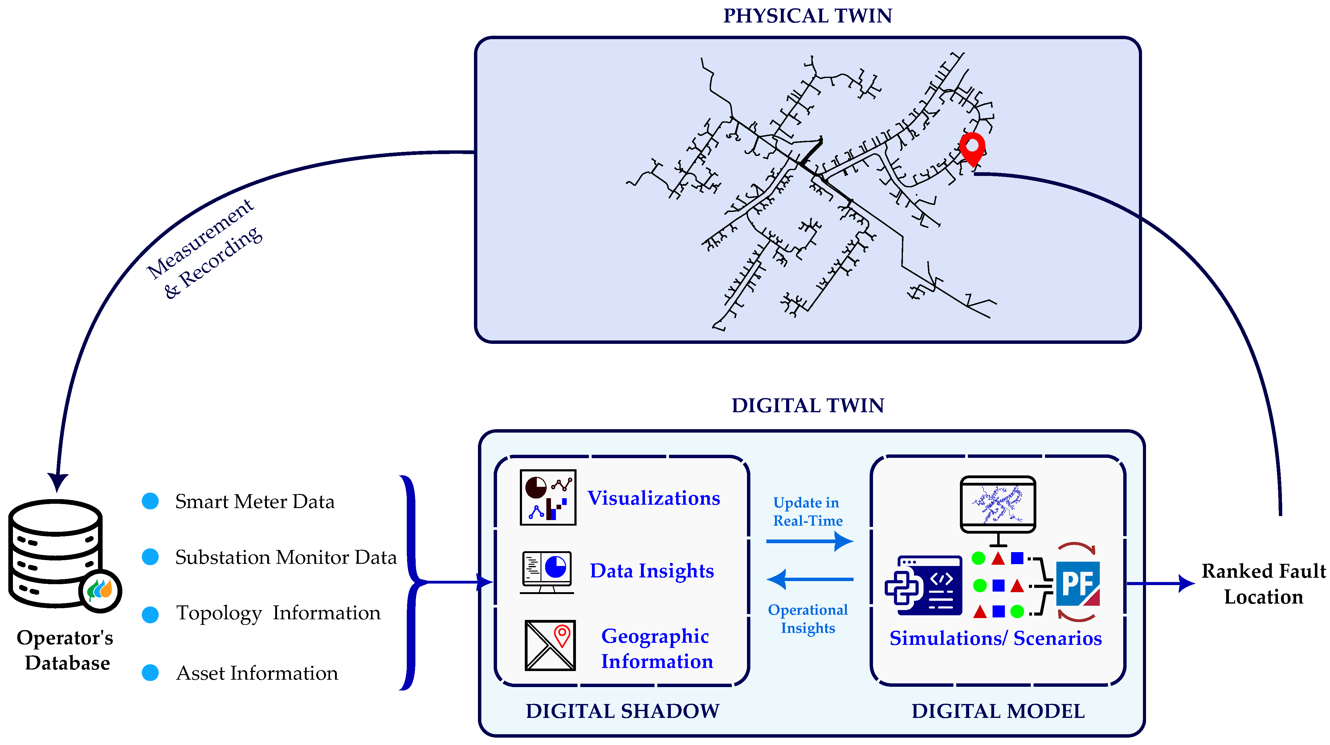
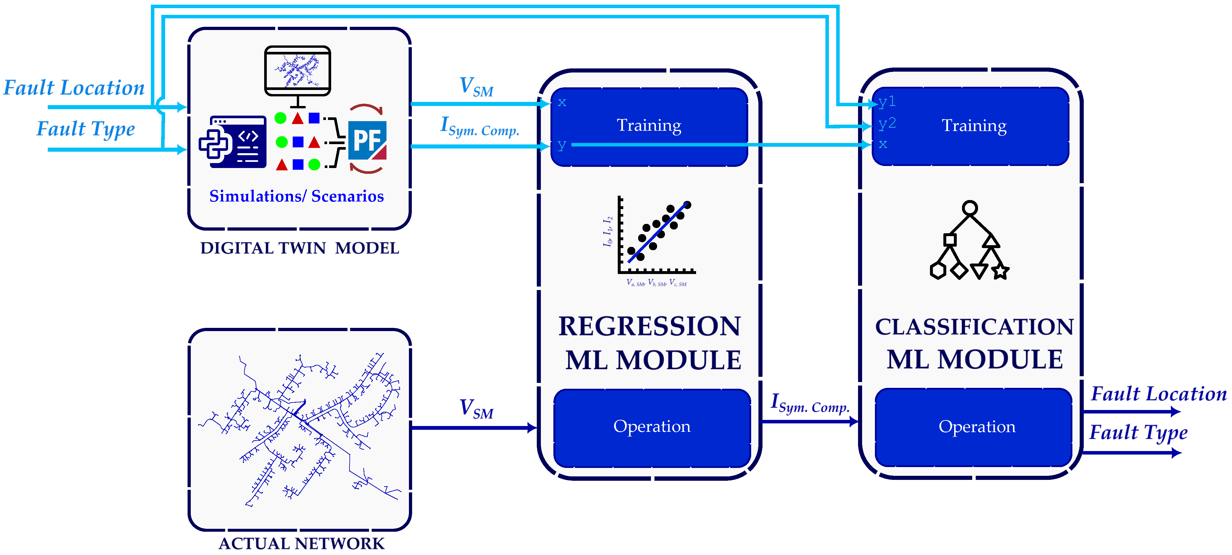
2.1. Overview of the Proposed Digital Twin

Considering that, by utilising the data from smart meters and attaining the knowledge of the characteristics and topology of any distribution network, a precise DT of it can be built. The DT encompasses all pertinent network information, including load demand, distributed generation unit type and rating, cable characteristics, as well as the location of protection and monitoring devices, such as fuses and smart meters, respectively.
As represented in Figure 1, the discussed DT concept can be partitioned into a digital shadow and a digital model [51]. The digital shadow represents the real-time monitoring of incoming data streams; these can be smart meter data feeds of voltage time-series, substation monitor voltages, and the power time series that are being recorded at each sampling time (e.g., half-hourly). The insights of this digital shadow, along with the known topology and cable data, are used to synthesise and tune the digital model. The digital model is then used to simulate the underlying network. It should be noted that this DT partitioning ensures that the digital model is continuously updated to capture the most recent network structure and characteristics. From there, the developed DT is utilised to perform hundreds of what-if scenarios on the underlying network, and this is performed without affecting its physical counterpart and while using and recording the results to improve the planning, prevention of issues, and optimising the operation of the network [52]. This DT has the capability to simulate network behaviour under different scenarios, such as faults, and it can train ML algorithms for fault identification and location.

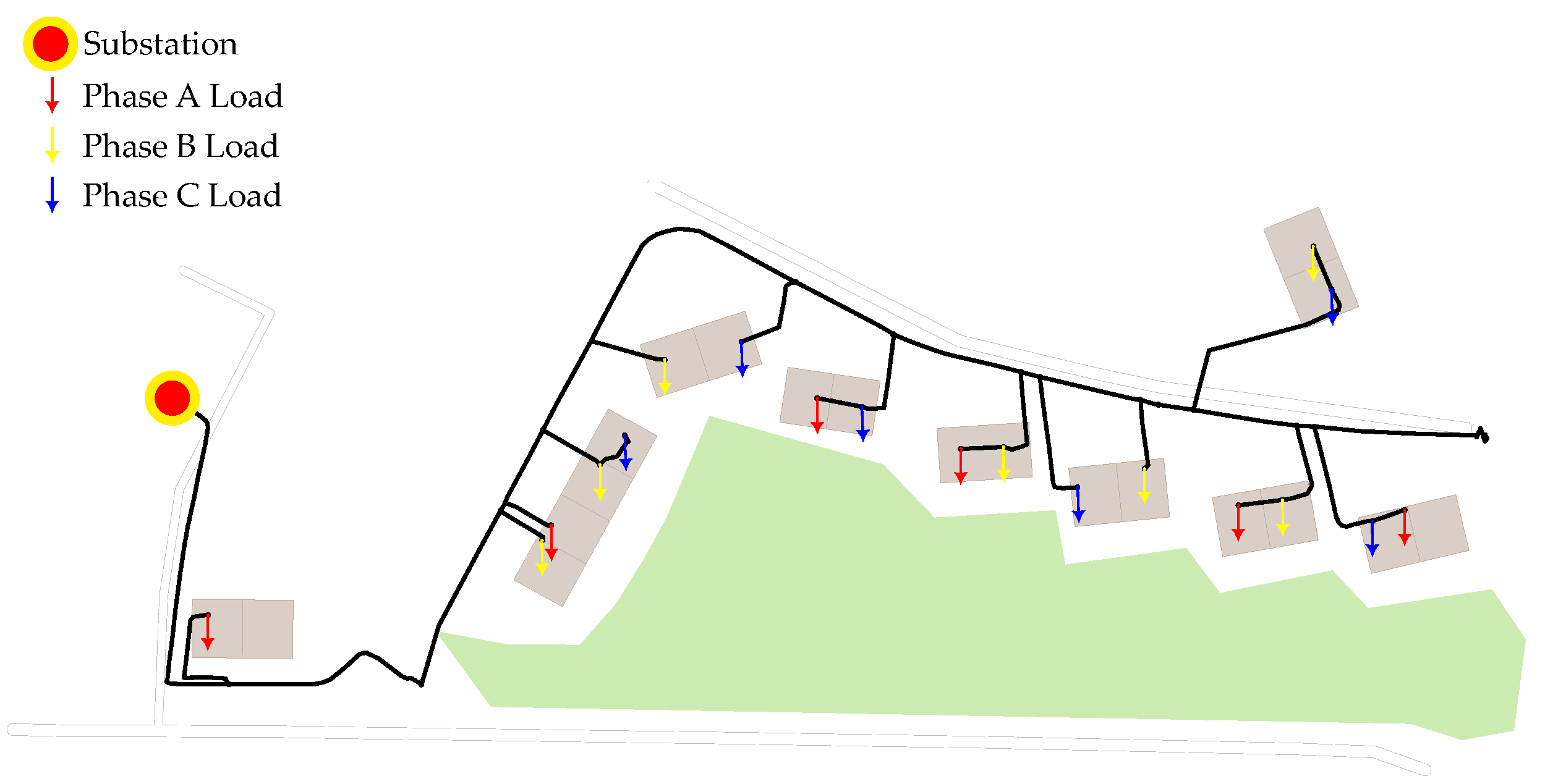
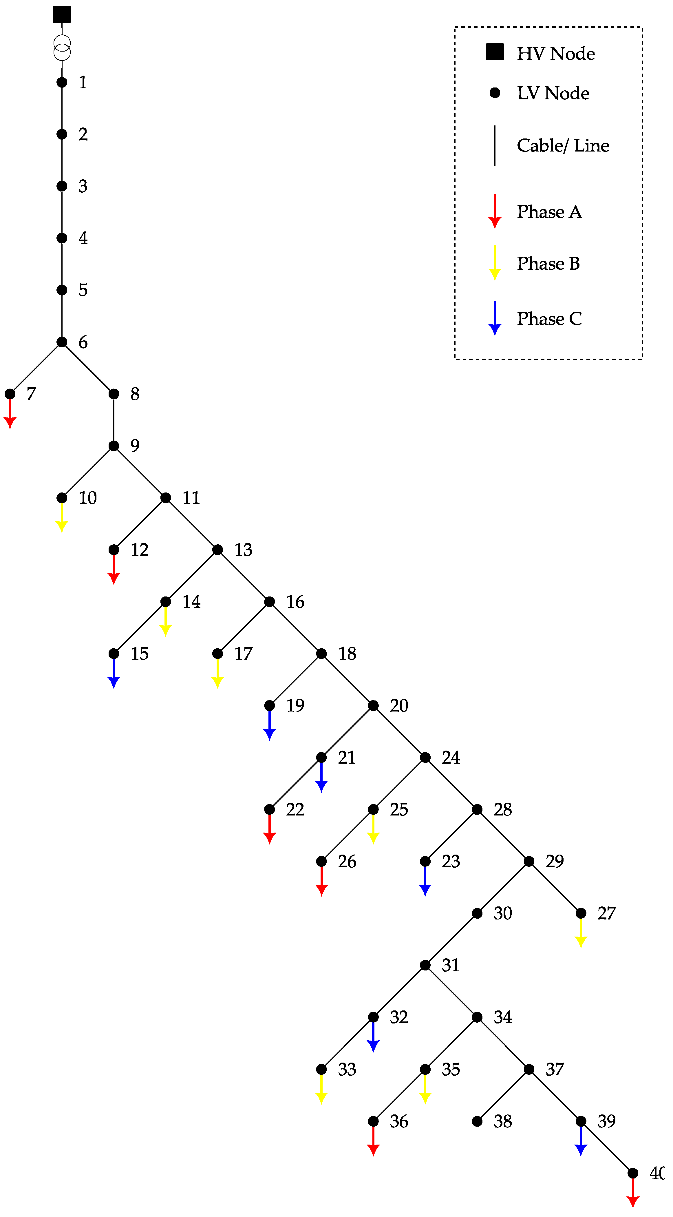
2.2. Scottish Power Energy Network-Based Digital Twin

To validate the proposed method’s practicality, a distribution feeder within the operation area of Scottish Power Energy Networks (SPEN), a Scottish DNO, was employed to build the DT model. The depicted network, as outlined in Figure 2, comprises a low-voltage LV feeder that derives its supply from a substation’s 11 kV/0.4 kV transformer. This feeder system encompasses a total of 41 distinct nodes, and it is interconnected by 39 separate cables, all of which collectively serve a customer base of 19 households. In SPEN’s LV support room [53], the SM data are visualised on a geographic map to help operators locate network incidents, and this can be thought of as a version of the digital shadow discussed in the previous section. However, for analysing different network study scenarios or simulating different events, a digital model is required. Hence, as part of this research, the network topology and intrinsic characteristics of this feeder were extracted from the databases of SPEN, thereby allowing for establishing an accurate digital model as part of the DT in DIgSILENT PowerFactory 2023 software package. In the PowerFactory Model, 19 loading points were modelled as low-voltage single-phase loads that were distributed between the three phases. In addition, in the created model, all customer (LV loads) voltages were measured through SMs, which was achieved without measuring the power demand to match the realistic operations since individual customers’ power demand was considered confidential and was unavailable to the DNOs in the United Kingdom (UK), in accordance with General Data Protection Regulation (GDPR). This lack of power measurement imposed an additional challenge for SPEN in fault localisation. In order to avoid using and releasing any confidential and private data, four loading conditions were estimated to mirror real-world scenarios. Loading conditions were estimated based on aggregate feeder consumption. Additionally, SM readings were concurrently generated alongside the established synthetic loads, further enhancing the model’s fidelity and practicality. Ultimately, the resulting feeder model structure was delineated in the tree representation of the feeder’s model, as illustrated in Figure 3. This representation encapsulates the interconnected nodes (buses), branches (cables), and the associated loads, indicating their respective connections within the distribution network.

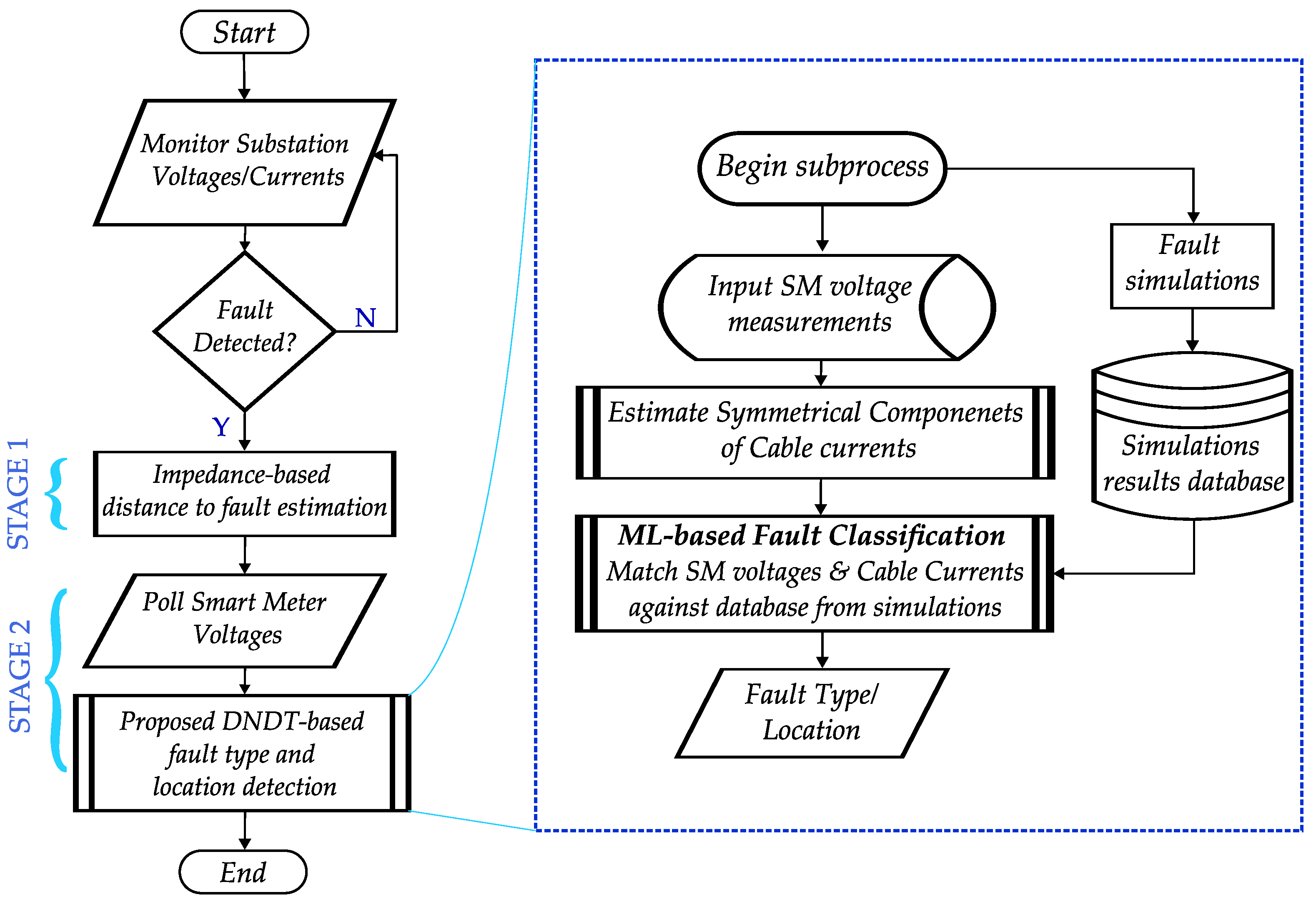
2.3. Proposed Two-Stage Fault Detection, Identification, and Location

The main assumption for the proposed fault detection method is that DNOs can autonomously acquire voltage readings from SMs within a designated area if the voltage violates a particular threshold, or, upon certain substation events, the voltage readings and status reports can be polled from the connected SMs in the impacted feeder. This also includes the added capability to request voltage readings at a higher sampling for these affected SMs when necessary; this assumption is per the Smart Metering Equipment Technical Specifications (SMETS) [33], which sets the specifications of all SMs in the UK. The key contribution of the suggested technique is its capability to identify and locate faults within LVDN when solely using SMs data, thus eliminating the need for extra high-sampling devices such as μ PMUs. However, due to SM’s relatively long sampling period (usually 30 min) and the instantaneous nature of faults, a two-step fault detection approach was adopted. In the initial stage, the conventional substation monitor captures power/voltage disturbances, computes corresponding fault impedance, and triggers the second data-driven stage. In the second step, SMs status and readings for the affected feeder are polled using the highest sampling rate technically viable by the communication infrastructure (typically 10: 30-s sampling [33]). This information is then employed as the input for the proposed Distribution Network Digital Twin (DNDT)-based fault localisation algorithm. As illustrated in Figure 4, the flow chart captures the high-level structure of the proposed DNDT-based fault detection and localisation. The substation monitor keeps track of voltage and current levels to detect faults and disturbances before they happen. If a developing pre-fault condition is detected, an impedance-based method is used, along with polling time-series voltages and alerts from SMs in the affected feeder. These polled SMs voltages are then fed into the pre-trained fault type detection and localisation models. This is a data-driven stage, where the SM voltages from the pre-fault incident are used to estimate the network’s CSC. Then, the measured voltages and estimated currents are set against a database of fault locations to estimate the matching type and location. The implementation details of this data-driven stage are discussed in Section 2.4.

2.4. Fault Identification ML Features Engineering

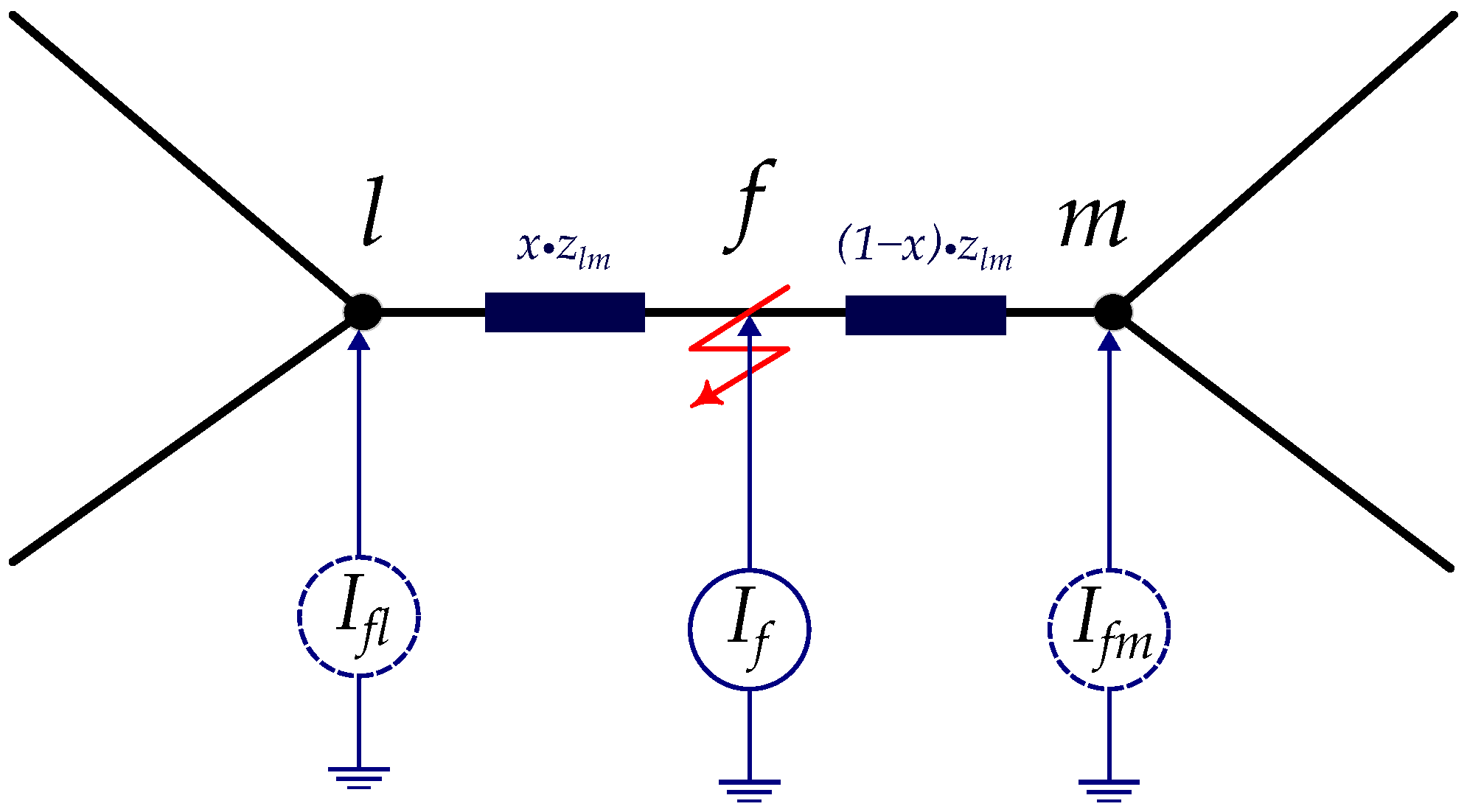
2.4.1. Smart Meter Voltages and Cables’ Current Symmetrical Components

As unsymmetrical faults, particularly Single-Line to Ground Fault (SLGF), constitute the majority of faults in a distribution network, the symmetrical components of cable currents can be regarded as a reliable predictor of fault locations [54,55,56]. Figure 5 shows a case of a fault occurring in an arbitrary fault location f at a distance per cent x from node l. Assuming that the cable impedance is equally distributed through the cable, and that a total cable impedance of z l m is between nodes l and m, the impedance between node m and the fault point f can also be referred to as ( 1 x ) · z l m . From network analysis, the fault current at point I f can be split into two equivalent injections at nodes l and m, as in Equations (1) and (2), respectively.
I f l = ( 1 x ) L I f
I f m = ( x ) L I f
In the case of an unsymmetrical fault, such as a phase A to ground (A-G) fault, the negative sequence current vector I a 2 at all network nodes exhibits a valuable feature that is suitable for the identification of fault type and location. This feature can be shown by (3), which dictates that, during a fault, the negative sequence currents I a 2 are zero-valued for all network nodes, except for those pertaining to the fault location, where non-zero values exist.
I a 2 = [ 0 0 I f l I f m 0 0 ] T
However, given the absence of current measurements—let alone the required phasor measurement needed for analysing negative sequence components—in the LV cables (where solely RMS voltage measurements are accessible through SMs readings with a low sampling), a data-driven feature extraction methodology was proposed based on the simulation capability of DNDT, as shown in Section 2.4.2

2.4.2. Data-Driven Feature Extraction

The general approach to attain symmetrical components from network voltages analytically can be laid off as follows (starting by attaining the voltage symmetrical components in Equation (4)):
V a V b V c = 1 1 1 α 2 α 1 α α 2 1 V a 1 V a 2 V a 0 V P = A V S
where V P represents the Root Mean Square (RMS) voltage readings, A is the transformation matrix with the complex number operator α = e j 120 , and V S is the calculated symmetrical components. Hence, the voltage symmetrical components can be attained through the inverse operation in Equation (5),
V S = A 1 V P
Then, with knowledge of the network’s negative sequence impedance Z , the negative sequence component of the currents can be attained as in Equation (6).
V a 2 = Z a 2 I a 2 Generally , V S = Z I S
However, in the practical case, only the RMS voltage magnitudes were measured by SM at a subset of the network nodes. This makes the previous analytical approach impractical in the case of LV feeders. In addition, the prior analysis demonstrated that the voltage readings V P can be deduced into the symmetrical current component vector I S through transformation matrix A and network impedance Z . These parameters change as per the fault type and location according to the network’s equivalent circuit of symmetric components for that fault. Here, the advantage of having the proposed DNDT arises as the ability to embed knowledge of these parameters and the estimation of unmetered node’s voltages through fault scenarios simulations of theDT model, as well as the production of a dataset constituted of all possible fault locations, types, and scenarios against the metered voltages and symmetrical cable components. This simulation-generated database can be inputted into a ML regression model to derive the symmetrical current components from SM voltages during faults as a first step. The second step would be to utilise the metered SM along with the predicted current symmetrical cable components to train a classification model that would be able to determine the fault’s type and location. The simulation, training, and operation stages of the proposed ML-based model are shown in Figure 6.
From Figure 6, it can be seen that the DT’s model was used to simulate different fault scenarios with different fault types and locations, and then the resulting RMS voltage readings were captured from the SMs in the network. And because the digital model was not limited by the actual network’s measurement limitations, additional information about the coinciding symmetrical voltage and current components can be recorded for each simulation, thus creating a unique dataset of SM voltages and their corresponding symmetrical components for this network. This dataset was then used to train a ML model that acts as a transformation model to convert SM’s RMS voltages into the corresponding cables’ symmetrical current components. The resulting symmetrical components were then used in addition to the SM voltages in the fault identification, which was achieved through ML-based classification modules to determine the type and location of the fault.

3. Simulation, Data Preparation, and ML Model Training

In this section, the outcomes of the proposed fault identification and location methodology are presented for the Scottish LV feeder. For the studied feeder, the substation fuse would immediately blow for solidly high-current short-circuit faults. However, high-impedance shunt faults or faults with open conductors are not usually detected as they develop, even though they may cause customer interruptions and hugely impact power quality [57]. These faults are more difficult to locate within the LV feeder using traditional techniques [58,59]. Therefore, this study primarily focuses on high-impedance shunt faults and open conductor faults.

3.1. Fault Scenario Design

To evaluate the performance of the proposed fault identification and localisation methodology, a comprehensive set of fault scenarios was systematically designed. These scenarios were generated by iteratively varying parameters to simulate a wide range of possible fault conditions. The following variations were applied to each cable within the network.

3.1.1. High-Impedance Shunt Fault Scenarios

For high-impedance shunt fault scenarios, the faulted cable, fault location percentage of the total cable length, fault type, phase, fault resistance, and system loading level were systematically varied as follows:
  • Faulted cables: The study encompassed faults occurring in all 39 cables of the feeder, with each cable subject to the following variations.
  • Percentage of faulted cable length: Fault scenarios were generated with varying percentages of the faulted cable length, ranging from 0% to 100% at 10% intervals.
  • Fault types: Four distinct high-impedance shunt fault types, i.e., Line to Ground (LG), Line to Line (LL), Line to Line to Ground (LLG), and Three-Phase (3Ph) faults were considered.
  • Faulted phases: Faults were induced in each of the three phases (A, B, and C) individually to account for the faults at different phases.
  • Fault resistance ( R f ): A range of fault resistances (in ohms) was employed to emulate the different fault conditions, with values of (0.2, 0.3, 0.4, 0.5, 0.6, 1, 1.5, 2, 3, and 5) k Ω . These values were chosen to emulate the case of high-impedance shunt fault values.
  • System loading: Four different system loading conditions were considered, with values of [0.5, 0.9, 1.5, and 2] kW. These represented different levels of network utilisation for the given feeder. The implied range takes into account the yearly and daily system loading variations.

3.1.2. Open Conductor Fault Scenarios

The open conductor faults can be considered a special case of the high-impedance shunt fault, where supply to the rest of the network was cut; hence, it has similar variations as follows:
  • Faulted cables: Similarly, the open conductor analysis was performed on all of the 39 cables in the network.
  • Percentage of faulted cable length: Unlike the case of high-impedance shunt faults, the percentage of the cable at which the open conductor fault occurred did not have a significant impact on the readings; however, the results were augmented with varying percentages of the faulted cable length, ranging from 0% to 100% at 10% intervals.
  • Faulted phases: Open conductor fault scenarios covered all of the permutations of a single-phase outage (A, B, and C) and of the phase combinations (AB, BC, AC, and ABC).
  • System loadings: The same four system loading conditions (0.5, 0.9, 1.5, and 2) kW were utilised to capture the impact of varying network utilisation on fault identification and location.

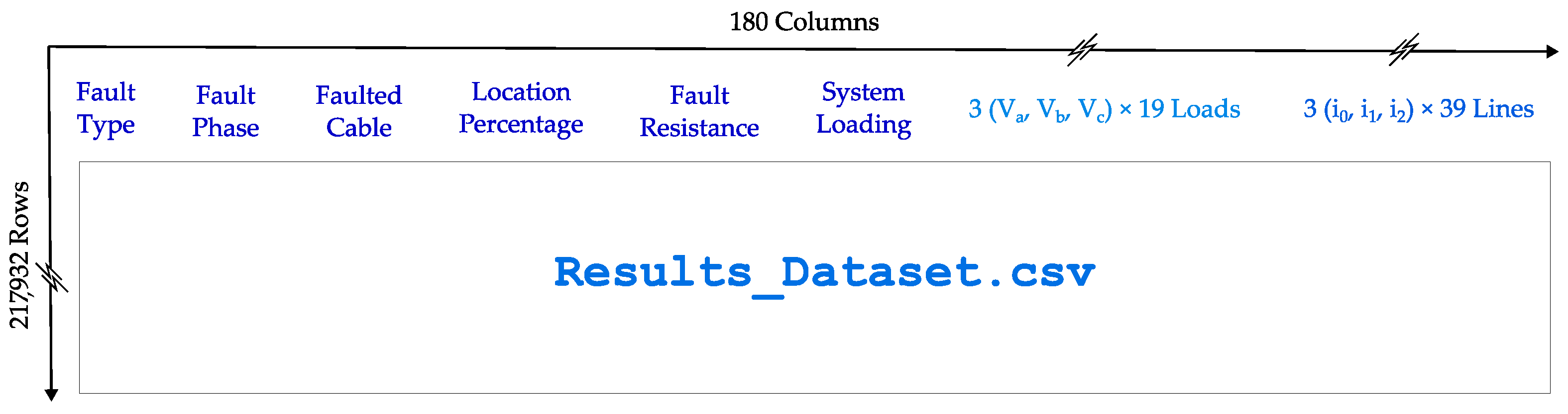
3.2. Simulations and Training Dataset

The aforementioned parameter variations and values were incorporated into a Python script, thereby facilitating the automation of the DIgSILENT PowerFactory model for the entire feeder. The Python script was structured as in Algorithm A1 in Appendix A, which shows that it loops through the given range of fault parameters through the indented levels of loops that, at the end, adds to the recorded relevant measurements, including SMs readings and the cables’ CSCs into a dataset CSV file Results_Dataset.csv. The resulting dataset, as visualised in Figure 7, had 217,932 rows (which corresponded to the permutations of different fault scenarios) and 180 columns. The columns included the following:
  • The first 6 columns were for defining the fault scenarios: fault type, phase, cable, location percentage, fault resistance, and loading.
  • The following 57 ( 3 × 19 ) columns were for the A, B, and C RMS voltage values for each of the 19 loadings, where only the connected phase had a null value for the other two phases.
  • The remaining 117 ( 3 × 39 ) columns corresponded to the currents’ zero, positive, and negative sequence components ( i 0 , i 1 , i 2 ) for each of the 39 cables.
Figure 7. Structure of the training dataset.
Energies 16 07850 g007

3.3. Machine Learning Models

3.3.1. Value of the Current Symmetrical Components’ Estimation Stages

The initial approach was to directly use a ML classification model to map between the SM voltage-only readings into the corresponding fault type and location; however, when using that approach, the accuracy plateaued at 70.7%. Figure 8 displays a fault located at cable “L 28-29” on the feeder. The impedance-based method, when applied to this scenario (as an impedance measured from the substation), resulted in multiple potential fault locations due to the radial nature of the feeder. These estimations were further affected by the high-impedance characteristics of the fault, thus causing an offset from the true fault location. In contrast, when utilising the initial approach of the raw SM voltages only as inputs for the ML classification model, the accuracy was notably low, and it misclassified the fault location to cable “L 31-34”. The voltage-based model notably misclassified the faults situated upstream or at a distance from the SM locations. This limitation prompted the development of the proposed CSC-based method, which successfully located the studied fault to the true location. The CSC-based accurately identified the location of faults, even in cases where the traditional voltage-based method struggled and achieved an overall accuracy of 95.77%. This enhancement not only showcases the efficacy of the CSC-based approach, but it also underscores the crucial role of having a DT that is able to predict these CSC on basis of the network’s model.
In the subsequent subsections, the trained ML models were validated through thousands of scenarios. A confusion matrix was employed to succinctly represent all cases, with the actual locations (true class) delineated in the rows. For each true case, the corresponding row provides a breakdown of how many validation scenarios were classified into each category (predicted class). This visualisation aids in the comprehensive evaluation and understanding of the classification accuracy and weakness.

3.3.2. Load Voltage/Cable Current Regression Model

As Section 2 outlines, the fault identification and location process relies on the cables’ CSCs. Given that SMs provide voltage magnitudes only, a regression model was imperative to derive the zero, positive, and negative sequence currents of the network cables. It is worth noting that this regression model is unique to each specific feeder, and it corresponds to its respective impedance characteristics. For this study, a Random Forest Regressor was trained on the 19 SM voltages of the loads as the input, and the cables CSCs as the output. After training, the regression model was evaluated through a five-fold cross-validation using the entire dataset to benchmark the regressor’s accuracy. The validation showed a satisfactory Mean Squared Error (MSE) of 3.58 × 10 5 , which presents the trained model’s ability to accurately predict the entire network’s CSCs from the provided SM voltages.

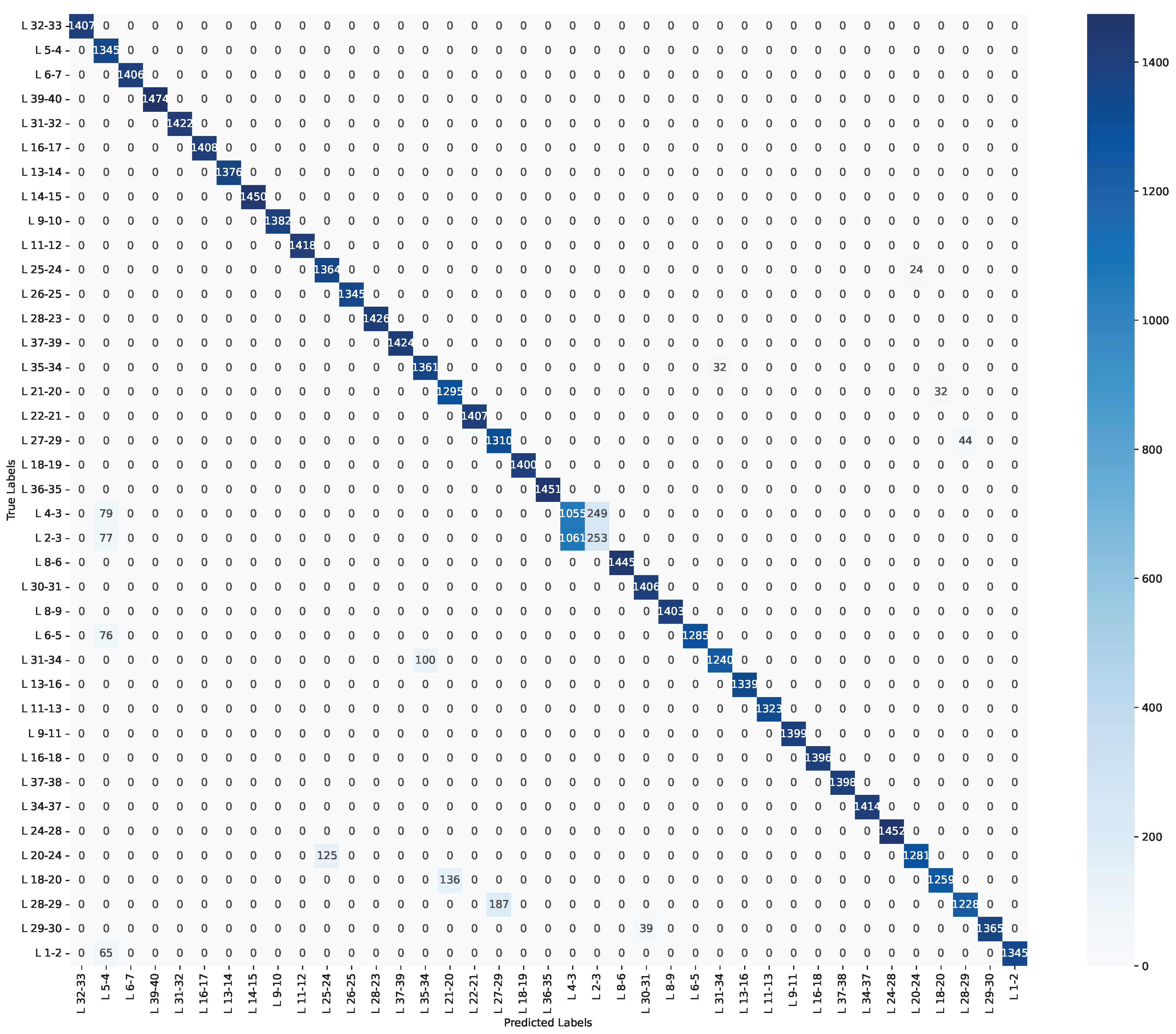
3.3.3. Fault Location Classification Model

Considering the relatively short lengths of the sections/cables in the analysed LV feeder (as shown in Table 1), predicting the fault cable alone can suffice in fully locating a fault. To achieve this, a Decision Tree Classifier was trained on the voltages and the CSCs from the simulation-generated dataset. Utilising a 25% holdout for verification, the classifier demonstrated an accuracy of 95.77%, which is visualised by the confusion matrix in Figure 9. This matrix was deemed acceptable given the cables’ close proximity and limited length. For instance, the model exhibited a higher degree of confusion in distinguishing the faults between cables “L 4-3” and “L 2-3”; however, Table 1, along with Figure 3, clarify that this is attributed to the fact that cable “L 2-3” can be viewed as a mere 20 cm extension of cable “L 4-3”. In Figure 9, the confusion matrix reveals an important observation: cables near or surrounded by smart meters are more accurately located compared to cables that are farther away. We can see this by examining the true positive (diagonal) numbers in Figure 3 and Figure 9. For instance, the nodes at the beginning of the cable, like L 4-3 and L 2-3, had the highest confusion and lowest true positive values because they lacked nearby smart meters. On the other hand, the cables that were surrounded by smart meter-measured nodes, such as L 39-40 and L 14-15, had the highest true positive rates. This demonstrates the impact of smart meter locations on the accuracy of fault cable detection.

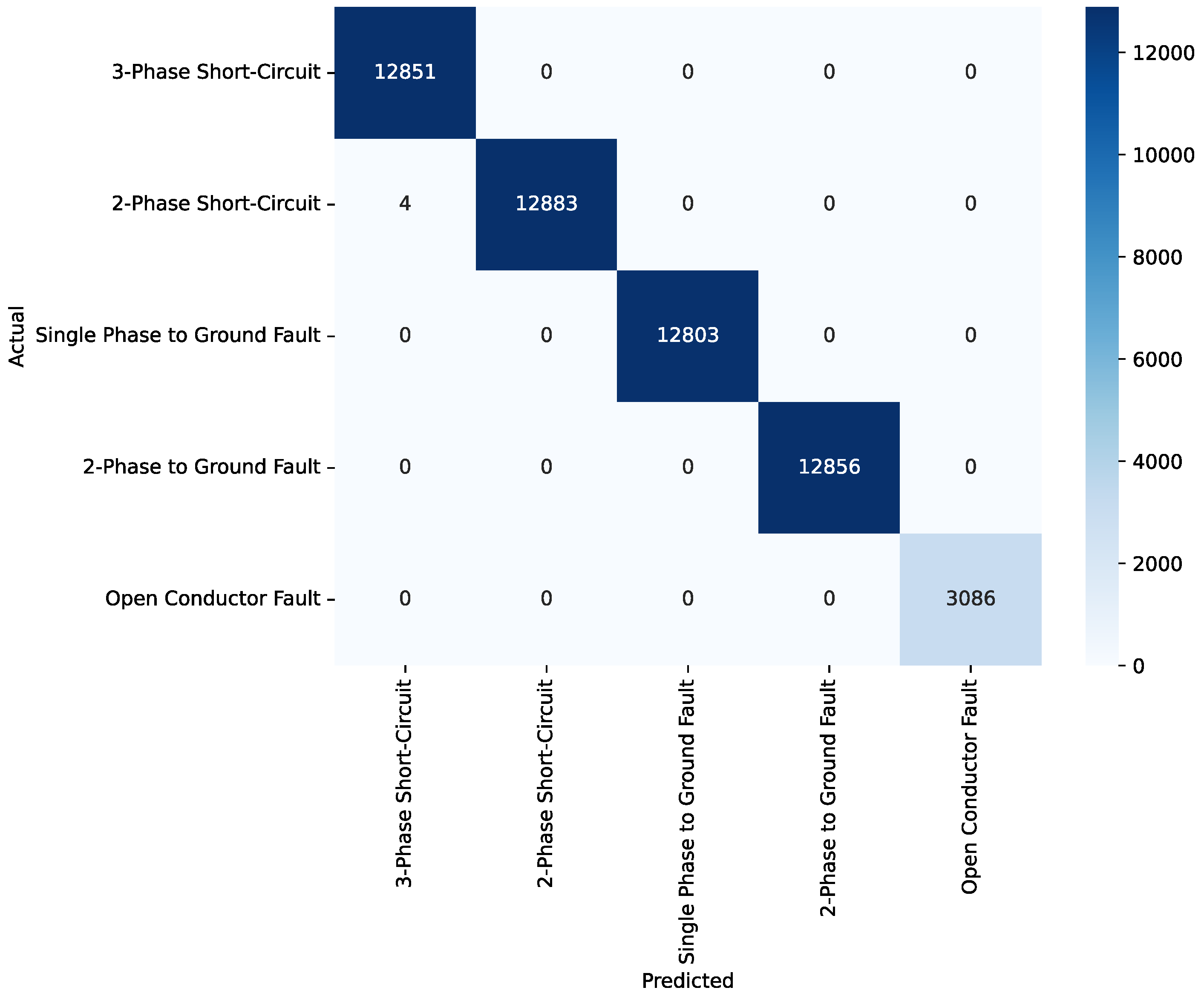
3.3.4. Fault Type Identification Classification Model

A Decision Tree Classifier was employed to predict the fault type, an essential step for fault identification. The original dataset was utilised in its training, thereby incorporating all voltage and CSC, as outputted from the simulation into their raw form. However, for a realistic validation, only the voltages of the 25% holdout set were employed. Subsequently, when using the previously mentioned regression model, the corresponding CSCs were predicted. These predicted CSC values, along with the actual measured voltages, were used as inputs for validation. The results demonstrated an exceptional accuracy of 99.9%. The confusion matrix for the fault type classifier validation is depicted in Figure 10.

3.3.5. Detailed Overview of Machine Learning Models

(a)
The Random Forest Regressor
As discussed in Section 3.3.2, the Random Forest Regressor, a powerful ensemble learning technique, was employed to estimate the CSCs based on the measured SMs voltages. A Random Forest Regressor is an ensemble learning method that leverages the collective insight of multiple decision trees to make accurate predictions. It operates by aggregating the predictions of numerous individual trees, each trained on different subsets of the data. The key parameters considered for this model include the number of trees in the forest (n_estimators), the quality metric for splitting nodes (criterion), and the maximum depth of the trees (max_depth).
For the implementation, the Random Forest Regressor from the Sci-Kit Learn library [60] was utilised. The specific parameter were carefully chosen to enable the model to effectively handle fault identification and localisation tasks in real-time scenarios. The complete set of the trained model’s parameters is outlined in Table A1 for reference.
(b)
Decision Tree Classifier for Fault Type and Location
A Decision Tree Classifier is a machine learning algorithm that makes decisions by splitting the dataset into subsets based on the value of the input features. It recursively partitions the data until it reaches leaf nodes, which represent the final decisions or classifications. The Decision Tree Classifier was chosen for fault type and location classification due to its inherent interpretability. This means that the model’s decision-making process can be easily understood and visualised, which is crucial in critical applications like fault diagnosis. The DecisionTreeClassifier class was used from the Sci-Kit Learn library [60] with the parameters being configured as displayed in Table A2.

4. Results and Discussion

In order to estimate the holistic accuracy of the proposed approach, the original DIgSILENT PowerFactory model was again used to simulate 100 test scenarios, whose conditions from fault location, type, and resistance were randomised. Then, the SM voltages were captured and inputted into the pre-trained ML models in order to attain a predicted fault cable location and type. The test fault scenarios were designed to be more general than the training scenarios. This demonstrated the machine learning capability to generalise from the training data and to make predictions for fault locations that were not specifically encountered during training. For the type classification, the model achieved an outstanding accuracy of 100% in determining the fault type. On the other hand, for cable location, an accuracy of 78% was found. However, this accuracy stands for the exact matches between the correct cable and predicted cable, as displayed in Table 2, but it can also be seen that even those miss-classified cables were geographically close to each other; hence, an additional distance error was used to capture the distance between the predicted cable’s midpoint and the correct cable’s midpoint to give an indication of the classification error in terms of distance. The histogram displayed in Figure 11 shows clearly that, although the spot-on accuracy was 78%, 87 of the 100 test cases had a distance error between 0 and 0.02 km, with only 6 cases that had a distance error between 0.02 to 0.04. In addition, only 6 cases had a distance error between 0.04 to 0.06. Out of the 100 cases, only 1 case had a distance error above 0.06 km.
In the context of fault location within distribution networks, the achieved results hold significant promise. Relying solely on SMs for fault identification and localisation represents a shift towards the more efficient and cost-effective monitoring strategies that were only enabled by the DT model. The exceptional fault type classification accuracy of 100% underscores the robustness and added value of the proposed initial stage of the CSC estimation from the SM voltages. Meanwhile, for fault location, 99% of the predicted locations were at a relatively close geographic proximity to the actual fault location. This makes the proposed methodology helpful in the automated detection of faults and their types, and it helps with narrowing down the search area into a specific cable section. This, in turn, will lead to much less connectivity disruptions for customers and will improve the efficacy of maintenance teams being dispatched to the fault location.

4.1. Detection of Multiple Faults

While the proposed algorithm exhibits remarkable efficacy in identifying individual faults, it is designed with real-time applications in mind. This ensures that, once a fault or network topology change is recorded, the DT undergoes a prompt event-based update process. This includes the retraining of classification models to accurately reflect the latest network configuration, thereby incorporating any existing faults. This dynamic approach allows for the system to operate with the most up-to-date information, as well as to identify and record multiple faults as they occur sequentially. The other potential approach to achieve multiple or simultaneous fault identification could be through the exhaustive simulation of all the potential permutations of simultaneous faults in the initial training dataset; however, this would be significantly computationally extensive, as the larger network size may lead to higher confusion for the classification models.

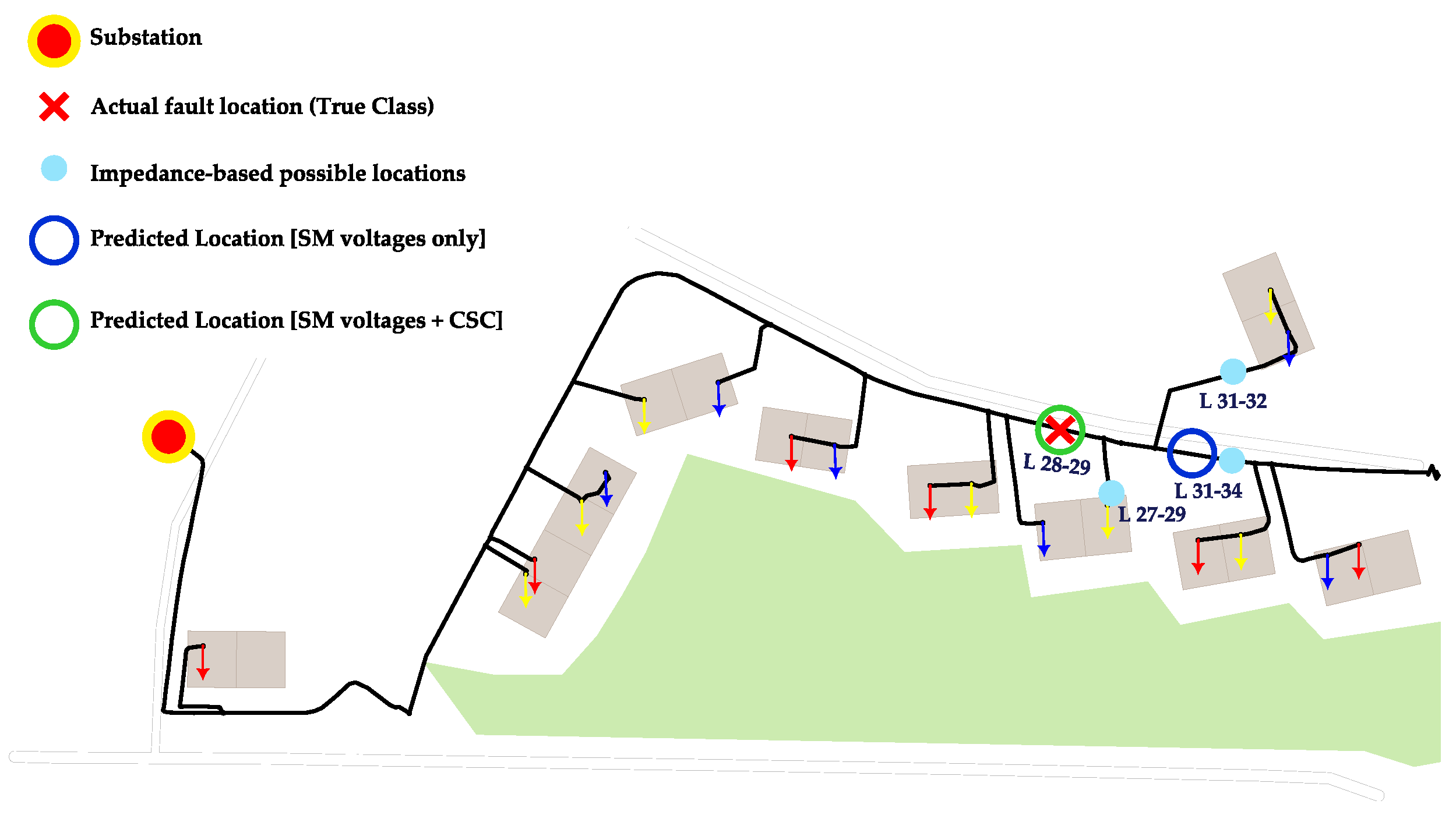
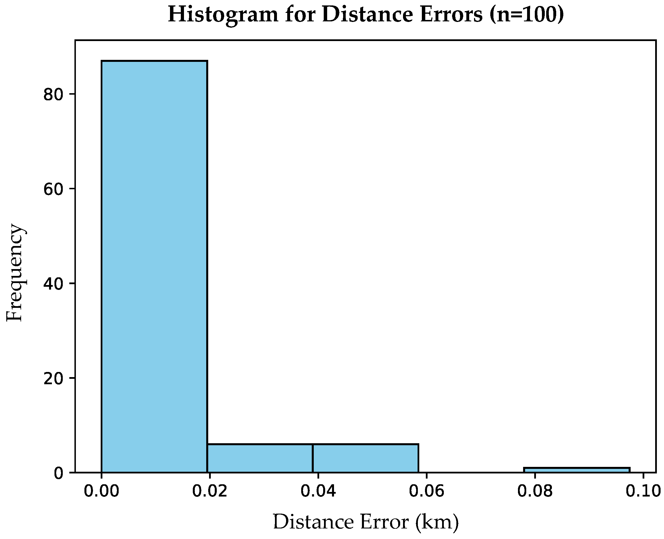
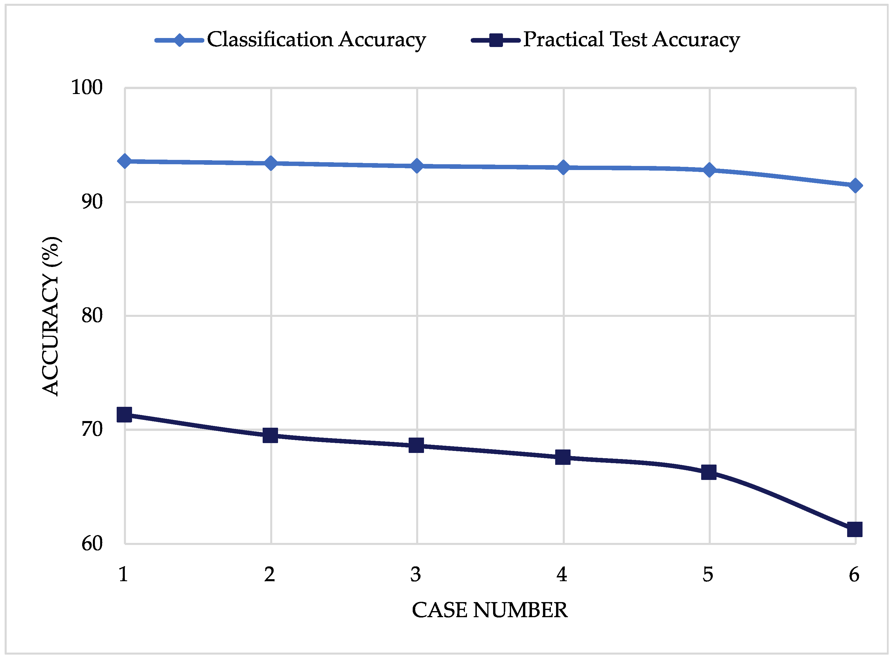
4.2. Impact of the Partial SM Coverage on Fault Localisation Accuracy

In this section, the 100 test case scenarios were re-simulated to understand how the accuracy of the proposed method is affected by the partial coverage of SMs. These values were based on the distribution of the partial smart meters, as shown in Figure 12. In the initial case previously studied in Case 1, where 19 out of the 19 possibly available SMs were connected (19/19), there were no crosses that indicated the SMs was unavailable. In Case 2, 4 unavailable SMs were found, which meant that measurements were collected from only 15 of the smart meters (15/19). In both Cases 3 and 4, only 13 connected SMs were featured, the difference being that, for Case 4, the disconnected SMs were the lateral ones, which caused less visibility for the voltages. Moreover, the low-coverage Cases 5 and 6 featured only 9 and 6 SMs, respectively, which represented the low SM penetration scenarios.
In the previously studied cases, Case 1 demonstrated full connectivity with 19 out of 19 SMs (19/19), as well as the highest classification accuracy of 93.6%. However, Case 2 enclosed 4 unavailable SMs, which resulted in a data collection from only 15 out of 19 m (15/19), thus leading to a slight drop in the classification accuracy to 93.4%, which is comparable to the previously calculated in Section 3.3.3. Both Case 3 and Case 4 had 13 connected SMs, but, in Case 4, the disconnected meters were located on the laterals, thus resulting in reduced visibility and, consequently, a slightly lower classification accuracy of 93.03% as opposed to 93.2% for Case 3. Furthermore, for low SMs coverage, Case 5 and Case 6 represented scenarios with 9 and 6 smart meters, respectively, thus indicating low smart meter penetration, as they exhibited a classification accuracy of 92.8% and 91.5%, respectively. Figure 13 presents the classification accuracy, which was determined using the training dataset for validation, as well as the practical test accuracy, which was assessed by employing random real-world scenarios from the training dataset for testing in all of the six cases. These results suggest the significant impact of the number and location of the connected SMs on the fault localisation accuracy. Although the classification’s validation accuracy remained above 90%, the realistic tests showed a significant drop in accuracy with partial SMs coverage. In addition, the drop between Cases 3 and 4 were shown to be much higher for the test scenarios, thus validating the importance of having SMs dispersed through the lateral nodes of the network. This alludes to the recommendation of having a minimum lateral node coverage of 70% to ensure reliable accuracies.
It is worth mentioning that the accuracies and values presented in this study are directly tied to the specific characteristics of the analysed network, and they are limited to the studied high-impedance pre-fault identification, which underscores the importance of contextual considerations. Nonetheless, they serve as compelling evidence of the viability and effectiveness of the proposed DT-based methodology for fault identification and localisation. It is crucial to acknowledge that the performance metrics and model training outcomes may vary depending on factors such as network size, the density of deployed SM, and the prevailing operating conditions.

5. Conclusions

This paper introduced a pioneering methodology for detecting high-impedance shunt faults and open conductor faults in DN feeders. By integrating state-of-the-art DNDT technology with SM measurements only and without μ PMUs, particularly voltage-magnitude readings, fault detection capabilities for DNOs increased significantly. Initial attempts relied solely on the SM-based voltage-only approach, which yielded an accuracy of 70.7% in fault type and location classification. However, by incorporating the line CSC through a machine learning-based regression method within the DT framework, fault localisation and identification accuracy surged to an impressive 95.77%.
Through extensive DT simulations encompassing a spectrum of fault scenarios, the trained ML models exhibited exceptional performance. Fault type classification achieved a flawless 100% accuracy rate, thereby showcasing the robustness of the approach in distinguishing the various fault types. Additionally, the predicted fault locations demonstrated remarkable proximity, whereby they deviated by less than 0.06 km from the actual fault location in 99% of the tested cases. This remarkable precision substantially reduced the area requiring investigation, thus enabling targeted dispatches of maintenance teams and minimising customer disruptions.
These results represent an advancement in the fault detection within DN. The integration of the CSC estimation stage from the SM voltages signifies the value of building a DNDT for attaining additional information, as well as for obtaining insights from raw SM voltage-based DT simulations. In light of the analysis highlighting the crucial role of accelerating the SM roll-out program, it becomes evident that expediting these efforts is essential for maximising additional benefits and enhancing the efficiency of applications, particularly in areas such as fault localisation.
In summary, the proposed methodology equips DNOs with a SM data-informed fault detection, whereby there is high confidence in specifying the fault type and in providing precise geographic areas for investigation.
The DNDT research opens up new avenues for optimising the operation of active distribution networks. Having a DT in the network empowers broader operational capabilities within diverse distribution network contexts, thus ultimately contributing to enhanced reliability and resilience. Future investigations may focus on testing the methodology with different feeders of diverse network configurations and operational environments. Additionally, an extension of this work could involve pre-fault identification and locations that use a partial coverage of SM, or a high integration of embedded generation.

Author Contributions

Conceptualisation: M.N. and A.A.A.; Methodology: M.N. and A.A.A.; Software: M.N.; Validation: M.N. and F.A.-V.; Formal analysis: M.N.; Investigation: M.N., A.A.A. and M.E.F.; Resources: M.N.; Data Curation: M.N. and F.A.-V.; Writing- original draft preparation: M.N. and F.A.-V.; Writing- review and editing: M.N., F.A.-V. and A.A.A.; Visualisation: M.N. and A.A.A.; Supervision: A.A.A., M.E.F. and E.E.; Project administration: A.A.A. and M.E.F.; Funding acquisition: A.A.A. and M.E.F. All authors have read and agreed to the published version of the manuscript.

Funding

This research was funded by the Energy Technology Partnership (grant number 201) and Scottish Power Energy Networks.

Data Availability Statement

The data presented in this study are available on request from the corresponding author and upon approval of the industrial partner. The data are not publicly available due to the sensitivity of data provided by SPEN.

Acknowledgments

This research was conducted in collaboration with LV Support Room at SP Energy Networks. Special thanks to Gary MacDonald (Lead Electrical Project Engineer, SAP) and James Yu MBE (Head of Future Energy Networks), who were both from SP Energy Networks, for their technical support to the project and provision of the distribution network data and topologies.

Conflicts of Interest

The authors declare no conflict of interest.

Abbreviations

μ PMUMicro-Phasor Measurement Unit
3PhThree-Phase
AMIAdvanced Metering Infrastructure
ANNArtificial Neural Network
CMLCustomer Minutes Lost
CSCCurrents Symmetrical Component
DNDistribution Network
DNDTDistribution Network Digital Twin
DNODistribution Network Operator
DTDigital Twin
GDPRGeneral Data Protection Regulation
LGLine to Ground
LLLine to Line
LLGLine to Line to Ground
LVLow Voltage
MLMachine Learning
MSEMean Squared Error
RMSRoot Mean Square
SLGFSingle-Line to Ground Fault
SMSmart Meter
SMETSSmart Metering Equipment Technical Specifications
SPENScottish Power Energy Networks
UKUnited Kingdom

Appendix A

Algorithm A1 Simulations’ automation and dataset building script
  • Require: Predefined arrays of fault Lines, types, phases, percentages, Rfs, loadings
  •     for type i n types do
  •         for phase i n phases do
  •             for Line i n Lines do
  •                for percentage i n percentages do
  •                    for Rf i n Rfs do
  •                        for loading i n loadings do
  •                            <PowerFactory Fault Event Simulation>
  •                            Add Fault parameters columns to row
  •                            Add SM voltages columns to row
  •                            Add lines CSC columns to row
  •                            add row to ’Results_Dataset.csv’
  •                        end for
  •                    end for
  •                end for
  •             end for
  •         end for
  •     end for
Table A1. Parameters for the trained Random Forest Regressor.
ParameterValueDescription
n_estimators10Number of trees in the forest
criterion‘mse’Quality metric for splitting nodes
max_features‘auto’Number of features to consider at each split
min_samples_split2Minimum number of samples required to split an internal node
min_samples_leaf1Minimum number of samples in newly created leaves
min_weight_fraction_leaf0.0Minimum weighted fraction of samples required to be at a leaf node
bootstrapTrueWhether bootstrap samples are used
oob_scoreFalseWhether to use out-of-bag samples for estimating generalisation error
n_jobs1Number of parallel jobs for fit and predict
verbose0Controls verbosity of tree building process
warm_startFalseWhether to reuse previous solution
Table A2. Default Parameters for Decision Tree Classifier.
ParameterValueDescription
criterion‘gini’Measure of split quality, possible values: (‘gini’, ‘entropy’, ‘log_loss’)
splitter‘best’Strategy for choosing splits, possible values: (‘best’, ‘random’)
min_samples_split2Minimum samples required to split a node
min_samples_leaf1Minimum samples required in a leaf node
min_weight_fraction_leaf0.0Minimum weighted fraction for a leaf
min_impurity_decrease0.0Minimum impurity decrease for splitting
ccp_alpha0.0Complexity parameter for Minimal Cost-Complexity Pruning

References

  1. BS EN 50160:2010+A3:2019; Voltage Characteristics of Electricity Supplied by Public Electricity Networks. British Standards Institute: London, UK, 2019.
  2. Silva, C.; Saraee, M. Understanding Causes of Low Voltage (LV) Faults in Electricity Distribution Network Using Association Rule Mining and Text Clustering. In Proceedings of the 2019 IEEE International Conference on Environment and Electrical Engineering and 2019 IEEE Industrial and Commercial Power Systems Europe (EEEIC/I&CPS Europe), Genova, Italy, 11–14 June 2019; pp. 1–6. [Google Scholar] [CrossRef]
  3. Densley, J. Ageing mechanisms and diagnostics for power cables—An overview. IEEE Electr. Insul. Mag. 2001, 17, 14–22. [Google Scholar] [CrossRef]
  4. Christie, R.; Zadehgol, H.; Habib, M. High impedance fault detection in low voltage networks. IEEE Trans. Power Deliv. 1993, 8, 1829–1836. [Google Scholar] [CrossRef]
  5. Wester, C. High impedance fault detection on distribution systems. In Proceedings of the 1998 Rural Electric Power Conference Presented at 42nd Annual Conference, St. Louis, MO, USA, 26–28 April 1998. [Google Scholar] [CrossRef]
  6. Gazzana, D.; Ferreira, G.; Bretas, A.; Bettiol, A.; Carniato, A.; Passos, L.; Ferreira, A.; Silva, J. An integrated technique for fault location and section identification in distribution systems. Electr. Power Syst. Res. 2014, 115, 65–73. [Google Scholar] [CrossRef]
  7. Grajales-Espinal, C.; Mora-Florez, J.; Perez-Londono, S. Single phase fault locator based on sequence impedance for power distribution systems. In Proceedings of the 2014 IEEE PES Transmission & Distribution Conference and Exposition-Latin America (PES T&D-LA), Medellin, Colombia, 10–13 September 2014; IEEE: Medellin, Colombia, 2014; pp. 1–5. [Google Scholar] [CrossRef]
  8. Aigner, M.; Schmautzer, E.; Sigl, C. Fault loop impedance determination in low-voltage distribution systems with non-linear sources. In Proceedings of the IEEE PES ISGT Europe 2013, Lyngby, Denmark, 6–9 October 2013; IEEE: Lyngby, Denmark, 2013; pp. 1–5. [Google Scholar] [CrossRef]
  9. Schweitzer, E.O.; Guzmán, A.; Mynam, M.V.; Skendzic, V.; Kasztenny, B.; Marx, S. Locating faults by the traveling waves they launch. In Proceedings of the 2014 67th Annual Conference for Protective Relay Engineers, College Station, TX, USA, 31 March–3 April 2014; pp. 95–110. [Google Scholar] [CrossRef]
  10. Mosavi, M.R.; Tabatabaei, A. Wavelet and Neural Network-Based Fault Location in Power Systems Using Statistical Analysis of Traveling Wave. Arab. J. Sci. Eng. 2014, 39, 6207–6214. [Google Scholar] [CrossRef]
  11. Koley, E.; Verma, K.; Ghosh, S. An improved fault detection classification and location scheme based on wavelet transform and artificial neural network for six phase transmission line using single end data only. SpringerPlus 2015, 4, 551. [Google Scholar] [CrossRef] [PubMed]
  12. Jimenez-Aparicio, M.; Wilches-Bernal, F.; Reno, M.J. Local, Single-Ended, Traveling-Wave Fault Location on Distribution Systems Using Frequency and Time-Domain Data. IEEE Access 2023, 11, 74201–74215. [Google Scholar] [CrossRef]
  13. Courtney, D.; Littler, T.; Livie, J.; Lennon, K. Localised fault location on a distribution network—Case studies and experience. J. Eng. 2018, 2018, 885–890. [Google Scholar] [CrossRef]
  14. Ali, K.H.; Aboushady, A.A.; Bradley, S.; Farrag, M.E.; Abdel Maksoud, S.A. An Industry Practice Guide for Underground Cable Fault-Finding in the Low Voltage Distribution Network. IEEE Access 2022, 10, 69472–69489. [Google Scholar] [CrossRef]
  15. Urquia, B.V.D. Introducing Jac, the Dog That Sniffs out Faults in Energy Networks. E+T Magazine, 23 November 2022. [Google Scholar]
  16. Aljohani, A.; Habiballah, I. High-Impedance Fault Diagnosis: A Review. Energies 2020, 13, 6447. [Google Scholar] [CrossRef]
  17. Sarwar, M.; Mehmood, F.; Abid, M.; Khan, A.Q.; Gul, S.T.; Khan, A.S. High impedance fault detection and isolation in power distribution networks using support vector machines. J. King Saud Univ.-Eng. Sci. 2020, 32, 524–535. [Google Scholar] [CrossRef]
  18. Du, R. A Fault Diagnosis Method of Distribution Network based on Intelligent Algorithm. In Proceedings of the 2023 International Conference on Distributed Computing and Electrical Circuits and Electronics (ICDCECE), Ballar, India, 29–30 April 2023; pp. 1–6. [Google Scholar] [CrossRef]
  19. Medattil Ibrahim, A.H.; Sharma, M.; Subramaniam Rajkumar, V. Integrated Fault Detection, Classification and Section Identification (I-FDCSI) Method for Real Distribution Networks Using μPMUs. Energies 2023, 16, 4262. [Google Scholar] [CrossRef]
  20. Dutta, S.; Chanda, S.; Biswas, P.; De, A. Development of PMU Data-Based Fault Classification in Smart Electrical Power Networks. In Proceedings of the Information and Communication Technology for Competitive Strategies (ICTCS 2022); Joshi, A., Mahmud, M., Ragel, R.G., Eds.; Lecture Notes in Networks and Systems; Springer Nature: Singapore, 2023; pp. 467–479. [Google Scholar] [CrossRef]
  21. Li, Y.; Zhang, S.; Li, Y.; Cao, J.; Jia, S. PMU Measurements-Based Short-Term Voltage Stability Assessment of Power Systems via Deep Transfer Learning. IEEE Trans. Instrum. Meas. 2023, 72, 1–11. [Google Scholar] [CrossRef]
  22. Sodin, D.; Rudež, U.; Mihelin, M.; Smolnikar, M.; Čampa, A. Advanced Edge-Cloud Computing Framework for Automated PMU-Based Fault Localization in Distribution Networks. Appl. Sci. 2021, 11, 3100. [Google Scholar] [CrossRef]
  23. Publications Office of the European Union. 2012/148/EU: Commission Recommendation of 9 March 2012 on Preparations for the Roll-Out of Smart Metering Systems, CELEX1; Publications Office of the European Union: Luxembourg, 2012. [Google Scholar]
  24. De La Cruz, J.; Gómez-Luna, E.; Ali, M.; Vasquez, J.C.; Guerrero, J.M. Fault Location for Distribution Smart Grids: Literature Overview, Challenges, Solutions, and Future Trends. Energies 2023, 16, 2280. [Google Scholar] [CrossRef]
  25. Onaolapo, A.K. Modeling and Recognition of Faults in Smart Distribution Grid Using Maching Intelligence Technique. Ph.D. Thesis, Durban University of Technology, Durban, South Africa, 2018. [Google Scholar] [CrossRef]
  26. Usman, M.U.; Ospina, J.; Faruque, M.O. Fault classification and location identification in a smart DN using ANN and AMI with real-time data. J. Eng. 2020, 2020, 19–28. [Google Scholar] [CrossRef]
  27. Gohokar, V.N.; Khedkar, M.K. Faults locations in automated distribution system. Electr. Power Syst. Res. 2005, 75, 51–55. [Google Scholar] [CrossRef]
  28. Baldwin, T.; Kelle, D.; Cordova, J.; Beneby, N. Fault locating in distribution networks with the aid of advanced metering infrastructure. In Proceedings of the 2014 Clemson University Power Systems Conference, Clemson, SC, USA, 11–14 March 2014; pp. 1–8. [Google Scholar] [CrossRef]
  29. Trindade, F.C.L.; Freitas, W.; Vieira, J.C.M. Fault Location in Distribution Systems Based on Smart Feeder Meters. IEEE Trans. Power Deliv. 2014, 29, 251–260. [Google Scholar] [CrossRef]
  30. Trindade, F.C.L.; Freitas, W. Low Voltage Zones to Support Fault Location in Distribution Systems with Smart Meters. IEEE Trans. Smart Grid 2017, 8, 2765–2774. [Google Scholar] [CrossRef]
  31. Abbas, S.M.A.; ELGebaly, A.E.; Mansour, D.E.A. Fault Detection in Radial DC Distribution System Using Power Measurements. In Proceedings of the 2022 23rd International Middle East Power Systems Conference (MEPCON), Cairo, Egypt, 13–15 December 2022; pp. 1–5. [Google Scholar] [CrossRef]
  32. Dashtdar, M.; Sadegh Hosseinimoghadam, S.M.; Dashtdar, M. Fault location in the distribution network based on power system status estimation with smart meters data. Int. J. Emerg. Electr. Power Syst. 2021, 22, 129–147. [Google Scholar] [CrossRef]
  33. Department of Energy & Climate Change. Smart Metering Equipment Technical Specifications, 2nd ed.; Department of Energy & Climate Change: London, UK, 2012. [Google Scholar]
  34. Numair, M.; Aboushady, A.A.; Farrag, M.E.; Elyan, E. On the UK Smart Metering System and Value of Data for Distribution System Operators. In Proceedings of the 19th International Conference on AC and DC Power Transmission (ACDC 2023), Glasgow, UK, 1–3 March 2023; pp. 174–180. [Google Scholar] [CrossRef]
  35. Aucoin, B.; Jones, R. High impedance fault detection implementation issues. IEEE Trans. Power Deliv. 1996, 11, 139–148. [Google Scholar] [CrossRef]
  36. Vico, J.; Adamiak, M.; Wester, C.; Kulshrestha, A. High impedance fault detection on rural electric distribution systems. In Proceedings of the 2010 IEEE Rural Electric Power Conference (REPC), Orlando, FL, USA, 16–19 May 2010. [Google Scholar] [CrossRef]
  37. Theron, J.C.J.; Pal, A.; Varghese, A. Tutorial on high impedance fault detection. In Proceedings of the 2018 71st Annual Conference for Protective Relay Engineers (CPRE), College Station, TX, USA, 26–29 March 2018; pp. 1–23. [Google Scholar] [CrossRef]
  38. Langeroudi, A.T.; Abdelaziz, M.M.A. Preventative high impedance fault detection using distribution system state estimation. Electr. Power Syst. Res. 2020, 186, 106394. [Google Scholar] [CrossRef]
  39. Liu, Y.; Zhao, Y.; Wang, L.; Fang, C.; Xie, B.; Cui, L. High-impedance Fault Detection Method Based on Feature Extraction and Synchronous Data Divergence Discrimination in Distribution Networks. J. Mod. Power Syst. Clean Energy 2023, 11, 1235–1246. [Google Scholar] [CrossRef]
  40. Mansour, D.A.; Numair, M.; Zalhaf, A.S.; Ramadan, R.; Darwish, M.M.F.; Huang, Q.; Hussien, M.G.; Abdel-Rahim, O. Applications of IoT and digital twin in electrical power systems: A comprehensive survey. IET Gener. Transm. Distrib. 2023, 11, 4457–4479. [Google Scholar] [CrossRef]
  41. Moutis, P.; Alizadeh-Mousavi, O. Digital Twin of Distribution Power Transformer for Real-Time Monitoring of Medium Voltage From Low Voltage Measurements. IEEE Trans. Power Deliv. 2021, 36, 1952–1963. [Google Scholar] [CrossRef]
  42. Mukherjee, V.; Martinovski, T.; Szucs, A.; Westerlund, J.; Belahcen, A. Improved Analytical Model of Induction Machine for Digital Twin Application. In Proceedings of the 2020 International Conference on Electrical Machines (ICEM), Gothenburg, Sweden, 23–26 August 2020; Volume 1, pp. 183–189. [Google Scholar] [CrossRef]
  43. Xiong, J.; Ye, H.; Pei, W.; Li, K.; Han, Y. Real-time FPGA-digital twin monitoring and diagnostics for PET applications. In Proceedings of the 2021 6th Asia Conference on Power and Electrical Engineering (ACPEE), Chongqing, China, 8–11 April 2021; pp. 531–536. [Google Scholar] [CrossRef]
  44. Wunderlich, A.; Santi, E. Digital Twin Models of Power Electronic Converters Using Dynamic Neural Networks. In Proceedings of the 2021 IEEE Applied Power Electronics Conference and Exposition (APEC), Phoenix, AZ, USA, 14–17 June 2021; pp. 2369–2376. [Google Scholar] [CrossRef]
  45. Jain, P.; Poon, J.; Singh, J.P.; Spanos, C.; Sanders, S.R.; Panda, S.K. A Digital Twin Approach for Fault Diagnosis in Distributed Photovoltaic Systems. IEEE Trans. Power Electron. 2020, 35, 940–956. [Google Scholar] [CrossRef]
  46. Sivalingam, K.; Sepulveda, M.; Spring, M.; Davies, P. A Review and Methodology Development for Remaining Useful Life Prediction of Offshore Fixed and Floating Wind turbine Power Converter with Digital Twin Technology Perspective. In Proceedings of the 2018 2nd International Conference on Green Energy and Applications (ICGEA), Singapore, 24–26 March 2018; pp. 197–204. [Google Scholar] [CrossRef]
  47. Lund, A.M.; Mochel, K.; Lin, J.W.; Onetto, R.; Srinivasan, J.; Gregg, P.; Bergman, J.E.; Hartling, K.D.; Ahmed, A.; Chotai, S. Digital Wind Farm System. U.S. Patent US20160333855A1, 17 November 2016. [Google Scholar]
  48. Song, X.; Cai, H.; Kircheis, J.; Jiang, T.; Schlegel, S.; Westermann, D. Application of Digital Twin Assistant-System in State Estimation for Inverter Dominated Grid. In Proceedings of the 2020 55th International Universities Power Engineering Conference (UPEC), Turin, Italy, 1–4 September 2020; pp. 1–6. [Google Scholar] [CrossRef]
  49. Danilczyk, W.; Sun, Y.L.; He, H. Smart Grid Anomaly Detection using a Deep Learning Digital Twin. In Proceedings of the 2020 52nd North American Power Symposium (NAPS), Tempe, AZ, USA, 11–13 April 2021; pp. 1–6. [Google Scholar] [CrossRef]
  50. Arraño-Vargas, F.; Konstantinou, G. Modular Design and Real-Time Simulators Toward Power System Digital Twins Implementation. IEEE Trans. Ind. Inform. 2022, 19, 52–61. [Google Scholar] [CrossRef]
  51. Eramo, R.; Bordeleau, F.; Combemale, B.; Brand, M.v.d.; Wimmer, M.; Wortmann, A. Conceptualizing Digital Twins. IEEE Softw. 2022, 39, 39–46. [Google Scholar] [CrossRef]
  52. Shen, Z.; Arraño-Vargas, F.; Konstantinou, G. Artificial intelligence and digital twins in power systems: Trends, synergies and opportunities. Digit. Twin 2023, 2, 11. [Google Scholar] [CrossRef]
  53. Scottish Power Energy Networks. LV Support Room. Available online: www.spenergynetworks.co.uk/news/pages/lv_support_room.aspx (accessed on 14 November 2023).
  54. Kothari, D.P.; Nagrath, I.J. Modern Power System Analysis; Tata McGraw-Hill Publishing Company: New York, NY, USA, 2003. [Google Scholar]
  55. Li, C.; Wu, Q.; Zhang, L.; Shan, H.; Mai, Z.; Xu, X. Two-stage fault section location for distribution networks based on compressed sensing with estimated voltage measurements. Electr. Power Syst. Res. 2023, 223, 109702. [Google Scholar] [CrossRef]
  56. Elkholy, A.M.; Panfilov, D.I.; El Gebaly, A.E. Evaluation of Zero and Negative Sequence Currents Influence of Asymmetric Load on the Power Losses and Quality in Distribution Networks. In Proceedings of the 2023 IEEE 24th International Conference of Young Professionals in Electron Devices and Materials (EDM), Novosibirsk, Russian, 29 June–3 July 2023; pp. 1110–1115. [Google Scholar] [CrossRef]
  57. Benner, C.; Russell, B. Practical High Impedance Fault Detection for Distribution Feeders. In Proceedings of the Rural Electric Power Conference, Fort Worth, TX, USA, 28–30 April 1996; IEEE: Fort Worth, TX, USA, 1996; p. B2. [Google Scholar] [CrossRef]
  58. Jayamaha, D.; Madhushani, I.; Gamage, R.; Tennakoon, P.; Lucas, J.R.; Jayatunga, U. Open conductor fault detection. In Proceedings of the 2017 Moratuwa Engineering Research Conference (MERCon), Moratuwa, Sri Lanka, 29–31 May 2017; IEEE: Moratuwa, Sri Lanka, 2017; pp. 363–367. [Google Scholar] [CrossRef]
  59. Xue, Y.; Chen, X.; Song, H.; Xu, B. Resonance Analysis and Faulty Feeder Identification of High-Impedance Faults in a Resonant Grounding System. IEEE Trans. Power Deliv. 2017, 32, 1545–1555. [Google Scholar] [CrossRef]
  60. Pedregosa, F.; Varoquaux, G.; Gramfort, A.; Michel, V.; Thirion, B.; Grisel, O.; Blondel, M.; Prettenhofer, P.; Weiss, R.; Dubourg, V.; et al. Scikit-learn: Machine Learning in Python. J. Mach. Learn. Res. 2011, 12, 2825–2830. [Google Scholar]
Figure 1. Overview of the structure of the pre-built DT as part of the fault identification.
Energies 16 07850 g001
Figure 2. Geographic overview of the studied network from SPEN.
Energies 16 07850 g002
Figure 3. A tree representation of the feeder nodes, cables, and loads.
Energies 16 07850 g003
Figure 4. A detailed flow chart of the proposed DNDT-based fault detection and localisation.
Energies 16 07850 g004
Figure 5. A diagram of the equivalent negative sequence current I f at nodes l and m for a fault at point f.
Energies 16 07850 g005
Figure 6. Concept for the proposed DT-based feature extraction and ML-based fault identification and location approach.
Energies 16 07850 g006
Figure 8. Comparison between fault location estimation through an impedance-based method, ML-based classification using SM voltages only, and ML-based classification when using SM and CSC.
Energies 16 07850 g008
Figure 9. The confusion matrix for the fault location classifier.
Energies 16 07850 g009
Figure 10. The confusion matrix for the fault type classifier.
Energies 16 07850 g010
Figure 11. Histogram of the frequency of distance errors in the 100 randomised test scenarios.
Energies 16 07850 g011
Figure 12. The partial distribution of smart meters.
Energies 16 07850 g012
Figure 13. Accuracy decrease with less SM connected.
Energies 16 07850 g013
Table 1. The studied feeder’s cable data.
IndexCable NameCable Length (m)From NodeTo Node
1L 1-20.512
2L 2-30.223
3L 4-31.343
4L 5-45.654
5L 6-547.565
6L 6-718.667
7L 8-631.786
8L 8-928.689
9L 9-111.4911
10L 9-107.9910
11L 11-127.71112
12L 11-1312.11113
13L 13-149.91314
14L 14-154.41415
15L 13-1615.11316
16L 16-1841.61618
17L 18-1913.71819
18L 18-2016.41820
19L 22-216.72221
20L 21-2014.52120
21L 20-2419.82024
22L 26-256.42625
23L 25-2414.52524
24L 24-283.02428
25L 16-1711.31617
26L 27-2910.52729
27L 28-2915.42829
28L 29-302.72930
29L 30-315.33031
30L 31-3232.83132
31L 31-3415.63134
32L 28-2319.92823
33L 32-336.93233
34L 36-356.63635
35L 35-3414.43534
36L 34-372.63437
37L 37-3829.23738
38L 37-3919.93739
39L 39-405.13940
Table 2. A sample of the 100 randomised test scenarios to test the overall accuracy.
IndexCorrect CablePredicted CableDistance Error (km)
1L 31-32L 31-320.000000
2L 37-38L 37-380.000000
3L 16-17L 16-170.000000
4L 35-34L 35-340.000000
5L 8-6L 8-60.000000
6L 26-25L 26-250.000000
7L 8-6L 8-90.015661
8L 5-4L 5-40.000000
94L 34-37L 37-380.020891
95L 13-14L 14-150.000737
96L 34-37L 37-380.020891
97L 6-5L 6-50.000000
98L 16-18L 16-180.000000
99L 16-17L 16-170.000000
100L 13-16L 13-160.000000
Disclaimer/Publisher’s Note: The statements, opinions and data contained in all publications are solely those of the individual author(s) and contributor(s) and not of MDPI and/or the editor(s). MDPI and/or the editor(s) disclaim responsibility for any injury to people or property resulting from any ideas, methods, instructions or products referred to in the content.

