Article

Operation of the System of Coupled Low-Voltage Feeders during Short-Circuit Faults †

School of Engineering and Energy, Murdoch University, Perth 6150, Australia
This work is an extension of the research presented by the author at the IEEE International Conference on Industrial Technology (ICIT 2016), Taipei, Taiwan, 14–17 March 2016; pp. 476–481, 529–534.
Energies 2023, 16(16), 6009; https://doi.org/10.3390/en16166009
Submission received: 25 July 2023 / Revised: 15 August 2023 / Accepted: 15 August 2023 / Published: 16 August 2023
(This article belongs to the Special Issue Fault Locations for Smart Grids)

Abstract

:
As a technique to control the voltage drop at network peak periods and voltage rise at middays when a high number of rooftop photovoltaic systems exist in a low-voltage feeder (LVF), two or more neighboring LVFs can be coupled. To add voltage controllability to the coupling point, a distribution static compensator (DSTATCOM) can be installed. An important issue for such a system is its operation under short-circuit conditions in one of the LVFs and relevant protection aspects. This paper investigates the performance of such a system under fault conditions and presents a protection scheme that can achieve the desired operation of the system, under short-circuit faults in either of the LVFs. The performance of the system of coupled LVFs is investigated by numerical analysis in MATLAB while the dynamic feasibility of the proposed technique is validated by simulation studies in PSCAD/EMTDC.

1. Introduction

Although the medium voltage (MV) lines supplying industrial customers usually have a loop configuration, the MV lines supplying residential low-voltage feeders (LVFs) traditionally have a radial or open-ring structure, especially in urban and semi-urban areas [1]. Thus, until recently they were generally classified as passive systems with largely predictable unidirectional power flow. To improve the maximum loadability index of the MV lines as well as to increase the system reliability indices in addition to providing self-healing capability for the MV lines and to reduce the amount of energy not supplied to the residential customers during faults in an MV line, it is suggested that these MV lines also to be in the form of a loop or mesh configuration [2,3]. In a looped MV line, sections of the line at the fault downstream can be reverse supplied if proper isolating switches are in place and active. Ref. [4] has conducted a feasibility study for upgrading the MV lines from radial and open-ring topologies into a loop arrangement. The proposed loop arrangement in [4] is based on the direct and permanent connection of the MV lines in either form of
  • two MV lines fed from the same transformer make a loop arrangement;
  • two MV lines fed from different transformers of a substation make a loop arrangement; and
  • two MV lines fed from different transformers of two substations make a loop arrangement.
Ref. [2] has suggested installing sectionalizing switches and auto-reclosers in the MV lines and coordinating their operations. On the other hand, it is suggested in [5,6,7] that a loop arrangement can be achieved indirectly through a back-to-back connection of two MV lines via power electronics-based voltage source converters (VSCs). Ref. [7] has also presented the pole-mounted structure of a pilot 6.6 kV, 1 MVA back-to-back connection. Alternatively, it is suggested in [8,9,10,11] that a VSC-based unified power quality controller, interline dynamic voltage regulator, and interline power quality conditioner can be used for connecting two MV lines, which not only facilitates the power exchange between the two lines but also enables power flow control and/or power quality improvement in the lines. In the above-mentioned arrangements, different parameters including the size/length/loading of the lines and capacities and impedances of the transformers as well as the short-circuit capacities at the substations should be clearly considered during the planning stage.
Although the concept of looped MV lines is well investigated in detail in the literature and the benefits of such a scheme are known, the LVFs supplying residential customers have a radial structure, especially in urban and semi-urban areas (see Figure 1a). Voltage drop along these radial feeders and specifically at their end nodes has been always one of the main voltage quality problems in network peak periods. Utilities usually address this challenge by utilizing conductors with larger cross-sections (which have smaller impedances) or by selecting a high fixed tap for the distribution transformers. Thus, the voltage drop at the end of the LVFs can be kept above the minimum acceptable limit of 0.9, 0.92, 0.95, or 0.96 per-unit (pu), based on the standards in different countries [12,13,14,15]. Very recently, voltage rise at the end nodes of an LVF in middays has emerged as another voltage quality problem in the LVFs that have a high penetration of rooftop photovoltaic (PV) systems [16]. Nowadays, utilities around the world consider a maximum penetration level for PVs, such as the 25% or 30% limit in Australia [17,18], to keep the voltage rise below 1.05 or 1.10 pu, based on the different standards [12,13,14,15].
Different techniques are proposed in the literature to overcome these voltage quality issues. A new control algorithm for the inverters of PV systems is proposed in [19,20] that facilitates a reactive power exchange between the inverters and the grid in order to prevent voltage rise in LVFs. As an example, ref. [21] suggests that a 16% increase in the capacity of the inverters of PV systems is sufficient to accommodate the required amount of reactive power exchange. Alternatively, it is proposed in [22,23] to control and curtail the output active power of PV systems. In addition, it is suggested in [24,25] to install battery storage systems with each PV system to control their output active power. Reference [26] has put forward the idea of controlling the inverters of PV systems such that they exchange reactive power in both network peak and off-peak periods to prevent the non-standard voltage drop and voltage rise in both periods. References [27,28] have recommended to automatically step-up and down the voltage at the beginning of an LVF to prevent non-standard voltage drop and voltage rise at its end nodes by using distribution transformers with on-load tap changers (OLTC). As another option, refs. [29,30] have illustrated that the voltage rise and voltage unbalance can be effectively controlled all along an LVF if a power electronics-based distribution static compensator (DSTATCOM) [31] or a dynamic voltage regulator is installed at 2/3rd and 1/3rd of the feeder beginning. Ref. [32] has proposed to utilize a distribution transformer with OLTC as well as a DSTATCOM to limit the voltage quality issues all along an LVF. The main limitation of the proposals in [27,28,29,30,32] is that a DSTATCOM, a dynamic voltage regulator, or a transformer with OLTC is required for every LVF of the distribution network.
A new technique is proposed in [33] to improve the voltage profile of the LVFs during both network peak and off-peak periods. In [33], the authors have recalled the two well-known techniques of coupling MV lines via a non-automatic normally-open switch (see Figure 1b) and via a back-to-back power electronics-based connection of two lines (see Figure 1c). Based on the advantages and limitations of these two approaches, the authors have proposed in [33] to couple the neighboring LVFs directly from their end nodes while installing a DSTATCOM at the coupling point (see Figure 1d). In such a case, the voltage controllability at the coupling point of the LVFs will be provided. The first task of the DSTATCOM is to guarantee a desired balanced voltage at the coupling point of the LVFs, which is achieved by controlling the VSC of the DSTATCOM to exchange reactive power with the coupling point. The other task of the DSTATCOM is to facilitate active power circulation among the phases of each LVF. Ref. [33] has proposed the proper dynamic control for the DSTATCOM in this application and has evaluated the voltage quality in the system before and after applying this technique. The main advantages of this technique are:
  • possibility of coupling more than two LVFs (which is not possible using the previous two approaches unless by adding more switches or converters),
  • automatic power exchange capability among the coupled LVFs (which is not possible in the non-automatic normally-open switch approach)
  • less imposed costs and losses to the system (compared to the back-to-back connection approach), and
  • possibility of circulating the surplus generated power by the PV systems in one phase to the other phases(s) of any of the LVFs through the DSTATCOM.
By modifying the inherent radial nature of an MV line or an LVF into a loop configuration, the protection aspects of such a system need to be investigated and suitable protection schemes need to be developed and applied. The MV lines are usually equipped with overcurrent protection functions, which are coordinated for radial networks (with an assumption of unidirectional power flow) [1]. The first important fact about loop MV lines is the increased short-circuit current [4]; thus, it is required for the overcurrent protection functions in the distribution network, consisting of looped MV lines and distributed generation units to adopt new settings based on network conditions. In this regard, an algorithm is developed in [34,35]. In a similar trend, ref. [36] has developed an algorithm that can detect faults in a looped MV line using the trained neural network.
The second important fact about looped MV lines is that under short-circuit conditions, the current direction is from the MV lines towards the fault point, and thus, the fault current direction in an MV line can be the same or opposite of the direction of the post-fault current. From this perspective, refs. [37,38] have proposed to use directional protection function for looped MV lines while [39,40] have suggested utilizing communication-assisted protection functions such as permissive overreaching trip transfer (POTT) for accurate detection of the faulted MV line. References [41,42,43,44,45] have suggested using optimization techniques for the coordination of the directional protection functions in these applications.
Radial or open-ring MV lines (in Australia, Asia, and Europe) usually have a delta connection which results in no or a very small zero-sequence component of the current [46]. Thus, a zero-sequence component of current corresponds to a short-circuit fault in the MV lines. However, another important fact about looped MV lines is the presence of circulating currents in the system due to the unbalanced serial impedance of the lines or coupling with parallel lines [46], which, in return, generates zero-sequence components of current (up to a few amperes) in normal conditions. Ref. [38] has presented a modified protection scheme for an experimental looped MV line using a zero-sequence protection function.
Even though the protection schemes of looped MV lines are still under development, as the distribution system philosophy is being changed from passive networks into active networks (e.g., by the appearance of distributed generation units, microgrid formation in one part of the network, islanding features, etc.), the protection considerations of the system of coupled LVFs have not been addressed before in the literature and needs to be developed. This is the knowledge gap that is focused on in this research. In addition, in this research, a DSTATCOM is assumed to be present at the coupling point of the LVFs. It has been discussed in [47,48,49] that a DSTATCOM may change the equivalent impedance of the system during short-circuit faults and its impact needs to be considered and compensated by proper coordination of the settings of the protection systems. This issue increases the complexities of the performance of the considered system of coupled LVFs under short-circuit studies and its protection aspects.
The performance of the system of coupled LVFs during short-circuit faults in one of the LVFs is discussed in this paper and the desired operation for the system is proposed. Moreover, the protection aspects of the system of coupled LVFs are discussed in detail and an effective protection approach is proposed which facilitates the proper dynamic operation of the system when a short-circuit fault occurs in either of the coupled LVFs. MATLAB-based numerical analysis is used to introduce the system performance under short-circuit conditions while the dynamic feasibility of the proposed protection approach is evaluated with the help of PSCAD/EMTDC-based simulation studies.
The main contributions of this paper are:
  • to investigate the desired operation of the system of coupled LVFs under fault conditions,
  • to develop the proper protection approach for the system of coupled LVFs, and
  • to evaluate the dynamic effectiveness of the proposed protection scheme.
The rest of the paper is organized as follows: The system under consideration is introduced in Section 2. Section 3 discusses the protection considerations of the considered system while the proposed and developed protection approach is introduced in detail in Section 4. Section 5 presents the results of some numerical analyses of the system of coupled LVFs under short-circuit faults and the results of the dynamic evaluation of the proposed protection scheme for this system. The general conclusions and findings of the research are summarized and highlighted in Section 6.

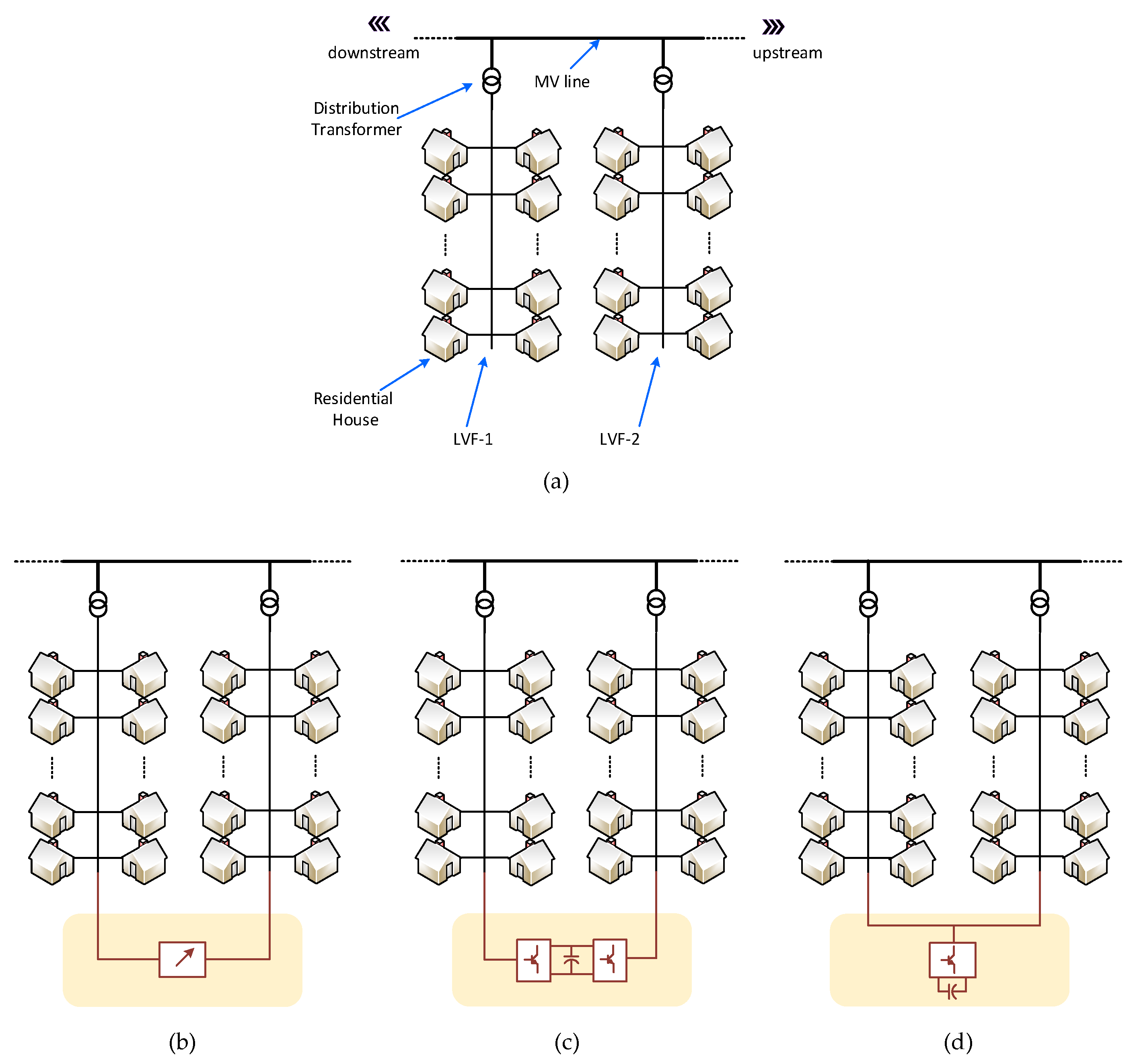
2. System under Consideration

Let us consider the MV line in Figure 1a that supplies two LVFs, namely LVF-1 and LVF-2, through two distribution transformers. The MV line is assumed to be a three-phase, three-wire system while each LVF is a three-phase, four-wire, mutual-earthed neutral (MEN)-type network [50]. Each distribution transformer is assumed to be a three-phase Dyn type. This is a common practice in Australia and the majority of Asian, European, and African countries but is not common in North America [1]. In Australia, the LVFs are usually supplied by a 25–315 kVA three-phase distribution transformer and are usually about 400 m long [50,51].
Figure 1d illustrates the considered system of coupled LVFs in this research. It is to be noted that although the coupled LVFs in Figure 1d are supplied by the same MV line, all provided discussions in this paper are general and thus valid and applicable even if they are supplied from different MV lines.
The DSTATCOM, installed at the coupling point of neighboring LVFs, is composed of a capacitor-based neutral-clamped dc link, a three-phase, three-leg VSC composed of insulated gate bipolar transistors (IGBTs) and anti-parallel diodes, and proper LC-type output passive filters [33]. The structure and control principle of the DSTATCOM is given in Appendix A.
Each radial LVF is protected against the short-circuit faults in the LVF by a switch-fuse (SF) at the secondary side of the distribution transformer, namely SF-1 and SF-2 [51]. Each SF has backup protection, which is a cut-out fuse at the primary side of the distribution transformer. The cut-out fuse also protects the distribution transformers in case of traveling surges (from switching or lightning) in the MV line.
Before discussing the protection schemes for the network in Figure 1d, let us consider the network in Figure 1b, which is the same as the system in Figure 1d if the DSTATCOM is ignored. The short-circuit fault conditions and the protection scheme will be discussed for this system first. Then, it will be modified for the system in Figure 1d to consider the presence of a DSTATCOM at the coupling point of the LVFs.
In the system in Figure 1b, depending on the PVs generation and load demand, a bidirectional current can flow in either of the LVFs in normal conditions; however, during short-circuit faults, a current will flow from the upstream side of all LVFs (i.e., the corresponding MV lines) to the fault point. In the rest of this section, first, the fault current contribution of each LVF for a short-circuit fault in one of the LVFs is investigated. Then, based on the findings of this investigation, the proper protection scheme is investigated for this system.

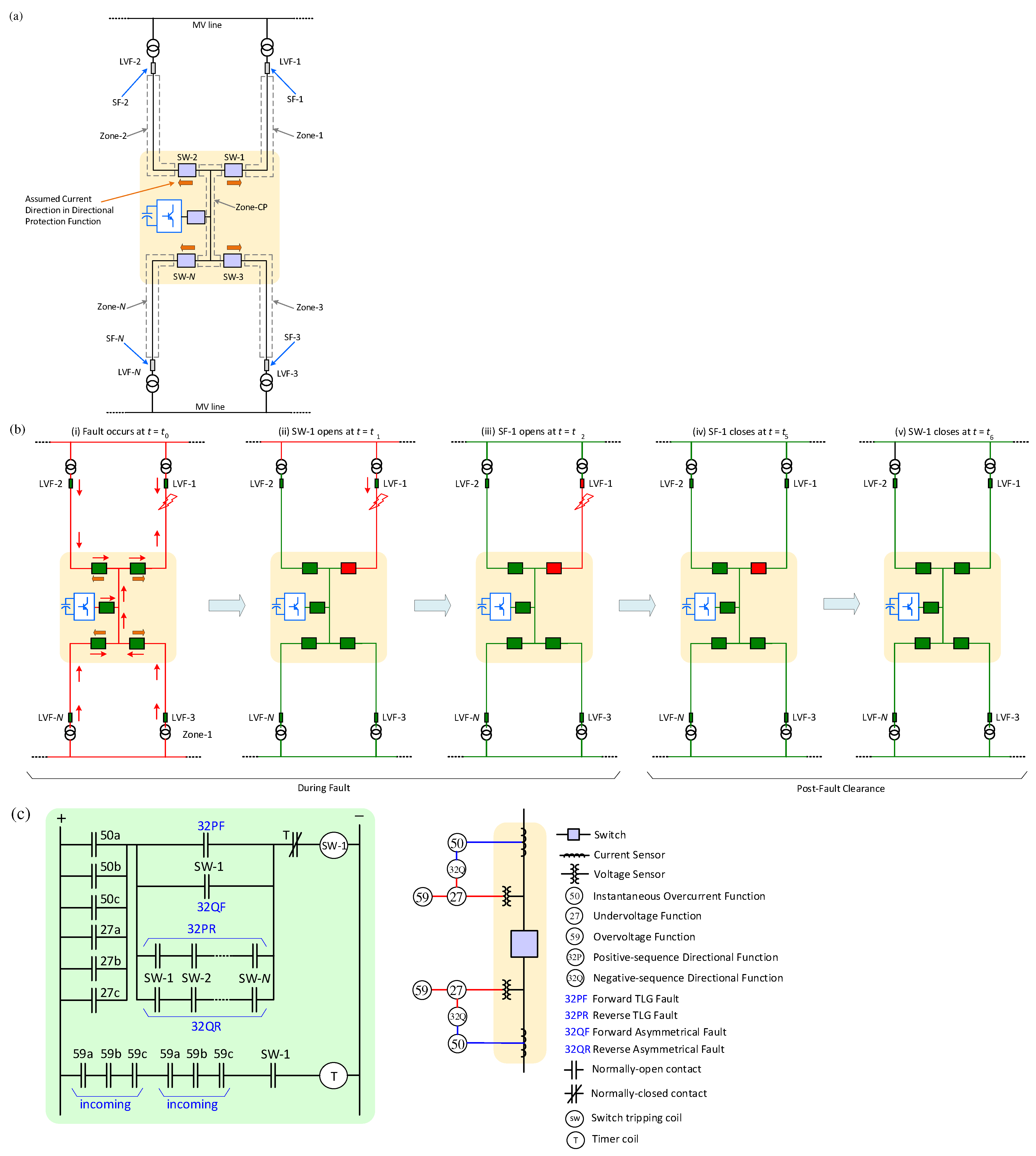
3. Desired Operation of the System of Coupled LVFs under Fault Conditions

As discussed above, a bidirectional power flow can be observed in either of the LVFs and through the switch in the system in Figure 1b and in normal conditions, as shown in Figure 2a. This figure also illustrates the protection zones of the system. Following the occurrence of a short-circuit fault in either of the LVFs, current flows from the upstream side of both LVFs towards the fault point, as shown in Figure 2b(i). It is desired to isolate the coupled LVFs immediately after fault occurrence with the help of the switch, which is located at the coupling point of the LVFs, as shown in Figure 2b(ii). It is to be noted that the switch can be a mechanical or a power electronics-based type (see Appendix B).
Appendix C discusses the analytical approach to calculate the short-circuit current under various fault types. If the switch isolates the LVFs, the fault current will be only supplied from the faulted LVF side (i.e., LVF-1) until SF-1 isolates the fault, as shown in Figure 2b(iii). However, if the switch fails to isolate the LVFs in time, both SF-1 and SF-2 will see the fault and both LVFs will be tripped, as shown in Figure 2c(ii,iii), which is an undesirable consequence of switch failure. A proper protection scheme for the switch, as well as the required settings, are discussed below:
Following a short-circuit fault in either of the LVFs, a portion of the short-circuit fault flows through the switch. Thus, the opening operation of this switch can be based on an overcurrent protection function, otherwise popularly known as the ‘phase 50′ function (see Figure 2d). In this case, the current pickup level (IP) for the overcurrent function needs to be higher (i.e., 1.1–1.25 times larger) than the largest nominal current of both distribution transformers [52], i.e.,
I P = ( 1.1 1.25 ) × max ( S T 1 , S T 2 ) 3 V LVF
where VLVF is the nominal line-line voltage of the LVFs (e.g., 380, 400, or 415 Vrms based on the different nominal voltages of different countries), S T 1 and S T 2 are assumed to be the ratings of the distribution transformers in LVF-1 and LVF-2, respectively, and max(.) represents the maximum function. Thus, the switch will not cause nuisance tripping when one of the distribution transformers supplies both feeders (under emergency or maintenance periods). On the other hand, the time multiplier setting (TMS) of the overcurrent protection function should be designed such that for a fault in either of the LVFs, the switch trips before SF-1 and SF-2. Otherwise, undesirable tripping will occur if SF-2 trips LVF-2 faster than the switch.
If the fault contribution of the healthy LVF (i.e., LVF-2) is smaller than IP (which can happen due to the fault type/location/impedance or the impedance of the LVFs or distribution transformers), the overcurrent protection will fail to open the switch. To avoid such issues, another protection function can be used in parallel with the overcurrent protection function.
Since during a short-circuit fault in either of the LVFs, the voltage rms in the faulted phase(s) drops all along both LVFs, an undervoltage protection function, otherwise popularly known as the ‘phase 27′ function, can be utilized as a backup protection function to the overcurrent protection function. Let us define VP (e.g., 0.6 pu) as the pickup level for the undervoltage protection function. The undervoltage protection function will be coordinated to open the switch if the voltage rms on both sides of the switch drops below VP. Thereby, the switch will open as soon as either of the overcurrent or undervoltage functions flags a fault. Note that the protection approach has to be applied for each phase of the system and the switch needs to open after a fault flag is issued from either of the phases. This is illustrated in the ladder diagram in Figure 2d.
Based on the above discussion, the desired sequence of the operation of the protective devices should be defined as discussed below:
  • Fault occurs at t = t0;
  • Action-1: The switch at the coupling point of the LVFs trips at t = t1 (based on the command of the overcurrent and/or undervoltage functions);
  • Action-2: The SF at the secondary side of the distribution transformer of the faulted LVF (i.e., SF-1) trips at t = t2;
  • Action-3: The SF at the secondary side of the distribution transformer of the non-faulted LVF (i.e., SF-2) trips at t = t2′ as backup protection when action-1 fails;
  • Action-4: The cut-out fuse at the primary side of the distribution transformer of the faulted LVF trips at t = t3 as a backup protection when action-2 fails;
  • Action-5: The cut-out fuse at the primary side of the distribution transformer of the non-faulted LVF trips at t = t3′ as a backup protection when action-3 fails;
  • Action-6: The first protective device in the MV line trips at t = t4 when either action 4 or 5 fails;
in which t0 < t1 < t2 < t3 < t4 and t0 < t1 < t2′ < t3′ < t4. Note that t2 may be equal, larger, or smaller than t2′. Similarly, t3 may be equal, larger, or smaller than t3′; however, t3′ > t2 and t3 > t2′. The difference between t2 and t2′ as well as the difference between t3 and t3′ depends on the portion of the fault current passing through the SFs and cut-out fuses of the LVFs. Such coordination will be achieved by applying proper TMS for the overcurrent function and coordinating it with the time-current characteristics of SF-1 and SF-2 as well as by applying a proper delay-time for the undervoltage protection function. This is illustrated schematically in Figure 3.
After fault clearance, the SF will close and will energize LVF-1, as shown in Figure 2b(iv). Let us assume it happens at t = t5 (where t5 may be much larger than t4 in case of non-transient faults). The switch is still at the open status. The voltage rms in all phases on both sides of the switch will be restored to the acceptable limits at t = t5′ (where t5′ > t5). At this condition, the protection scheme can initiate a command for the switch to close, as shown in Figure 2b(v). This will occur at t = t6, where t6 = t5 + ΔT1 (i.e., after a fixed delay time of a few seconds or minutes). An overvoltage function, otherwise, popularly known as the ‘phase 59’ function, with a voltage pickup of VP’ (e.g., 0.9 pu) can be used for this purpose. This is also illustrated in the ladder diagram in Figure 2d. In this figure, the switch will open when its tripping coil is energized and will close as soon as it is de-energized.

4. Operation of the System of Coupled LVFs in the Presence of a DSTATCOM

The discussions of Section 3 are focused on the system of coupled LVFs without a DSTATCOM (Figure 1b). The protection system will be more complex when a DSTATCOM is installed at the coupling point of the LVFs (Figure 1d) [47,48,49]. The main reason is that due to the presence of a DSTATCOM and its connection with multiple LVFs, a multi-switch scheme is required in which a switch is installed between the end node of each LVF and the DSTATCOM. Appendix D presents the analytical approach to calculate the short-circuit current under various fault types in the presence of a DSTATCOM.
Figure 4a illustrates a system of N-coupled LVFs where N ≥ 2. This system has N + 1 protection zones (i.e., one protection zone for each LVF and one protection zone for the coupling point), as illustrated in the figure. Similar to the discussions of Section 3, it is desired that following a short-circuit fault, only the faulted LVF gets isolated while the DSTATCOM is desired to remain connected to the non-faulted LVFs (see Figure 4b for desired performance of the system under a short-circuit fault in LVF-1).
Immediately after fault occurrence, current flows from the MV line(s) towards the fault point in all LVFs. In addition, current will flow from the dc link of the DSTATCOM toward the fault point. An important issue to be considered in such a case is that since the DSTATCOM is supplied by a dc capacitor, its stored energy is limited and it will discharge immediately after fault-occurrence (e.g., in less than 2 cycles); thereafter no current will be supplied by the DSTATCOM and the system will resemble the system in Figure 2a, with the only dissimilarity of higher number of coupled LVFs. It is to be noted that if the DSTATCOM has low-voltage ride-through capability or if it is supplied by an energy storage system such as a battery instead of a dc capacitor, it will continue to feed the fault for a longer period. However, the DSTATCOM proposed in [33] is composed of a dc capacitor to reduce the costs while providing the same system performance under normal conditions.
If the previously described overcurrent and undervoltage protection functions (in Figure 2d) are utilized for the switches, they will all sense the fault current and will sense the same voltage drop; thus, they will all trip (almost simultaneously or with a small difference in time) after a fault in either of the LVFs. Thereby, the DSTATCOM will also get isolated undesirably. To prevent this, a directional protection function is suggested.
Let us consider the assumed current directions for each switch as shown in Figure 4a, which is from the coupling point of the LVFs towards the distribution transformers. Once either of the overcurrent or undervoltage functions detects a short-circuit fault, it will also check the direction of the fault current. The switch which detects a forward fault will open but the switches that detect a reverse fault will remain closed. In Figure 4b(i), after a short-circuit fault in LVF-1, a forward fault is detected for SW-1 while a reverse fault is observed for the other switches (i.e., SW-2, 3, …, N). Thus, it is expected that only SW-1 will open while the other switches and the DSTATCOM will remain closed, as shown in Figure 4b(ii). Similar to the discussions of Section 3, this will be followed by the opening of SF-1 to trip LVF-1, as shown in Figure 4b(iii). In addition, after fault clearance, first SF-1 will close and will energize LVF-1, after which the overvoltage protection functions will detect acceptable voltage rms on both sides of SW-1 and it will close with a delay of ΔT1. The ladder diagram of this scheme is shown in Figure 4c for Switch-1. A similar ladder diagram will be utilized for all switches.
Detecting the forward or reverse fault can be achieved through different techniques [52]. It can be detected by comparing the angle difference between the current and the voltage as well as the direction of active power or reactive power. Alternatively, the sequence components can be used for the detection [53].
Positive-sequence voltage and current are the only sequence quantities that are present for a TLG fault. These quantities can be used to produce a single three-phase directional element to detect the fault direction in case of a TLG fault (see Appendix E). For this, the positive-sequence directional element torque, otherwise popularly known as the ‘T32P’ function, can be defined as [54]
τ T 32 P = | V po | | I po | cos V po ( I po + Z po )
where Vpo and Ipo, respectively, show the positive-sequence component of the voltage and current at the switch, and Zpo is the positive-sequence impedance of the line while |x| and ∠x, respectively, represent the absolute and angle of x. In (2), the positive torque represents a forward TLG fault while the negative torque represents a reverse TLG fault. In the ladder diagram in Figure 4c, for a forward TLG fault, the T32PF contact will close while for a reverse TLG fault, the T32PR will close. As can be seen from this figure, the T32P function is supervised by phase 50 and phase 27 protection functions.
For asymmetrical LG, LL, and DLG faults, (2) may lead to erroneous results in the fault direction discrimination. Thus, another approach will be used for the detection of the direction of such faults that is based on the negative-sequence impedance. For this, first, the negative-sequence component of voltage at the coupling point, denoted by V CP , and the negative-sequence component of current passing through switch-m, denoted by I sw - m , should be calculated. The negative-sequence impedance for switch-m, denoted by Z sw - m , can then be calculated as [55]
Z sw - m = V CP I sw - m m { 1,2 , N }
The following important points should be considered in this regard [53]:
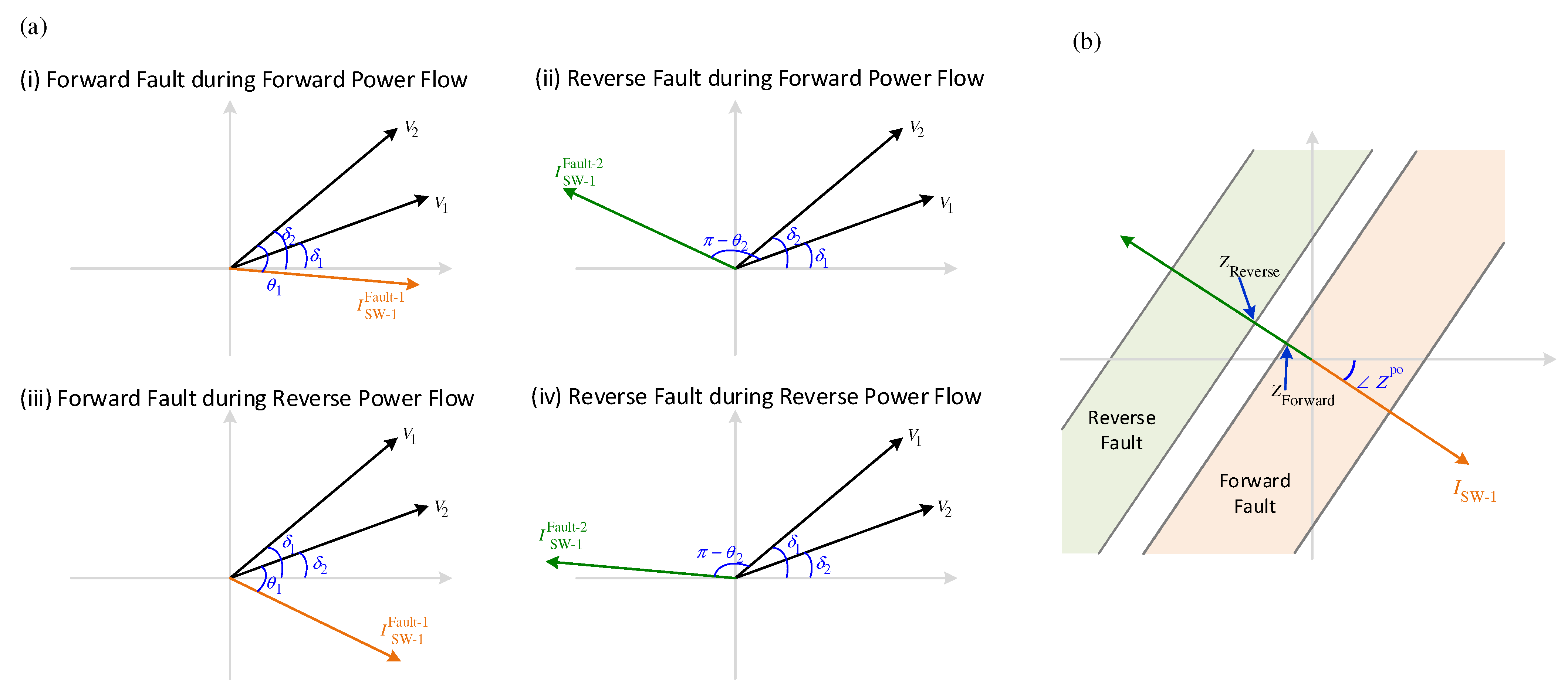
  • For both forward and reverse asymmetrical faults, V CP is always negative;
  • For a forward asymmetrical fault for switch-m, I sw - m lags the driving voltage by the characteristic angle of the line and is considered positive;
  • For a reverse asymmetrical fault for switch-m, I sw - m is in the reverse direction (180° phase shift) of the forward fault; and
  • For a forward asymmetrical fault, Z sw - m is always negative and for a reverse asymmetrical fault, Z sw - m is always positive.
In the ladder diagram in Figure 4c, for a forward asymmetrical fault, the T32QF contact will close while for a reverse asymmetrical fault, the T32QR will close. Similar to the T32P function, the T32Q function is also supervised by phase 50 and phase 27 protection functions. Alternatively, another suitable directional protection scheme such as those presented in [37,56,57,58,59] can be utilized.
The above discussions have focused on short-circuit faults in one of the coupled LVFs. On the other hand, a short-circuit fault may also occur on the coupling point of the LVFs (i.e., the connection point of the DSTATCOM). This fault will be detected as a reverse fault by all switches (i.e., either the T32PR or T32QR contact will close for all switches). This can be detected by a switch assuming a proper POTT is received from the T32PR and T32QR functions of all switches (as seen in Figure 4c). Under such conditions, it is desired that all LVFs isolate from each other in addition to the isolation of the DSTATCOM from the coupling point.
As discussed at the beginning of this section, the energy stored in the dc link of the DSTATCOM will discharge in a few cycles after a fault in either of the LVFs. This is valid for all fault types. Quicker fault detection by the protection scheme and operation of SW-1 will prevent a full discharge of the dc link. The DSTATCOM dynamic controller will facilitate the dc link voltage restoration after the opening of SW-1 (regardless of the level of discharge). Thus, a different protection scheme is developed for the switch located between the DSTATCOM and the coupling point of the LVFs. This switch is expected to isolate the DSTATCOM from the coupling point of the LVFs only based on a significant and sustained voltage deviation on the coupling point that can be detected by undervoltage/overvoltage protection functions with voltage pickups of 1.2 and 0.6 pu and after a time delay of ΔT2 where ( T 2 < T 1 ). It is to be noted that this switch is not expected to respond to short-circuit faults in either of the LVFs unless a significant and sustained voltage deviation is observed due to a fault (which is possible in the case of high-impedance faults).

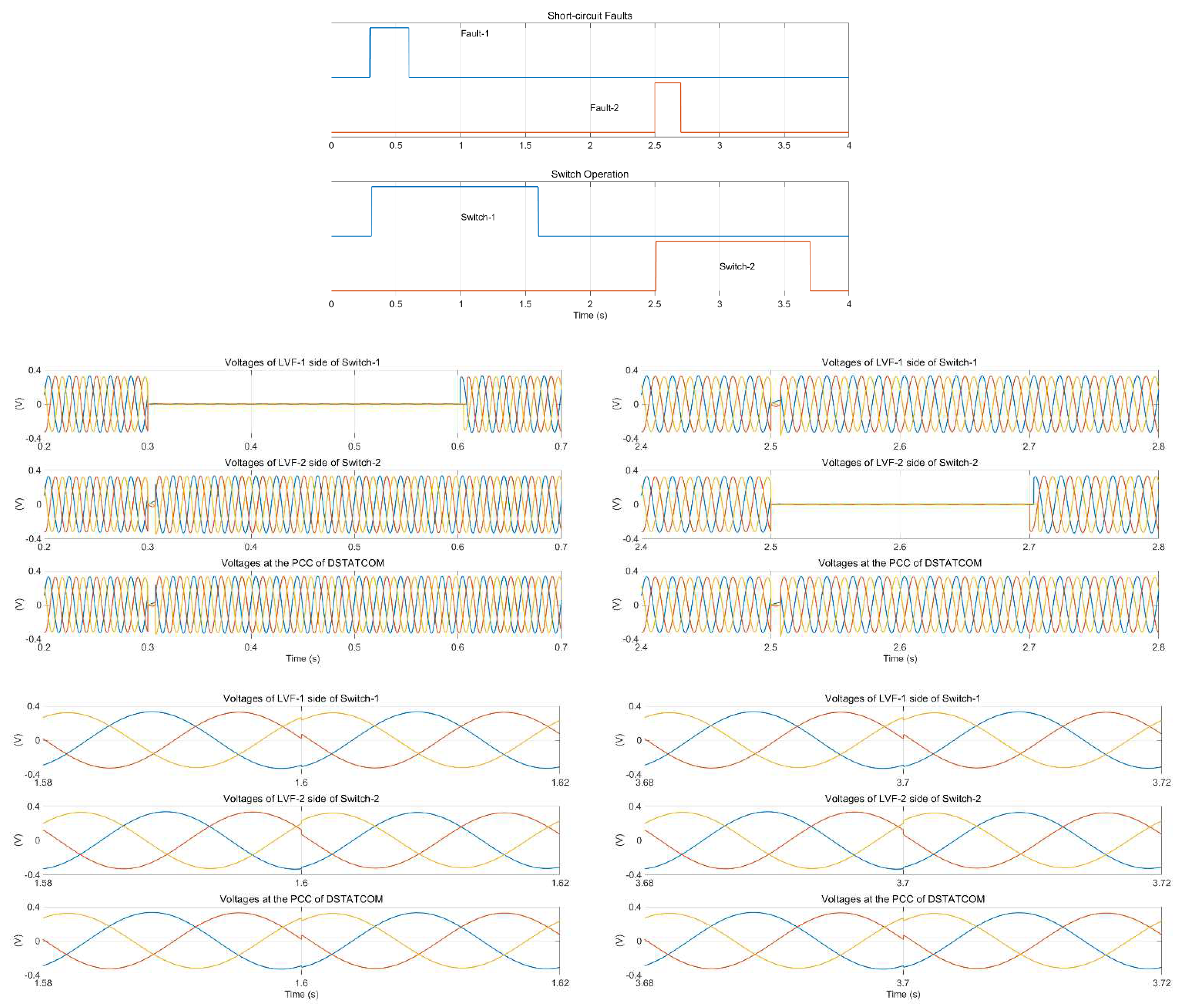
5. Case Studies and Simulation Results

As an example, assuming that the MV line in Figure 1b has a line-line voltage of 11 kV rms and a short-circuit fault capacity of 95 MVAsc, a number of contingency conditions are evaluated.
To evaluate the dynamic feasibility of the discussed protection approach for the system of coupled LVFs, several study cases are considered, a few of which are discussed below. The proposals are validated in PSCAD/EMTDC.
Let us consider an 11 kV MV line supplying two 11 kV/415 V Dyn-type distribution transformers, as illustrated schematically in Figure 1a. Only two radial three-phase, four-wire, MEN-type residential LVFs, namely LVF-1 and LVF-2, are considered in detail [60,61]. Each LVF is supplied by a distribution transformer with a rating of 200 kVA. The length of each LVF is taken as 400 m. The poles of each LVF are assumed to be located 40 m from each other. The feeders and their cross-sections are designed based on the nominal supplied power and the maximum acceptable voltage drop. The network data are for a typical LV urban residential network in Brisbane, Australia and are given in Appendix F. The residential loads are assumed to be in the range of 1–5 kW and are modeled as constant impedance type. The rooftop PV cells and inverters are modeled as discussed in [36]. The PV inverters are assumed to have a nominal rating of 1–5 kW and all are assumed to operate in unity.
First, let us consider the network in Figure 2a in which two LVFs are coupled through a single switch. The network is assumed to be initially at a steady-state condition. Two transient three-phase-to-ground faults, with a fault impedance of 1 mΩ, are later applied in the system. Fault-1 is applied in LVF-1 at t = 0.3 s and clears after 0.3 s while Fault-2 is applied in LVF-2 at t = 2.5 s and clears after 0.2 s. In both cases, the faults are detected within 0.01 s after fault-occurrence by the proposed approach; thus, the switch is opened in 0.01 s after both faults. The switch closes with a 0.5 s delay after the voltages on both sides of the switch return to the normal acceptable limit (i.e., after fault clearance). The results of this simulation are shown in Figure 5. This figure illustrates each fault and its duration, the open/close status of the switch at the period of study (i.e., 0 ≤ t ≤ 4), the three-phase voltages at either side of the switch, and the current flowing through the switch before fault-occurrence (i.e., t < 0.3 and 1.6 < t < 2.5), between fault-occurrence and opening of the switch (i.e., 0.3 ≤ t ≤ 0.31 and 2.5 ≤ t ≤ 2.51), after the switch is opened (i.e., 0.31 < t < 1.6 and 2.51 < t < 3.7) and at the switch closing time (i.e., t = 1.6 and t = 3.7). The results verify the appropriate operation of the switch (i.e., opening after detecting a short-circuit fault in either of the LVFs and closing after detecting the voltage restoration after fault clearance).
Now, let us consider the network in Figure 4a in which two LVFs are coupled through two switches. The network is assumed to be initially at steady-state condition. The same faults as discussed above are applied in this system. Similar to the previous case, the faults are detected within 0.01 s after fault-occurrence by the proposed approach. After Fault-1 (which occurs at t = 0.3 s on LVF-1), the negative-sequence impedance becomes negative and both switches detect a forward fault. Thus, only Switch-1 operates and disconnects the faulted LVF from the point of common coupling (PCC) of the DSTATCOM while Switch-2 remains closed. After Fault-2 (which occurs at t = 2.5 s on LVF-2), the negative-sequence impedance becomes positive and both switches detect a reverse fault. Thereby, only Switch-2 opens and the faulted LVF becomes isolated from the PCC of the DSTATCOM while Switch-1 remains closed. After fault clearance, the operated switch closes after the voltage restoration by a 0.5 s delay. The results of this simulation are shown in Figure 6. This figure illustrates each fault and its duration, the open/close status of each switch at the period of study, the three-phase voltages at the LVF-1 side of Switch-1, at the LVF-2 side of Switch-2 and at the PCC of the DSTATCOM before fault-occurrence, between fault-occurrence and opening of the appropriate switch, after the switch is opened, and at the switch closing time. The results verify the appropriate operation of the switches (i.e., the correct opening of the switch after detecting a short-circuit fault in the LVFs and its closing after detecting the voltage restoration after fault clearance).
It is to be noted that to focus more on the discussed protection approach and considering the fact that DSTATCOM operation and control is beyond the scope of this research, the DSTATCOM operation is not shown here.

6. Conclusions

The concept of coupling the neighboring LVFs is proposed in the literature as a technique for addressing the voltage drop and voltage rise problems of LVFs. This paper has focused on and proposed the protection for such a coupled LVF system when a short-circuit fault occurs in either of the LVFs. Through studies on an 11 kV network that supplies two neighboring LVFs via two separate distribution transformers and real network modeling, it is shown that overcurrent or undervoltage protection approaches are inadequate. Instead, the studies have demonstrated that a negative-sequence impedance-based directional overcurrent protection scheme can effectively and promptly discriminate the fault and properly protect the network by opening the corresponding switches. Through dynamic studies, the feasibility of the proposals for discriminating the fault is demonstrated for the considered system of coupled LVFs during short-circuit faults at various sections of the system. The studies have demonstrated that regardless of the fault location in the system of coupled LVFs, the developed proposal detected the faults within 0.01 s after fault occurrence, and thus, the corresponding switches open. Also, the studies illustrate that the corresponding switches close by the developed proposal within 0.5 s after the voltages on both sides of the switch return to the normal acceptable limit post fault clearance.

Funding

This research received no external funding.

Data Availability Statement

Data is unavailable due to privacy restrictions.

Conflicts of Interest

The author declares no conflict of interest.

Appendix A. Structure and Control of the DSTATCOM

The considered DSTATCOM is a transformer-less, neutral-clamped, three-phase, three-leg VSC with IGBTs along with anti-parallel diodes and snubber circuits (see Figure A1) [33]. The dc link is composed of two identical series-connected dc capacitors. A neutral-claimed dc link is considered to provide a circulation path for the zero-sequence component of the current. Each VSC is connected to the LVF through an Lf-Cf filter to suppress the ripples of the current and to bypass the switching harmonics of the voltage. The resistance Rf represents the switching power losses of the VSC [61].
Figure A1. DSTATCOM is installed at the coupling point of the LVFs with its per-phase closed-loop controller.
Energies 16 06009 g0a1
The first responsibility of the DSTATCOM in this application is to guarantee a desired balanced voltage at the coupling point while its other responsibility is to facilitate active power circulation among the phases of one LVF. To realize these tasks, the Vdc of the DSTATCOM is regulated to a constant desired level of V dc r e f with minimum ripples. Vdc will fluctuate if the dc link exchanges active power with the coupling point; hence, the VSC modifies its switching to prevent the exchange of active power between the coupling point and VSC [61]. The active power exchange can be controlled by regulating the angle of the voltage at the coupling point of VSC. Thereby, the angle of the voltage across capacitor Cf of VSC (δ) is modified based on the variations of the dc link voltage using a proportional-integrator (PI) controller, as [62]
δ = k P ( V dc r e f ) 2 V dc 2 + k I ( V dc ref ) 2 V dc 2 d t
where kP and kI are the parameters of the PI controller. δ, which is calculated from (A1), is applied as the desired angle for the voltage across the capacitor Cf connected to phase a while its 120° phase shifts will be applied as the desired angle for the voltage across the capacitor Cf connected to phase b and c. On the other hand, the VSC needs to be controlled such that a desired voltage magnitude (|V|ref) appears at the PCC.
Based on the above discussions, a voltage-controlled technique is deployed for the control of VSC. The desired time-domain voltage references across the capacitors Cf of the VSC in the DSTATCOM system are
v a ref t = 2 V r e f sin ( ω t + δ ) v b ref t = 2 V r e f sin ( ω t + δ 120 ° ) v c ref t = 2 V r e f sin ( ω t + δ + 120 ° )
where δ is calculated from (A1), |V|ref is assumed to be 1 pu and ω = 2πf where f is the nominal frequency. Equation (A2) guarantees that a balanced three-phase voltage will appears at the coupling point of the DSTATCOM. Since the derived voltage references are time-variant, a per-phase (abc) control technique is developed and used in this research. A linear quadratic regulator (LQR)-based state feedback control [63] is used in this research, which is discussed in detail in [33]. The block diagram of the closed-loop control system is shown for one phase of the VSC and filter system in Figure A1. The above technique is a per-phase control technique; hence, in a similar fashion, the IGBTs’ turn on/off will be determined for the other two legs (i.e., the other two phases) of the DSTATCOM system.
Alternatively, the DSTATCOM with the same structure but with a different control objective can be utilized in which the DSTATCOM operates in current control mode when the voltage rms at the coupling point of the LVFs is within desirable limits but operates in the proposed voltage control mode when the voltage rms exceeds the desirable limits, as suggested in [64].

Appendix B. Structure of the Coupling Point Switch

The switch installed at the coupling point of the LVFs can be a mechanical or a power electronics-based type. LV switch disconnectors or load break switches are commercially available in the market (with a nominal operational current capacity in the range of a few amperes to a few kilo amperes and with a rated breaking capacity of a few tens of kilo ampere) [65]. A switch with the same mechanical current tripping structure but operated with the proposed protection scheme can be used. Alternatively, power electronics-based switches, with any of the topologies shown in Figure A2 can be utilized [66]. It is to be noted that Figure A2 illustrates the structures for one phase only. In this figure, structure i is composed of anti-parallel thyristors while structure ii is composed of anti-parallel IGBTs. In both structures, each of the anti-parallel power electronic devices (i.e., the IGBT or thyristor) conducts only half a cycle in each cycle. Structure ii has the advantage of being fully controlled (controlled turn-on and turn-off) while structure i is a half-controlled type (i.e., a controlled turn-on while a commutation-based turn-off). Both structures need a switching control scheme for the power electronic devices. Structure iii is composed of a diode bridge with an IGBT inside. In this structure, a pair of diodes conduct in each half cycle while the IGBT continuously conducts the current. The IGBT should open only when the proposed protection scheme detects a fault in the system. Thus, this structure has a much simpler switching control than structures i and ii. Therefore, it can be concluded that structure iii is superior to the other two structures, mainly from the simpler switching scheme perspective. Generally, two issues of cost and power loss can be the main factors when selecting either the mechanical or structure iii type power electronics-based switch, which both depend on the nominal current of the switch.
Figure A2. Three power electronics-based topologies are usable as the switch between the end of each coupled LVF and the DSTATCOM.
Energies 16 06009 g0a2

Appendix C. Short-Circuit Studies for the System of Coupled LVFs without a DSTATCOM

Let us consider the system in Figure 1b. Let us assume that a short-circuit fault occurs in one of the LVFs (e.g., LVF-1). Immediately after fault-occurrence, currents will flow in both LVFs from the MV line towards the fault point (see Figure 2b(i)). Single line-to-ground (SLG), line-to-line (LL), double line-to-ground (DLG), and triple line-to-ground (TLG) faults are considered. Immediately before the fault, phase-a voltages at the primary side of each distribution transformer are assumed to be V T 1 and V T 2 . Additionally, Z T 1 and Z T 2 are, respectively, the per-phase leakage impedances of the distribution transformers in LVF-1 and LVF-2. Moreover, it is assumed that the fault has an impedance of ZFault and occurs at k % of the feeder length from its beginning (where 0 ≤ k ≤ 100). Thus, the system in Figure 2b(i) can be represented as Figure A3a.
It is to be noted that except for the TLG fault, Fortescue’s positive, negative, and zero-sequence components will be used for the asymmetrical SLG, LL, and DLG short-circuit studies [67]. Thus, the sequence components of the impedances are also required. Dyn-type distribution transformers, considered in this research, have equal positive-, negative-, and zero-sequence impedances (which are also equal to the per-phase leakage impedance of the transformer).
The considered three-phase, four-wire LVFs in this research are assumed to have a horizontal ABCN configuration [50], as shown in Figure A3b(i). The equivalent impedance of this LVF between two buses can be illustrated schematically in Figure A3b(ii) where each of these impedances is calculated using modified Carson’s equations [68] in a 50 Hz system from
z u u = r u + 0.04934 + j 0.062832 7.10988 Ln G M R u z u v = 0.04934 + j 0.062832 [ 7.10988 Ln ( D u v ) ]
where u  { a , b , c , n } , v  { a , b , c , n } , zuu is the self-impedance of conductor u (in Ω/km), z u v is the mutual impedance between conductors u and v (in Ω/km), ru is the ac resistance of conductor u (in Ω/km), G M R u is the geometric mean radius of conductor u (in cm), D u v is the distance between conductors u and v (in cm), L n ( . ) represents the natural logarithm function, and j 2 = 1 . Hence, (A3) considers the non-transposed characteristics of the conductors, image conductors below ground, and network configuration. From (A3), the total impedance of the three-phase, four-wire LVF between two buses in phase quantities, denoted by [ Z LVF abcn ] , can be described as
[ Z LVF abcn ] = z aa z ab z ac z an z ba z bb z bc z bn z ca z cb z cc z cn z na z nb z nc z nn
Figure A3. (a) Equivalent impedance network in Figure 2a during a short-circuit fault in LVF-1, (b) Considered LVF structure and its equivalent impedance between adjacent buses, (c) Equivalent sequence impedance networks during asymmetrical short-circuit faults in LVF-1.
Energies 16 06009 g0a3
Using Kron reduction, this impedance can be rewritten in its equivalent 3 × 3 dimension as [68,69]
[ Z LVF abc ] = z aa - n z ab - n z ac - n z ba - n z bb - n z bc - n z ca - n z cb - n z cc - n = z aa z nn z an z na z ab z nn z an z nb z ac z nn z an z nc z ba z nn z bn z na z bb z nn z bn z nb z bc z nn z bn z nc z ca z nn z cn z na z cb z nn z cn z nb z cc z nn z cn z nc
From (A5), the LVF impedance in sequence components, denoted by Z LVF zpn , can be calculated from
Z LVF zpn = A ] 1 Z LVF abc ] A = z ze - ze z ze - po z ze - ne z po - ze z po - po z po - ne z ne - ze z ne - po z ne - ne
where
A = 1 1 1 1 a 2 a 1 a a 2                 a = 1 + i 3 / 2
Equation (A6) can be simplified to [67,69]
Z LVF zpn = z ze - ze 0 0 0 z po - po 0 0 0 z ne - ne
where
z ze - ze = z S + 2 z M z po - po = z ne - ne = z S z M z S = z aa - n = z bb - n = z cc - n z M = z ab - n = z ac - n = z ba - n = z bc - n = z ca - n = z cb - n
if all phase conductors have the same cross-sections (i.e., the same self-impedance) and the same distance from each other (i.e., the same mutual-impedance). However, neglecting the difference of up to 3–4% among z aa - n , z bb - n , and z cc - n and among z ab - n = z ba - n , z ac - n = z ca - n , and z bc - n = z cb - n in the rest of this study, (A7) is utilized as the sequence impedance of the LVFs, which significantly simplifies the computation burden without impacting the results. It is to be noted that in the rest of this section, zpo-po, zne-ne, and zze-ze are, respectively, represented by ( z LVF ) po , ( z LVF ) ne , and ( z LVF ) ze while the impedances of LVF-1 and LVF-2 are denoted by Z LVF 1 and Z LVF 2 .

Appendix C.1. Triple Line to Ground (TLG) Short-Circuit Faults

Considering the fact that the residential loads and rooftop PVs in the system in Figure A3a have single-phase connections and do not observe equal consumption/generation for all phases of a specific node at every instant of time, the system in Figure A3a is considered an unbalanced system for load flow studies. However, since the fault current is much larger than the load current and assuming that the per-phase impedance of each phase of an LVF is the same, the system in Figure A3a can be considered a balanced system for TLG faults. Immediately after fault-occurrence, currents will flow in each phase of LVF-1 and LVF-2 from the corresponding MV line towards the fault point. Let us denote the current in phase a of LVF-1 and LVF-2 by I Fault ph - a LVF - 1 and I Fault ph - a LVF - 2 . These currents are
I Fault ph - a LVF - 1 = V T 1 V Fault Z T 1 + k Z LVF 1 I Fault ph - a LVF - 2 = V T 2 V Fault Z T 2 + Z LVF 2 + 1 k Z LVF 1
where V Fault is the voltage in phase a of the faulted LVF at the fault point and is equal to
V Fault ph - a = Z Fault I Fault ph - a
while I Fault ph - a = I Fault ph - a LVF - 1 + I Fault ph - a LVF - 2 . It is noteworthy that I Fault ph - a = I Fault ph - b = I Fault ph - c for a TLG fault on the balanced system in Figure A3a. It is to be reminded that for the same fault in LVF-1, prior to coupling the LVFs, the fault current would have been only I Fault LVF - 1 , which is now increased to I Fault LVF - 1 + I Fault LVF - 2 . Solving (A8) and (A9) and after some simplifications, one gets
I Fault ph - a LVF - 1 = α 2 V T 1 α 3 V T 2 / α 4 I Fault ph - a LVF - 2 = α 3 V T 1 + α 1 V T 2 / α 4 I Fault ph - a = α 2 α 3 V T 1 + α 1 α 3 V T 2 / α 4
where
α 1 = Z T 1 + k Z LVF 1 α 2 = Z T 2 + Z LVF 2 + 1 k Z LVF 1 α 3 = Z Fault α 4 = α 1 α 2 α 3 2
It is to be highlighted that (A10) describes the fault current assuming that the fault impedance dynamics are ignored. Furthermore, it is assumed that the voltages at the primary side of the distribution transformers are three-phase balanced voltages and are not affected by the fault. It is noteworthy that I Fault LVF - 1 might be larger than or equal to I Fault LVF - 2 depending on the fault location and the impedances of the LVFs and the distribution transformers.

Appendix C.2. Single Line to Ground (SLG) Short-Circuit Faults

Now, let us assume an SLG fault in phase a of LVF-1 in the system in Figure A3a. The positive-, negative-, and zero-sequence networks can be represented as shown in Figure A3c(i). Using the equivalent sequence network connections for an SLG, shown in this figure, the fault current in sequence components is given by
I Fault po = I Fault ne = I Fault ze = V eq po Z eq po + Z eq ne + Z eq ze + 3 Z Fault
where
Z eq po = Z eq ne = β 1 | | β 2 Z eq ze = β 3 | | β 4 V eq po = β 2 V 1 + β 1 V 2 β 1 + β 2 β 1 = Z T 1 + k ( Z LVF 1 ) po β 2 = Z T 2 + ( Z LVF 2 ) po + 1 k ( Z LVF 1 ) po β 3 = Z T 1 + k ( Z LVF 1 ) ze β 4 = Z T 2 + ( Z LVF 2 ) ze + 1 k ( Z LVF 1 ) ze
while x   | |   y = x × y / x + y . From (A11), the fault current observed in the faulted phase (i.e., phase a) can be calculated as
I Fault ph - a = 3 V eq po Z eq po + Z eq ne + Z eq ze + 3 Z Fault
The equivalent fault current flowing in LVF-1 and LVF-2 towards the fault point in sequence components, respectively denoted by I Fault u LVF - 1 and I Fault u LVF - 2 where u po ,   ne ,   ze , can then be explained as
I Fault po LVF - 1 = β 2 I Fault po Γ V / β 1 + β 2 I Fault ne LVF - 1 = β 2 I Fault ne / β 1 + β 2 I Fault ze LVF - 1 = β 4 I Fault ze / β 3 + β 4 I Fault po LVF - 2 = β 1 I Fault po + Γ V / β 1 + β 2 I Fault ne LVF - 2 = β 1 I Fault ne / β 1 + β 2 I Fault ze LVF - 2 = β 3 I Fault ze / β 3 + β 4
where Γ V = V T 1 V T 2 . Using (A13), the fault current contribution in phase a from each LVF can be calculated from
I Fault ph - a LVF - 1 = I Fault ze LVF - 1 + I Fault po LVF - 1 + I Fault ne LVF - 1 I Fault ph - a LVF - 2 = I Fault ze LVF - 2 + I Fault po LVF - 2 + I Fault ne LVF - 2

Appendix C.3. Line to Line (LL) Short-Circuit Faults

For an LL fault between phases b and c of LVF-1 in the system in Figure A3a, using the equivalent sequence network connections in Figure A3c(ii), the fault current in sequence components can be expressed as
I Fault po = V eq po Z eq po + Z eq ne + Z Fault I Fault ne = I Fault po I Fault ze = 0
From (A15), the fault current observed in phases b and c can be calculated as
I Fault ph - b = I Fault ph - c = a 2 a V eq po Z eq po + Z eq ne + Z Fault
It is to be noted that I Fault ph - b = I Fault ph - c while I Fault ph - b I Fault ph - c = ± 180 ° . The contribution of each LVF on the fault current can then be explained from (A13) in sequence components and then used to define them in phases b and c of each LVF from
I Fault ph - b LVF - f = I Fault ze LVF - f + a 2 I Fault po LVF - f + a I Fault ne LVF - f I Fault ph - c LVF - f = I Fault ze LVF - f + a I Fault po LVF - f + a 2 I Fault ne LVF - f           f 1 , 2

Appendix C.4. Double Line to Ground (DLG) Short-Circuit Faults

For a DLG fault among phases b, c, and ground in LVF-1 of the system in Figure A3a, using the equivalent sequence network connections in Figure A3c(iii), the fault current in sequence components can be expressed as
I Fault po = V eq po Z eq po + Z eq ne | | Z eq ze + 3 Z Fault I Fault ne = V eq po Z eq po I Fault po Z eq ne I Fault ze = I Fault po I Fault ne
which are then used to define the fault current in phases b and c from
I Fault ph - b = I Fault ze + a 2 I Fault po + a I Fault ne I Fault ph - c = I Fault ze + a I Fault po + a 2 I Fault ne
The contribution of each LVF on the fault current can then be explained from (A13) in sequence components and then used in (A17) to define them in phases b and c of each LVF.

Appendix D. Short-Circuit Studies for the System of Coupled LVFs in the Presence of a DSTATCOM

Let us consider the network in Figure 3a. It is assumed that before the fault, the voltages at the primary side of each distribution transformer in Figure 3a are V T 1 , V T 2 , , V T N . Immediately after fault-occurrence, I Fault LVF - 1 flows from the MV line towards the fault point in LVF-1 while N−1 currents, denoted by I Fault LVF - 2 , …, I Fault LVF - N , will flow in the LVFs from the MV line(s) towards the coupling point of the LVFs. These currents are
( I Fault LVF - 1 ) # = V T 1 V Fault # Z T 1 + k Z LVF 1 ( I Fault LVF - f ) # = V f V CP # Z T j + Z LVF j                     f 2 , , N
where notation # represents this condition. In addition, a current will flow from the dc link of the DSTATCOM toward the fault point. Let us denote this current by I DSC which can be expressed as
( I Fault DSC ) # = V DSC V CP # Z DSC
where ZDSC represents the equivalent impedance of the DSTATCOM. Thus, the equivalent current flowing from the coupling point of the LVFs towards the fault point, denoted by Ieq, can be expressed as
I eq # = ( I Fault DSC ) # + f = 2 N ( I Fault LVF - f ) # = V CP # V Fault # 1 k Z LVF 1
Thus, the fault current will be equal to I Fault # = I 1 # + I eq # .
As discussed in Section 4, the current supplied from the dc link of the DSTATCOM towards the fault point will result in a fast discharge of stored energy of the dc link which will lead to the reduction of the voltage of the dc link to zero and thus the failure of voltage regulation. In the rest of this section, the post-fault performance of the system (i.e., after the decay of the transients of the DSTATCOM) is discussed. Let us consider the system in Figure A4a with a TLG fault. The post-fault system can be expressed by
( I Fault LVF - 1 ) $ = V T 1 V Fault $ Z T 1 + k Z LVF 1 ( I Fault LVF - f ) $ = V f V CP $ Z T f + Z LVF f f 2 , , N I eq $ = f = 2 N ( I Fault LVF - f ) $ = V CP $ V Fault $ 1 k Z LVF 1 V Fault $ = Z Fault ( I Fault LVF - 1 ) $ + I eq $
where notation $ represents the post-fault condition. Solving (A23) and simplifying it, one can derive each current as
I LVF - 1 I LVF - 2 I LVF - f I LVF - N Fault $ = B N × N 1 . V 1 V 2 V f V N $
where
B = α 3 + Z T 1 + k Z LVF 1 O 1 × N 1 O N 1 × 1 1 k Z LVF 1 + diag Z T f + Z LVF f
while Ox×y is a matrix of zero elements with x rows and y columns, and diag Z T f + Z LVF f f ∈ {2, …, N} produces a square matrix with the size of N 1 with diagonal elements of Z T f + Z LVF f in which f is varied from 2 (in the first diagonal element) to N (in the last diagonal element). It is to be highlighted that similar to (A10), in (A24) the fault impedance dynamics are ignored and it is assumed that the voltages at the primary side of the distribution transformers are not affected by the fault.
From (A23), it can be said that I Fault LVF - 1 might be larger, smaller, or equal to I eq , depending on the fault location, the impedances of the LVFs and the distribution transformers, and the number of coupled LVFs.
Now, let us assume an SLG fault in phase a of LVF-1 in the system in Figure A4a with the sequence networks in Figure A4b. The fault current in sequence components can be calculated similarly to (A11) assuming that
( Z eq po ) $ = ( Z eq ne ) $ = β 1 $ | | β 2 $ ( Z eq ze ) $ = β 3 $ | | β 4 $ ( V eq po ) $ = β 2 $ V 1 + β 1 $ V 2 β 1 $ + β 2 $ ) β 1 $ = Z T 1 + k ( Z LVF 1 ) po β 2 $ = 1 k ( Z LVF 1 ) po + Z T 2 + ( Z LVF 2 ) po Z T N + ( Z LVF N ) po β 3 $ = Z T 1 + k ( Z LVF 1 ) ze β 4 $ = 1 k ( Z LVF 1 ) ze + Z T 2 + ( Z LVF 2 ) ze Z T N + ( Z LVF N ) ze
For an LL fault between phases b and c as well as a DLG fault among phases b, c, and ground in LVF-1 of the system in Figure A4a, the fault current can be calculated similarly to the discussions in Equations (A22) and (A23). It is to be noted that when defining the contribution of each LVF on the fault current, a system of N-linear equations will be solved.
Figure A4. (a) Equivalent impedance network in Figure 3a during a short-circuit fault in LVF-1, (b) Equivalent sequence impedance networks during asymmetrical short-circuit faults in LVF-1.
Energies 16 06009 g0a4

Appendix E. Directional Protection Function and Its Settings

Let us consider the network in Figure 3a. For simplicity, let us assume this system is composed of N = 2 coupled LVFs, namely LVF-1 and LVF-2. Let us denote δ 1 = V T 1 ph - a , δ 2 = V T 2 ph - a . It can be said that δ 2 > δ 1 when power flows from LVF-2 to LVF-1 (see phasor diagrams in Figure A5a(i,ii)) while δ 1 > δ 2 when it flows from LVF-1 to LVF-2 (see phasor diagrams in Figure A5a(iii,iv)). Two TLG faults, one in LVF-1, denoted by Fault-1, and one in LVF-2, denoted by Fault-2, will be investigated. In both cases, the post-fault current (i.e., the current after the decay of the transients) passing through SW-1 in phase a, denoted by ISW-1, will be investigated. The short-circuit studies of Appendix C.1 address the system performance during Fault-1 when ZFault ≠ 0. A similar analysis can be applied to Fault-2. However, for simplicity, let us assume that ZFault = 0. In addition, let us denote Z Fault LVF - 1 = Z Fault LVF - 1 θ 1 as the total per-phase impedance between V T 2 and the fault point for Fault-1. Similarly, let us denote Z Fault LVF - 2 = Z Fault LVF - 2 θ 2 as the total per-phase impedance between V T 1 and the fault point for Fault-2. Under such assumptions, the post-fault current of SW-1 in phase a can be expressed for Fault-1 and Fault-2 as
I SW - 1 Fault - 1 = V T 2 Z Fault LVF - 1 = V T 2 Z Fault LVF - 1 δ 2 θ 1 I SW - 1 Fault - 2 = V T 1 Z Fault LVF - 2 = V T 1 Z Fault LVF - 2 π + δ 1 θ 2
Thus, it can be seen that during a forward fault in an LVF (i.e., Fault-1), the fault current seen by SW-1 lags the corresponding voltage (i.e., V T 2 ) by θ1 (see Figure A5a(i,iii)). However, during a reverse fault (i.e., Fault-2), the current leads the corresponding voltage (i.e., V T 1 ) by 180°–θ2 (see Figure A5a(ii,iv)) [37]. It is to be noted that these are valid regardless of the power flow direction through the switch in the pre-fault conditions. The above discussions are expandable to a system of N-coupled LVFs as only one of the switches will detect a forward fault and all other switches will detect a reverse fault.
Directional protection functions are used to detect the direction of a fault [52]. They are used to control the overcurrent protection functions or to supervise distance protection functions. Directional relays use the concept of torque to detect a fault, which is achieved by using the phase shift between the voltage (of the faulted phase, healthy-phase, or pre-fault conditions [70]) and the faulted phase current. The torque can be derived for each phase but is usually derived in terms of sequence components. Different torques are used by manufacturers for directional protection functions [71,72,73]. A positive-sequence directional relay can be used for the detection of balanced TLG faults. However, the positive-sequence torque may fail to determine the direction of asymmetrical faults [54]. Moreover, a zero-sequence torque may fail for LL faults (where no zero-sequence current is observed) or for delta-connected systems in a grounded system [37]. However, it is concluded in [37,54] that the negative-sequence torque will always point to the fault location correctly unless it fails due to sensor noise and high impedance faults when the network load is very unbalanced. More discussions on the problems of directional protection functions based on sequence torques are discussed in [37,54].
Figure A5. (a) Phasor diagrams for forward and reverse faults in the system of coupled LVFs in Figure 3a, (b) Forward and reverse fault zones of the negative-sequence impedance protection function.
Energies 16 06009 g0a5
A digital negative-sequence directional relay, popularly known as the ‘T32Q’ function, implemented in the 1980s [74], operates based on
τ T 32 Q = V ne I ne cos V ne I ne + Z po
where Vne and Ine, respectively, show the negative-sequence component of the voltage and current at the switch. In (2), the positive torque represents a forward TLG fault while the negative torque represents a reverse TLG fault. In (A26), the positive torque represents a forward fault while the negative torque represents a reverse fault. A new approach with a better sensitivity, developed in 1993, is used for the directional relays [74], which calculates the magnitude of the negative-sequence impedance, denoted by Z ne , that lies collinearly to the protected positive-sequence line impedance as [75]
Z ne = Re conj V ne I ne × 1 Z po ( I ne ) 2
where Re . and conj . , respectively, represent the real and conjugate functions.
There are 5 settings required for the negative-sequence impedance directional function [53,74], which are a forward and reverse negative-sequence impedance threshold ( Z Forward and Z Reverse ), a forward and reverse negative-sequence current threshold ( Q Forward and Q Reverse ), and a positive-sequence current restraint factor k . In general, Z Forward must be less than the Z Reverse to avoid any overlap. When I sw - m ne becomes larger than Q Forward and Q Reverse thresholds, the fault is detected by the protection function. In such a case, a forward fault, denoted by ‘32QF’ in the ladder diagram in Figure 3c, is flagged if Z sw - m ne < Z Forward while a reverse fault, denoted by ‘32QR’, is flagged if Z sw - m ne > Z Reverse [72,76]. Q Forward and Q Reverse thresholds are used to disable nuisance tripping in case of unbalanced systems or loads. Classically, Q Forward   =   0.5 A and Q Reverse   =   0.25 A are selected [53]. The k factor ( 0.07     k     0.1 ) allows the protection approach to open the switch if the negative-sequence current exceeds k times of the positive-sequence current to prevent nuisance tripping for systems with small load/line-initiated unbalances.
It is to be noted that Z Forward and Z Reverse should be defined based on the results of the fault studies of the considered system. Since 1996, a new version of the negative-sequence impedance directional protection function has been introduced [74], which calculates automatically Z Forward equal to half of the positive-sequence impedance of the line while Z Reverse is set as Z Forward   +   0.1 [72]. The automatic definition of Z Forward and Z Reverse based on the positive-sequence impedance of the line are a dramatic improvement for reducing the required calculations when defining the settings. However, it is stated in [74] that the automatic method may fail to detect the fault (e.g., if V ne is very small) and has proposed some recommendations for such cases. Figure A5b illustrates the forward and reverse zone of a negative-sequence impedance protection function where both Z Forward and Z Reverse are assumed to be positive.

Appendix F. Technical Data of Network under Studies

The technical data of the network under consideration are provided in Table A1.
Table A1. Technical parameters of the network under consideration.
Distribution TransformerVoltage and frequency: 11 kV/415 V, 50 Hz
Rating: 200 kVA
Connection: Δ/Y-grounded
Impedance: Z = 5%
LVFConductor number and size: 3 × 70 + 35 mm2
Conductor Type: AAC bare overhead conductor
Length: 400 m
Impedance: Z = 0.452 + j × 0.270 [Ω/km]
Number of poles: 10 poles (nodes) with a distance of 40 m from each other.
MV lineConductor number and size: 3 × 50 mm2
Conductor Type: ACSR bare overhead conductor
Length: 2 km
Impedance: Z = 0.910 + j × 0.285 [Ω/km]
LoadNumber and type in each LVF: 30 single-phase houses
Demand: 1–5 kW
Power Factor: 0.95 lagging
Impedance: 51.9840 + j × 17.0863 [Ω for 1 kW].
PVs Number and type in each LVF: 15 single-phase
Power Factor: 1
Inverter coupling impedance: 5 mH

References

  1. Short, T.A. Electric Power Distribution Handbook; CRC Press: Boca Raton, FL, USA, 2004. [Google Scholar]
  2. Kazemi, S.; Sanaye-Pasand, M.; Lehtonen, M.; Fotuhi-Firuzabad, M. Impacts of automatic control systems of loop restoration scheme on the distribution system reliability. IET Gener. Transm. Distrib. 2009, 3, 891–902. [Google Scholar] [CrossRef]
  3. Venkatesh, B.; Rakesh, R.; Gooi, H. Optimal reconfiguration of radial distribution systems to maximize loadability. IEEE Trans. Power Syst. 2004, 19, 260–266. [Google Scholar] [CrossRef]
  4. Chen, T.H.; Huang, W.T.; Gu, J.C.; Pu, G.C.; Hsu, Y.F.; Guo, T.Y. Feasibility study of upgrading primary feeders from radial and open-loop to normally closed-loop arrangement. IEEE Trans. Power Syst. 2004, 19, 1308–1316. [Google Scholar] [CrossRef]
  5. Chen, C.-S.; Tsai, C.-T.; Lin, C.-H.; Hsieh, W.-L.; Ku, T.-T. Loading Balance of Distribution Feeders with Loop Power Controllers Considering Photovoltaic Generation. IEEE Trans. Power Syst. 2011, 26, 1762–1768. [Google Scholar] [CrossRef]
  6. Okada, N. Verification of Control Method for a Loop Distribution System using Loop Power Flow Controller. In Proceedings of the 2006 IEEE PES Power Systems Conference and Exposition, Atlanta, GA, USA, 29 October–1 November 2006; pp. 2116–2123. [Google Scholar] [CrossRef]
  7. Okada, N.; Takasaki, M.; Sakai, H.; Katoh, S. Development of a 6.6 kV 1MVA transformerless loop balance controller. In Proceedings of the IEEE Power Electronics Specialists Conference, Orlando, FL, USA, 17–21 June 2007; pp. 1087–1091. [Google Scholar]
  8. Jindal, A.K.; Ghosh, A.; Joshi, A. Interline Unified Power Quality Conditioner. IEEE Trans. Power Deliv. 2007, 22, 364–372. [Google Scholar] [CrossRef]
  9. Jindal, A.; Ghosh, A.; Joshi, A. Power quality improvement using interline voltage controller. IET Gener. Transm. Distrib. 2007, 1, 287–293. [Google Scholar] [CrossRef]
  10. Wijekoon, H.; Vilathgamuwa, D.; Choi, S. Interline dynamic voltage restorer: An economical way to improve interline power quality. IEE Proc. Gener. Transm. Distrib. 2003, 150, 513. [Google Scholar] [CrossRef]
  11. Sayed, M.A.; Takeshita, T. All nodes voltage regulation and line loss minimization in loop distribution systems using UPFC. IEEE Trans. Power Electron. 2011, 26, 1694–1703. [Google Scholar] [CrossRef]
  12. IEEE Recommended Practice for Monitoring. Electric Power Quality; IEEE Standard: Piscataway, NJ, USA, 1995; Volume 1159. [Google Scholar]
  13. IEC 61000-2-2; IEC Standard Voltages, Electromagnetic Compatibility, Part 2: Environment-Compatibility Levels for Low-Frequency Conducted Disturbances and Signaling In Public Low-Voltage Power Supply Systems. IEC: Geneva, Switzerland, 2002.
  14. EN 50160; Voltage Characteristics of Electricity Supplied by Public Distribution Systems. Copper Development Association: Hemel Hempstead, UK, 1999.
  15. AS60038; Australian Standard Voltage. Standards Australia International Ltd.: Strathfield, NSW, Australia, 2000.
  16. Eltawil, M.A.; Zhao, Z. Grid-connected photovoltaic power systems: Technical and potential problems—A review. Renew. Sustain. Energy Rev. 2010, 14, 112–129. [Google Scholar] [CrossRef]
  17. Noone, B. PV Integration on Australian Distribution Networks: Literature Review; Australian PV Association: Redfern, NSW, Australia, 2013. [Google Scholar]
  18. Energex/Ergon Energy Connection Standard on Small Scale Parallel Inverter Energy Systems up to 30 kVA; Ergon Energy Corporation Ltd.: Townsville, QLD, Australia, 2014.
  19. Demirok, E.; González, P.C.; Frederiksen, K.H.B.; Sera, D.; Rodriguez, P.; Teodorescu, R. Local Reactive Power Control Methods for Overvoltage Prevention of Distributed Solar Inverters in Low-Voltage Grids. IEEE J. Photovolt. 2011, 1, 174–182. [Google Scholar] [CrossRef]
  20. Ku, T.-T.; Lin, C.-H.; Chen, C.-S.; Hsu, C.-T.; Hsieh, W.-L.; Hsieh, S.-C. Coordination of PV Inverters to Mitigate Voltage Violation for Load Transfer Between Distribution Feeders with High Penetration of PV Installation. IEEE Trans. Ind. Appl. 2015, 52, 1. [Google Scholar] [CrossRef]
  21. Shahnia, F.; Majumder, R.; Ghosh, A.; Ledwich, G.; Zare, F. Voltage imbalance analysis in residential low voltage distribution networks with rooftop PVs. Electr. Power Syst. Res. 2011, 81, 1805–1814. [Google Scholar] [CrossRef]
  22. Samadi, A.; Eriksson, R.; Soder, L.; Rawn, B.G.; Boemer, J.C. Coordinated Active Power-Dependent Voltage Regulation in Distribution Grids with PV Systems. IEEE Trans. Power Deliv. 2014, 29, 1454–1464. [Google Scholar] [CrossRef]
  23. Tonkoski, R.; Lopes, L.A.C.; El-Fouly, T.H.M. Coordinated Active Power Curtailment of Grid Connected PV Inverters for Overvoltage Prevention. IEEE Trans. Sustain. Energy 2011, 2, 139–147. [Google Scholar] [CrossRef]
  24. Von Appen, J.; Stetz, T.; Braun, M.; Schmiegel, A. Local voltage control strategies for PV storage systems in distribution grids. IEEE Trans. Smart Grid 2014, 5, 1002–1009. [Google Scholar] [CrossRef]
  25. Marra, F.; Yang, G.; Traeholt, C.; Ostergaard, J.; Larsen, E. A Decentralized Storage Strategy for Residential Feeders with Photovoltaics. IEEE Trans. Smart Grid 2014, 5, 974–981. [Google Scholar] [CrossRef]
  26. Shahnia, F.; Ghosh, A. Decentralized voltage support in a Low Voltage feeder by droop based voltage controlled PVs. In Proceedings of the 23rd Australasian Universities Power Engineering Conference, Hobart, TAS, Australia, 29 September–3 October 2013; pp. 1–6. [Google Scholar] [CrossRef]
  27. Mouli, G.R.C.; Bauer, P.; Wijekoon, T.; Panosyan, A.; Barthlein, E.-M. Design of a Power-Electronic-Assisted OLTC for Grid Voltage Regulation. IEEE Trans. Power Deliv. 2015, 30, 1086–1095. [Google Scholar] [CrossRef]
  28. Kabiri, R.; Holmes, D.G.; McGrath, B.P. Voltage regulation of LV feeders with high penetration of PV distributed generation using electronic tap changing transformers. In Proceedings of the 24th Australasian Universities Power Engineering Conference, Perth, WA, Australia, 28 September–1 October 2014; pp. 1–6. [Google Scholar] [CrossRef]
  29. Shahnia, F.; Ami, S.M.; Ghosh, A. Circulating the reverse flowing surplus power generated by single-phase DERs among the three phases of the distribution lines. Int. J. Electr. Power Energy Syst. 2016, 76, 90–106. [Google Scholar] [CrossRef]
  30. Shahnia, F.; Ghosh, A.; Ledwich, G.; Zare, F. Voltage unbalance improvement in low voltage residential feeders with rooftop PVs using custom power devices. Int. J. Electr. Power Energy Syst. 2014, 55, 362–377. [Google Scholar] [CrossRef]
  31. Shahnia, F.; Rajakaruna, S.; Ghosh, A. Static Compensators in Power Systems; Springer: Berlin/Heidelberg, Germany, 2014. [Google Scholar]
  32. Efkarpidis, N.; Wijnhoven, T.; Gonzalez, C.; De Rybel, T.; Driesen, J. Coordinated voltage control scheme for Flemish LV distribution grids utilizing OLTC transformers and D-STATCOM’s. In Proceedings of the 12th IET International Conference on Developments in Power System Protection (DPSP 2014), Copenhagen, Denmark, 31 March–3 April 2014; pp. 1–6. [Google Scholar]
  33. Shahnia, F.; Ghosh, A. Coupling of neighbouring low voltage residential distribution feeders for voltage profile improvement using power electronics converters. IET Gener. Transm. Distrib. 2015, 10, 535–547. [Google Scholar] [CrossRef]
  34. Coffele, F.; Booth, C.; Dysko, A. An Adaptive Overcurrent Protection Scheme for Distribution Networks. IEEE Trans. Power Deliv. 2015, 30, 561–568. [Google Scholar] [CrossRef]
  35. Mahat, P.; Chen, Z.; Bak-Jensen, B.; Bak, C.L. A Simple Adaptive Overcurrent Protection of Distribution Systems with Distributed Generation. IEEE Trans. Smart Grid 2011, 2, 428–437. [Google Scholar] [CrossRef]
  36. Lin, W.-M.; Lin, C.-H.; Sun, Z.-C. Adaptive Multiple Fault Detection and Alarm Processing for Loop System with Probabilistic Network. IEEE Trans. Power Deliv. 2004, 19, 64–69. [Google Scholar] [CrossRef]
  37. Sharon, Y.; Montenegro, A.; Gardner, A.; Ennis, M.G. New directional protection for distribution networks. In Proceedings of the 2015 IEEE Power & Energy Society General Meeting, Denver, CO, USA, 26–30 July 2015; pp. 1–5. [Google Scholar] [CrossRef]
  38. Capasso, A.; Catone, R.; Lama, R.; Lauria, S.; Santopaolo, A. Ground fault protection in ENEL Distribuzione’s experimental MV loop line. In Proceedings of the 12th IET International Conference on Developments in Power System Protection (DPSP 2014), Copenhagen, Denmark, 31 March–3 April 2014; pp. 1–6. [Google Scholar]
  39. Shen, K.-Y.; Gu, J.-C. Protection coordination analysis of closed-loop distribution system. In Proceedings of the International Conference on Power System Technology, Kunming, China, 13–17 October 2002; pp. 702–706. [Google Scholar] [CrossRef]
  40. Monadi, M.; Gavriluta, C.; Candela, J.I.; Rodriguez, P. A communication-assisted protection for MVDC distribution systems with distributed generation. In Proceedings of the 2015 IEEE Power & Energy Society General Meeting, Denver, CO, USA, 26–30 July 2015. [Google Scholar] [CrossRef]
  41. Shih, M.Y.; Salazar, C.A.C.; Enríquez, A.C. Adaptive directional overcurrent relay coordination using ant colony optimisation. IET Gener. Transm. Distrib. 2015, 9, 2040–2049. [Google Scholar] [CrossRef]
  42. El-Khattam, W.; Sidhu, T. Resolving the impact of distributed renewable generation on directional overcurrent relay coordination: A case study. IET Renew. Power Gener. 2009, 3, 415–425. [Google Scholar] [CrossRef]
  43. Albasri, F.A.; Alroomi, A.R.; Talaq, J.H. Optimal coordination of directional overcurrent relays using biogeography-based optimization algo-rithms. IEEE Trans. Power Deliv. 2015, 30, 1810–1820. [Google Scholar] [CrossRef]
  44. Saleh, K.; Zeineldin, H.; Al-Hinai, A.; El-Saadany, E. Optimal coordination of directional overcurrent relays using a new time-current-voltage characteristic. IEEE Trans. Power Deliv. 2015, 30, 537–544. [Google Scholar] [CrossRef]
  45. Amraee, T. Coordination of Directional Overcurrent Relays Using Seeker Algorithm. IEEE Trans. Power Deliv. 2012, 27, 1415–1422. [Google Scholar] [CrossRef]
  46. Loos, M.; Werben, S.; Maun, J.C. Circulating currents in closed loop structure, a new problematic in distribution networks. In Proceedings of the 2012 IEEE Power and Energy Society General Meeting, San Diego, CA, USA, 22–26 July 2012. [Google Scholar]
  47. Premalata, J.; Pradhan, A.K. Network Protection Systems Considering the Presence of STATCOMs. In Static Compensators in Power Systems; Shahnia, F., Rajakaruna, S., Ghosh, A., Eds.; Springer: Singapore, 2014. [Google Scholar]
  48. Kazemi, A.; Jamali, S.; Shateri, H. Effects of DSTATCOM on measured impedance at source node of distribution feeder. In Proceedings of the CIRED Seminar 2008: SmartGrids for Distribution, Frankfurt, Germany, 23–24 June 2008. [Google Scholar] [CrossRef]
  49. Raman, S.; Gokaraju, R.; Jain, A. An adaptive fuzzy mho relay for phase backup protection with infeed from STATCOM. IEEE Trans. Power Deliv. 2013, 28, 120–128. [Google Scholar] [CrossRef]
  50. Part 6: Low voltage overhead. In Distribution Construction Standards Handbook; WesternPower: Perth, WA, Australia, 2007.
  51. Technical Specification for 24kV Padmounted Substations; Specification ETS02-02-02, Version-10; Ergon Energy Corporation Ltd.: Townsville, QLD, Australia, 2012.
  52. Oza, B.; Chander, M. Power System Protection and Switchgear; McGraw-Hill: New York, NY, USA, 2010. [Google Scholar]
  53. Fleming, B. Negative-sequence impedance directional element. In Proceedings of the 10th Annual ProTest User Group Meeting, Pasadena, CA, USA, 24–26 February 1998; pp. 1–11. [Google Scholar]
  54. Roberts, J.; Guzman, A. Directional element design and evaluation. In Proceedings of the 21st Annual Western Protective Relay Conference, Spokane, WA, USA, 19–21 October 1994; pp. 1–27. [Google Scholar]
  55. Glover, J.D.; Sarma, M.S.; Overbye, T. Power System Analysis and Design, 5th ed.; Cengage Learning Inc.: Boston, MA, USA, 2011. [Google Scholar]
  56. Pradhan, A.K.; Routray, A.; Gudipalli, S.M. Fault Direction Estimation in Radial Distribution System Using Phase Change in Sequence Current. IEEE Trans. Power Deliv. 2007, 22, 2065–2071. [Google Scholar] [CrossRef]
  57. Hashemi, S.M.; Hagh, M.T.; Seyedi, H. Transmission-Line Protection: A Directional Comparison Scheme Using the Average of Superimposed Components. IEEE Trans. Power Deliv. 2013, 28, 955–964. [Google Scholar] [CrossRef]
  58. Jalilian, A.; Hagh, M.T.; Hashemi, S.M. An Innovative Directional Relaying Scheme Based on Postfault Current. IEEE Trans. Power Deliv. 2014, 29, 2640–2647. [Google Scholar] [CrossRef]
  59. Ukil, A.; Deck, B.; Shah, V.H. Current-only directional overcurrent relay. IEEE Sens. J. 2011, 11, 1403–1404. [Google Scholar] [CrossRef]
  60. Shahnia, F. Protection considerations of using a DSTATCOM when coupling neighboring low voltage feeders. In Proceedings of the IEEE International Conference on Industrial Technology (ICIT), Taipei, Taiwan, 14–17 March 2016; pp. 529–534. [Google Scholar] [CrossRef]
  61. Shahnia, F. Application and control of a DSTATCOM to couple neighboring low voltage feeders. In Proceedings of the IEEE International Conference on Industrial Technology (ICIT), Taipei, Taiwan, 14–17 March 2016; pp. 476–481. [Google Scholar] [CrossRef]
  62. Mishra, M.K.; Karthikeyan, K. A Fast-Acting DC-Link Voltage Controller for Three-Phase DSTATCOM to Compensate AC and DC Loads. IEEE Trans. Power Deliv. 2009, 24, 2291–2299. [Google Scholar] [CrossRef]
  63. Tewari, A. Modern Control Design with MATLAB and Simulink; Wiley: Hoboken, NJ, USA, 2002. [Google Scholar]
  64. Kumar, C.; Mishra, M.K. Dual-functional DSTATCOM with flexible mode transfer for power quality improvement. In Proceedings of the IEEE Power and Energy Society General Meeting, National Harbor, MD, USA, 27–31 July 2014; pp. 1–5. [Google Scholar] [CrossRef]
  65. ABB Switch Disconnectors Data. 2015. Available online: https://new.abb.com/low-voltage/products/switches/manual-operated-switch-disconnectors (accessed on 1 July 2023).
  66. Rashid, M.H. Power Electronics: Circuits, Devices and Applications, 4th ed.; Pearson: London, UK, 2013. [Google Scholar]
  67. Schweitzer, E.O.; Zocholl, S.E. Introduction to symmetrical components. In Proceedings of the 30th Annual Western Protective Relay Conference, Spokane, WA, USA, 21–23 October 2003; pp. 1–15. [Google Scholar]
  68. Kersting, W.H. Distribution System Modelling and Analysis; CRC Press: Boca Raton, FL, USA, 2012. [Google Scholar]
  69. Horak, J. Zero sequence impedance of overhead transmission lines. In Proceedings of the 59th Annual Conference for Protective Relay Engineers, College Station, TX, USA, 4–6 April 2006; pp. 1–11. [Google Scholar]
  70. Ziegler, G. Numerical Distance Protection: Principles and Applications, 4th ed.; Wiley: Hoboken, NJ, USA, 2011. [Google Scholar]
  71. REF550 Feeder Protection Relay, ABB. 2015. Available online: http://new.abb.com/medium-voltage/distribution-automation/numerical-relays/feeder-protection-and-control/other-series/ref550---advanced-feeder-protection (accessed on 1 July 2023).
  72. SEL-351 Protection System, Schweitzer Engineering Laboratories. 2015. Available online: https://selinc.com/products/351/ (accessed on 1 July 2023).
  73. MiCOM P14D Agile Directional Feeder Management IEDs, ALSTOM. 2015. Available online: https://www.gegridsolutions.com/multilin/catalog/p14n-p14d-p94v.htm (accessed on 1 July 2023).
  74. Zimmerman, K.; Costello, D. Fundamentals and improvements for directional relays. In Proceedings of the 2010 63rd Annual Conference for Protective Relay Engineers, College Station, TX, USA, 29 March–1 April 2010; pp. 1–12. [Google Scholar] [CrossRef]
  75. SEL 321 Instruction Manual. Schweitzer Engineering Laboratories. Available online: https://selinc.com/products/321/ (accessed on 1 July 2023).
  76. Ituzaro, F.A.; Douglin, R.H.; Butler-Purry, K.L. Zonal overcurrent protection for smart radial distribution systems with distributed generation. In Proceedings of the IEEE PES Innovative Smart Grid Technologies Conference (ISGT), Washington, DC, USA, 24–27 February 2013; pp. 1–6. [Google Scholar] [CrossRef]
Figure 1. Schematic diagram of LVFs: (a) traditional radial LVFs, (b) coupled LVFs through a normally-open switch, (c) coupled LVFs through a back-to-back converter, (d) coupled LVFs through a DSTATCOM.
Energies 16 06009 g001
Figure 2. System of 2-coupled LVFs: (a) considered system structure and protection zones, (b) desired sequences of system operation under short-circuit fault conditions in LVF-1, (c) mal-operation of the system under short-circuit fault in LVF-1 due to switch failure, (d) protection scheme for the switch of the coupling point.
Energies 16 06009 g002
Figure 3. Desired sequence of the operation of the protective devices after a fault in coupled LVFs.
Energies 16 06009 g003
Figure 4. System of N-coupled LVFs: (a) considered system structure and protection zones, (b) desired sequences of system operation under short-circuit fault conditions in LVF-1, (c) protection scheme for Switch-1 of the coupling point.
Energies 16 06009 g004
Figure 5. Operation of the coupling point switch in Figure 2a following a short-circuit fault at each LVF, along with the voltage and current waveforms during the fault, at switch opening time, and at switch closing time.
Energies 16 06009 g005
Figure 6. Operation of the coupling point switches in Figure 4a following a short-circuit fault at each LVF, along with the voltage waveforms during the fault, at switch opening time, and at switch closing time.
Energies 16 06009 g006
Disclaimer/Publisher’s Note: The statements, opinions and data contained in all publications are solely those of the individual author(s) and contributor(s) and not of MDPI and/or the editor(s). MDPI and/or the editor(s) disclaim responsibility for any injury to people or property resulting from any ideas, methods, instructions or products referred to in the content.

