Optimizing Generation Maintenance Scheduling Considering Emission Factors

Abstract

Conventional generation maintenance scheduling (GMS) is a solution to increase the reliability of power systems and minimize the operation and maintenance costs paid by generation companies (GenCos). Nonetheless, environmental aspects, such as zero carbon emissions, have attracted global attention, leading to emission costs being paid by electricity generators. Therefore, to obtain GMS plans that consider these factors, this paper proposes multi-objective GMS models to minimize operation, maintenance, and emission costs by using lexicographic optimization as a mathematical tool. A demand response program (DRP) is also adapted to decrease emission generation and operational expenditures. The probability that no generation unit (GU) fails unexpectedly and the average net reserve value, comprising the system reliability with and without considering the GU failure rate, are demonstrated. Numerical examples are implemented for the IEEE 24-bus reliability test system. A GMS algorithm presented in a published work is run and compared to verify the robustness of the proposed GMS models. Our results indicate that this paper provides comprehensive approaches to the multi-objective GMS problem focusing on operation, maintenance, carbon, and DRP costs in consideration of technical and environmental aspects. The use of lexicographic optimization allows for the systematic and hierarchical consideration of these objectives, leading to significant benefits for GenCos.

1. Introduction

In power systems, generation maintenance scheduling (GMS) is a solution that can prolong the lifespan of a system and prevent the unexpected failure of the generationunit (GU) with the aim of increasing the system reliability and decreasing outage costs [1,2]. However, improper GMS has the following issues: (i) When a GU that has low operation costs and a high generation capacity is maintained during high-demand periods, a generation company (GenCo) will incur additional costs due to the need to have the capacity for backup generation or the need to purchase electricity from other sources to support the customer, which could result in higher financial expenditures and lower profits for the GenCo; (ii) When a GU that has a high failure rate (FR) is not optimally closed, the generation capacity may be lower than the load demand, caused by an unexpected outage of the GU, leading to high outage costs for the GenCo; (iii) If GMS problems are based solely on the optimization of financial costs, GMS plans may prioritize GUs with lower operational costs without focusing on the high emission generation coefficients, leading to higher overall emissions, despite the cost savings achieved. The environmental impact of GMS can be a significant concern if aiming to reduce greenhouse gas emissions and address climate change [3,4,5,6,7,8,9,10,11,12,13,14].

Therefore, to address the GMS problem by considering multiple issues, a multi-optimization approach would be beneficial. The GMS problem should be formulated to optimize multiple conflicting objectives.

Recently, several works have proposed GMS models that consider objective functions and use mathematical tools, which can be described briefly as follows. The GMS models in [15] were based on long- and short-term plans. The long-term plan was implemented by considering the power exchanged with the main grid, whereas a wind power plant, energy system storage, a photovoltaic generator, and the demand response program (DRP) were included in the short-term GMS model. A risk analysis method was adapted to implement several GMS solutions under the uncertainty of market prices. In [16], the uncertainties of weekly and hourly loads were considered in a multi-scale multi-resolution GMS model, with the probability distribution function and polyhedral uncertainty used to run the weekly and hourly demands, respectively. The affinely adjustable robust technique was adapted to obtain the results. In [17], the costs of risks, transmission lines, and generation maintenance were modeled. The risk costs were based on the punishment coefficient of the line’s overflow, while the problem was solved by Lagrangian relaxation and Benders decomposition. In [18], thermal and hydrothermal units were maintained based on minimizing their operational, start-up, and maintenance costs. The improved objective scaling ensemble approach technique was adapted as a mathematical tool.

To maximize GenCos’ profit, the GMS plans were based on several GenCos in an oligopolistic market. The system reserve constraint, which was correlated by the GU’s FR, was satisfied. Game theory was adapted to coordinate the GMS plans, whereas a risk analysis was used to handle the uncertainties of market prices and the behaviors of GenCos [19]. The GMS problem was based on the Nash equilibrium and non-corporative game theory to satisfy the objectives of GenCos. The energy not supplied was considered as one of the constraints; the loss of load probability and loss of load expectation were also demonstrated [20]. The GMS was based on satisfying the reliability of the power system inspected by the transmission system operator. The results were achieved using a negotiation algorithm with an incentive signal [21].

To maximize the probability that no GU failed unexpectedly (PnF), the GMS problem was correlated with the reliability theory. The objective function was primarily calculated by maintenance intervals, FR, and the weighted capacity of GUs [22]. To formulate the GMS problem for minimizing emissions, costs for GenCos, and the average net reserve value (ANRV), the GMS model was based on a lexicographic technique. The DRP was also included in the problem [23]. The trade-off between cost minimization and system reliability maximization was demonstrated using a dominance-based multi-objective simulated annealing technique [24]. To maximize returns and system reserves for GenCos, the global criterion method was adapted to form a compromise between the values of the two objectives [25]. Based on the multi-agent system, the incentive signal was utilized for a bi-level negotiation algorithm to coordinate the actions of the central operator and decentralized agents. The objectives were to minimize costs and maximize system reliability for GenCos. The penalty cost function was proposed based on the financial revenue and expected deterioration costs for GenCos [26]. The GMS model was based on minimizing the costs of production and loss of load probability using the non-sequential Monte Carlo simulation and cross-entropy methods. A wind turbine with intermittent output was considered, and a loss of load expectation was also depicted [27]. The generation and transmission maintenance scheduling was formulated as a multi-objective optimization model to maximize the system adequacy index, minimize the production costs for electricity generation, and maximize the profit for several GenCos. The problem was solved by the hybrid NSGA III/dual simplex approach [28]. GMS with the uncertainty output of a wind farm was proposed with the objectives of minimizing operation and maintenance costs, minimizing the reserve margin, and maximizing the system flexibility index. The DRP was implemented in the model and the augmented Epsilon constraint method was used to solve the GMS algorithm [29]. The GMS problem was proposed to maximize the profit and social welfare of GenCos and independent system operator (ISO), respectively, in oligopolistic markets. The withholding capacity based on the wealth transfer index and relative welfare loss index was adapted to solve the model [30]. Several GenCos use GMS to maximize their revenue, whereas an ISO runs the market with the minimum electricity price. The two-stage problem was solved using the deterministic policy gradient, reinforcement learning algorithms, and the Nash equilibrium [31].

To the best of our knowledge, based on the literature review and

Table 1. Summaries of some studies and this work.

Ref.	Objective Function and Model	Emission	DRP	Other Indices	Solution Method
[15]	- To maximize GenCo’s profits	×	✓	×	MINLP using GAMS
[20]	- To maximize GenCo’s profits	×	×	- Expected energy not supplied - Loss of load expectation - Loss of load probability	MINLP using CPLEX
[22]	- To independently maximize the PnF and minimize the sum of squared reserves	×	×	×	MINLP using CPLEX
[23]	- To minimize emissions, minimize operation and maintenance costs, and maximize the ANRV consecutively	✓	✓	×	Lexicographic method
[25]	- To minimize system reserve and maximize GenCo’s profits simultaneously	×	×	×	Global criterion
[26]	- To consecutively minimize the reserve margin, minimize emissions, and maximize GenCos’ profits	✓	×	×	Nash equilibrium
[27]	- To simultaneously minimize operation, maintenance, and loss of load costs	×	×	- Loss of load expectation	Non-sequential Monte Carlo simulation and cross-entropy methods
[28]	- To consecutively maximize the system adequacy index, minimize total operation costs, and maximize GenCo’s profits	×	×	×	Hybrid NSGA III/DS model
[29]	- To consecutively minimize operation and maintenance costs, minimize the sum of squared reserves, and maximize the system flexibility index	×	✓	×	Augmented Epsilon constraint method
[32]	- To simultaneously minimize operation, maintenance, and DRP costs and minimize emission generation	✓	✓	×	Entropy method
[33]	- To consecutively minimize operation, DRP, gas storage, and maintenance costs, minimize emission generation, minimize the sum of squared reserves, and maximize the system flexibility index	✓	✓	×	Augmented Epsilon constraint method
[34]	- To simultaneously maximize GenCo’s profit and the PnF	×	×	×	Global criterion method
This work	- To simultaneously minimize operation, maintenance, and emission costs - To minimize operation and maintenance costs and minimize emission cost consecutively - To minimize emission cost and minimize operation, maintenance, and DRP costs consecutively	✓	✓	- Emission generation - ANRV - PnF	Lexicographic method

, there is a research gap: no published article has solved the GMS problem by considering operation, maintenance, and emission costs as multi-objective GMS models. Furthermore, the DRP has not been adapted when the emission costs are defined as an objective function, and factors such as emission generation, the PnF, and the ANRV have not been demonstrated to support the decision making of GenCos, simultaneously. These gaps could have implications for the results of the GMS problem due to the following reasons: (i) There is a global concern for environmental aspects, and one solution for this would be the implementation of carbon taxation policies [3,4,5,6,7,8,9,10,11,12,13,14] that are enforced by governments, which would directly impact the expenditure of GenCos. The existing GMS models do not consider emission costs or operation and maintenance costs simultaneously. This can be problematic because carbon taxation may be high while the other costs are at the minimum values; (ii) If carbon taxation is enforced, GenCos need to reduce their generation of carbon. Additionally, there is a growing focus on electricity user participation in the electricity market to reduce peak loads. These two issues can be achieved through DRP implementation; (iii) If a GenCo has no information about the PnF and the ANRV, which represent the system reliability with and without considering the GU’s FR, respectively, the GenCo may not efficiently negotiate with its customers or back up its capacity reserve.

To address these issues and the research gaps, the main contributions of this paper, compared to those of previous works, are as follows:

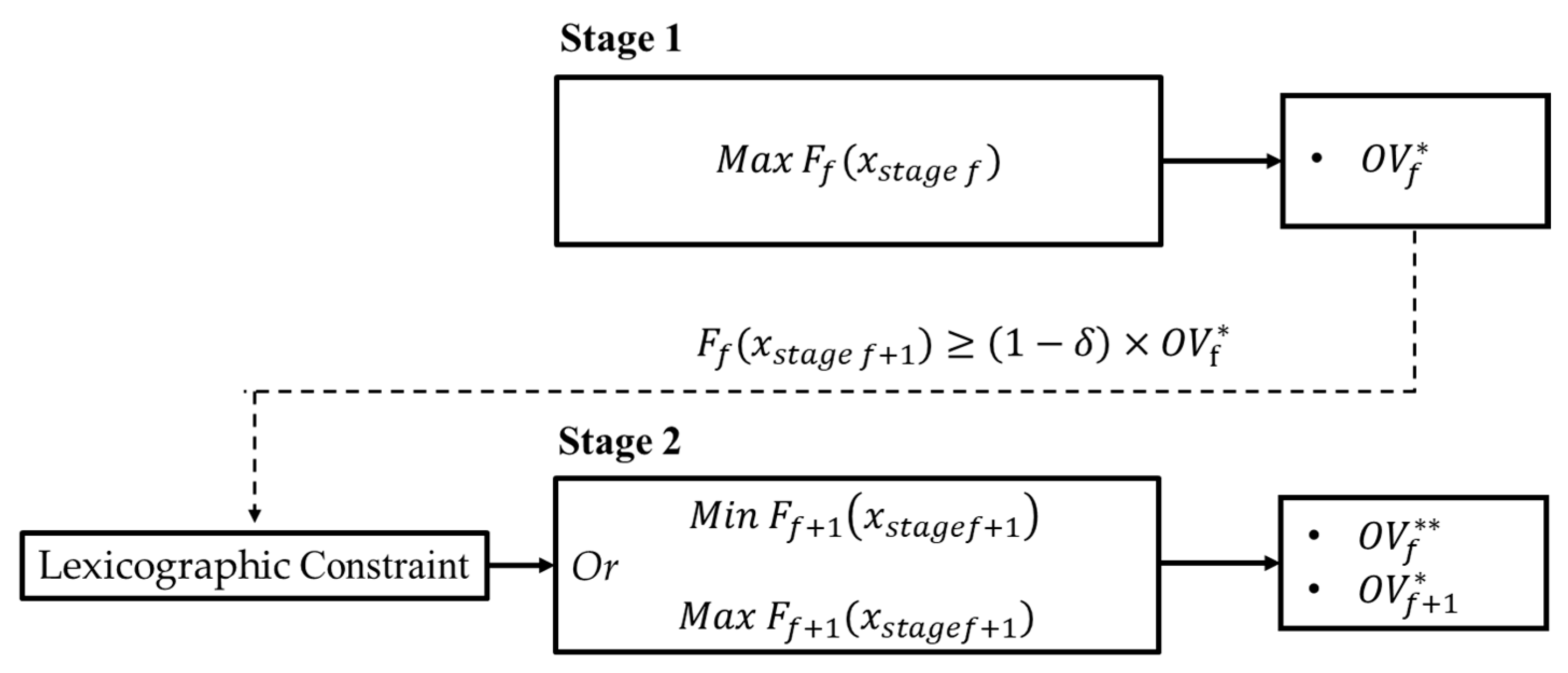
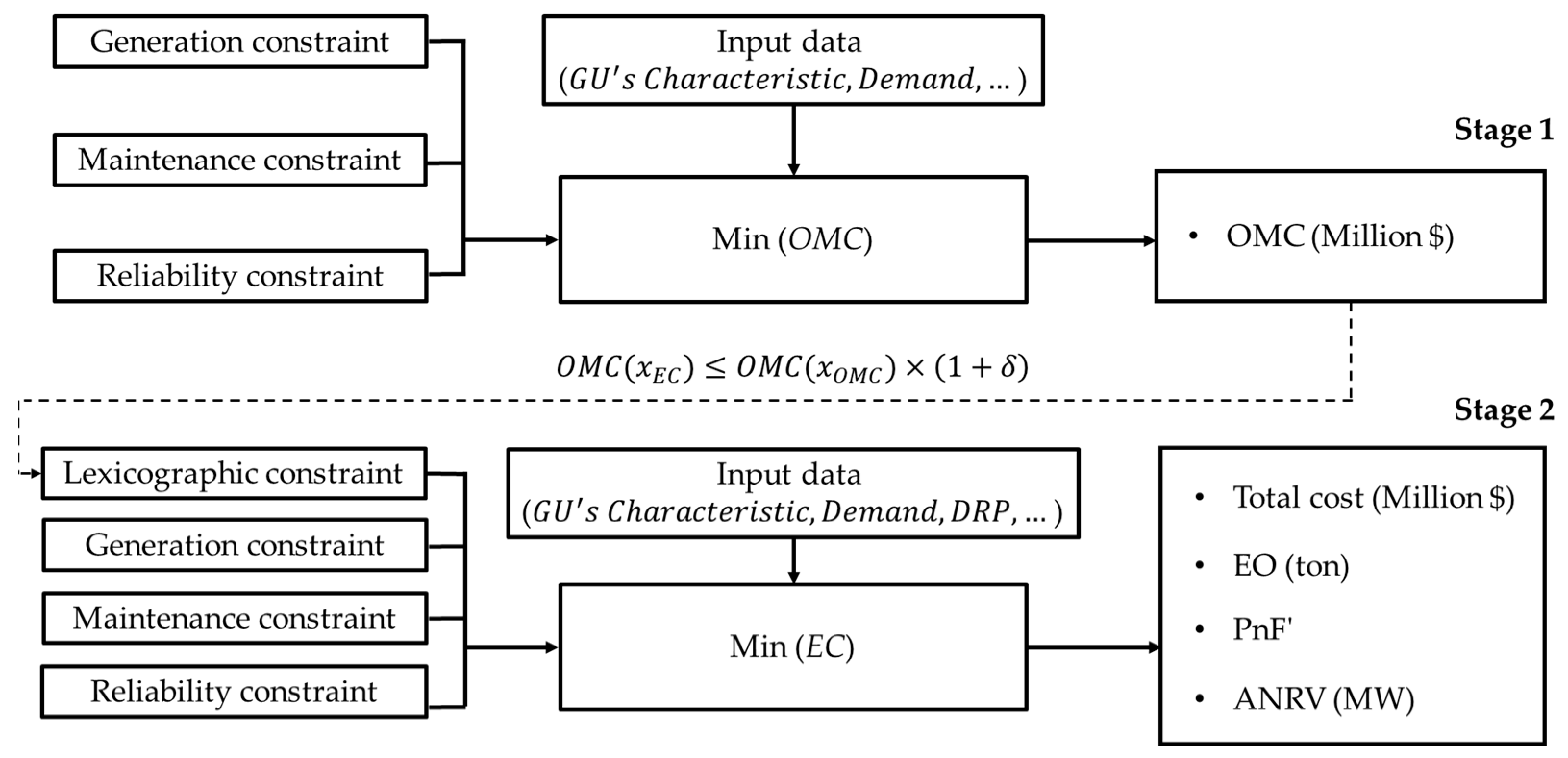
• While recent works have formulated the GMS model by considering the emission output, operation and maintenance costs, and the ANRV, this paper, based on carbon taxation policies forced on GenCos, proposes GMS models focusing on operation, maintenance, and emission costs. These models aim to minimize the sum of operation, maintenance, and emission costs simultaneously and to minimize operation, maintenance, and emission costs at each stage by adapting the lexicographic method. This work aims to support GenCos by lowering their total costs, reducing emissions, and increasing the reliability of the system.
• From the DRP that was used in the GMS problems without consideration of emission costs, the authors adapt the DRP to the GMS model mentioned above (i).
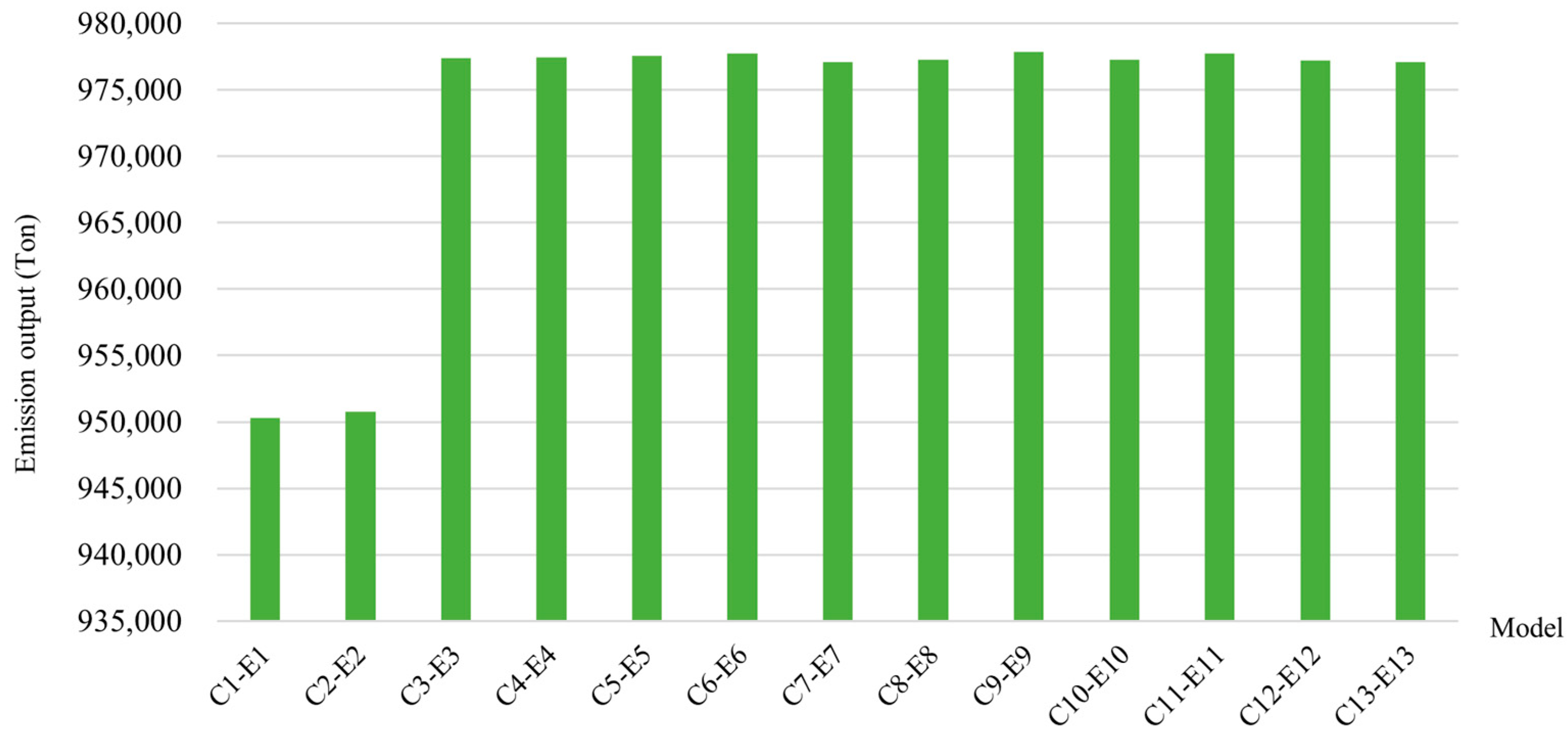
• While the PnF and ANRV are separately shown in previous works, this paper demonstrates both the PnF and ANRV simultaneously to support the decision making of GenCos in terms of system reliability, with and without considering the GU’s FR. The emission output is also depicted to demonstrate the correlation between the total costs, system reliability, and environmental concerns. The emissions cost coefficients are varied to increase the robustness of the results.

The remainder of this paper is organized as follows: The GMS indices, which are the costs, emission output, PnF, and ANVR, are mathematically expressed in Section 2. The lexicographic method is depicted in Section 3, with an illustration of the proposed GMS models in Section 4. Finally, the numerical results are analyzed and summarized in Section 5 and our concluding remarks are in Section 6.

2. GMS Indices and Constraints

This section describes the operation, maintenance, emission, and DRP costs. Also, the PnF, ANRV, and related constraints are demonstrated.

2.1. GMS Indices

The operation and maintenance costs (OMC) expressed in Equation (1) are the main costs included in the GMS problem. They can be divided into two groups. The first depends on the GU’s variable power output ($P_{i,t}$) and variable cost coefficient ($V{C}_i$), whereas the second is correlated with the maintenance cost coefficient ($M{C}_i$). The emission cost (EC) depicted in Equation (2) is based on the emission cost factor (ECC) and emission output ($E{O}_{i,t}$) [35].

$$OMC={\displaystyle \sum }_{t=1}^T{\displaystyle \sum }_{i=1}^I\left[P_{i,t}V{C}_{i}H\left(1-m{s}_{i,t}\right)+M{C}_i\left(m{s}_{i,t}\right)\right]$$

(1)

$$EC=ECC{\displaystyle \sum }_{t=1}^T{\displaystyle \sum }_{i=1}^{I}E{O}_{i,t}$$

(2)

In Equation (3), the $E{O}_{i,t}$ can be calculated by the emission output coefficient ($EO{C}_i$) [35].

$$E{O}_{i,t}=P_{i,t}EO{C}_i\left(1-m{s}_{i,t}\right)H$$

(3)

The average net reserve value (ANRV) shown in Equation (4) is the weekly average capacity reserve depending on the reserve margin value ($RM{V}_t$), the maximum capacity of the GU ($P_i^{Max}$), and the load demand ($D_{b,t}$). The $RM{V}_t$ expressed in Equation (5) is the ratio between the demand and reserve capacity [23].

$$ANRV=\frac{1}{T}{\displaystyle \sum }_{t=1}^{T}RM{V}_t\left[{\displaystyle \sum }_{i=1}^I{P}_i^{Max}\left(1-m{s}_{i,t}\right)-{\displaystyle \sum }_{b=1}^B{D}_{b,t}\right]$$

(4)

$$RM{V}_t={\displaystyle \sum }_{b=1}^B{D}_{b,t}/\left({\displaystyle \sum }_{i=1}^I{P}_i^{Max}-{\displaystyle \sum }_{b=1}^B{D}_{b,t}\right)$$

(5)

The demand response program (DRP) [23,36] has two main categories: (i) the time-based rate program (TBR) with no incentives or penalties for electricity customers; and (ii) the incentive-based rate program (IBR) divided into voluntary, mandatory, and market-based algorithms. This study focuses on the voluntary IBR, providing incentives to customers for reducing their MWh without penalties. The power system is assumed to operate in a smart environment capable of responding to the direct load control and emergency DRP.

The cost of the DRP (DRPC) in Equations (6) and (7) is determined by factors such as the demand ratio ($d{r}_t$), incentive for reducing energy consumption by 1 MWh ($in{c}_b$), and the demand before and after implementing the DRP. The demand ratio in Equation (8) relies on the demand at interval t and the maximum demand across all intervals. In Equation (9), the $D_{b,t}^{DRP}$ is influenced by the market price of electricity, the nominal potential of the responsive load, and the price elasticity of demand [23,32,36].

$$DRPC={\displaystyle \sum }_{t=1}^T{\displaystyle \sum }_{b=1}^{B}DRP{C}_{b,t}$$

(6)

$$DRP{C}_{b,t}=d{r}_{t}in{c}_b\left(D_{b,t}-D_{b,t}^{DRP}\right)$$

(7)

$$d{r}_t=\frac{D_{b,t}}{D_b^{max}}$$

(8)

$$D_{b,t}^{DRP}=\left(1-nd\right)D_{b,t}+nd{D}_{b,t}\left(1+{\displaystyle \sum }_{j=1}^{T}E\left(t,j\right)\times \frac{m{p}_{b,j}^{DR}-m{p}_{b,j}+d{r}_{j}in{c}_b}{m{p}_{b,j}}\right)$$

(9)

where E(t,j) represents the price elasticity between the the price elasticity between the t-th and j-th periods [23,32,36].

The probability that no generation unit fails unexpectedly (PnF), which is described in detail in [22], is based on Equations (10)–(14). In Equation (10), the PnF is influenced by four factors: (i) the GU’s capacity ($P_i^{Max}$), (ii) the GU’s failure rate ($F{R}_i$), (iii) the duration between the GU’s previous and present maintenance ($m_{ps,i}-m_{pv,i}$), and (iv) the generation capacity of the largest GU in the system ($P_{Largest}$). The PnF is converted to Z in Equation (11), indicating that Z should have a low value to reflect the original PnF. To efficiently obtain the results, as shown in Equations (12)–(14), the natural logarithm is used to linearize the model. The linearized Z is represented by PnF’, which should also have a low value, similar to that for Z [22,34].

$$PnF={\displaystyle \prod }_i{\left[\frac{1}{exp\left(-F{R}_i\left(m_{ps,i}-m_{pv,i}-1\right)\right)}\right]}^{\frac{P_i^{Max}}{P_{Largest}}}$$

(10)

$$Z={\displaystyle \prod }_i{\left[exp\left(-F{R}_i\left(m_{ps,i}-m_{pv,i}-1\right)\right)\right]}^{-\frac{P_i^{Max}}{P_{Largest}}}$$

(11)

$$Pn{F}^{\prime }=\ln \left(Z\right)$$

(12)

$$Pn{F}^{\prime }={\displaystyle \sum }_{i=1}^I-\frac{P_i^{Max}}{P_{Largest}}ln\left[exp\left(-F{R}_i\left(m_{ps,i}-m_{pv,i}-1\right)\right)\right]$$

(13)

$$Pn{F}^{\prime }={\displaystyle \sum }_{i=1}^I\frac{P_i^{Max}}{P_{Largest}}\left[F{R}_i\left(m_{ps,i}-m_{pv,i}-1\right)\right]$$

(14)

2.2. Constraints of GMS

To efficiently maintain the GU and secure the power system, the operation, maintenance, and power generation constraints must be satisfied [22,23,25,34].

$${\displaystyle \sum }_{t=1}^{T}m{s}_{i,t}=d_i$$

(15)

$$m{s}_{i,t}-m{s}_{i,t-1}\le m{s}_{i,t+d_i-1}$$

(16)

$${\displaystyle \sum }_{t=1}^{T}im{s}_{i,t}=1$$

(17)

$$m{s}_{i,t}+p{s}_{i,t}\le 1$$

(18)

$$(1-m{s}_{i,t})P_i^{Min}\le P_{i,t}\le (1-m{s}_{i,t})P_i^{Max}$$

(19)

$${\displaystyle \sum }_{i=1}^I{P}_{i,t}\ge {\displaystyle \sum }_{b=1}^B{D}_{b,t}$$

(20)

The maintenance duration is denoted by Equation (15), whereas the outage continuity is determined by Equation (16), while Equations (17) and (18) guarantee that the GU will be maintained once a horizon and satisfy the relationship between the GU’s maintenance and production states, respectively. The GU’s output limitation is defined in Equation (19). The total power output, without considering the power loss, must be higher than or equal to the load demand to preserve the system’s security, as demonstrated in Equation (20).

3. The Multi-Objective Optimization Method

The lexicographic method is used to track the multi-objective optimization problem with all objectives hierarchically solved in their own stage depending on the adjustable coefficient. The advantage is that each objective can be focused on and analyzed independently. Nonetheless, a suitable coefficient is difficult to find.

For the mathematical model, if the first objective is to minimize the value, the function is shown in Equation (21). In the second stage, as depicted in Equation (22), the models can be maximization or minimization problems, with the constraint defined in Equation (23) [23,37].

$$O{V}_f^{*}=\min F_f\left(x_{stage f}\right)$$

(21)

$$O{V}_{f+1}^{*}=\mathrm{Min} \mathrm{or} \mathrm{Max}{F}_{f+1}\left(x_{stagef+1}\right)$$

(22)

Subject to

$$F_f\left(x_{stage f+1}\right)\le \left(1+\delta \right)\times O{V}_{\mathrm{f}}^{*}$$

(23)

where $x_{stage f}$ and $x_{stage f+1}$ are sets of variables used to obtain the results in the first and second stages, respectively. From Equation (23), the $\delta$ is used to relax the search space for the second optimization problem with a value between 0 and 1.

$$O{V}_f^{*}=\max F_f\left(x_{stage f}\right)$$

(24)

Subject to

$$F_f\left(x_{stage f+1}\right)\ge \left(1-\delta \right)\times O{V}_f^{*}$$

(25)

On the other hand, if the maximization model is run first, as shown in Equation (24), the function and constraint of the second stage can be expressed as Equations (22) and (25), respectively.

The lexicographic method can also be illustrated as shown in Figure 1 and Figure 2.

4. The Hierarchy of the Proposed GMS Models

To obtain the costs of the GMS, emission output, PnF’, and ANRV, the GMS models are proposed and illustrated in this section.

Model A: The objective function is to minimize the OMC and EC simultaneously. The OMC and EC can be tracked by using the equations defined in Section 2.

$$\mathrm{Min} \left(OMC+EC\right)$$

(26)

Subject to

Constraints (15)–(20)

Model B: The OMC is first minimized, and the EC is solved in the second stage using the definition of the lexicographic method depicted in Section 3. In Equation (29), the OMC based on the GMS plan in the second stage must be less than or equal to the previous OMC multiplied by the lexicographic coefficient.

Stage 1:

$$\mathrm{Min} \left(OMC\right)$$

(27)

Subject to

Constraints (15)–(20)

Stage 2:

$$\mathrm{Min} \left(EC\right)$$

(28)

Subject to

Constraints (15)–(20)

$$OMC\left(x_{EC}\right)\le OMC\left(x_{OMC}\right)\times \left(1+\delta \right)$$

(29)

Model C: This model runs the GMS problems considering the EC and OMC minimization consecutively.

Stage 1:

$$\mathrm{Min} \left(EC\right)$$

(30)

Subject to

Constraints (15)–(20)

Stage 2:

$$\mathrm{Min} \left(OMC\right)$$

(31)

Subject to

Constraints (15)–(20)

$$EC\left(x_{OMC}\right)\le EC\left(x_{EC}\right)\times \left(1+\delta \right)$$

(32)

Model D: To validate the advantage of the proposed GMS models, the GMS problem presented in [23] is also adapted and solved. The mathematical equations are as follows:

Stage 1:

$$\mathrm{Min} \left(EO\right)$$

(33)

Subject to

Constraints (15)–(20)

Stage 2:

$$\mathrm{Min} \left(OMC\right)$$

(34)

Subject to

Constraints (15)–(20)

$$EO\left(x_{OMC}\right)\le EO\left(x_{EO}\right)\times \left(1+\delta \right)$$

(35)

Stage 3:

$$\mathrm{Max} \left(ANRV\right)$$

(36)

Subject to

Constraints (15)–(20)

$$EO\left(x_{ANRV}\right)\le EO\left(x_{OMC}\right)\times \left(1+\delta \right)$$

(37)

$$OMC\left(x_{ANRV}\right)\le OMC\left(x_{OMC}\right)\times \left(1+\delta \right)$$

(38)

where Equations (37) and (38) are the constraints obtained from stage 2.

Model E: In this model, the DRP is adapted to the GMS problem to identify the benefits of the financial costs, emission generation, and system reliability. The mathematical model is proposed as follows:

Stage 1:

$$\mathrm{Min} \left(EC\right)$$

(39)

Subject to

Constraints (15)–(20)

Stage 2:

$$\mathrm{Min} \left(OMC+DRPC\right)$$

(40)

Subject to

Constraints (15)–(19)

$${\displaystyle \sum }_{i=1}^I{P}_{i,t}\ge {\displaystyle \sum }_{b=1}^B{D}_{b,t}^{DRP}$$

(41)

$$EC\left(x_{OMC,DRP}\right)\le EC\left(x_{EC}\right)\times \left(1+\delta \right)$$

(42)

where $x_{OMC,DRP}$ is the GMS plan obtained by adapting the DRP to the GMS model.

Figure 3, Figure 4, Figure 5, Figure 6 and Figure 7 illustrate all the GMS models. Only model A is run in a single stage calculation, whereas models B and C are solved as two-stage problems. In model D, the results are obtained by minimizing the emission output, minimizing the total cost, and maximizing the ANRV consecutively. Model E is the same as depicted in model C, but the DRP is adapted in the second stage. With these GMS algorithms, the numerical results are shown in Section 5.

5. Numerical Results

The IEEE 24-bus reliability test system [38] is used to numerically demonstrate the results of the proposed GMS models. For the characteristics of GUs, their generation capacity and maintenance duration can be obtained from [22,35,39]. The $M{C}_i$, $V{C}_i$, and $EO{C}_i$ are denoted by [35]. The GU’s $F{R}_i$ and $m_{pv,i}$ are shown in [22,39]. The $m{p}_{b,j}$ and $D_{b,t}$ are extracted from [25] and [20,38], respectively. To find the results, there is an assumption that the load demand and electricity price are certain [20,22,23,25,34], while the power loss is not considered. The T is divided into 52 weeks, based on yearly maintenance scheduling, whereas the H is 24 × 7 = 168 h. The $\mathsf{\delta }$ is assumed to be 0.1 (10%) [23]. The nominal potential of DRPs is 10% of the total load, and the weekly price elasticity of the load can be extracted from [36].

To increase the robustness and demonstrate the tendency of the results, all the GMS models are run for thirteen cases, in which the emission cost coefficients vary from 28 to 40 USD/ton. The values of 28, 35, and 40 USD/ton are from [3,4,5], respectively. The values of 29, 30, 31, 32, 33, 34, 36, 37, 38, and 39 USD/ton are specifically chosen by the authors. It is expected that the models can still benefit GenCos when the emission cost coefficient is not constant. The GMS problems are investigated using the optimization function in the MATLAB program, running on a computer with an AMD Ryzen 7 3750H Gfx 2.30 GHz processor and 16.0 GB of RAM.

5.1. Preliminary Verification of the Results

Based on the previous results [22,23,24,25,40] and issues mentioned in Section 1, the GUs should be maintained in low-demand intervals. This is because the GenCo has a high difference between its maximum and used generation capacities., This has led to high system reliability and low maintenance costs. On the other hand, the GenCo may have to purchase electricity from other sources to supply its load and its reserve generation capacity may not be satisfied if the GUs are shut down in high-demand intervals. Considering the results of this paper, the unused generation capacities based on models A, D, and E are shown in Figure 8, Figure 9 and Figure 10, respectively. These models are selected because they have different procedures to obtain the results, as explained in Section 4. Also, cases 1, 8, and 13 are based on 28, 35, and 40 USD/ton emission cost coefficients, as reported by [3,4,5], respectively. The results show that most GUs are maintained in low-demand intervals, which are weeks 9–15 and 31–42, as specified by the load data [20,38]. It can be said that the results found in this paper are reliable, robust, and consistent with those of previous studies. We have neglected to show the unused capacities of models B and C to avoid providing a redundant analysis.

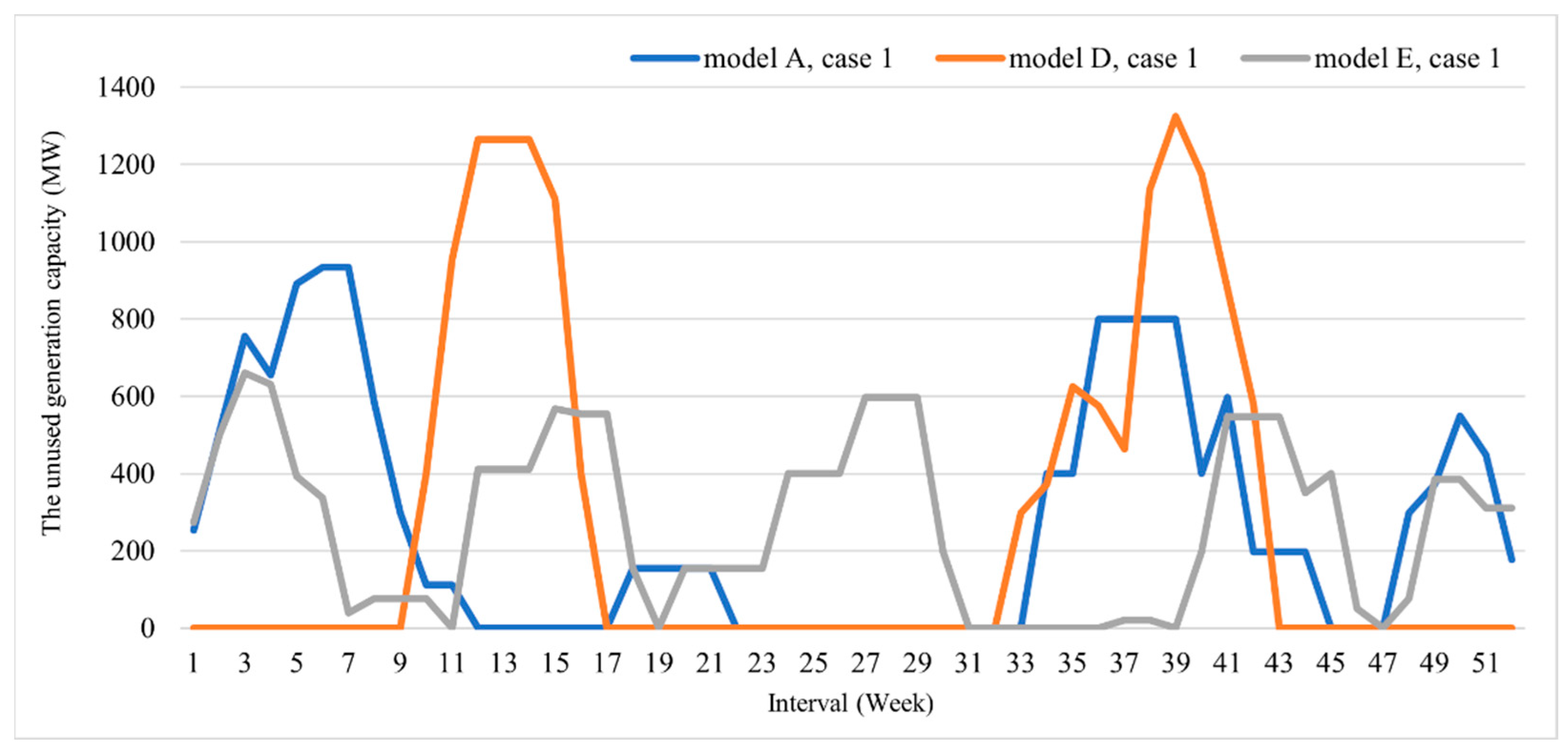
5.2. The Results of Models A, B, and C

The GMS indices from models A, B, and C are demonstrated in

Table 2. The total cost, emission output, PnF’, and ANRV from models A, B, and C.

Case	Model	Total Cost (Million USD)	Emission Output (Million ton)	PnF’	ANRV (MW)
1	A	1309.622	9.622	67.30	1704
	B	1317.550	9.426	56.82	1733
	C	1309.697	9.615	57.34	1740
2	A	1319.884	9.615	68.51	1673
	B	1326.977	9.426	59.23	1733
	C	1319.308	9.616	57.34	1740
3	A	1329.855	9.624	67.50	1655
	B	1336.403	9.426	59.24	1808
	C	1328.921	9.616	57.34	1740
4	A	1340.802	9.620	60.64	1657
	B	1345.830	9.426	64.71	1770
	C	1338.537	9.616	57.34	1740
5	A	1347.141	9.618	62.64	1757
	B	1355.256	9.426	55.29	1742
	C	1348.155	9.616	57.34	1740
6	A	1357.269	9.622	63.01	1699
	B	1364.682	9.426	60.75	1683
	C	1357.774	9.616	57.34	1740
7	A	1367.794	9.619	63.25	1699
	B	1374.317	9.433	63.23	1614
	C	1367.391	9.615	57.34	1740
8	A	1376.883	9.632	69.31	1717
	B	1383.535	9.426	65.93	1751
	C	1377.002	9.616	57.34	1740
9	A	1384.011	9.636	60.69	1768
	B	1392.962	9.426	59.59	1718
	C	1386.626	9.616	57.34	1740
10	A	1397.675	9.616	58.15	1675
	B	1402.388	9.426	56.26	1716
	C	1396.234	9.616	57.34	1740
11	A	1403.410	9.580	69.72	1673
	B	1411.815	9.426	60.27	1712
	C	1405.855	9.616	57.34	1740
12	A	1415.777	9.635	63.01	1614
	B	1421.241	9.426	60.88	1663
	C	1415.466	9.615	57.34	1740
13	A	1427.110	9.602	68.74	1615
	B	1430.667	9.426	61.62	1740
	C	1425.084	9.615	57.34	1740

, showing that model A gives the minimum costs in cases 1, 5, 6, 8, 9, and 11, while model C is the best choice for cases 2, 3, 4, 7, 10, 12, and 13. To find the optimal GMS plan, if the GenCo only considers the total cost, models A and C should be run. On the other hand, model B is not appropriate for all cases.

If both the total cost and emission output are considered by the GenCo, the differences among the costs of models A, B, and C are depicted in Figure 11. On the x-axis, B1–A1 and B1–C1 represent the gaps in costs between models B and A and models B and C, respectively, for case 1. The Figure indicates that model B consistently results in higher costs in all cases. However, the differences among the emission outputs of the three models are shown in Figure 12, in which the terms on the x-axis can be logically explained as those in Figure 11. It can be observed that model B consistently generates lower emissions in all cases as well. Therefore, if emission concerns are correlated to crucial issues such as government policies, carbon credits, and sustainable development goals, choosing model B can lead to significant benefits for GenCos.

When considering all indices, which are the total costs, emission output, PnF’, and ANRV, GenCos should select model C in cases 2, 7, and 12, whereas model A is appropriate for cases 5 and 9. Model B is not considered in all cases because it has very high costs compared to those of models A and C. By contrast, if a GenCo benefits from system reliability, such as reliability charges, and market power to negotiate with its customers, model C is the attractive choice for cases 1, 3, 4, 6, 8, 10, 11, and 13.

The results indicate the following: (i) A GMS model that only includes the OMC and EC in a single state do not benefit GenCos in some cases; (ii) GenCos have the flexibility to choose a GMS plan based on their considerations, including their financial management, emission concerns, and system reliability; and (iii) If the emission output is not a primary concern or if reducing the running time is a priority, it is reasonable to discard model B, as it consistently leads to higher costs compared to those of models A and C.

5.3. The Results of Models C and D

To demonstrate the robustness of the proposed GMS models, the GMS problem discussed in [23], represented by model D, is adapted and solved. The outcomes of model C are chosen as the benchmark in this section for the following reasons: (i) This model adopts the lexicographic method, as implemented in model D; (ii) Displaying the total costs of model A would present redundant data, which can be avoided; and (iii) Model B is not suitable for cost minimization in any of the cases, as illustrated in Section 5.2.

In

Table 3. The total cost, emission output, PnF’, and ANRV from models C and D.

Case	Model	Total Cost (Million $)	Emission Output (Million ton)	PnF’	ANRV (MW)
1	C	1309.697	9.615	57.34	1740
	D	1310.591	9.812	74.35	1907
2	C	1319.308	9.616	57.34	1740
	D	1320.404	9.812	74.35	1907
3	C	1328.921	9.616	57.34	1740
	D	1330.216	9.812	74.35	1907
4	C	1338.537	9.616	57.34	1740
	D	1340.028	9.812	74.35	1907
5	C	1348.155	9.616	57.34	1740
	D	1349.840	9.812	74.35	1907
6	C	1357.774	9.616	57.34	1740
	D	1359.652	9.812	74.35	1907
7	C	1367.391	9.615	57.34	1740
	D	1369.464	9.812	74.35	1907
8	C	1377.002	9.616	57.34	1740
	D	1379.276	9.812	74.35	1907
9	C	1386.626	9.616	57.34	1740
	D	1389.088	9.812	74.35	1907
10	C	1396.234	9.616	57.34	1740
	D	1398.900	9.812	74.35	1907
11	C	1405.855	9.616	57.34	1740
	D	1408.712	9.812	74.35	1907
12	C	1415.466	9.615	57.34	1740
	D	1418.524	9.812	74.35	1907
13	C	1425.084	9.615	57.34	1740
	D	1428.336	9.812	74.35	1907

, the results indicate that model D achieves the highest ANRV in all cases. This high performance can be attributed to the model’s emphasis on system reliability. Figure 13 and Figure 14 demonstrate the gaps in costs and emission outputs between models C and D, respectively. When comparing the total costs of models C and D, as depicted in Table 3 and Figure 13, model D incurs significantly higher costs than model C in all cases. Additionally, considering the emission outputs shown in Table 3 and Figure 14, model D also generates the highest emissions in all cases. This implies that the proposed GMS models in this paper outperform the model presented in the previously published work when the cost of emissions is taken into account in the GMS problems.

5.4. The Results of Models C and E

To decrease the total financial cost, reduce the generation of emissions, and increase the system reliability, the implementation of the DRP is numerically solved.

The results for the cost, emission output, PnF’, and ANRV of models C and E are presented in

Table 4. The total cost, emission output, PnF’, and ANRV from models C and E.

Case	Model	Total Cost (Million USD)	Emission Output (Million tons)	PnF’	ANRV (MW)
1	C	1309.697	9.615	57.34	1740
	E	1247.733	8.665	68.88	1681
2	C	1319.308	9.616	57.34	1740
	E	1256.398	8.665	68.88	1681
3	C	1328.921	9.616	57.34	1740
	E	1265.045	8.638	64.94	1727
4	C	1338.537	9.616	57.34	1740
	E	1273.683	8.638	64.94	1727
5	C	1348.155	9.616	57.34	1740
	E	1282.321	8.638	64.94	1727
6	C	1357.774	9.616	57.34	1740
	E	1290.960	8.638	64.94	1727
7	C	1367.391	9.615	57.34	1740
	E	1299.598	8.638	64.94	1727
8	C	1377.002	9.616	57.34	1740
	E	1308.236	8.638	64.94	1727
9	C	1386.626	9.616	57.34	1740
	E	1316.875	8.638	64.94	1727
10	C	1396.234	9.616	57.34	1740
	E	1325.513	8.638	68.88	1681
11	C	1405.855	9.616	57.34	1740
	E	1334.151	8.638	68.88	1681
12	C	1415.466	9.615	57.34	1740
	E	1342.789	8.638	64.94	1727
13	C	1425.084	9.615	57.34	1740
	E	1351.428	8.638	64.94	1727

. The costs of model E are 4.73%, 4.77%, 4.81%, 4.85%, 4.88%, 4.92%, 4.96%, 4.99%, 5.03%, 5.07%, 5.10%, 5.13%, and 5.17% lower than those of model C for cases 1–13, respectively. The corresponding cost values (in USD) are illustrated in Figure 15. Furthermore, the differences between the emission outputs of models C and E are 9.88%, 9.89%, 10.16%, 10.17%, 10.17%, 10.17%, 10.16%, 10.16%, 10.17%, 10.16%, 10.17%, 10.16%, and 10.16% for cases 1–13, respectively, with the values as tons depicted in Figure 16. In terms of system reliability, the PnF’ indices generated by model E are slightly higher than those of model C, although the differences are negligible compared to the benefits received from the cost and emission reductions. Furthermore, the ANRVs in all cases meet the desired values compared to those of model C. Consequently, incorporating the DRP into the GMS plan proves to be a superior choice. However, GenCos need to find efficient solutions for operating the DRP in real scenarios, considering recent works proposing DRP applications [41,42,43,44] that can be later adapted to the GMS field.

6. Conclusions

In this paper, four GMS models, represented by A, B, C, and E, are proposed to identify the minimum total cost paid by GenCos. Model A minimizes the sum of the OMC and EC in a single stage. Model B aims to find the minimum OMC and EC consecutively. Model C is used to solve the minimum EC and OMC consecutively. In model E, the EC, OMC, and DRP are minimized in three stages. The last three models are calculated by using the lexicographic method as a mathematical tool. To demonstrate the robustness of the proposed GMS algorithms, the GMS model in a previously published work, which hieratically aims to minimize the emission output, minimize the OMC, and maximize the ANRV, is also run. It is represented by model D. All models are tracked based on thirteen cases following the emission cost coefficients of 28–40 USD/ton. The IEEE 24-bus reliability test system is implemented to obtain numerical results. GMS indices such as the emission output, PnF, and ANRV are demonstrated to support the GenCo’s decision.

The results show the following: (i) When the emission cost is considered as one of the objective functions, models A and C result in the minimum costs in several cases and should be primarily chosen by the GenCo. Significantly, they provide a balance between cost minimization and emission reduction; (ii) Model B has the highest costs in all cases. However, it generates the lowest emissions. If the emission factor has benefits beyond financial aspects, such as corporate social responsibility, social welfare, sustainable development goals, or the potential to adapt carbon credits to the GenCo, this model can be a suitable algorithm; (iii) Model D is a better choice when the GenCo prioritizes system reliability, especially in terms of its generation capacity. The GenCo can ensure the reliability of its power supply to its customers, which can be advantageous in terms of customer satisfaction. However, this model generates significantly high costs and emission outputs compared to those of models A, C, and E; (iv) Model E consistently has the lowest costs and emission outputs in all cases. Nonetheless, it requires the implementation of the DRP in collaboration with customers. This model can be considered when a GenCo has the capability to work with customers to optimize their demand response strategies. From the perspective of the ISO, there are no concerns because all models satisfy all of the crucial constraints. Therefore, the selection of a specific model depends on the priorities and objectives of the GenCo, such as cost minimization, emission reductions, system reliability maximization, and collaboration with customers through the DRP.

Therefore, in certain cases, GenCos cannot achieve the minimum cost by including the OMC and EC in a single objective function. Better results can be obtained by adapting the lexicographic method to the GMS problem. Additionally, our GMS models yield superior outcomes compared to those of previous works, offering benefits for GenCos in various aspects such as financial management, carbon taxation, and system reliability.

However, the models presented in this paper were not solved with actual parameters based on specific electricity generation and carbon tax policies in any country. Hence, for future work, it would be beneficial to incorporate carbon credit, government policies, and social welfare into the objective function, while using actual data in the models. Furthermore, the proposed GMS models can be applied in competitive markets using game theory to optimally satisfy the objectives of GenCos.

References

1. Endrenyi, J.; Aboresheid, S.; Allan, R.N.; Anders, G.J.; Asgarpoor, S.; Billinton, R.; Chowdhury, N.; Dialynas, E.N.; Fipper, M.; Fletcher, R.H.; et al. The present status of maintenance strategies and the impact of maintenance on reliability. IEEE Trans. Power Syst. 2001, 16, 638–646. [Google Scholar] [CrossRef]
2. Endrenyi, J.; Anders, G.J.; Leite da Silva, A.M. Probabilistic evaluation of the effect of maintenance on reliability—An application. IEEE Trans. Power Syst. 1998, 13, 576–583. [Google Scholar] [CrossRef] [PubMed]
3. Resources for the Future. Carbon Pricing 201: Pricing Carbon in the Electricity Sector. Available online: https://www.rff.org/publications/explainers/carbon-pricing-201-pricing-carbon-electricity-sector/ (accessed on 15 August 2022).
4. International Energy Agency. The Potential Role of Carbon Pricing in Thailand’s Power Sector. Thailand, 2021. Available online: https://www.iea.org/reports/the-potential-role-of-carbon-pricing-in-thailands-power-sector (accessed on 15 August 2022).
5. Parry, I. Putting a Price on Pollution. Available online: https://www.imf.org/Publications/fandd/issues/2019/12/the-case-for-carbon-taxation-and-putting-a-price-on-pollution-parry (accessed on 15 August 2022).
6. Leroutier, M. Carbon pricing and power sector decarbonization: Evidence from the UK. J. Environ. Econ. Manag 2022, 111, 102580. [Google Scholar] [CrossRef]
7. Lovcha, Y.; Perez-Laborda, A.; Sikora, I. The determinants of CO2 prices in the EU emission trading system. Appl. Energy 2022, 305, 117903. [Google Scholar] [CrossRef]
8. Handayani, K.; Anugrah, P.; Goembira, F.; Overland, I.; Suryadi, B.; Swandaru, A. Moving beyond the NDCs: ASEAN pathways to a net-zero emissions power sector in 2050. Appl. Energy 2022, 311, 118580. [Google Scholar] [CrossRef]
9. Olmstead, E.H.; Yatchew, A. Carbon pricing and Alberta’s energy-only electricity market. Electr. J. 2022, 35, 107112. [Google Scholar] [CrossRef]
10. Wong, J.B.; Zhang, Q. Impact of carbon tax on electricity prices and behaviour. Finance. Res. Lett. 2022, 44, 102098. [Google Scholar] [CrossRef]
11. Köppl, A.; Schratzenstaller, M. Carbon taxation: A review of the empirical literature. J. Econ. Surv. 2023, 37, 1353–1388. [Google Scholar] [CrossRef]
12. Hasnu, F.N.M.; Muhammad, I. Environmental issues in Malaysia: Suggestion to impose carbon tax. Asia Pac. Manag. Account. J. 2022, 17, 65–95. [Google Scholar]
13. Muhammad, I. Carbon tax as the most appropriate carbon pricing mechanism for developing countries and strategies to design an effective policy. AIMS Environ. Sci. 2022, 9, 145–168. [Google Scholar] [CrossRef]
14. Chien, F.S.; Vu, T.L.; Phan, T.T.H.; Van Nguyen, S.; Anh, N.H.V.; Ngo, T.Q. Zero-carbon energy transition in ASEAN countries: The role of carbon finance, carbon taxes, and sustainable energy technologies. Renew. Energy 2023, 212, 561–569. [Google Scholar] [CrossRef]
15. Sadeghian, O.; Shotorbani, A.M.; Mohammadi-Ivatloo, B. Generation maintenance scheduling in virtual power plants. IET Gener. Transm. Distrib. 2019, 13, 2584–2596. [Google Scholar] [CrossRef]
16. Bagheri, B.; Amjady, N.; Dehghan, S. Multiscale multiresolution generation maintenance scheduling: A stochastic affinely adjustable robust approach. IEEE Sys. J. 2021, 15, 893–904. [Google Scholar] [CrossRef]
17. Lou, X.; Feng, C.; Chen, W.; Guo, C. Risk-based coordination of maintenance scheduling and unit commitment in power systems. IEEE Access 2020, 8, 58788–58799. [Google Scholar] [CrossRef]
18. Zhang, Z.; Liu, M.; Xie, M.; Dong, P. A mathematical programming–based heuristic for coordinated hydrothermal generator maintenance scheduling and long-term unit commitment. J. Electr. Power. Energy Syst. 2023, 147, 108833. [Google Scholar] [CrossRef]
19. Sadeghian, O.; Shotorbani, A.M.; Mohammadi-Ivatloo, B. Risk-based stochastic short-term maintenance scheduling of GenCos in an oligopolistic electricity market considering the long-term plan. Electr. Power Syst. Res. 2019, 175, 105908. [Google Scholar] [CrossRef]
20. Hassanpour, A.; Roghanian, E. A two-stage stochastic programming approach for non-cooperative. J. Electr. Power Energy Syst. 2021, 126, 106584. [Google Scholar] [CrossRef]
21. Rokhforoz, P.; Gjorgiev, B.; Sansavini, G.; Fink, O. Multi-agent maintenance scheduling based on the coordination between central operator and decentralized producers in an electricity market. Reliab. Eng. Syst. Saf. 2021, 210, 107495. [Google Scholar] [CrossRef]
22. Eygelaar, J.; Lötter, D.P.; Vuuren, J.H. Generator maintenance scheduling based on the risk of power generating unit failure. J. Electr. Power Energy Syst. 2018, 95, 83–95. [Google Scholar] [CrossRef]
23. Mollahassani-Pour, M.; Rashidinejad, M.; Pourakbari-Kasmaei, M. Environmentally constrained reliability-based generation maintenance scheduling considering demand-side management. IET Gener. Transm. Distrib. 2019, 13, 1153–1163. [Google Scholar] [CrossRef]
24. Lindner, B.G.; Brits, R.; Vuuren, J.H.; Bekker, J. Tradeoffs between levelling the reserve margin and minimising production cost in generator maintenance scheduling for regulated power systems. J. Electr. Power Energy Syst. 2018, 101, 458–471. [Google Scholar] [CrossRef]
25. Sadeghian, O.; Oshnoei, A.; Nikkhah, S.; Mohammadi-Ivatloo1, B. Multi-objective optimisation of generation maintenance scheduling in restructured power systems based on global criterion method. IET Gener. Transm. Distrib. 2019, 2, 203–213. [Google Scholar] [CrossRef]
26. Moghbeli, M.; Sharifi, V.; Abdollahi, A.; Rashidinejad, M. Evaluating the impact of energy efficiency programs on generation maintenance scheduling. J. Electr. Power Energy Syst. 2020, 119, 105909. [Google Scholar] [CrossRef]
27. Assis, F.A.; Silva, A.M.; Resende, L.C. Generation maintenance scheduling with renewable sources based on production and reliability costs. Int. J. Electr. Power Energy Syst. 2022, 134, 107370. [Google Scholar] [CrossRef]
28. Martin, L.S.; Yang, J.; Liu, Y. Hybrid NSGA III/dual simplex approach to generation and transmission maintenance scheduling. J. Electr. Power Energy Syst. 2022, 135, 107498. [Google Scholar] [CrossRef]
29. Sharifi, V.; Abdollahi, A.; Rashidinejad, M. Flexibility-based generation maintenance scheduling in presence of uncertain wind power plants forecasted by deep learning considering demand response programs portfolio. J. Electr. Power Energy Syst. 2022, 141, 108225. [Google Scholar] [CrossRef]
30. Salarkheili, S.; Nazar, M.S.; Wozabal, D.; Jabari, F. Capacity withholding of GenCos in electricity markets using security-constrained generation maintenance scheduling. J. Electr. Power Energy Syst. 2023, 146, 108771. [Google Scholar] [CrossRef]
31. Rokhforoz, P.; Montazeri, M.; Fink, O. Safe multi-agent deep reinforcement learning for joint bidding and maintenance scheduling of generation units. Reliab. Eng. Syst. Saf. 2023, 232, 109081. [Google Scholar] [CrossRef]
32. Mollahassani-pour, M.; Rashidinejad, M.; Abdollahi, A. Appraisal of eco-friendly preventive maintenance scheduling strategy impacts on GHG emissions mitigation in smart grids. J. Clean Prod. 2017, 43, 212–223. [Google Scholar] [CrossRef]
33. Sharifi, V.; Abdollahi, A.; Rashidinejad, M.; Heydarian-Forushani, E.; Alhelou, H.H. Integrated electricity and natural gas demand response in flexibility-based generation maintenance scheduling. IEEE Access 2022, 10, 76021–76030. [Google Scholar] [CrossRef]
34. Prukpanit, P.; Kaewprapha, P.; Leeprechanon, N. Optimal generation maintenance scheduling considering financial return and unexpected failure of distributed generation. IET Gener. Transm. Distrib. 2021, 15, 1787–1797. [Google Scholar] [CrossRef]
35. Hemmati, R.; Saboori, H.; Jirdehi, A.M. Multistage generation expansion planning incorporating large scale energy storage systems and environmental pollution. Renew. Energy 2016, 97, 636–645. [Google Scholar] [CrossRef]
36. Abdollahi, A.; Moghaddam, M.P.; Rashidinejad, M.; Sheikh-El-Eslami, M.K. Investigation of economic and environmental-driven demand response measures incorporating UC. IEEE Trans. Smart Grid. 2012, 3, 12–25. [Google Scholar] [CrossRef]
37. Marler, R.T.; Arora, J.S. Survey of multi-objective optimization methods for engineering. Struct. Multidiscip. Optim. 2004, 26, 369–395. [Google Scholar] [CrossRef]
38. Subcommittee, P.M. IEEE reliability test system. IEEE Trans. Power Appar. Syst. 1979, 98, 2047–2054. [Google Scholar] [CrossRef]
39. Schlunz, E.B. Decision Support for Generator Maintenance Scheduling in the Energy Sector; Master of Science, Department of Logistics, Stellenbosch University: Stellenbosch, South Africa, 2011. [Google Scholar]
40. Lakshminarayanan, S.; Kaur, D. Optimal maintenance scheduling of generator units using discrete integer cuckoo search optimization algorithm. Swarm. Evol. Comput. 2018, 42, 89–98. [Google Scholar] [CrossRef]
41. Mansouri, S.A.; Maroufi, S.; Ahmarinejad, A. A tri-layer stochastic framework to manage electricity market within a smart community in the presence of energy storage systems. J. Energy Storage 2023, 71, 108130. [Google Scholar] [CrossRef]
42. Fatemi, S.; Ketabi, A.; Mansouri, S.A. A multi-level multi-objective strategy for eco-environmental management of electricity market among micro-grids under high penetration of smart homes, plug-in electric vehicles and energy storage devices. J. Energy Storage 2023, 67, 107632. [Google Scholar] [CrossRef]
43. Xu, H.; Chang, Y.; Zhao, Y.; Wang, F. A new multi-timescale optimal scheduling model considering wind power uncertainty and demand response. J. Electr. Power Energy Syst. 2023, 147, 108832. [Google Scholar] [CrossRef]
44. Mansouri, S.A.; Jordehi, A.R.; Marzband, M.; Tostado-V´eliz, M.; Jurado, F.; Aguado, J.A. An IoT-enabled hierarchical decentralized framework for multi-energy microgrids market management in the presence of smart prosumers using a deep learning-based forecaster. Appl. Energy 2023, 333, 120560. [Google Scholar] [CrossRef]
Figure 1. Description of minimization problem in the lexicographic method.
Energies 16 07775 g001
Figure 2. Description of maximization problem in the lexicographic method.
Energies 16 07775 g002
Figure 3. The description of model A.
Energies 16 07775 g003
Figure 4. The description of model B.
Energies 16 07775 g004
Figure 5. The description of model C.
Energies 16 07775 g005
Figure 6. The description of model D.
Energies 16 07775 g006
Figure 7. The description of model E.
Energies 16 07775 g007
Figure 8. The generation capacity that cannot be used under the GMS plans (Case 1).
Energies 16 07775 g008
Figure 9. The generation capacity that cannot be used under the GMS plans (Case 8).
Energies 16 07775 g009
Figure 10. The generation capacity that cannot be used under the GMS plans (Case 13).
Energies 16 07775 g010
Figure 11. The differences between total costs of models A, B, and C.
Energies 16 07775 g011
Figure 12. The differences between emission outputs of models A, B, and C.
Energies 16 07775 g012
Figure 13. The differences between total costs of models D and C.
Energies 16 07775 g013
Figure 14. The differences between emission outputs of models D and C.
Energies 16 07775 g014
Figure 15. The differences between total costs of models C and E.
Energies 16 07775 g015
Figure 16. The differences between emission outputs of models C and E.
Energies 16 07775 g016