Article

Short-Term Prediction for Indoor Temperature Control Using Artificial Neural Network

1
Institute of Advanced Machines and Design, Seoul National University, Seoul 08826, Republic of Korea
2
Department of Mechanical Engineering, Seoul National University, Seoul 08826, Republic of Korea
*
Author to whom correspondence should be addressed.
Energies 2023, 16(23), 7724; https://doi.org/10.3390/en16237724
Submission received: 20 October 2023 / Revised: 20 November 2023 / Accepted: 21 November 2023 / Published: 23 November 2023
(This article belongs to the Section G: Energy and Buildings)

Abstract

:
Recently, data-based artificial intelligence technology has been developing dramatically, and we are considering how to model, predict, and control complex systems. Energy system modeling and control have been developed in conjunction with building technology. This study investigates the use of an artificial neural network (ANN) for predicting indoor air temperature in a test room with windows on an entire side. Multilayer perceptron (MLP) models were constructed and trained using time series data obtained at one-second intervals. Several subsampling time steps of 1 s, 60 s, 300 s, 600 s, 900 s, 1800 s, and 3600 s were performed by considering the actual operation control mode in which the time interval is important. The performance indices of the neural networks were evaluated using various error metrics. Successful results were obtained and analyzed based on them. It was found that as the multi-step time interval increases, performance degrades. For system control designs, a shorter prediction horizon is suggested due to the increase in computational time, for instance, the limited computing capacity in a microcontroller. The MLP structure proved useful for short-term prediction of indoor air temperature, particularly when control horizons are set below 100. Furthermore, highly reliable results were obtained at multi-step time intervals of 300 s or less. For the multivariate model, both calculation time and data dispersion increased, resulting in worsened performance compared to the univariate model.

1. Introduction

The increase in global energy consumption over the past few decades is a direct result of economic growth and lifestyle changes. According to the International Energy Agency’s energy report, operational energy use in buildings represents about 30% of global final energy consumption. This share increases to 34% when including the final energy use associated with the production of cement, steel, and aluminum for the construction of buildings. During the past decade, energy demand in buildings has seen an average annual growth of just over 1% [1]. Additionally, among various building elements, glass windows are identified as the main source of energy loss, accounting for more than 30%. This figure is increasing with increased urbanization and high-rise development [2]. Therefore, innovating and developing more efficient materials, components, and thermal system equipment is paramount to mitigating global warming and reducing global energy consumption with the goal of achieving net-zero carbon emissions. This approach not only promotes sustainability but also contributes significantly to our common goal of a greener planet.
Heating, ventilation, and air conditioning (HVAC) systems contribute significantly to the energy consumption of buildings, accounting for approximately half of total energy use. In the face of escalating competition, it is of paramount importance to augment work efficiency within a demanding environment. For better thermal comfort and energy-efficient operation, accurately the short-term forecasting the indoor temperature fluctuations under precise control is one of the most critical factors. Along with the development of building technology, various numerical modeling studies for building energy usage reduction are being conducted, focusing on advanced control technology and the use of renewable energy [3,4,5]. For effective system control, a suitable model that can accurately predict the building’s response to operational and environmental changes must be developed.
Machine learning and deep learning technologies have been applied to dynamic systems, prediction and control of energy, and biomedical applications [6,7,8,9]. Although energy modeling in the design phases is important for energy conservation, system identification and AI control in the operation and maintenance phases are also very important. For energy consumption estimates, long-term forecasts are used. For dynamic control, very short-term predictions or forecasts in the control horizon are important. It should be noted that as living standards improve, both occupant comfort conditions and energy consumption requirements become more demanding.
Energy consumption is estimated in the planning and design stages. There are many case studies related to overall energy prediction or estimates [10]. The use of artificial neural networks in the field of energy management has been significantly increasing. Good reviews have recently become available [11,12,13,14,15]. An artificial neural network (ANN) has been utilized to predict the indoor temperature of an existing building, achieving good results [16]. The long short-term memory (LSTM) model demonstrates that short-term temperature is best predicted when a convolutional neural network (CNN) is applied to data from multiple weather stations [17]. Furthermore, LSTM neural networks were examined for their ability to predict indoor air temperature in a public building over two time horizons [18]. The performance of model is assessed based on its ability to predict indoor air temperature, with the aim of identifying the inputs that most significantly contribute to achieving a satisfactory level of accuracy [19,20,21]. The literature survey concludes that collecting such a large dataset with acceptable quality levels (clean data, absence of time jumps, absence of false measurements, etc.) is very important but complicated. Even though the models are continuously improved, the application of artificial neural networks for indoor air temperature prediction and energy management in buildings remains a challenge.
Neural networks, which have recently gained popularity, are data-driven methods that can model the underlying patterns of a system by leveraging only specific inputs and outputs. The forecasted outputs for short-term prediction of indoor air temperature can also be used as target variables for control, similarly to those used in model predictive control. To name a few in relation to this, long short-term memory networks were used to investigate the effects of multistep time intervals on heat flux predictions using a measured dataset [22]. An intelligent smart energy management system has been developed and demonstrated, which is utilized for short-term and precise energy forecasting across a variety of configurations [23]. Model predictive controls have been investigated for various engineering applications, with a particular focus on tuning parameters, including sampling time [24]. For instance, the sampling time ranges from 1 ms to 1 h, and the prediction horizon is from 1 to 150.
Despite the numerous energy prediction models available, it remains challenging to determine the speed and quantity of physical measurements required for accurate predictions in a data-driven control system. Our objective is to find answers to these questions. A significant portion of energy consumption in many buildings can be attributed to heat loss through envelopes, with windows being one of the most thermally vulnerable components. Addressing this issue is crucial for reducing energy losses in buildings. Hence, providing a more accurate account of heat losses in the building is of great importance. In this study, we conducted experiments in a room with multiple windows located within an engineering building, measuring unsteady physical quantities. Utilizing these datasets, we carried out a detailed examination of a data-driven artificial neural network, specifically focusing on the effects of measurement time intervals and reliable control horizons. A variety of error metrics have been calculated to evaluate network performance.

2. Data Preparation and Methods

2.1. Data Preparation

For obtaining physical data related to energy consumption using data-driven technology, a room is prepared on an intermediate floor of the Engineering Building at Seoul National University. The test room has a volume of 143.1 m3, with dimensions of 5.3 m (width) × 10 m (length) × 2.7 m (height). The room features multi-glazed windows facing north, with glass that is 50 mm thick and a metal frame that is 150 mm thick. Six temperature sensors, two heat flux sensors, and one illuminance sensor were installed both inside and outside the room. The data required for the training, validation, and testing of the artificial neural networks were collected. Figure 1 shows a photograph (a) of the multi-glazed windows with a north-facing facade and a schematic diagram (b) of the test room. The ceiling heat pump was turned off during the test period. Our focus is on predicting the indoor air temperature of the room using an artificial neural network.

2.2. Multilayer Perceptron

A perceptron is an early, primitive neural network capable of learning. The structure of a perceptron consists of an input layer and an output layer, with the input layer composed of several neurons (nodes) and bias nodes. The multilayer perceptron (MLP) has many research variants to date and has been considered one of the most important techniques for generating predictive models in recent years. The enhanced feature approximation ability using hidden layers has been successfully used in many applications, including room temperature prediction problems [21]. In a multilayer perceptron (MLP), the hidden layer is a layer that sits between the input and output layers. It contains unobservable network nodes, also known as cell units. Each node is a function of the weighted sum of the inputs. Weights in the activation function depend on the estimation algorithm. These hidden layers allow the MLP to learn complex patterns by connecting together lots of nodes or cells. The prediction equation (denoted as yp) of a single hidden layer multilayer perceptron (MLP) can be defined as follows [4,16].
y p = δ 2 H · W 0 + b ( h )
H = δ 1 X · W h + b ( i )
where X is the feature matrix, Wh and Wo represent weights from the input layer to the hidden layer, respectively, and Wo represents the weight from the hidden layer to the output layer. δ1 and δ2 are the activation functions of the hidden and output layers, respectively. Finally, b(i) and b(h) are biases for input and hidden layers.
Modern neural networks, including deep learning, combine perceptrons into parallel and sequential structures. A network with fewer than 3 layers (2 hidden layers) is called a shallow MLP, and a network with more than 4 layers (3 hidden layers) is called a deep MLP (DMLP). The primary objective of machine learning is to discover the optimal function that accurately maps input data to observed output values. This process involves finding the optimal parameters that minimize the discrepancy between the model’s output data and the observed output values. To find parameters by applying an objective function, mean square error (MSE) is mainly used in shallow multilayer perceptrons, and cross entropy or log likelihood is often used in deep learning. In the autoregressive method using an MLP for time series data, a feature matrix is created by considering the time delay of features. An appropriate time step delay is used for each feature. The inclusion of lagged input vectors in the model enables it to learn the various dynamics of the system that may occur over different time periods. Selecting a lag that is too small could limit the comprehensiveness of the learned dynamics, while unnecessarily increasing the number of lags could potentially lead to overfitting.
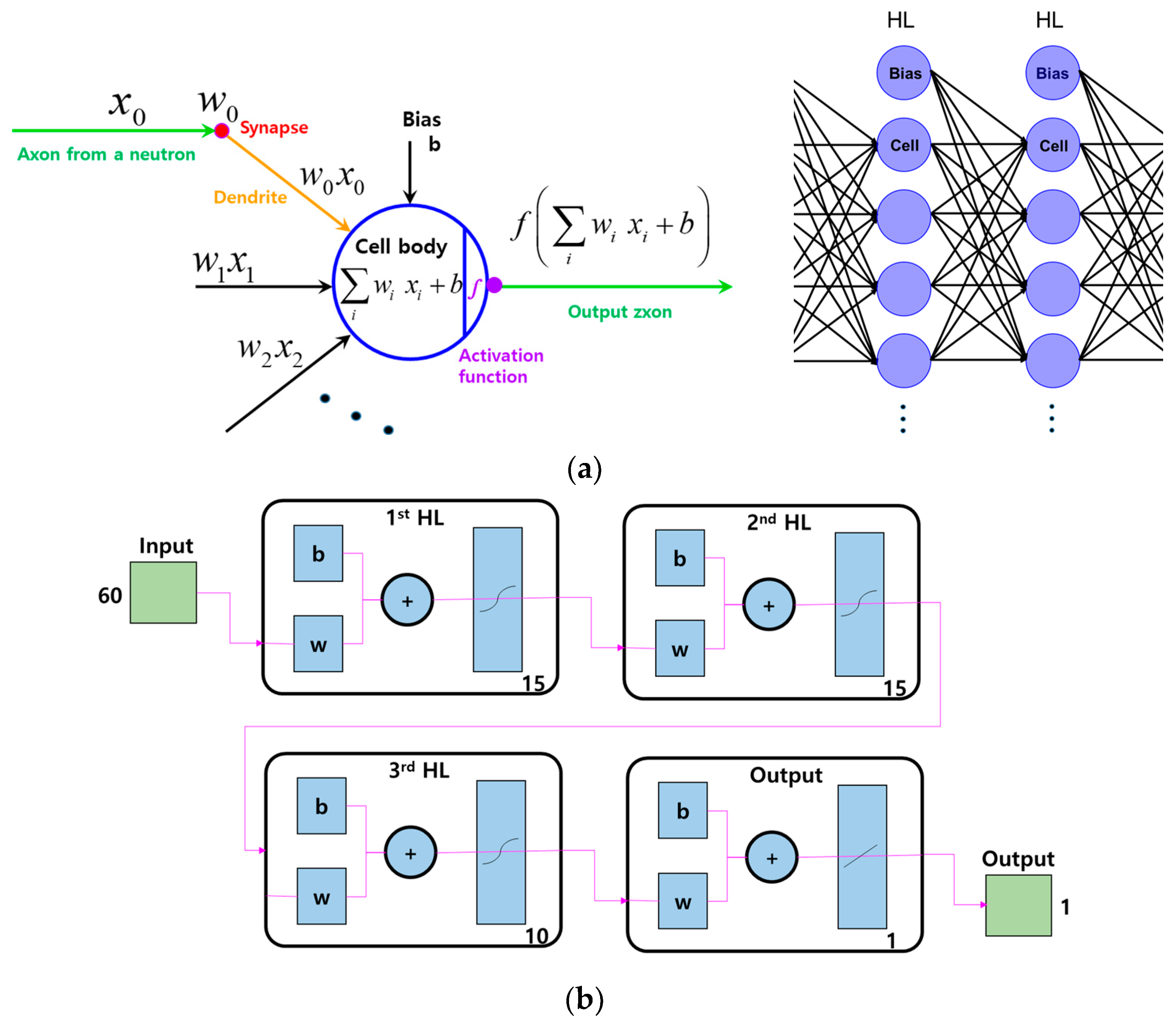
As the typical architectural details of the MLP, this study used 3 hidden layers, used 60 time step delays for each feature, and set the prediction range to 40. The mathematical model of a biological neuron, along with a simple MLP architecture, is depicted in Figure 2a. Regarding the structural details of the MLP, it comprises three hidden layers with 15, 15, and 10 neurons, respectively. The rectified linear unit (ReLU) activation function was utilized. The maximum number of iterations is set to 100, and a dropout with a probability of 0.5 is applied to the hidden layer to avoid overfitting. MSE is used as the error metrics for model training, and an Adam optimizer (adaptive momentum optimizer) is used to update the weights. In total, 80% of the dataset was used for training, with 10% for validation, and 10% for testing. The software package used is Matlab R2022b from Mathworks. Figure 2b shows the MLP architecture used.
There are various ways to compare and evaluate the performance of deep learning architectures, but in this study, error indicators of R2, RMSE, and MAE, and other abbreviations were used and defined as follows [6].
R 2 = 1 i = 1 n y f o r e c a s t i n g , i y o b s e r v e d , i 2 i = 1 n y f o r e c a s t i n g , i y ¯ o b s e r v e d , i 2
R M S E = i = 1 m y i y ^ i 2 m
M A E = 1 m i = 1 m y i y ^ i 2
M A P E = 1 n i = 1 n y f o r e c a s t i n g , i y o b s e r v e d , i y o b s e r v e d , i × 100
M S E = 1 n i = 1 n y f o r e c a s t i n g , i y o b s e r v e d , i 2
C V R M S E = 1 y ¯ o b s e r v e d   1 n i = 1 n y f o r e c a s t i n g , i y o b s e r v e d , i 2   × 100
M B E = 1 n i = 1 n y f o r e c a s t i n g , i y o b s e r v e d , i
N M B E = 1 n i = 1 n y f o r e c a s t i n g , i y o b s e r v e d , i y ¯ o b s e r v e d × 100
M R E = y ¯ f o r e c a s t i n g , i y ¯ o b s e r v e d , i y ¯ o b s e r v e d , i
where y f o r e c a s t i n g and y o b s e r v e d are the model predicted and actual outputs, respectively, y ¯ is the average of the outputs, and n is the number of samples.

3. Results and Discussion

3.1. Data Analysis

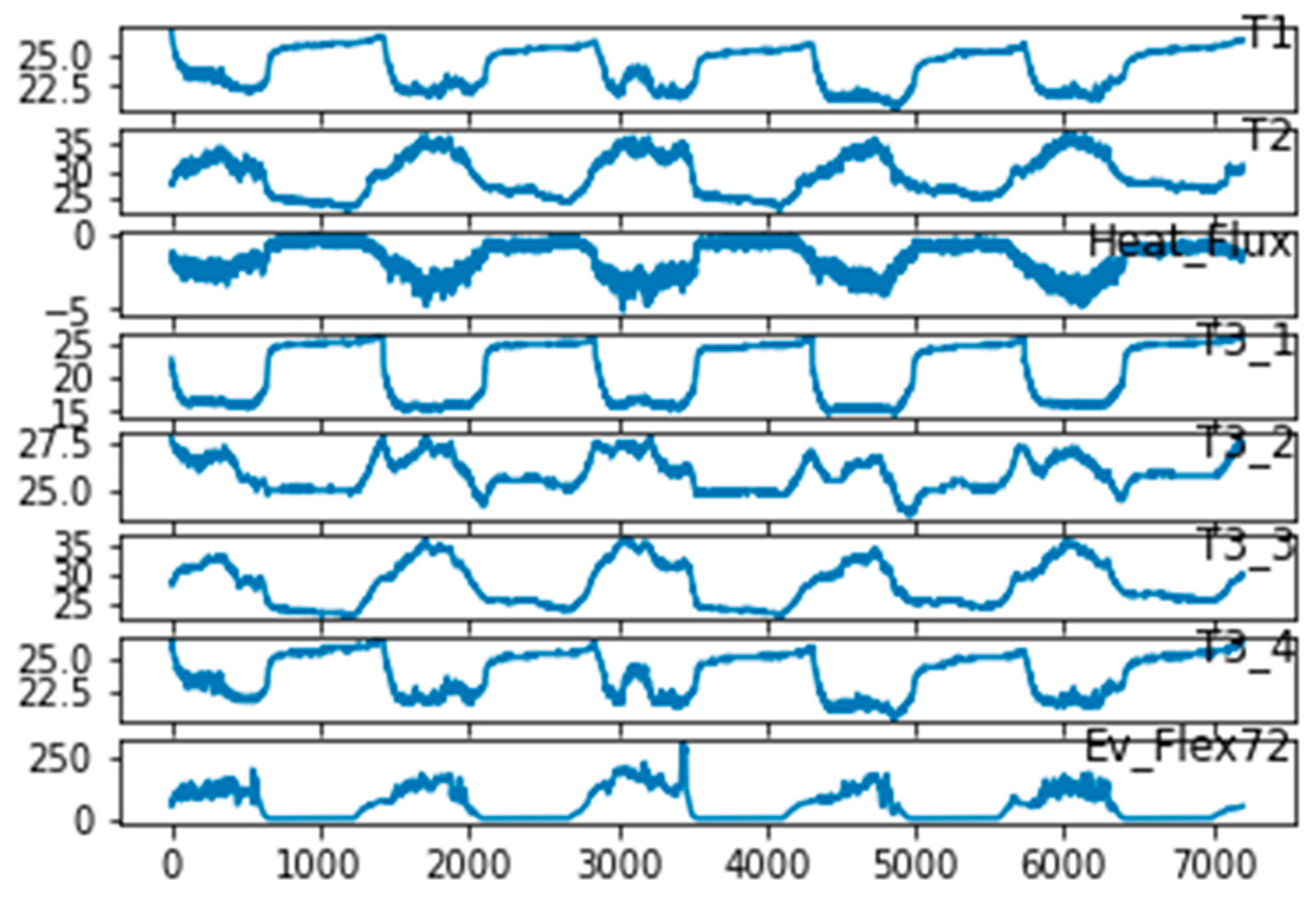
Data on artificial neural networks were measured in a test room around mid-July of this year. The measured data were integrated to construct a 432,000 × 8 feature matrix. Detailed information on the measured variables and their statistics is summarized in Table 1. The indoor air temperature of the dataset was used as the output variable of the model for prediction. A visualization of these variables is shown in Figure 3.
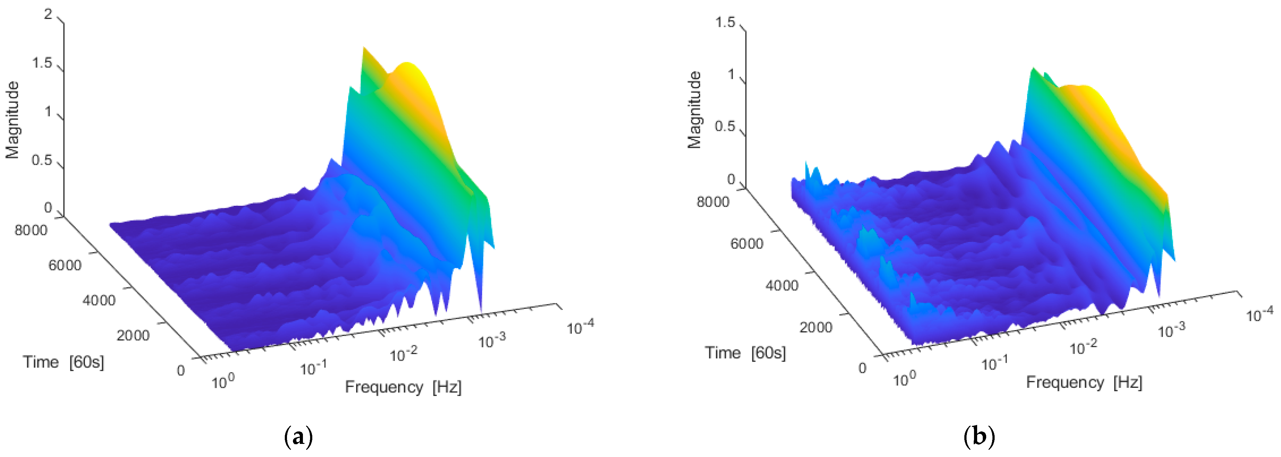
Figure 4 shows the results obtained using wavelet transform to extract and visualize the features from measurements. It is obtained using the analytic Morse wavelet with the symmetry parameter, gamma (γ), equal to 3 and the time-bandwidth product equal to 60 [10,25]. Figure 4a,b show the results of applying wavelet transform on the measured room temperature and heat flux to extract features, respectively. Comparing these two scalograms, it can be observed that the room temperature has a peak at a very low frequency. However, its change over time is quite gentle, and it almost lacks high-frequency components. On the other hand, the heat flux shows significant fluctuations due to the large number of peaks varying not only with time but also with frequency during the weekdays. From these characteristics, useful information can be obtained for the design, operation, and maintenance of control systems for heat load, and their behavior can be easily understood. Using the wavelet transform, it is possible to find characteristics such as indoor temperature, outdoor temperature, window temperature, FCU exit temperature, and window heat flux, so it can be useful for selecting appropriate control variables.

3.2. Artificial Neural Network

The neural network structure used in this study is a multilayer perceptron model and was used to predict indoor temperature. This MLP artificial neural network is trained to predict variables at the next time step using 60 time steps of past data. All performance metrics were evaluated using a test dataset that was not used during training. When multiple time-step predictions are required, the forecasting model iterates the one-step-ahead prediction until the prediction horizon. In general, this process is a closed-loop prediction mechanism that uses current outputs as inputs for predictions at future time steps. A prediction horizon of 40 was used in this study.
Control monitoring time is critical in real plant operation applications. In order to understand the effect of the sampling rate and the number of data, all data were measured at 1 s intervals, and subsampling was used to focus on the effect of the step interval and the number of data. For physical quantity measurement through sensors, 432,000 samples (5 days) were collected for each sensor on weekdays, and multi-level time intervals for subsampling data processing were 1 s, 60 s, 180 s, 300 s, 600 s, 900 s, 1800 s, and 3600 s.
Details of the measured variables and statistics are summarized in Table 1. For the dataset, indoor temperature was used as the target and output variable of the model. The remaining measurements were integrated to construct a 432,000 × 8 feature matrix. A visualization of these remaining variables is shown in Figure 3.
Various error metrics such as R2, RMSE, MAE, and others were calculated for each predicted room temperature. In order to understand the effect of the monitoring and control time interval, modeling was performed according to the sampling rate, and error metrics were compared and shown in Table 2.
Figure 5, Figure 6, Figure 7 and Figure 8 shows the results of training, validation, testing, and prediction for the data subsampled at 180 s time intervals from the data measured by the experimental devices in this study.
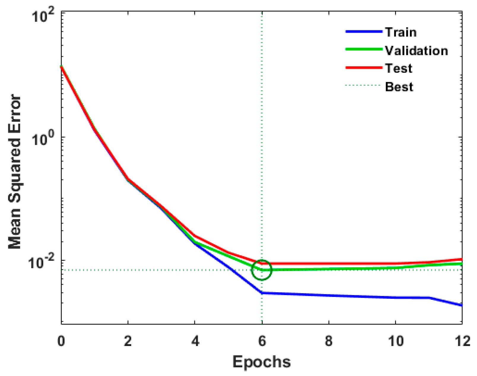
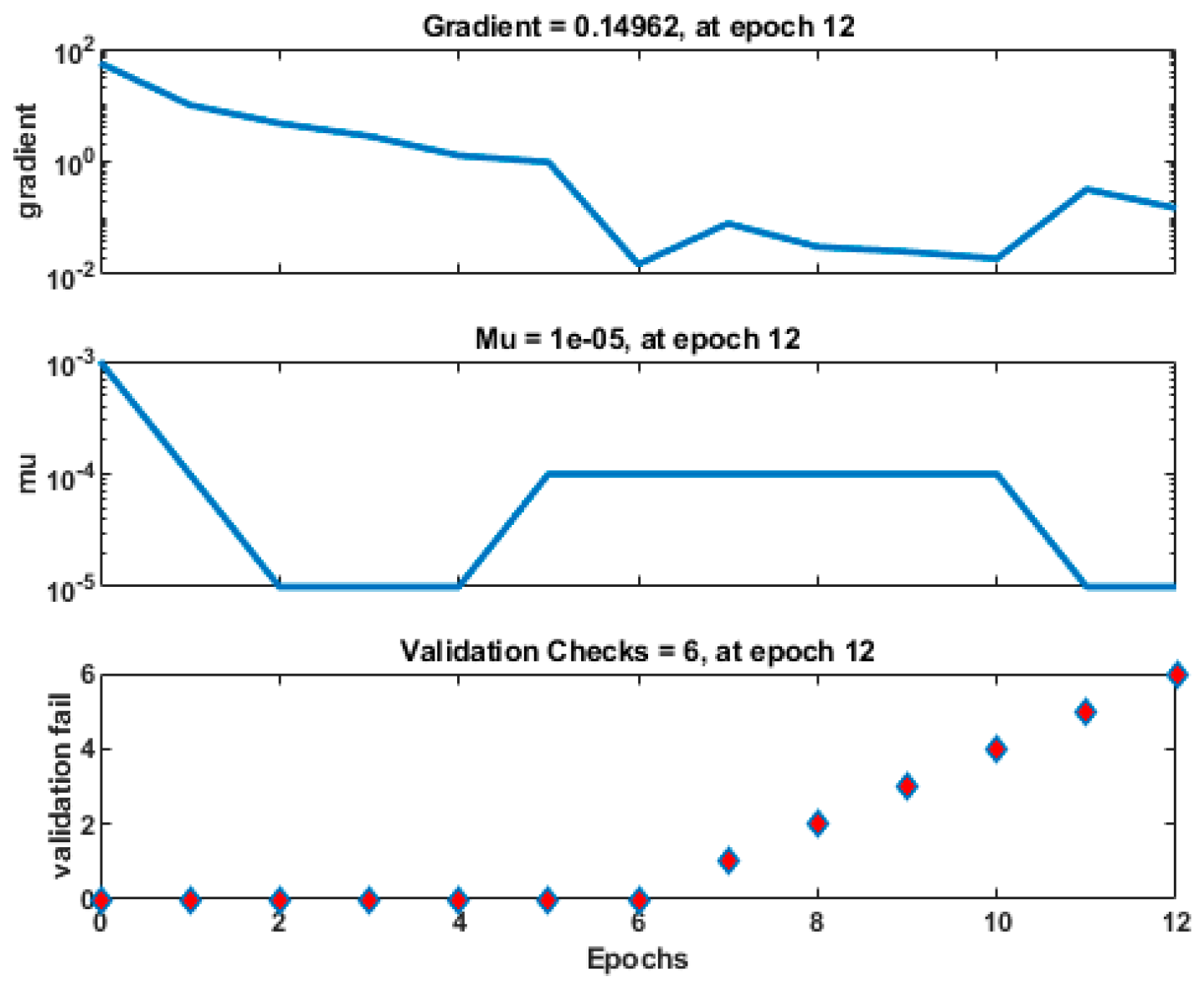
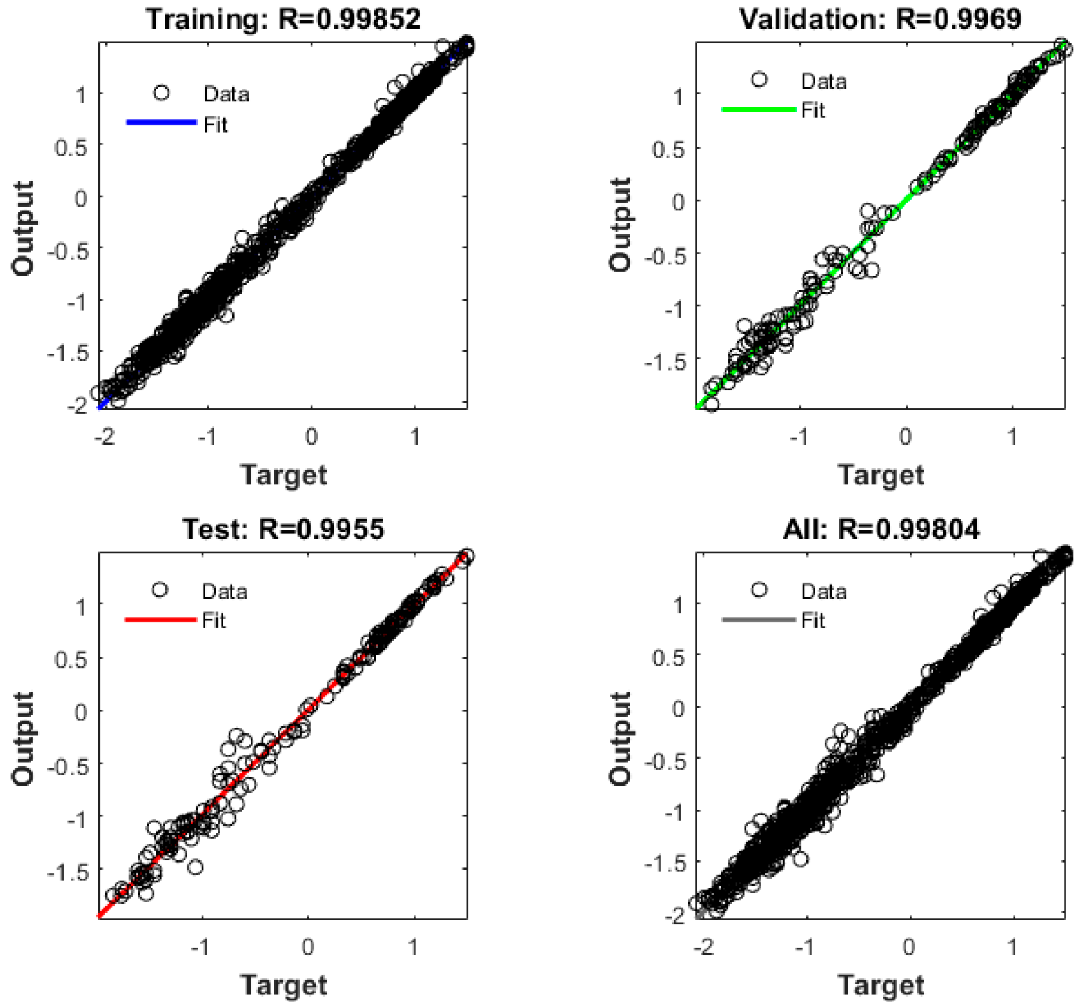
Figure 5 shows the MSE error performance in the process of reaching the maximum epoch 100 in the model using ANN. At the beginning of training, the error rapidly decreased, and when the epoch was 6 or more, the mean square error of the training data was almost constant, and the mean square error of the test dataset was also almost constant, showing a typically excellent predictive tendency [16]. Figure 6 shows the variation in state parameters (gradient, mean, validation failure) according to epochs during the training using ANN model, and the last graph shows that there are six checks that failed validation among 720 validation data. Figure 7 shows the error histogram of the ANN model, and it can be seen that the prediction was successful because there are many data with standard errors close to 0. The ANN model shows very good linearity overall. Figure 8 represents linear regressions of training, validation, test, and all dataset using artificial neural network for tmsi = 180 s and maximum epoch = 100. They all have good linearity.
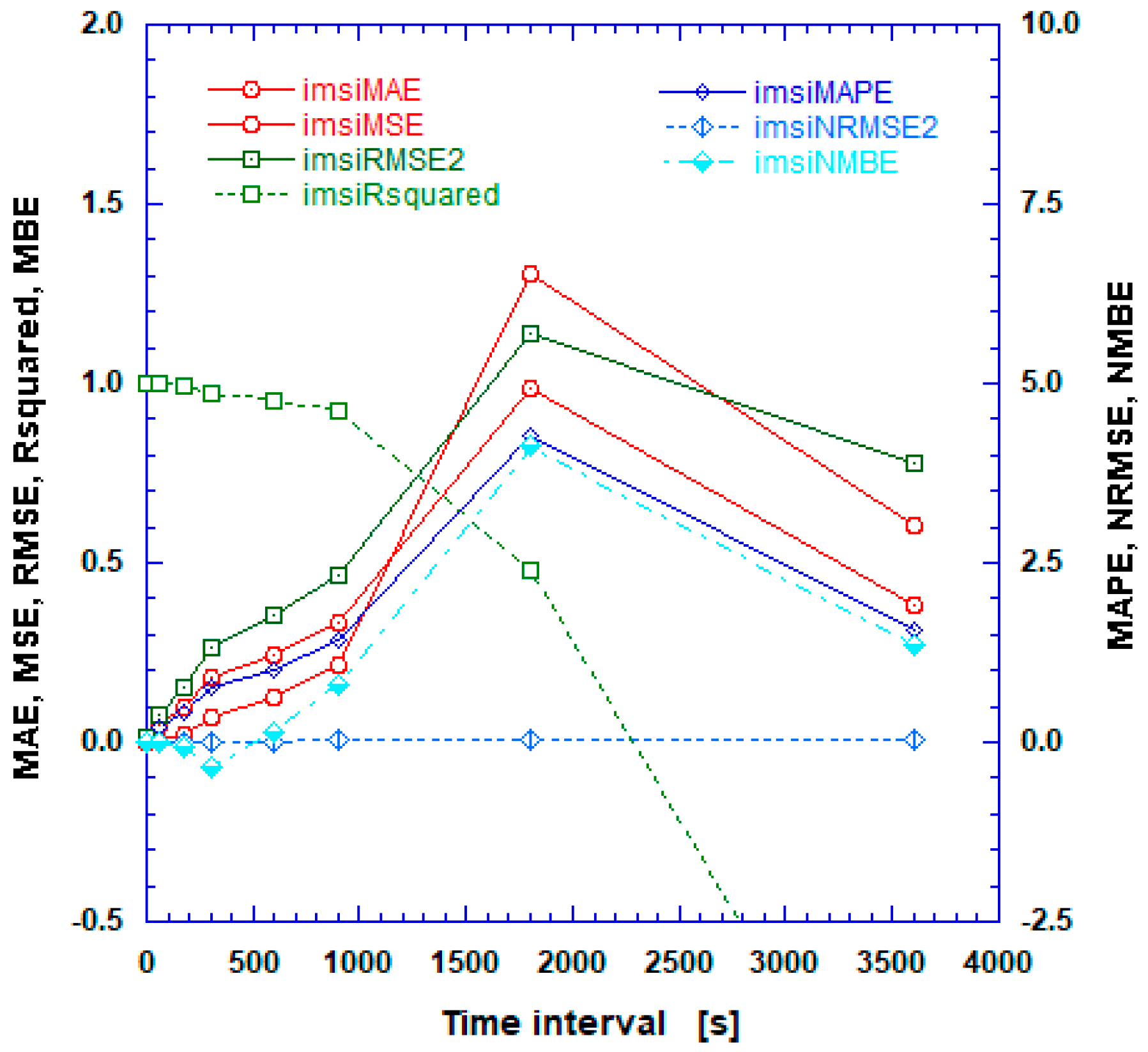
Figure 9 shows various error metrics such as R2, RMSE, and MAE in the model using ANN for subsampling time steps of 1 s, 60 s, 180 s, 300 s, 600 s, 900 s, 1800 s, and 3600 s. Considering the actual operation control mode in which the time interval is important, a comparative analysis was performed accordingly. In addition to the commonly used MSE, MAE, and coefficient of determination (R2), various error indicators in the literature were calculated and trends were compared for reference [10]. Here, looking at the RMSE results, it can be seen that it is desirable to keep the control time interval to 300 s or less because the RMSE value maintains 0.3 or less when the measurement interval of indoor temperature is 300 s or less. When the measurement time interval is longer than 900 s, the RMSE increases rapidly and then decreases at 3600 s. Other performance indicators except SSE, MBE, and NMBE show similar and fairly good trends in this study (See Table 2). A multistep time interval tmsi higher than 900 s is not recommended because the R2 value drops to less than 0.5. Note that it goes to negative unexpectedly at a tmsi of 3600 s. In addition, the computing time is too long at the measurement interval of 1 s, so it is not suitable to use them for control purposes.
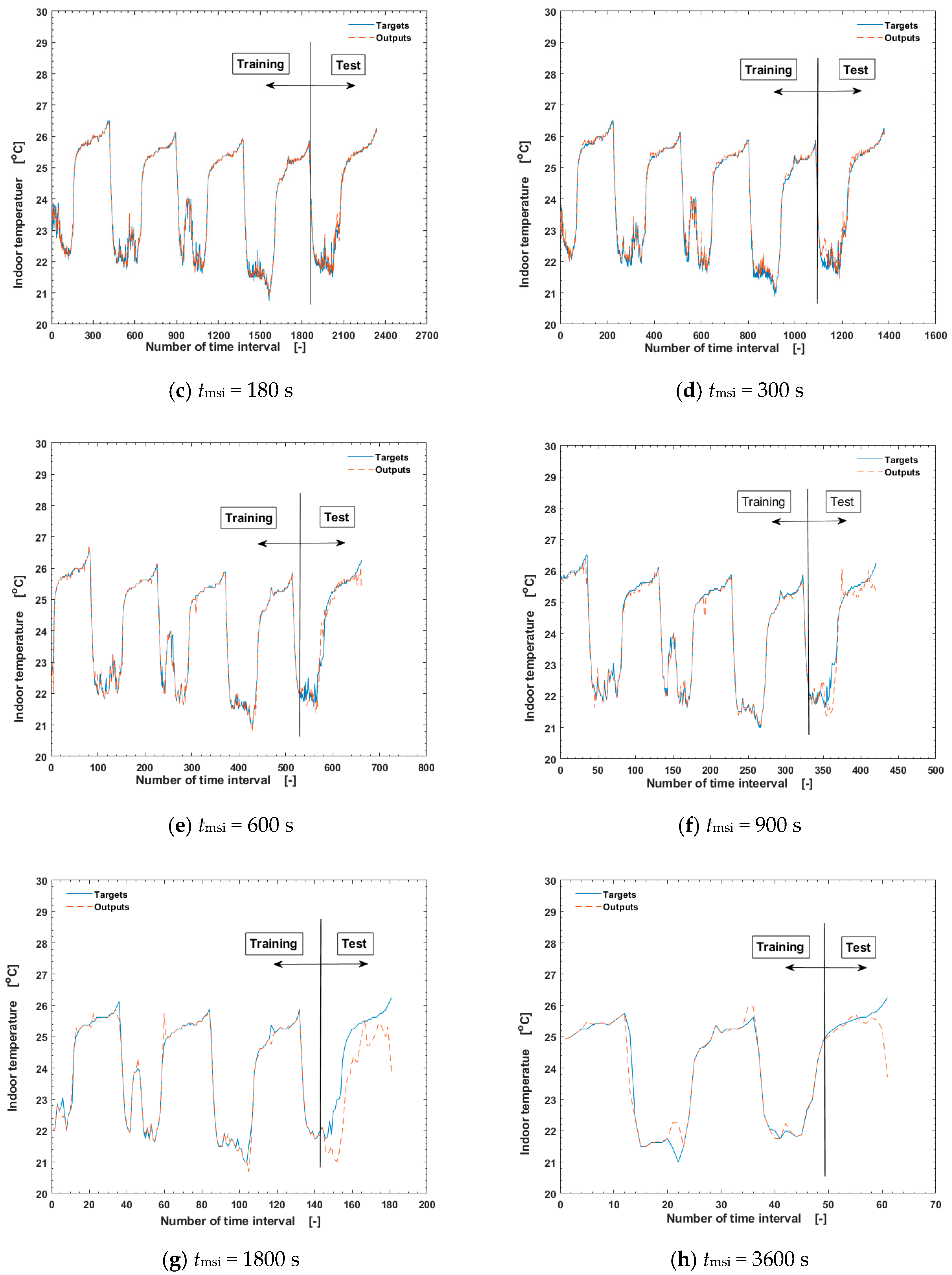
Figure 10 shows the targets and predictions of training and test datasets for each sampling time interval when using the ANN model. In the time interval of 900 s or less, they clearly agree well. And in the time intervals of 1800 s and 3600 s, they show quite plausible behavior except for near the end drop of test outputs. The ANN model had a short computational time compared to other models.
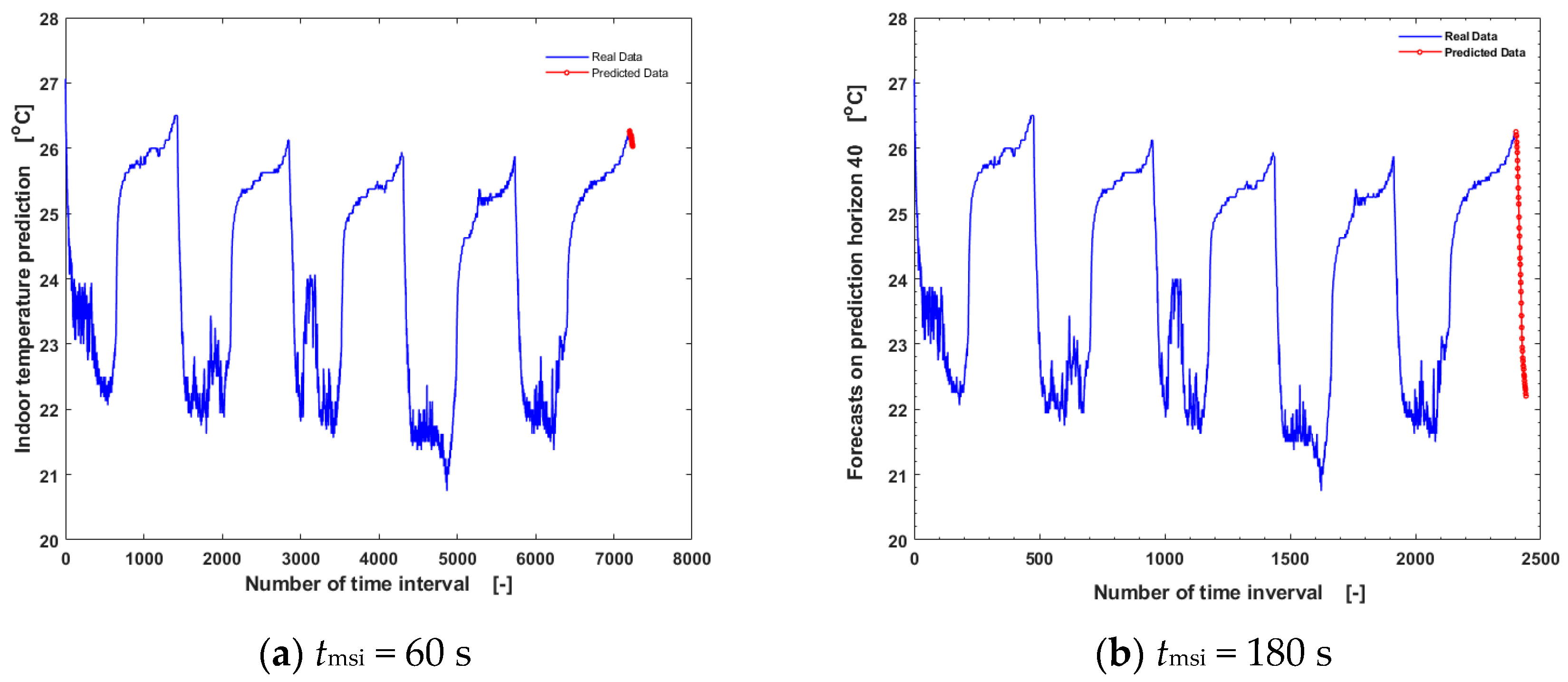
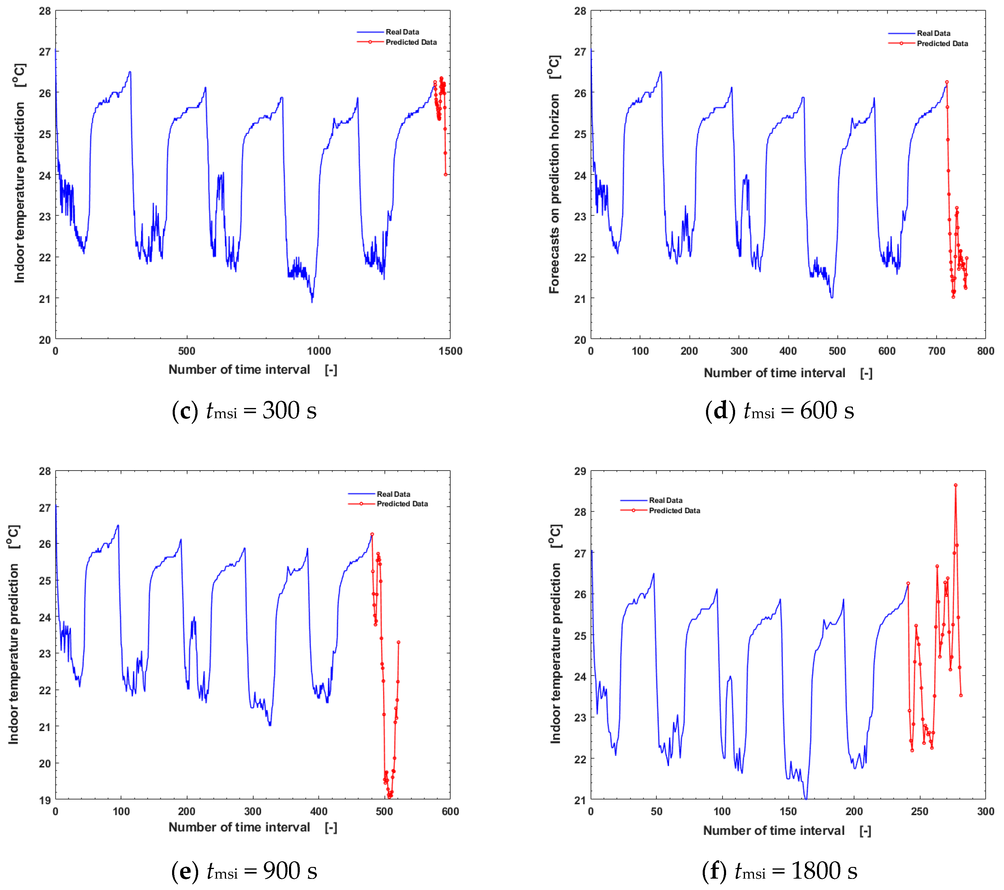
Figure 11 shows the forecasted future indoor temperature in red when the prediction horizon is 40 in the model using ANN. Although the forecasts are subject to change, they provide useful information from a system control point of view. That is, only some of the 40 data points in the prediction horizon can be used as control horizons. We see that indoor temperature has repetitive dynamics with changes in outdoor temperature on weekdays and that previous history has a great influence on future forecasts.
As the multi-step time interval increases, the deviation between the forecast and the measurement accumulates in the next step, similarly to extrapolation [26]. This leads to inevitable performance degradation as the prediction horizon increases. It is advisable to use the results for short-term prediction of the indoor temperature as a guide to decide the appropriate control horizons in the control system. When selecting control horizons for actual operation control from the forecasts or future predictions, it is necessary to comprehensively consider the results of Figure 9 and Figure 10, and the behavior of Figure 11.
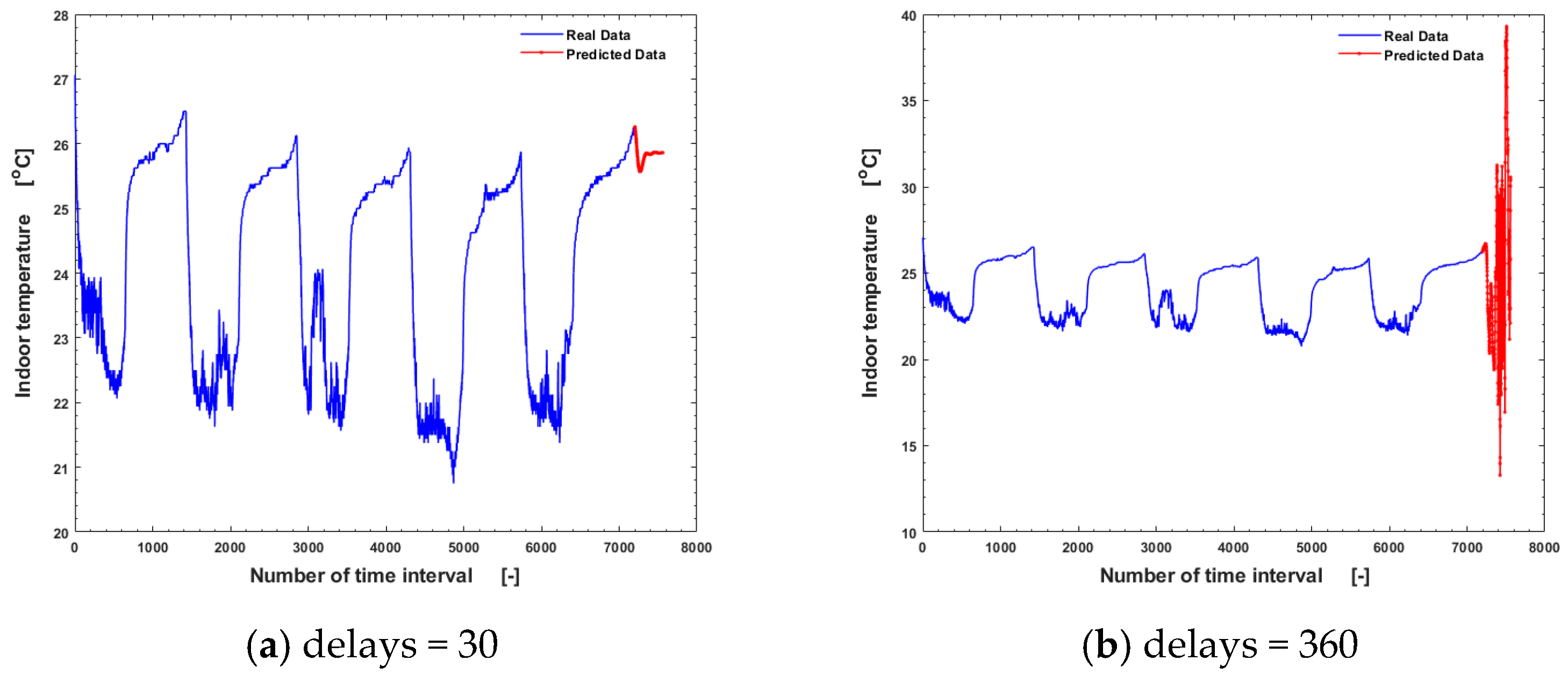
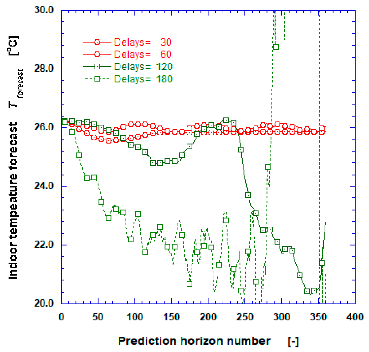
Figure 12 shows the future predictions or forecasts for typical cases where the delays or lags are 30 and 360, respectively, when the tmsi is 60 s. Two typical behaviors of the forecasted indoor temperature are depicted in Figure 12. The red lines in Figure 12a,b are represented by short-term predictions for delays of 30 and 360, respectively. Plausible behavior is exhibited by Figure 12a, while violent oscillations are demonstrated in Figure 12b. From this, it can be seen that the delays significantly impact the results. To examine the effect of these delays on the future predictions more precisely, we obtained the future predictions when the delays changed to 30, 60, 120, and 180 for the case where the multi-step interval tmsi is 60 s and the prediction horizon is 360. The results are compared and presented in Figure 13. To enhance the visibility of the figure, only 10% of the obtained results are marked with symbols. According to the results, when the delays exceed 180, the predicted indoor temperature exhibits large oscillations and becomes unstable. Furthermore, when the delays are below 120 and the prediction horizon number is less than 100, the forecasted indoor temperatures are nearly similar. Namely, if the control horizons are set below 100 for the neural network with an MLP configuration, we can obtain reliable and stable short-term predictions. In short, if the delays are small, the resulting Hankel matrix from time series data is tall and skinny, exhibiting stable characteristics (Figure 12a). However, as the delays increase, the Hankel matrix becomes shallow and wide [9]. This increases calculation time and accumulates errors as the prediction horizon increases, causing instability and large oscillations in temperature calculations (Figure 12b). In other words, when the delays are within a suitable range of input neurons, they exhibit good behavior. For example, prediction and control horizons ranging from 1 to 100 are adopted as tuning parameters when practically implementing model predictive control [24].
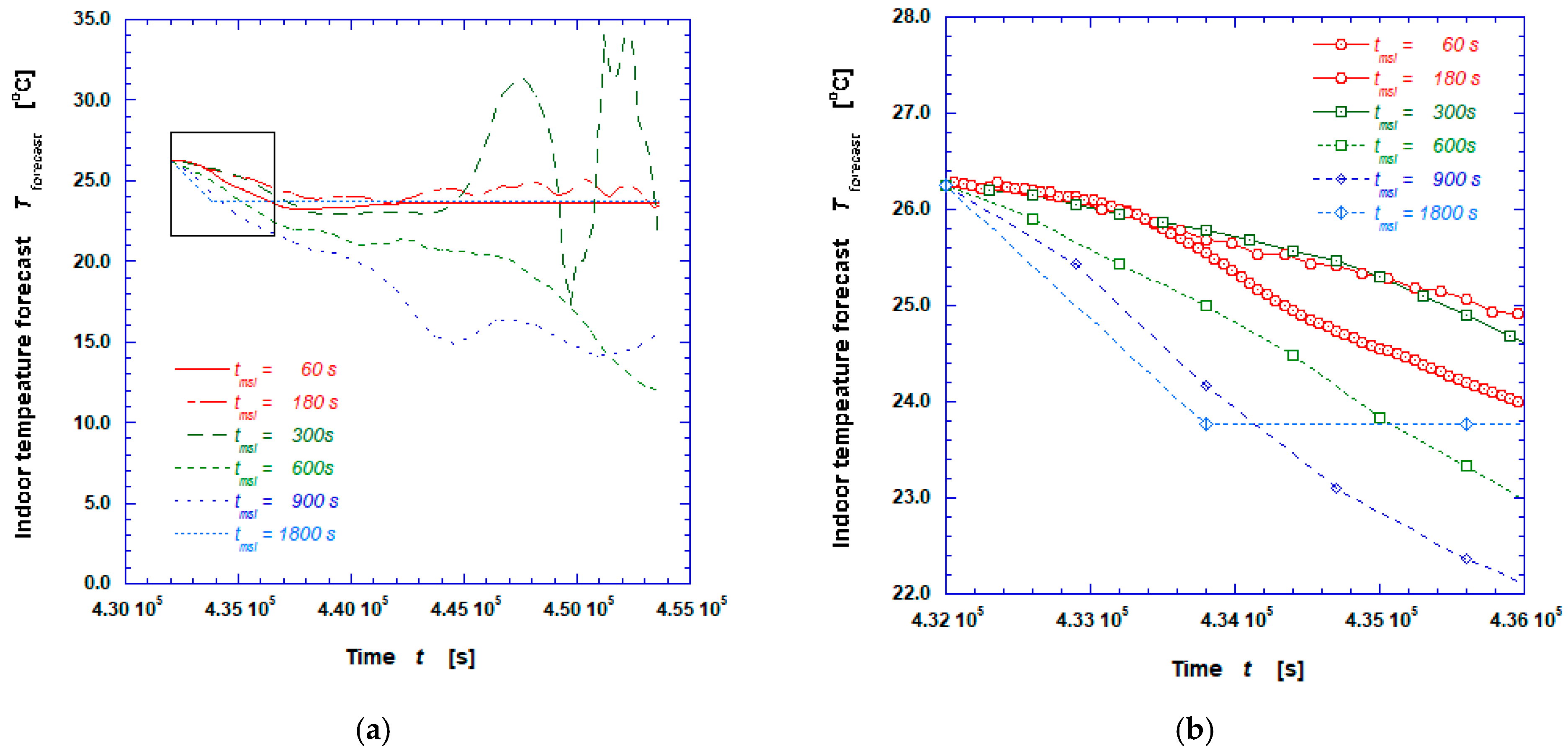
To examine the effect of the multi-step time interval, we predicted the indoor temperature for a duration of 21,600 s, specifically from 432,000 s to 453,600 s (i.e., 360 min), after conducting training, validation, and testing with the delays of 360. The dataset size was adjusted according to the prediction horizons corresponding to the multi-step time interval to make the prediction end time tend = 453,600 s. As can be seen from Figure 14a, the reliability of the short-term predictions or forecasts decreases when the multi-step time interval tmsi = 180 s or more, as large oscillations occur. To examine this in more detail, we enlarged the initial part of the future predictions, shown in Figure 14b, where the symbol marks represent each short-term prediction at each multi-step time interval. From the perspective of short-term control, high reliability was obtained until t = 4.335 × 10⁵ s and at multi-step time intervals tmsi = 300 s or less, as the future predictions are almost identical. Therefore, this gives useful information for the design and configuration of the control system by providing the maximum range of the control horizons according to the multi-step interval.
From the calculated error metrics and the above discussion, it is evident that short-term forecasts using artificial neural networks are highly reliable when tmsi is lower than 300 s, and delays are less than 100. Outside of this range, caution should be exercised for system stability. These results provide useful information to verify the appropriate design and operation in data-driven dynamic control systems or the integration of these with model predictive control. Care must be taken when specifying the indoor air temperature, which may vary for both thermal comfort and energy efficiency, as a control target.

3.3. Multivariate MLP Neural Network Analysis

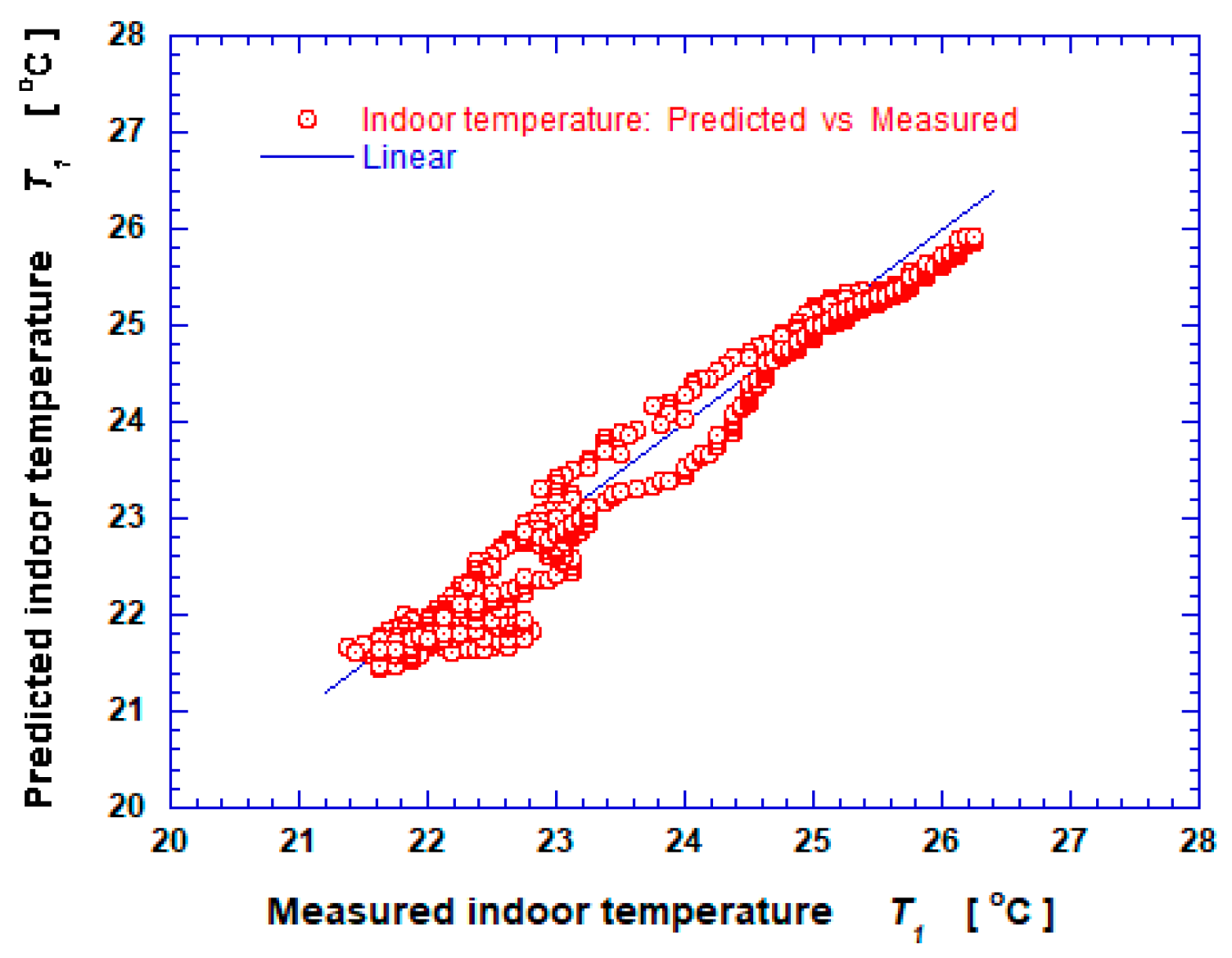
Analyses of a multi-input single-output system (MISO system) were performed considering inputs such as indoor temperature, outdoor temperature, heat flow rate, indoor and outdoor temperatures near the corner of the laboratory, exit air temperature of the fan coil unit (FCU), and indirect illuminance due to solar radiation. The physical quantities presented earlier (refer to Figure 3) were used as input data. Figure 15 shows the time history of measurements and predictions for test data using a multivariate multilayer perceptron neural network model when the multi-step time interval is 60 s. Figure 16 represents the linear regression curve for the multivariate multilayer perceptron model. As before, 80% of the measurement dataset was used for training, 10% for validation, and 10% for testing. An MLP architecture was adopted with a dropout layer (dropout rate of 0.5) to avoid overfitting [27]. In the multivariate model, the calculation time increased considerably compared to a univariate model, and the data dispersion became more severe. Also, as shown in Table 3, the performance index of the multivariate model decreased and worsened compared to the univariate model.
Our future research plans include studies on data-driven dynamic system control, as well as the configuration of data-driven nonlinear dynamic systems in integration with a model predictive controller. At present, we are developing an embedded thermodynamic control system using microcontrollers and signal processing controllers, preparing Matlab and Python programming, and proposing government-funded projects.

4. Conclusions

In this study, the ANN configuration was used to predict the indoor air temperature of a test room with windows on an entire side. Time series data were obtained using sensors and devices in the test room at intervals of 1 s.
Indoor temperature and heat flux features were visualized using wavelet transformation. To investigate the short-term prediction for indoor temperature, we constructed the multilayer perceptron network configurations. They were trained, validated, and tested with the measured datasets. Various error metrics were used and compared to evaluate the performance of the neural network structures. It was shown that the predictions were very successful because the error histogram has data with standard errors close to 0, and the test results have good linearity. The MLP structure has been shown to be useful for the short-term prediction of indoor air temperature. From the comparative analysis performed, the multistep time interval (tmsi) higher than 900 s is not recommended because the R2 value drops to less than 0.5. Short-term forecasts provide useful information from a system control point of view. As the multi-step time interval increases, performance degrades. It is useful to use the results for short-term prediction as a guide to decide the appropriate control horizons in the control system. Among other tuning parameters, delays significantly impact the results. If the control horizons are set below 100 for the MLP configuration investigated in this study, we can obtain reliable and stable short-term predictions. This is because the resulting Hankel matrix from time series data is tall and skinny, exhibiting stable characteristics. Additionally, highly reliable results were obtained at multi-step time intervals (tmsi) of 300 s or less. This also provides useful information for the control horizons in the design of the control system. An increase in the multi-step time interval leads to inevitable performance degradation. Even if the performance of the correlation coefficient progressively worsens as tmsi increases, when tmsi is 180 s or less, the R2 value remains impressively high, exceeding 0.99. A shorter prediction horizon and multiscale time step interval less than 180 s can be used in the control system, which will seem to be reasonable for stability and computational costs. For the multivariate model, the calculation time increased and the data dispersion became more severe. The performance also worsened compared to the univariate model.

Author Contributions

Conceptualization, B.K.P.; data curation, C.-J.K.; formal analysis, B.K.P.; funding acquisition, B.K.P.; investigation, C.-J.K.; methodology, C.-J.K. and B.K.P.; project administration, B.K.P. and C.-J.K.; validation, B.K.P.; writing—original draft B.K.P.; writing—review and editing, C.-J.K. All authors have read and agreed to the published version of the manuscript.

Funding

This research was supported by Ministry of Land, Infrastructure and Transport of the Korean government through Korea Agency for Infrastructure Technology Advancement(KAIA) Grant (No. RS-2021-KA161098).

Data Availability Statement

Data are contained within the article.

Conflicts of Interest

The authors declare no conflict of interest.

Abbreviations

The following abbreviations are used in this manuscript:
AIArtificial intelligence
ANNArtificial neural networks
CNNConvolutional neural network
CVRMSECoefficient of variation of RMSE
FCUFan coil unit
LSTMLong short-term memory
MLPMultilayer perceptron
MPCModel predictive controller
MAEMean absolute error
MAPEMaximum absolute percent error
MBEMean bias error
MREMean relative error
MSEMean squared error
NMBENormalized MBE
NRMSENormalized RMSE
RMSERoot mean square error
RMSPERoot mean square percentage error
SSESum squared error

References

  1. International Energy Agency. Energy Systems, Buildings. Available online: https://www.iea.org/energy-system/buildings (accessed on 19 September 2023).
  2. Tafakkori, R.; Fattahi, A. Introducing novel configurations for double-glazed windows with lower energy loss. Sustain. Energy Technol. Assess. 2021, 43, 100919. [Google Scholar] [CrossRef]
  3. ASHRAE. Handbook Fundamentals, SI, International Edition, 1997; ASHRAE Handbook—HVAC Applications; ASHRAE Parsons: Peachtree Corners, GA, USA, 2007.
  4. Lu, C.; Li, S.; Lu, Z. Building energy prediction using artificial neural networks: A literature survey. Energy Build. 2021, 262, 111718. [Google Scholar] [CrossRef]
  5. Wang, Z.; Chen, Y. Data-driven modeling of building thermal dynamics: Methodology and state of the art. Energy Build. 2019, 203, 109405. [Google Scholar] [CrossRef]
  6. Bourdeau, M.; Zhai, X.Q.; Nefzaoui, E.; Guo, X.; Chatellier, P. Modeling and forecasting building energy consumption: A review of data-driven techniques. Sustain. Cities Soc. 2019, 48, 101533. [Google Scholar] [CrossRef]
  7. Kirubakaran, V.; Sahu, C.; Radhakrishnan, T.; Sivakumaran, N. Energy efficient model based algorithm for control of building HVAC systems. Ecotoxicol. Environ. Saf. 2015, 121, 236–243. [Google Scholar] [CrossRef] [PubMed]
  8. Ming, W.; Sun, P.; Zhang, Z.; Qiu, W.; Du, J.; Li, X.; Zhang, Y.; Zhang, G.; Liu, K.; Wang, Y.; et al. A systematic review of machine learning methods applied to fuel cells in performance evaluation, durability prediction, and application monitoring. Int. J. Hydrogen Energy 2023, 48, 5197–5228. [Google Scholar] [CrossRef]
  9. Brunton, S.L.; Kutz, J.N. Data-Driven Science and Engineering—Machine Learning, Dynamical Systems, and Control, 2nd ed.; Cambridge University Press: Cambridge, UK, 2022. [Google Scholar]
  10. Park, B.K.; Cho, D.W.; Shin, H.J. Energy Analysis for Variable Air Volume System. Mag. Soc. Air-Cond. Refrig. Eng. Korea 1988, 17, 575–582. [Google Scholar]
  11. Roman, N.D.; Bre, F.; Fachinotti, V.D.; Lamberts, R. Application and characterization of metamodels based on artificial neural networks for building performance simulation: A systematic review. Energy Build. 2020, 217, 109972. [Google Scholar] [CrossRef]
  12. Tien, P.W.; Wei, S.; Darkwa, J.; Wood, C.; Calautit, J.K. Machine Learning and Deep Learning Methods for Enhancing Building Energy Efficiency and Indoor Environmental Quality—A Review. Energy AI 2022, 10, 100198. [Google Scholar] [CrossRef]
  13. Chen, Z.; Xiao, F.; Guo, F.; Yan, J. Interpretable machine learning for building energy management: A state-of-the-art review. Adv. Appl. Energy 2023, 9, 100123. [Google Scholar] [CrossRef]
  14. Noye, S.; Martinez, R.M.; Carnieletto, L.; DeCarli, M.; Aguirre, A.C. A review of advanced ground source heat pump control: Artificial intelligence for autonomous and adaptive control. Renew. Sustain. Energy Rev. 2022, 153, 111685. [Google Scholar] [CrossRef]
  15. Bellagarda, A.; Cesari, S.; Aliberti, A.; Ugliotti, F.; Bottaccioli, L.; Macii, E.; Patti, E. Effectiveness of neural networks and transfer learning for indoor air-temperature forecasting. Autom. Constr. 2022, 140, 104314. [Google Scholar] [CrossRef]
  16. Attoue, N.; Shahrour, I.; Younes, R. Smart Building; Use of the Artificial Neural Network Approach for Indoor Temperature Forecasting. Energies 2018, 11, 395. [Google Scholar] [CrossRef]
  17. Kreuzer, D.; Munz, M.; Schlüter, S. Short-term temperature forecasts using a convolutional neural network—An application to different weather stations in Germany. Mach. Learn. Appl. 2020, 2, 100007. [Google Scholar] [CrossRef]
  18. Xu, C.; Chen, H.; Wang, J.; Guo, Y.; Yuan, Y. Improving prediction performance for indoor temperature in public buildings based on a novel deep learning method. Build. Environ. 2019, 148, 128–135. [Google Scholar] [CrossRef]
  19. Kamel, E.; Javan-Khoshkholgh, A.; Abumahfouz, N.; Huang, S.; Huang, X.; Farajidavar, A.; Qiu, Y. A case study of using multi-functional sensors to predict the indoor air temperature in classrooms. ASHRAE Trans. 2020, 26, 3–11. [Google Scholar]
  20. Aliberti, A.; Bottaccioli, L.; Macii, E.; Cataldo, S.D.; Acquaviva, A.; Patti, E. A non-linear autoregressive model for indoor air-temperature predictions in smart buildings. Electronics 2019, 8, 979. [Google Scholar] [CrossRef]
  21. Cifuentes, J.; Marulanda, G.; Bello, A.; Reneses, J. Air temperature forecasting using machine learning techniques: A review. Energies 2020, 13, 4215. [Google Scholar] [CrossRef]
  22. Park, B.K.; Kim, C.-J. Unsteady Heat Flux Measurement and Predictions Using Long Short-Term Memory Networks. Buildings 2023, 13, 707. [Google Scholar] [CrossRef]
  23. Pawar, P.; Kumar, M.T.; Vittal, K.P. An IoT based Intelligent Smart Energy Management System with accurate forecasting and load strategy for renewable generation. Measurement 2020, 152, 107187. [Google Scholar] [CrossRef]
  24. Schwenzer, M.; Ay, M.; Bergs, T.; Dirk Abel, D. Review on model predictive control: An engineering perspective. Int. J. Adv. Manuf. Technol. 2021, 117, 1327–1349. [Google Scholar] [CrossRef]
  25. Mathlab. Deep Learning Toolbox; Mathoworks: Natick, MA, USA, 2022. [Google Scholar]
  26. Chapra, S.C.; Canale, R.P. Numerical Method for Engineers, 4th ed.; McGraw Hill: New York, NY, USA, 2002. [Google Scholar]
  27. Brownlee, J. Deep Learning for Time Series Forecasting—Predict the Future with MLPs, CNNs, and LSTMs in Python; Machine Learning Mastery: San Juan, PR, USA, 2020. [Google Scholar]
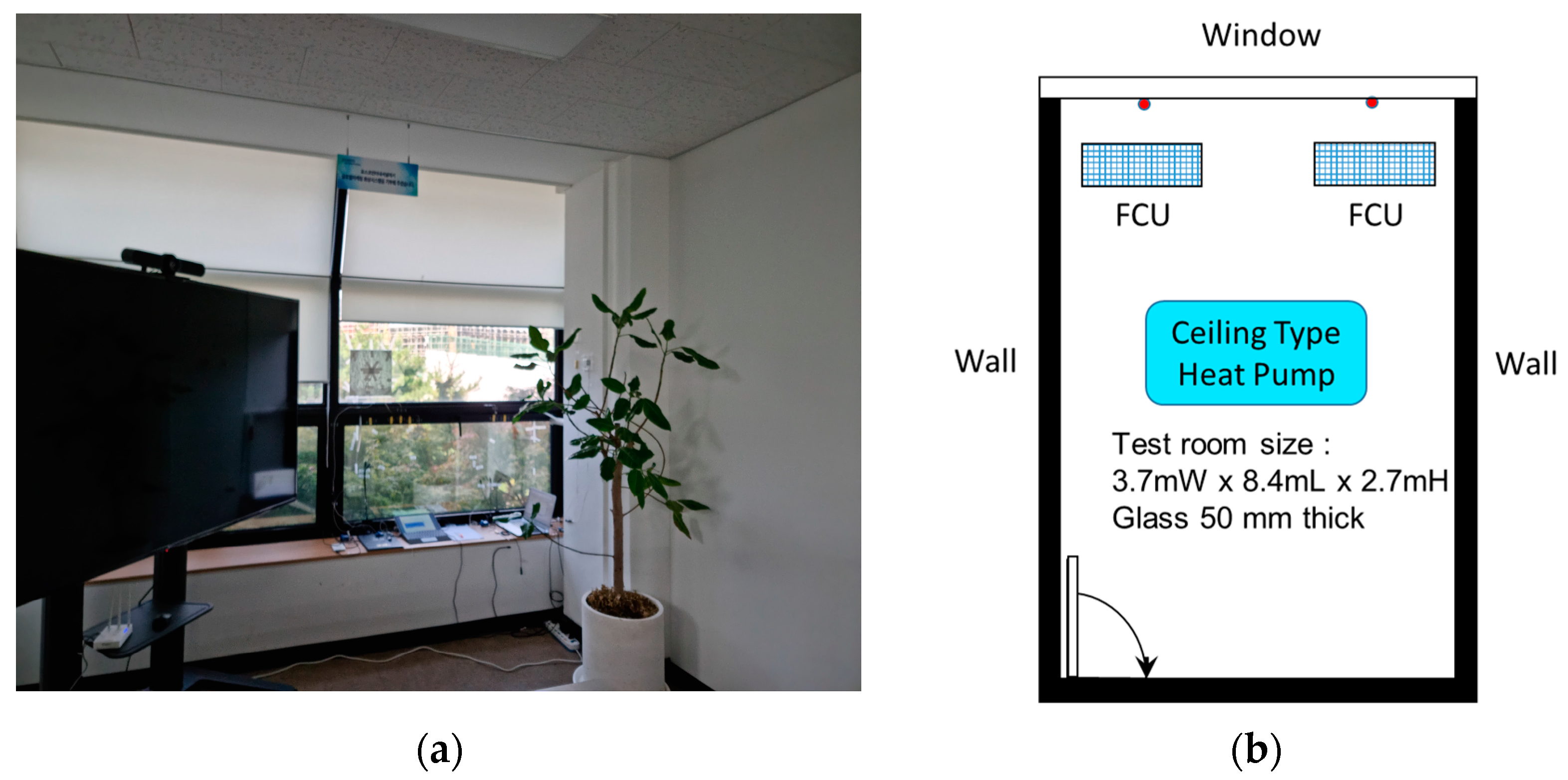
Figure 1. Photograph (a) and schematic (b) of the test room.
Energies 16 07724 g001
Figure 2. Schematic of (a) a node model and hidden layers and (b) the MLP architecture. HL stands for Hidden Layer.
Energies 16 07724 g002
Figure 3. Visualization of dataset for artificial neural network analysis.
Energies 16 07724 g003
Figure 4. Three dimensional scalogram for (a) indoor temperature and (b) heat flux.
Energies 16 07724 g004
Figure 5. Artificial neural network performance (maximum epoch = 100; tmsi = 180 s).
Energies 16 07724 g005
Figure 6. Variations in state parameters during ANN training (maximum epoch = 100; tmsi = 180 s).
Energies 16 07724 g006
Figure 7. Error histogram using artificial neural network prediction (maximum epoch = 100, tmsi = 180 s).
Energies 16 07724 g007
Figure 8. Regression using artificial neural network for training, validation, test, and all data (maximum epoch = 100, tmsi = 180 s).
Energies 16 07724 g008
Figure 9. Performance index comparison for ANN architecture (test dataset, indoor temperature).
Energies 16 07724 g009
Figure 10. Output graph evaluation for all data (MLP model).
Energies 16 07724 g010aEnergies 16 07724 g010b
Figure 11. Forecasts (future predictions) on horizon 40; forecast using MLP model (prediction horizon: 40). Red symbols indicate short-term predictions (forecasts) for control.
Energies 16 07724 g011aEnergies 16 07724 g011b
Figure 12. Typical forecasts (near-future predictions) using MLP model (tmsi: 60 s; prediction horizon: 360). Red lines indicate short-term predictions (forecasts) for control. Blue lines indicate measured real data.
Energies 16 07724 g012
Figure 13. Effects of delays on forecasts. Symbols indicate only the 10% of forecasts for clarity (tmsi: 60 s; prediction horizon: 360).
Energies 16 07724 g013
Figure 14. Effects of multistep time interval on forecasts: (a) forecasts from 43,200 s to 453,600 s; (b) zoomed-in view of box in (a), at very short time horizons (tmsi: 60 s). Symbols in (b) indicate short-term predictions (forecasts).
Energies 16 07724 g014
Figure 15. Output graph evaluation for test data in the multivariate MLP model (tmsi = 60 s).
Energies 16 07724 g015
Figure 16. Regression for test data in the multivariate MLP model (tmsi = 60 s).
Energies 16 07724 g016
Table 1. Statistical summary of the dataset.
MinimumMaximumMeanStandard Dev.
T1 (Indoor temp.)20.7527.0624.091.61
T2 (Outdoor temp.)22.943729.023.58
Heat_Flux (Heat flux)−5.12−0.04−1.641.04
T3_1 (FCU outlet temp.)14.7526.2520.964.31
T3_2 (Pane inside temp.)23.7527.7525.840.85
T3_3 (Pane outside temp.)233628.223.67
T3_4 (Indoor temp. 2)20.526.2523.811.59
Ev_Flex72 (Illuminance)0.13316.857.8162.37
Table 2. Calculated error metric for various multi-step time intervals in test data (Tindoor, MLP).
tmsi [s]R2RMSEMAEMAPEMSENRMSECVRMSESSEMBENMBE
10.9999070.0158530.0069260.0289270.0002510.0006600.32335621.709646−0.000289−0.001201
600.9976920.0794490.0490320.2153870.0063120.0033061.6206679.0136490.0020190.008402
1800.9912360.1550630.0941410.4097500.0240440.0064483.16092511.252788−0.017319−0.071967
3000.9735760.2611090.1783040.7689510.0681780.0108475.31246218.817129−0.085975−0.355893
6000.9531700.3530700.2404781.0219330.1246580.0146077.18617516.4548860.0325370.134789
9000.9218780.4632060.3302181.4144340.2145600.0190759.43680418.0230090.1900810.788933
18000.4799171.1423410.9872494.2637001.3049440.04621023.44729546.9779750.9845544.147949
3600−1.3120620.7770900.3848121.5750310.6038680.03034415.4587377.2464190.3400191.345580
Table 3. Comparison of performance evaluation of the MLP model for test data (tmsi = 60 s).
R2RMSEMAEMAPEMSECVRMSESSEMBENMBEMRE
MLP (univariate)0.9980.0790.0490.2150.0061.6209.0130.0020.0088.4 × 10−5
MLP (multivariate)0.9740.2640.2240.9330.0695.359102.03−0.197−0.8170.008
Disclaimer/Publisher’s Note: The statements, opinions and data contained in all publications are solely those of the individual author(s) and contributor(s) and not of MDPI and/or the editor(s). MDPI and/or the editor(s) disclaim responsibility for any injury to people or property resulting from any ideas, methods, instructions or products referred to in the content.