
Estimating Compressional Velocity and Bulk Density Logs in Marine Gas Hydrates Using Machine Learning


Abstract
:1. Introduction
2. Data
2.1. Training Holes
2.2. Test Holes
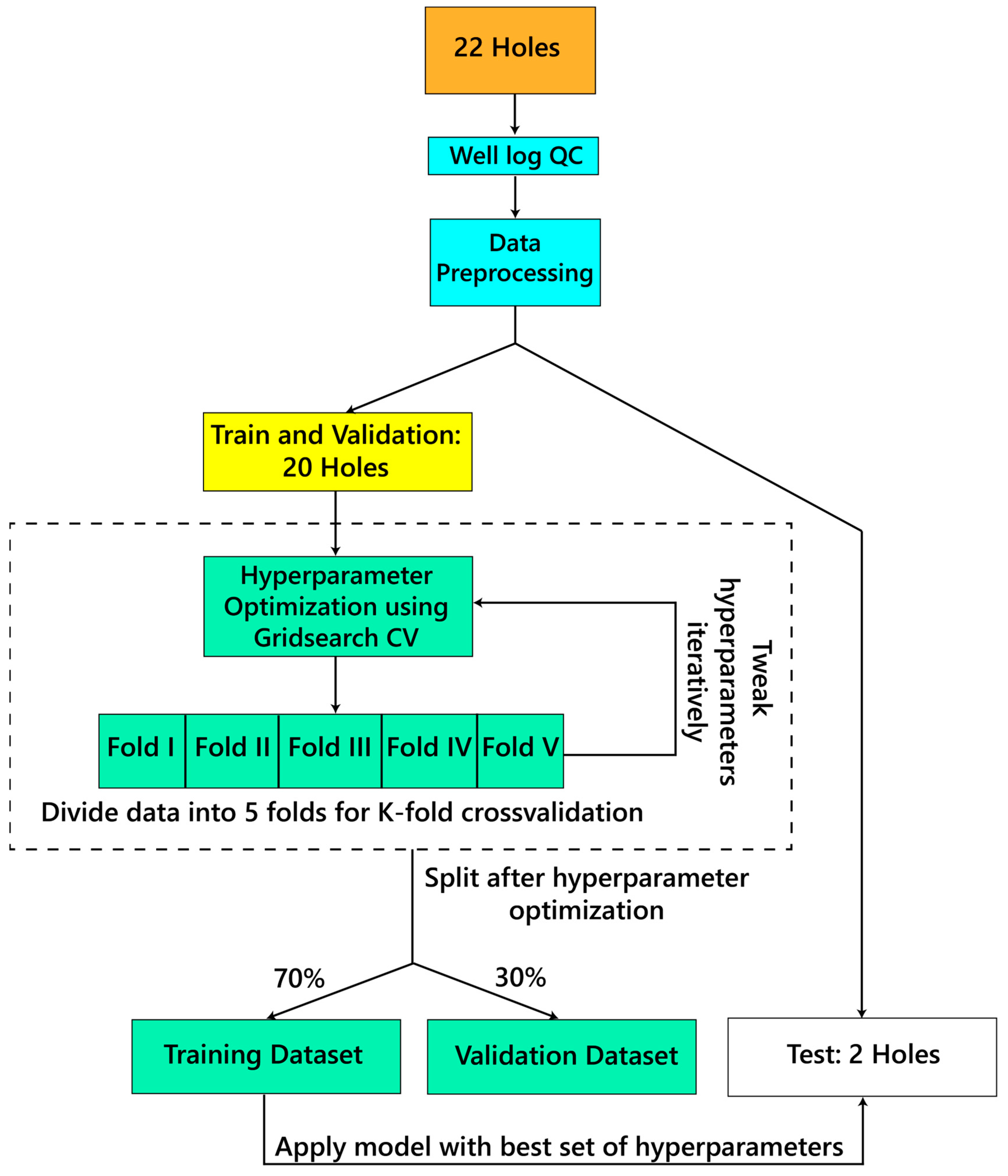
3. Methods
3.1. Machine Learning Algorithms
- a.
- Multilinear Regression: Multilinear regression develops a correlation between the provided inputs and outputs on a labeled training dataset using a linear relationship, and the resulting linear model is used to predict values for a new dataset [53]. This algorithm does not require hyperparameter tuning.
- b.
- Polynomial Regression: This algorithm defines a relationship between the input and output parameters based on an nth-degree polynomial. The user defines the degree of the polynomial, and then, the algorithm transforms the input data into a polynomial equation [54]. For a supervised learning model, the same equation is then used to predict outputs based on a novice dataset. Herein, we tested polynomial equations from orders two to six and chose a 4th order polynomial equation after hyperparameter tuning.
- c.
- Polynomial Regression with Ridge Regularization (L2): L2 regularization reduces overfitting by adding a penalty term that can be used to reduce the magnitude of large coefficients in the equation [55]. Here, we combine a 4th-order polynomial equation with a ridge regression fit on the training data. We use regularization values of 0.001 and 0.01 to predict Vp and ρb, respectively.
- d.
- K Nearest Neighbors: This algorithm uses feature similarity between input and output points in a space to make predictions [16]. Whenever a new dataset is input into the model, the Euclidean distance from the training data points is calculated for all the new data points, and then, the nearest neighboring values are selected based on the k value, which defines the search criteria and selects k nearest neighbors from the input (e.g., [16]). Another parameter, the weight attribute, weighs different points in the neighborhood corresponding to their respective Euclidean distances. The closeness that is calculated as the Euclidean distance from training points is then used to predict an output based on the class of the nearest neighbors [56]. We select k = 7 and ‘distance’ as the weight attribute as they fit the model best for predicting Vp and ρb.
- e.
- Random Forest: As described in [57] and other research works in geosciences such as Bressan et al., Hou et al., and Shalaby et al. [20,22,25], random forest uses a bootstrap aggregating method that uses a combination of decision trees and takes the mean out of all the decision trees to generate the final output. Decision trees mimic the structure of a tree and consist of several nodes that terminate on a leaf node [58]. Leaf nodes are representative of class labels, and all other nodes signify feature attributes. Each branch of the tree used in random forest is subdivided into nodes based on the conditions that the algorithm tries to construct with reference to the input data provided [58]. This structure of random forest reduces variance and avoids overfitting. Herein, we use random forest by constructing a forest with ‘400’ trees, ‘sqrt’ as the max_features, which defines the size of the features to be considered while splitting a node; ‘1’ as the min_samples_leaf, which refers to the minimum number of samples at the leaf node; ‘15’ as max_depth, which refers to the maximum depth of the tree from the root node to the leaf node; and ‘2’ as the min_samples_split, which refers to the minimum number of samples required to split a node.
- f.
- Multilayer Perceptron: A multilayer perceptron is an artificial neural network that uses artificial neurons with an input layer, a hidden layer, and an output layer to make non-linear predictions based on the inputs provided to it [59]. It is inspired by the structure of biological neurons that receive signals from other neurons via interconnections [60,61]. It has been frequently applied in the geosciences [17,18,19,20,21,22,23,25,27,29,31]. An important part of a multilayer perceptron is the choice of activation function, which defines the output from a neuron. We use the ‘relu’ activation function, which is a piecewise linear function [62], along with four and five hidden layers to predict Vp and ρb, respectively, as it provides the best fit.
3.2. Prediction of ρb and Vp
3.3. Downsampling the Predicted Results
4. Results and Discussion
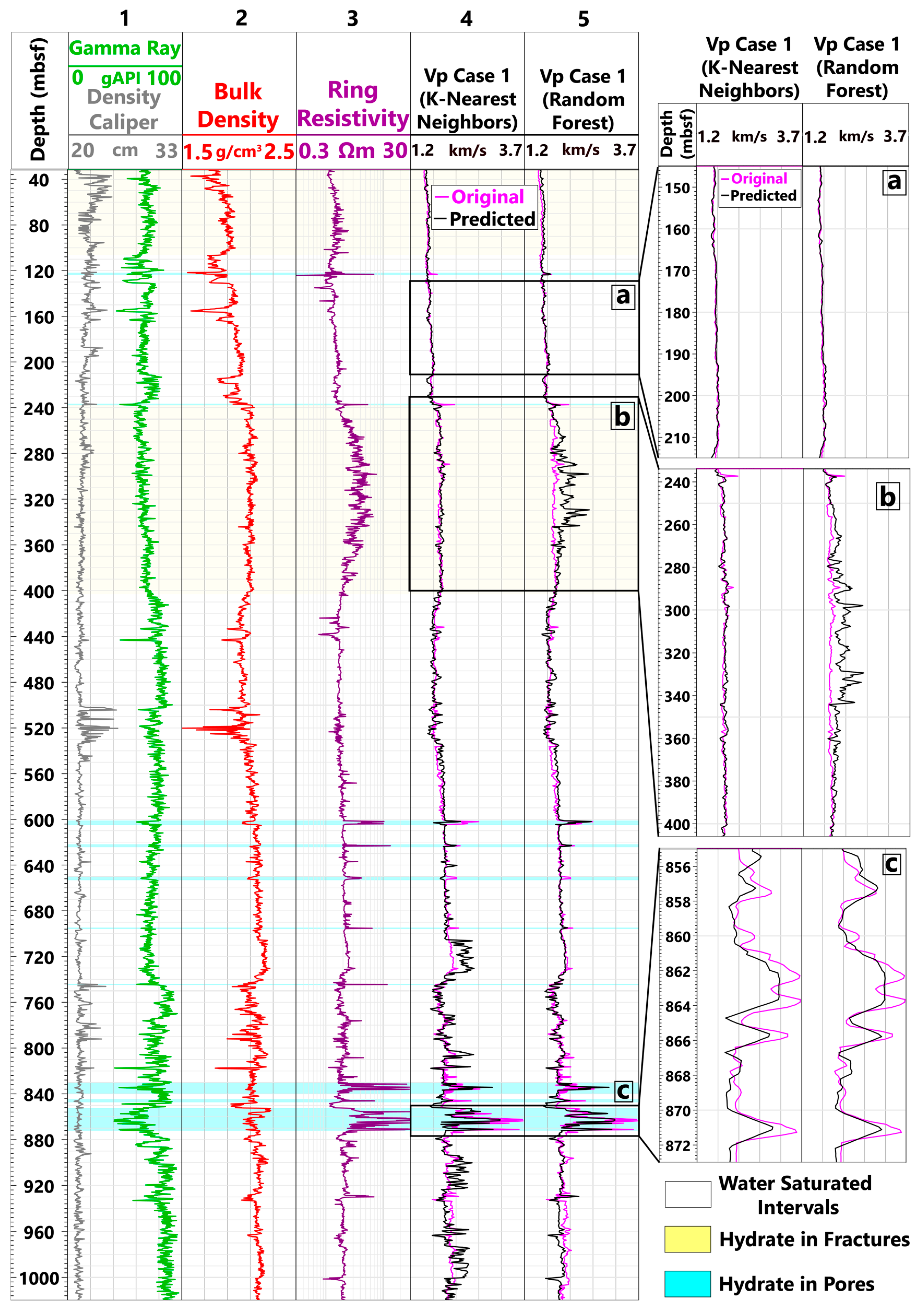
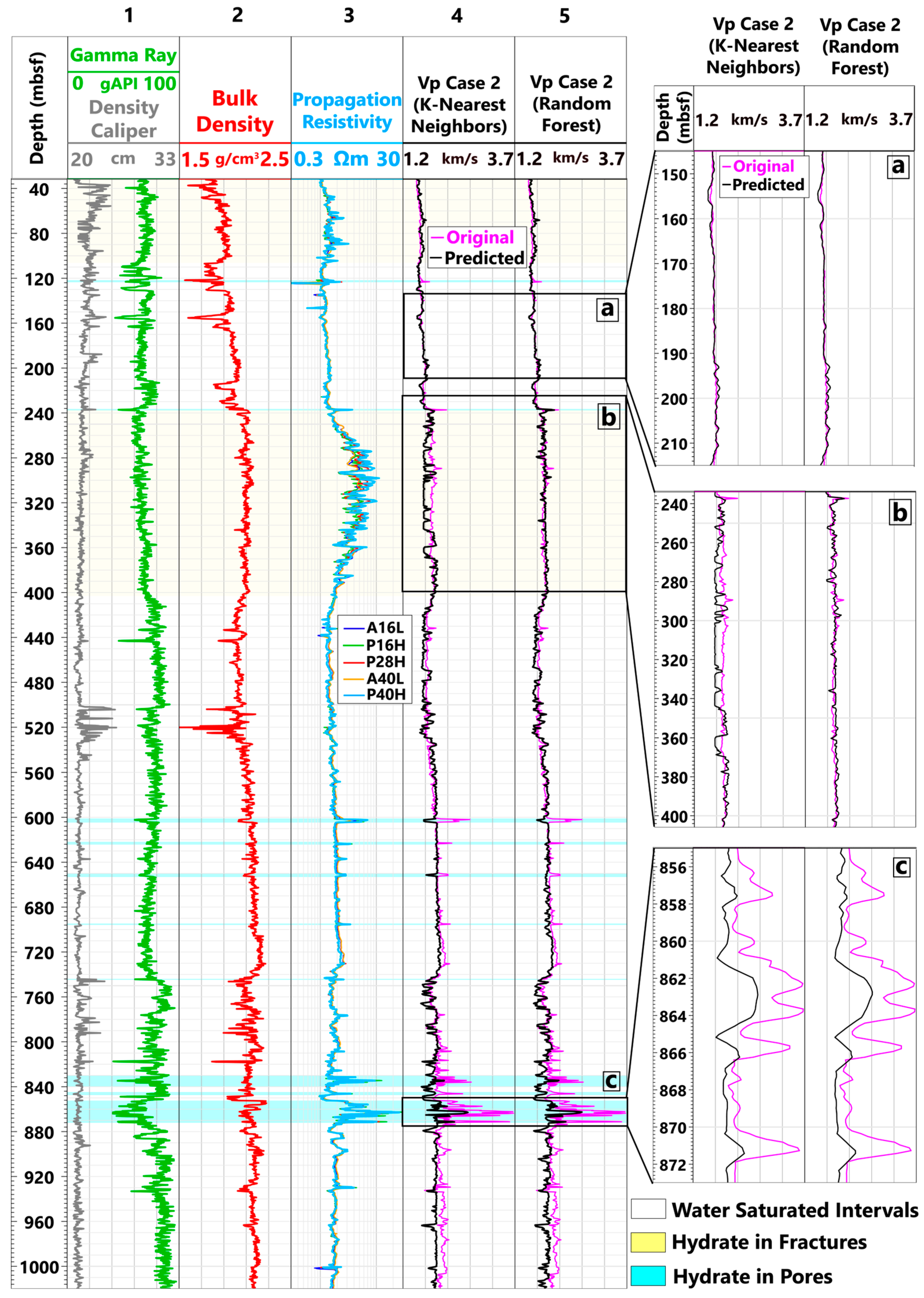
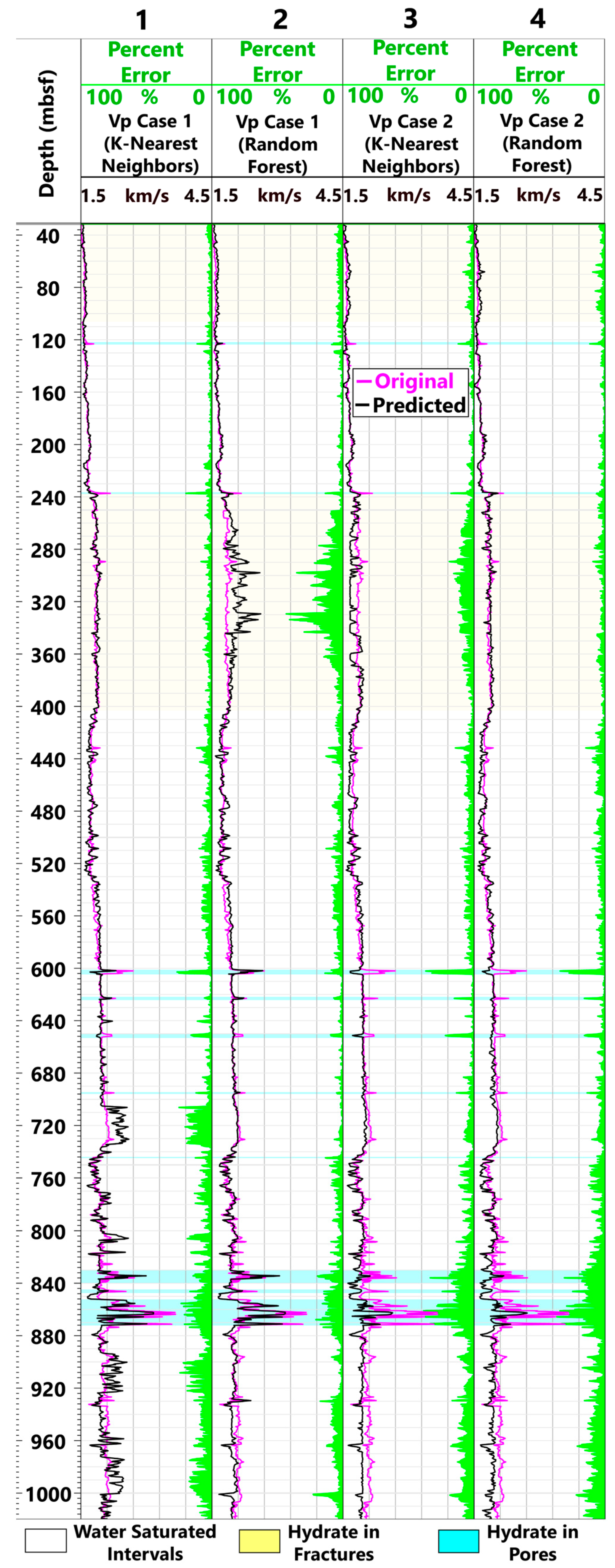
4.1. Formation Vp Prediction
- a.
- Water-Saturated Intervals
- b.
- Hydrate in Fractures
- c.
- Hydrate in Pores
4.2. Bulk Density Prediction
4.3. Prediction at Deeper Depths
4.4. Further Data Limitations
4.5. Neutron Porosity
4.6. Model Application in Non-Hydrate Sites
5. Conclusions
Supplementary Materials
Author Contributions
Funding
Data Availability Statement
Acknowledgments
Conflicts of Interest
Disclaimer
References
- Collett, T.S.; Johnson, A.H.; Knapp, C.C.; Boswell, R. Natural gas hydrates: A review. In AAPG Memoir; American Association of Petroleum Geologists: Tulsa, OK, USA, 2009. [Google Scholar]
- Kvenvolden, K.A.; Lorenson, T.D. The global occurrence of natural gas hydrate. In Geophysical Monograph Series; AGU: Washington, DC, USA, 2001; Volume 124. [Google Scholar] [CrossRef]
- Goldberg, D.; Kleinberg, R.L.; Weinberger, J.L.; Malinverno, A.; McLellan, P.J.; Collett, T.S. Evaluation of Natural Gas-Hydrate Systems Using Borehole Logs. In Geophysical Characterization of Gas Hydrates; Society of Exploration Geophysicists: Houston, TX, USA, 2010; Chapter 16. [Google Scholar] [CrossRef]
- Kerkar, P.B.; Horvat, K.; Mahajan, D.; Jones, K.W. Formation and dissociation of methane hydrates from seawater in consolidated sand: Mimicking methane hydrate dynamics beneath the seafloor. Energies 2013, 6, 6225–6241. [Google Scholar] [CrossRef]
- Li, Z.D.; Tian, X.; Li, Z.; Xu, J.Z.; Zhang, H.X.; Wang, D.J. Experimental study on growth characteristics of pore-scale methane hydrate. Energy Rep. 2020, 6, 933–943. [Google Scholar] [CrossRef]
- Yun, T.S.; Francisca, F.M.; Santamarina, J.C.; Ruppel, C. Compressional and shear wave velocities in uncemented sediment containing gas hydrate. Geophys. Res. Lett. 2005, 32, L10609. [Google Scholar] [CrossRef]
- Oti, E.A.; Cook, A.E.; Phillips, S.C.; Holland, M.E. Using X-ray computed tomography to estimate hydrate saturation in sediment cores from Green Canyon 955, northern Gulf of Mexico. AAPG Bull. 2022, 106, 1127–1142. [Google Scholar] [CrossRef]
- Cook, A.E.; Goldberg, D.S.; Malinverno, A. Natural gas hydrates occupying fractures: A focus on non-vent sites on the Indian continental margin and the northern Gulf of Mexico. Mar. Pet. Geol. 2014, 58, 278–291. [Google Scholar] [CrossRef]
- Collett, T.S.; Ladd, J. Detection of gas hydrate with downhole logs and assessment of gas hydrate concentrations (saturations) and gas volumes on the Blake Ridge with electrical resistivity log data. In Proceedings of the Ocean Drilling Program: Scientific Results; Texas A&M University: College Station, TX, USA, 2000. [Google Scholar] [CrossRef]
- Malinverno, A.; Kastner, M.; Torres, M.E.; Wortmann, U.G. Gas hydrate occurrence from pore water chlorinity and downhole logs in a transect across the northern Cascadia margin (Integrated Ocean Drilling Program Expedition 311). J. Geophys. Res. Solid Earth 2008, 113, B08103. [Google Scholar] [CrossRef]
- Cook, A.E.; Anderson, B.I.; Malinverno, A.; Mrozewski, S.; Goldberg, D.S. Electrical anisotropy due to gas hydrate-filled fractures. Geophysics 2010, 75, F173–F185. [Google Scholar] [CrossRef]
- Helgerud, M.B.; Dvorkin, J.; Nur, A.; Sakai, A.; Collett, T. Elastic-wave velocity in marine sediments with gas hydrates: Effective medium modeling. Geophys. Res. Lett. 1999, 26, 2021–2024. [Google Scholar] [CrossRef]
- Lee, M.W.; Collett, T.S. In-situ gas hydrate hydrate saturation estimated from various well logs at the Mount Elbert Gas Hydrate Stratigraphic Test Well, Alaska North Slope. Mar. Pet. Geol. 2011, 28, 439–449. [Google Scholar] [CrossRef]
- Nelwamondo, F.V.; Golding, D.; Marwala, T. A dynamic programming approach to missing data estimation using neural networks. Inf. Sci. 2013, 237, 49–58. [Google Scholar] [CrossRef]
- Pelckmans, K.; De Brabanter, J.; Suykens, J.A.K.; De Moor, B. Handling missing values in support vector machine classifiers. Neural Netw. 2005, 18, 684–692. [Google Scholar] [CrossRef] [PubMed]
- Han, J.; Kamber, M.; Pei, J. Data Mining: Concepts and Techniques. In Data Mining: Concepts and Techniques; University of Illinois at Urbana-Champaign Micheline Kamber Jian Pei Simon Fraser University: Champaign, IL, USA, 2012. [Google Scholar] [CrossRef]
- Farfour, M.; Mesbah, M. Machine intelligence vs. human intelligence in geological interpretation of seismic data. In Proceedings of the 2020 International Conference on Decision Aid Sciences and Application, DASA 2020, Sakheer, Bahrain, 8–9 November 2020. [Google Scholar] [CrossRef]
- Ismail, A.; Ewida, H.F.; Nazeri, S.; Al-Ibiary, M.G.; Zollo, A. Gas channels and chimneys prediction using artificial neural networks and multi-seismic attributes, offshore West Nile Delta, Egypt. J. Pet. Sci. Eng. 2022, 208, 109349. [Google Scholar] [CrossRef]
- Ramya, J.; Somasundareswari, D.; Vijayalakshmi, P. Gas chimney and hydrocarbon detection using combined BBO and artificial neural network with hybrid seismic attributes. Soft Comput. 2020, 24, 2341–2354. [Google Scholar] [CrossRef]
- Bressan, T.S.; Kehl de Souza, M.; Girelli, T.J.; Junior, F.C. Evaluation of machine learning methods for lithology classification using geophysical data. Comput. Geosci. 2020, 139, 104475. [Google Scholar] [CrossRef]
- Ismail, A.; Radwan, A.A.; Leila, M.; Abdelmaksoud, A.; Ali, M. Unsupervised machine learning and multi-seismic attributes for fault and fracture network interpretation in the Kerry Field, Taranaki Basin, New Zealand. Geomech. Geophys. Geo-Energy Geo-Resour. 2023, 9, 122. [Google Scholar] [CrossRef]
- Hou, M.; Xiao, Y.; Lei, Z.; Yang, Z.; Lou, Y.; Liu, Y. Machine Learning Algorithms for Lithofacies Classification of the Gulong Shale from the Songliao Basin, China. Energies 2023, 16, 2581. [Google Scholar] [CrossRef]
- Lou, Y.; Li, S.; Liu, N.; Liu, R. Seismic volumetric dip estimation via a supervised deep learning model by integrating realistic synthetic data sets. J. Pet. Sci. Eng. 2022, 218, 111021. [Google Scholar] [CrossRef]
- Yang, L.; Sun, S.Z. Seismic horizon tracking using a deep convolutional neural network. J. Pet. Sci. Eng. 2020, 187, 106709. [Google Scholar] [CrossRef]
- Shalaby, M.R.; Jumat, N.; Lai, D.; Malik, O. Integrated TOC prediction and source rock characterization using machine learning, well logs and geochemical analysis: Case study from the Jurassic source rocks in Shams Field, NW Desert, Egypt. J. Pet. Sci. Eng. 2019, 176, 369–380. [Google Scholar] [CrossRef]
- Gjelsvik, E.L.; Fossen, M.; Tøndel, K. Current overview and way forward for the use of machine learning in the field of petroleum gas hydrates. Fuel 2023, 334 Pt 2, 126696. [Google Scholar] [CrossRef]
- Singh, H.; Seol, Y.; Myshakin, E.M. Prediction of gas hydrate saturation using machine learning and optimal set of well-logs. Comput. Geosci. 2021, 25, 267–283. [Google Scholar] [CrossRef]
- Yu, Z.; Tian, H. Application of Machine Learning in Predicting Formation Condition of Multi-Gas Hydrate. Energies 2022, 15, 4719. [Google Scholar] [CrossRef]
- Rebai, N.; Hadjadj, A.; Benmounah, A.; Berrouk, A.S.; Boualleg, S.M. Prediction of natural gas hydrates formation using a combination of thermodynamic and neural network modeling. J. Pet. Sci. Eng. 2019, 182, 106270. [Google Scholar] [CrossRef]
- Graw, J.H.; Wood, W.T.; Phrampus, B.J. Predicting Global Marine Sediment Density Using the Random Forest Regressor Machine Learning Algorithm. J. Geophys. Res. Solid Earth 2021, 126, e2020JB020135. [Google Scholar] [CrossRef]
- Sain, K.; Kumar, P.C. Meta-Attributes and Artificial Networking: A New Tool for Seismic Interpretation; AGU-John Wiley & Sons: Hoboken, NJ, USA, 2022. [Google Scholar] [CrossRef]
- Dumke, I.; Berndt, C. Prediction of seismic p-wave velocity using machine learning. Solid Earth 2019, 10, 1989–2000. [Google Scholar] [CrossRef]
- Flemings, P.B.; Behrmann, J.H.; John, C.M.; the Expedition 308 Scientists. Expedition 308 summary. In Proceedings of the Integrated Ocean Drilling Program; IODP: College Station, TX, USA, 2006; Volume 308. [Google Scholar] [CrossRef]
- Pecher, I.A.; Barnes, P.M.; LeVay, L.J.; the Expedition 372 Scientists. Creeping Gas Hydrate Slides. In Proceedings of the International Ocean Discovery Program, College Station, TX, USA, 26 November 2017–4 January 2018; Volume 372. [Google Scholar] [CrossRef]
- Zoback, M.D. Pore pressure at depth in sedimentary basins. In Reservoir Geomechanics; Cambridge University Press: Cambridge, UK, 2007. [Google Scholar] [CrossRef]
- Liner, C.L. (Ed.) Synthetic Seismogram, Tuning, and Resolution. In Elements of 3D Seismology; Society of Exploration Geophysicists: Houston, TX, USA, 2016; Chapter 19; pp. 213–228. [Google Scholar] [CrossRef]
- Collett, T.S.; Lee, M.W.; Zyrianova, M.V.; Mrozewski, S.A.; Guerin, G.; Cook, A.E.; Goldberg, D.S. Gulf of Mexico Gas Hydrate Joint Industry Project Leg II logging-while-drilling data acquisition and analysis. Mar. Pet. Geol. 2012, 34, 41–61. [Google Scholar] [CrossRef]
- Riedel, M.; Collett, T.S.; Malone, M.J.; Mitchell, M.; Guèrin, G.; Akiba, F.; Blanc-Valleron, M.M.; Ellis, M.; Hashimoto, Y.; Heuer, V.; et al. Gas hydrate drilling transect across northern Cascadia margin–IODP Expedition 311. Geol. Soc. Spec. Publ. 2009, 319, 11–19. [Google Scholar] [CrossRef]
- Collett, T.S.; Boswell, R.; Cochran, J.R.; Kumar, P.; Lall, M.; Mazumdar, A.; Ramana, M.V.; Ramprasad, T.; Riedel, M.; Sain, K.; et al. Geologic implications of gas hydrates in the offshore of India: Results of the National Gas Hydrate Program Expedition 01. Mar. Pet. Geol. 2014, 58, 3–28. [Google Scholar] [CrossRef]
- Kevin Meazell, P.; Flemings, P.B.; Santra, M.; Johnson, J.E. Sedimentology and stratigraphy of a deep-water gas hydrate reservoir in the northern Gulf of Mexico. AAPG Bull. 2020, 104, 1945–1969. [Google Scholar] [CrossRef]
- Santra, M.; Flemings, P.B.; Scott, E.; Kevin Meazell, P. Evolution of gas hydrate-bearing deep-water channel-levee system in abyssal Gulf of Mexico: Levee growth and deformation. AAPG Bull. 2020, 104, 1921–1944. [Google Scholar] [CrossRef]
- Flemings, P.B.; Phillips, S.C.; Boswell, R.; Collett, T.S.; Cook, A.E.; Dong, T.; Frye, M.; Goldberg, D.S.; Guerin, G.; Holland, M.E.; et al. Pressure coring a Gulf of Mexico deep-water turbidite gas hydrate reservoir: Initial results from the University of Texas-Gulf of Mexico 2-1 (UT-GOM2-1) Hydrate Pressure Coring Expedition. AAPG Bull. 2020, 104, 1847–1876. [Google Scholar] [CrossRef]
- Cook, A.E.; Tost, B.C. Geophysical signatures for low porosity can mimic natural gas hydrate: An example from Alaminos Canyon, Gulf of Mexico. J. Geophys. Res. Solid Earth 2014, 119, 7458–7472. [Google Scholar] [CrossRef]
- Frye, M.; Shedd, W.W.; Godfriaux, P.D.; Dufrene, R.S.; Collett, T.S.; Lee, M.W.; Boswell, R.; Jones, E.; McConnell, D.R.; Mrozewski, S.; et al. Gulf of Mexico gas hydrate joint industry project leg II: Results from the Alaminos Canyon 21 Site. In Proceedings of the Annual Offshore Technology Conference, Houston, TX, USA, 3–6 May 2010; Volume 2. [Google Scholar]
- Expedition 311 summary. In Proceedings of the IODP; IODP: College Station, TX, USA, 2006; Volume 311. [CrossRef]
- Rees, E.V.L.; Priest, J.A.; Clayton, C.R.I. The structure of methane gas hydrate bearing sediments from the Krishna-Godavari Basin as seen from Micro-CT scanning. Mar. Pet. Geol. 2011, 28, 1283–1293. [Google Scholar] [CrossRef]
- Frye, M.; Shedd, W.; Boswell, R. Gas hydrate resource potential in the Terrebonne Basin, Northern Gulf of Mexico. Mar. Pet. Geol. 2012, 34, 150–168. [Google Scholar] [CrossRef]
- Hillman, J.I.T.; Cook, A.E.; Daigle, H.; Nole, M.; Malinverno, A.; Meazell, K.; Flemings, P.B. Gas hydrate reservoirs and gas migration mechanisms in the Terrebonne Basin, Gulf of Mexico. Mar. Pet. Geol. 2017, 86, 1357–1373. [Google Scholar] [CrossRef]
- Ellis, D.V.; Singer, J.M. Well Logging for Earth Scientists; Springer: Dordrecht, The Netherlands, 2007. [Google Scholar] [CrossRef]
- Wu, J.; Chen, X.Y.; Zhang, H.; Xiong, L.D.; Lei, H.; Deng, S.H. Hyperparameter optimization for machine learning models based on Bayesian optimization. J. Electron. Sci. Technol. 2019, 17, 26–40. [Google Scholar] [CrossRef]
- Kutty, A.A.; Wakjira, T.G.; Kucukvar, M.; Abdella, G.M.; Onat, N.C. Urban resilience and livability performance of European smart cities: A novel machine learning approach. J. Clean. Prod. 2022, 378, 134203. [Google Scholar] [CrossRef]
- Wakjira, T.G.; Ibrahim, M.; Ebead, U.; Alam, M.S. Explainable machine learning model and reliability analysis for flexural capacity prediction of RC beams strengthened in flexure with FRCM. Eng. Struct. 2022, 255, 113903. [Google Scholar] [CrossRef]
- Su, Y.; Gao, X.; Li, X.; Tao, D. Multivariate multilinear regression. IEEE Trans. Syst. Man Cybern. Part B Cybern. 2012, 42, 1560–1573. [Google Scholar] [CrossRef]
- Ostertagová, E. Modelling using polynomial regression. Procedia Eng. 2012, 48, 500–506. [Google Scholar] [CrossRef]
- Hastie, T.; Tibshirani, R.; Friedman, J. The Elements of Statistical Learning:Data Mining, Inference, and Prediction, 2nd ed.; Springer: New York, NY, USA, 2017; Volume 27, pp. 83–85. [Google Scholar] [CrossRef]
- Wu, X.; Kumar, V.; Ross, Q.J.; Ghosh, J.; Yang, Q.; Motoda, H.; McLachlan, G.J.; Ng, A.; Liu, B.; Yu, P.S.; et al. Top 10 algorithms in data mining. Knowl. Inf. Syst. 2008, 14, 1–37. [Google Scholar] [CrossRef]
- Breiman, L. Random forests. Mach. Learn. 2001, 45, 5–32. [Google Scholar] [CrossRef]
- Biau, G. Analysis of a random forests model. J. Mach. Learn. Res. 2012, 13, 1063–1095. [Google Scholar] [CrossRef]
- Liu, Z.; Liu, J. Seismic-controlled nonlinear extrapolation of well parameters using neural networks. Geophysics 1998, 63, 2035–2041. [Google Scholar] [CrossRef]
- McCormack, M.D. Neural computing in geophysics. Lead. Edge 1991, 10, 11–15. [Google Scholar] [CrossRef]
- McCulloch, W.S.; Pitts, W. A logical calculus of the ideas immanent in nervous activity. Bull. Math. Biophys. 1943, 5, 115–133. [Google Scholar] [CrossRef]
- Nielsen, M.A. Neural Networks and Deep Learning; Determination Press: San Francisco, CA, USA, 2014. [Google Scholar]
- García, S.; Luengo, J.; Herrera, F. Data Preprocessing in Data Mining; Intelligent Systems Reference Library; Springer International Publishing: Cham, Switzerland, 2015; Volume 72. [Google Scholar] [CrossRef]
- Aksoy, S.; Haralick, R.M. Feature normalization and likelihood-based similarity measures for image retrieval. Pattern Recognit. Lett. 2001, 22, 563–582. [Google Scholar] [CrossRef]
- Schlumberger. SonicVISION: Real-Time LWD Sonic for Advanced Drilling Optimization and Formation Evaluation; Schlumberger: Shenzhen, China, 2010. [Google Scholar]
- Schlumberger. EcoScope Log Quality Control Reference Manual; Schlumberger: Shenzhen, China, 2015. [Google Scholar]
- Schlumberger. GeoVISION Brochure: Resistivity Imaging for Productive Drilling; Schlumberger: Shenzhen, China, 2007. [Google Scholar]
- Nguyen, H.; Savary-Sismondin, B.; Patacz, V.; Jenssen, A.; Kifle, R.; Bertrand, A. Application of random forest algorithm to predict lithofacies from well and seismic data in Balder field, Norwegian North Sea. AAPG Bull. 2022, 106, 2239–2257. [Google Scholar] [CrossRef]
- Zou, C.; Zhao, L.; Xu, M.; Chen, Y.; Geng, J. Porosity Prediction With Uncertainty Quantification From Multiple Seismic Attributes Using Random Forest. J. Geophys. Res. Solid Earth 2021, 126, e2021JB021826. [Google Scholar] [CrossRef]
- Lorenzen, R. Multivariate linear regression of sonic logs on petrophysical logs for detailed reservoir characterization in producing fields. Interpretation 2018, 6, T543–T553. [Google Scholar] [CrossRef]
- Guerin, G.; Goldberg, D. Sonic waveform attenuation in gas hydrate-bearing sediments from the Mallik 2L-38 research well, Mackenzie Delta, Canada. J. Geophys. Res. 2002, 107, EPM-1. [Google Scholar] [CrossRef]
- Tobin, H.; Hirose, T.; Ikari, M.; Kanagawa, K.; Kimura, G.; Kinoshita, M.; Kitajima, H.; Saffer, D.; Yamaguchi, A.; Eguchi, N.; et al. Expedition 358 summary. In Proceedings of the Integrated Ocean Drilling Program; IODP: College Station, TX, USA, 2020. [Google Scholar] [CrossRef]
- Saffer, D.M.; Wallace, L.M.; Barnes, P.M.; Pecher, I.A.; Petronotis, K.E.; LeVay, L.J.; Bell, R.E.; Crundwell, M.P.; Engelmann de Oliveira, C.H.; Fagereng, A.; et al. Expedition 372B/375 summary. In Proceedings of the Integrated Ocean Drilling Program; IODP: College Station, TX, USA, 2019. [Google Scholar] [CrossRef]
- Almenningen, S.; Iden, E.; Fernø, M.A.; Ersland, G. Salinity Effects on Pore-Scale Methane Gas Hydrate Dissociation. J. Geophys. Res. Solid Earth 2018, 123, 5599–5608. [Google Scholar] [CrossRef]
- Hanor, J.S.; Mercer, J.A. Spatial variations in the salinity of pore waters in northern deep water Gulf of Mexico sediments: Implications for pathways and mechanisms of solute transport. Geofluids 2010, 10, 83–93. [Google Scholar] [CrossRef]


| Hole | Location | Drilling Project | Water Depth (m) | Total Depth Drilled (mbsf) | Water Saturated Intervals (m) | Hydrate in Fractures (m) | Hydrate in Pores (m) |
|---|---|---|---|---|---|---|---|
| GC955-H | Gulf of Mexico | JIP Leg II | 2033 | 590 | 412 | 144 | 34 |
| GC955-I | 2064 | 671 | 666 | 0 | ~5 | ||
| GC955-Q | 1985 | 461 | 437 | 0 | ~24 | ||
| AC21-A | 1490 | 536 | 436 | 79 | 21 | ||
| AC21-B | 1488 | 340 | 301 | 0 | 39 | ||
| WR313-G | 2000 | 1043 | <753 | >246 | 44 | ||
| WR313-H | 1966 | 1000 | 626 | 325 | 49 | ||
| U1325A | Cascadia Margin | IODP Expedition 311 | 2192 | 350 | >349 | 0 | <0.23 |
| U1327A | 1305 | 300 | 282 | 0 | 18 | ||
| U1328A | 1267 | 300 | 254 | 46 | 0 | ||
| NGHP-01-02A | Bay of Bengal | NGHP Expedition 01 | 1058 | 50 | 50 | 0 | 0 |
| NGHP-01-02B | 1058 | 250 | 250 | 0 | 0 | ||
| NGHP-01-03A | 1076 | 300 | 91 | 209 | 0 | ||
| NGHP-01-04A | 1081 | 300 | 280 | 20 | 0 | ||
| NGHP-01-05A | 945 | 200 | 161 | 39 | 0 | ||
| NGHP-01-05B | 945 | 200 | 163 | 37 | 0 | ||
| NGHP-01-06A | 1160 | 350 | 339 | 11 | 0 | ||
| NGHP-01-07A | 1285 | 260 | 220 | 40 | 0 | ||
| NGHP-01-10A | 1038 | 205 | 82 | 123 | 0 | ||
| NGHP-01-11A | 1007 | 200 | 180 | 20 | 0 | ||
| NGHP-01-08A | 1689 | 350 | 313 | 37 | 0 | ||
| NGHP-01-09A | 1935 | 330 | 230 | 100 | 0 |
| Holes | Location | Gas Hydrate Occurrence | LWD Tools | Logs Used |
|---|---|---|---|---|
| GC955-H GC955-I GC955-Q AC21-A AC21-B | Gulf of Mexico | Gas hydrate occurs in all the holes. | EcoScope geoVISION sonicVISION | Density Caliper (DCAV), Bulk Density (RHOB), Calibrated and Filtered Gamma Ray (GRMA_FILT), RING Resistivity, Propagation Resistivity (A16L, A40L, P16H, P28H, P40H), Vp |
| U1327A U1328A U1325A | Cascadia Margin | Gas hydrate occurs in holes U1327A and U1328A. | adnVISION EcoScope geoVISION sonicVISION | Density Caliper (DCAV), Bulk Density (RHOB), Calibrated and Filtered Gamma Ray (GRMA_FILT), RING Resistivity, Propagation Resistivity (A16L, A40L, P16H, P28H, P40H), Vp |
| NGHP-01-02A NGHP-01-02B NGHP-01-03A NGHP-01-04A NGHP-01-05A NGHP-01-05B NGHP-01-06A NGHP-01-07A NGHP-01-08A NGHP-01-09A NGHP-01-10A NGHP-01-11A | Bay of Bengal | Gas hydrate occurs in all the holes except 02A and 02B | EcoScope geoVISION sonicVISION | Density Caliper (DCAV), Bulk Density (RHOB), Calibrated and Filtered Gamma Ray (GRMA_FILT), RING Resistivity, Propagation Resistivity (A16L, A40L, P16H, P28H, P40H), Vp |
| Multilinear Regression | ||||||
| Training R2 (%) | Training MAPE (%) | Validation R2(%) | Validation MAPE (%) | Test R2 (%) | Test MAPE (%) | |
| Vp Case 1 | 56 | 4.18 | 55 | 4.18 | 59 | 5.69 |
| Vp Case 2 | 62 | 3.60 | 64 | 3.46 | 53 | 6.45 |
| ρb Case 1 | 31 | 5.18 | 31 | 5.12 | 49 | 5.17 |
| ρb Case 2 | 46 | 4.13 | 48 | 4.13 | 41 | 3.14 |
| Polynomial Regression (4th Order) | ||||||
| Training R2 (%) | Training MAPE (%) | Validation R2(%) | Validation MAPE (%) | Test R2 (%) | Test MAPE (%) | |
| Vp Case 1 | 91 | 2.46 | 90 | 2.48 | 50 | 3.79 |
| Vp Case 2 | 88 | 2.02 | 0.015 | 4.83 | 7.0 | 71.4 |
| ρb Case 1 | 62 | 3.54 | 60 | 3.49 | 33 | 160 |
| ρb Case 2 | 82 | 2.33 | 0 | 11 | 0 | 155 |
| Polynomial Regression (4th Order) with Ridge Regularization | ||||||
| Training R2 (%) | Training MAPE (%) | Validation R2(%) | Validation MAPE (%) | Test R2 (%) | Test MAPE (%) | |
| Vp Case 1 | 85 | 2.69 | 83 | 2.7 | 74 | 2.99 |
| Vp Case 2 | 82 | 2.42 | 81 | 2.34 | 55 | 4.99 |
| ρb Case 1 | 57 | 3.86 | 57 | 3.8 | 42 | 5.16 |
| ρb Case 2 | 75 | 2.78 | 75 | 2.81 | 25 | 2.70 |
| K Nearest Neighbors | ||||||
| Training R2 (%) | Training MAPE (%) | Validation R2(%) | Validation MAPE (%) | Test R2 (%) | Test MAPE (%) | |
| Vp Case 1 | 100 | 0 | 94 | 1.98 | 73 | 3.45 |
| Vp Case 2 | 100 | 0 | 86 | 1.79 | 64 | 4.4 |
| ρb Case 1 | 100 | 0 | 76 | 2.55 | 75 | 2.00 |
| ρb Case 2 | 100 | 0 | 85 | 1.86 | 66 | 2.65 |
| Random Forest | ||||||
| Training R2 (%) | Training MAPE (%) | Validation R2(%) | Validation MAPE (%) | Test R2 (%) | Test MAPE (%) | |
| Vp Case 1 | 99 | 1.07 | 96 | 1.60 | 70 | 3.96 |
| Vp Case 2 | 97 | 1.05 | 91 | 1.60 | 63 | 4.40 |
| ρb Case 1 | 93 | 1.51 | 81 | 2.30 | 72 | 2.19 |
| ρb Case 2 | 95 | 1.16 | 89 | 1.71 | 49 | 3.18 |
| Multilayer Perceptron | ||||||
| Training R2 (%) | Training MAPE (%) | Validation R2(%) | Validation MAPE (%) | Test R2 (%) | Test MAPE (%) | |
| Vp Case 1 | 56 | 4.20 | 55 | 4.19 | 59 | 5.66 |
| Vp Case 2 | 62 | 3.59 | 63 | 3.45 | 52 | 6.53 |
| ρb Case 1 | 46 | 4.47 | 45 | 4.40 | 57 | 2.70 |
| ρb Case 2 | 0 | 6.37 | 0 | 6.38 | 0.1 | 11 |
| Random Forest | K Nearest Neighbors | ||||
|---|---|---|---|---|---|
| R2 | MAPE | R2 | MAPE | ||
| Vp Case 1 (Input Logs: Gamma Ray, Bulk Density, Ring Resistivity) | Complete Log Interval | 70% | 3.9% | 73% | 3.4% |
| Water-Saturated | 74% | 3.0% | 75% | 3.6% | |
| Hydrate in Fractures | 54% | 5.9% | 73% | 2.4% | |
| Hydrate in Pores | 81% | 6.5% | 71% | 10% | |
| Vp Case 2 (Input Logs: Gamma Ray, Bulk Density, Propagation Resistivity) | Complete Log Interval | 63% | 4.4% | 64% | 4.4% |
| Water-Saturated | 66% | 4.7% | 70% | 4.0% | |
| Hydrate in Fractures | 68% | 2.8% | 48% | 4.2% | |
| Hydrate in Pores | 69% | 14% | 63% | 15% | |
| ρb Case 1 | Complete Log Interval | 72% | 2.2% | 75% | 2.0% |
Disclaimer/Publisher’s Note: The statements, opinions and data contained in all publications are solely those of the individual author(s) and contributor(s) and not of MDPI and/or the editor(s). MDPI and/or the editor(s) disclaim responsibility for any injury to people or property resulting from any ideas, methods, instructions or products referred to in the content. |
© 2023 by the authors. Licensee MDPI, Basel, Switzerland. This article is an open access article distributed under the terms and conditions of the Creative Commons Attribution (CC BY) license (https://creativecommons.org/licenses/by/4.0/).
Share and Cite
Naim, F.; Cook, A.E.; Moortgat, J. Estimating Compressional Velocity and Bulk Density Logs in Marine Gas Hydrates Using Machine Learning. Energies 2023, 16, 7709. https://doi.org/10.3390/en16237709
Naim F, Cook AE, Moortgat J. Estimating Compressional Velocity and Bulk Density Logs in Marine Gas Hydrates Using Machine Learning. Energies. 2023; 16(23):7709. https://doi.org/10.3390/en16237709
Chicago/Turabian StyleNaim, Fawz, Ann E. Cook, and Joachim Moortgat. 2023. "Estimating Compressional Velocity and Bulk Density Logs in Marine Gas Hydrates Using Machine Learning" Energies 16, no. 23: 7709. https://doi.org/10.3390/en16237709
APA StyleNaim, F., Cook, A. E., & Moortgat, J. (2023). Estimating Compressional Velocity and Bulk Density Logs in Marine Gas Hydrates Using Machine Learning. Energies, 16(23), 7709. https://doi.org/10.3390/en16237709