Probabilistic Wind Speed Forecasting for Wind Turbine Allocation in the Power Grid

Abstract

To face the growing electricity demand, several countries have adopted the solution of clean energy and use renewable energy sources (e.g., wind and solar) to reinforce the stability of the power network, especially during peak demand periods. Forecasting wind power generation is one of the important tasks for the network regulator. This paper deals with the probabilistic forecasting of hourly wind speed time series. In this approach, instead of evaluating a single-point forecast, an intraday interval prediction is provided, which allows modeling the probability distribution of the wind speed process at any specific hour. Practically, the quantification of uncertainty might be of particular interest for risk management purposes associated with wind power generation. The definition of interval prediction is based on the notion of conditional quantiles. In this paper, we introduce a new statistical approach, which deals with the nonstationarity behavior of the wind speed process, to define the conditional quantile predictor. The proposed approach was applied and evaluated on hourly wind speed processes. The suggested methodology provides accurate single-point forecasts using the conditional median as the predictor. Furthermore, the obtained hourly interval predictions are small and well adapted to the shape of the daily wind speed curves, which confirms the efficiency of the proposed approach.

1. Introduction

Arid regions, such as the Arabian Peninsula countries, are characterized by hot and humid summers in which the temperature and relative humidity can reach 46 °C and 100%, respectively. In these regions, rainfall is very scarce. For instance, the mean annual total rainfall in Abu Dhabi in the United Arab Emirates (UAE) is 63 mm/y and the mean number of rainy days is 11 d/y. Despite the harsh weather conditions, substantial socio-economic growth is being observed in the region with a rapid increase in the population and urbanization rate, as well as significant industrialization growth and expansion of the agricultural sector. This growth is associated with a soar in energy demand mostly to meet air-conditioning and desalination needs (e.g., in Abu Dhabi, 95% of potable water is obtained through desalination). Demand for electricity is rising; it has nearly doubled during the last decade and will continue to grow by seven to eight percent annually for several years to come. For instance, in Abu Dhabi, the consumption peak in August 2009 was at 6.255 MW compared to 5.616 MW in 2008. This peak power demand is expected to rise to 11.2 MW by 2015 and 15.5 MW by 2020 (see [1]). Although most of the growth is fueled by hydrocarbon resources, these countries are seriously exploring the deployment and integration of renewable energy sources in their future energy mix.

The generation of electricity is by far the largest single producer of CO₂ emissions in the region and was responsible for an average of 40% of the region’s total CO₂ emissions in 2009, surpassing even 50% in some countries. Therefore, the use of renewable energy sources, such as solar and wind, come as an interesting solution to face the increase in electricity demand.

Wind resources are considered as one of the reliable sources of energy generation in the region. The accurate forecast of wind speed is a challenging task. The high variability in wind power production is mainly explained by the large volatility in wind speed caused by the dynamic nature of the atmosphere. Wind power forecasts might be obtained either through statistical modeling of the wind speed time series and, then, transformation of the forecasts through a power curve (see, for instance, [2] for more details) or using physical models based on numerical weather forecasts (see, e.g., [3]).

Several statistical approaches have been proposed in the literature for wind speed forecasting, for instance machine learning models such as artificial neural networks (see [4] and the bibliography therein) and support vector machine methods [5]. Autoregressive models were used by [6,7,8], whereas Markov chains were introduced by [9,10], among others. One can notice that most of the papers in the literature discussed the single-point forecasts of wind speed, while the need to quantify wind speed forecast uncertainty and communicate the associated risk required more focus on probabilistic forecasts. In the short-term context, probabilistic forecasts might be more relevant than single-point forecasts for the planner to build wind-power-generation scenarios and to help in the management and control of the smart electrical network (see [11,12,13]).

Functional data analysis is a new statistical field that has received an increasing interest in the last few years. Its main purpose is to provide tools for describing and modeling sets of curves. Reference [14] provides an interesting description of the available procedures dealing with functional observations, whereas [15] presents a completely nonparametric point of view of functional data analysis. These functional approaches mainly generalize multivariate statistical procedures to data taking values in some functional spaces and have been proven to be useful in a number of domains including load forecasting [16]. Functional time series analysis is more appropriate than longitudinal data models or time series analysis when repeated measurements are observed for each curve (see [17] for more details).

The focus of the present paper is on the estimation of predictive intervals for hourly wind speed measures at four sites in the U.A.E. More precisely, the target is not to forecast the value of hourly wind speed but also estimate an interval with the coverage probability $\alpha \in (0,1)$ of the observed measure of wind speed. Such interval can be obtained by estimating the lower band (respectively upper band), which corresponds to the $(1-\alpha )/2$-th (respectively $(1+\alpha )/2$-th) conditional quantile. Conditional interval prediction when the covariate is a vector has been introduced in the statistical literature by several authors (see, for instance, [18,19]). This paper aimed to generalize the notion of the conditional predictive interval when the covariate is a curve (see [20]). Therefore, a nonparametric estimator of the conditional quantiles is introduced when the covariate takes values in an infinite-dimensional space. The proposed nonparametric approach is a flexible tool that does not require any specification of the form of the model or assume a certain probabilistic model for the data. Many statistical problems are treated with nonparametric estimation techniques (see, for instance, [21,22]. This paper is organized as follows. Section 2 introduces the notion of functional time series and shows how we can switch from a classical time series to a functional one. Section 2.2 outlines the notations and the form of the kernel-smoothed estimator of conditional quantiles when the covariate is a curve. In Section 2.3, we extend the use of this estimator to build conditional interval predictions in the time series framework and, then, improve it by using a clustering-discrimination procedure, which allows mimicking the stationarity assumption. A comparison of the results obtained by the proposed methods, based on wind speed data, is detailed in Section 3. A discussion of the results is provided in Section 4.

2. Materials and Methods

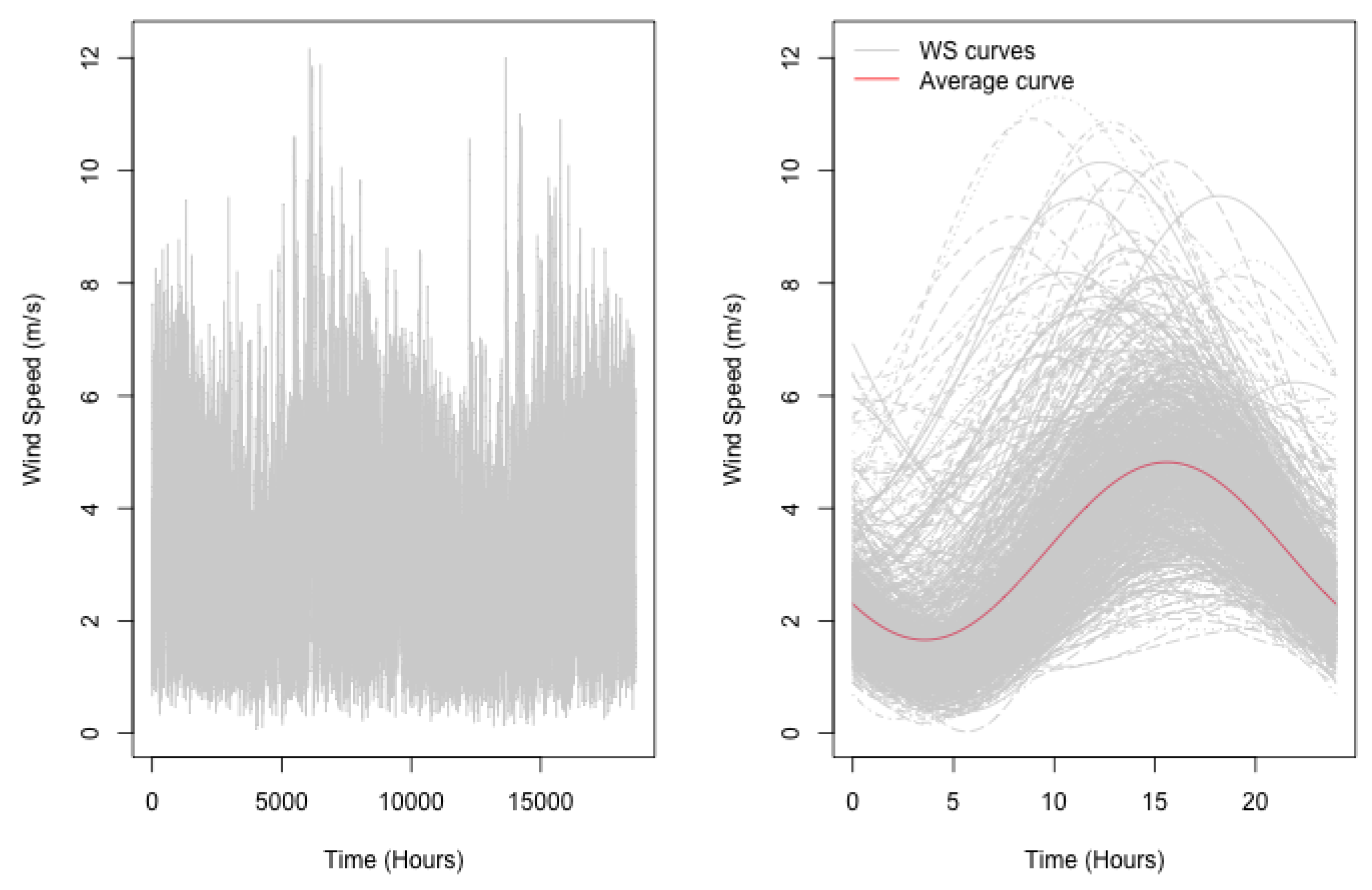
2.1. The Functional Time Series Concept

In this section, we show how the functional data concept can be adapted to wind speed time series analysis. To make the introduction of this concept easier, let us proceed by an example. The dataset analyzed in this paper contains hourly observations of a stochastic process $\xi \left(t\right)$, $t\in {\mathbb{R}}^{+}$. Here, $\xi \left(t\right)$ represents the wind speed measured in meters per second (m/s) at time t (hour in this specific case) at any wind station. This process has been observed, for instance, in Madinat Zayed station, at each hour from 16 July 2008 to 31 August 2010 (which corresponds to a total of 777 days). The shape of the hourly wind speed time series is plotted in the left panel of Figure 1. Since we are interested in the intraday wind speed time series prediction, we divided the observed original time series $\left(\xi \right(t\left)\right)$ of hourly wind speed measures into $n=777$ segments ${\left(X_i\left(t\right)\right)}_{i=1,\dots ,n}$ of length 24, which corresponds to a functional observation. Formally, let $[0,T]$ be the time interval on which the process $\xi \left(t\right)$ is observed. We divided this interval into subintervals of length 24, say $[\ell \times 24,(\ell +1)\times 24]$, $\ell =0,1,\dots ,n-1$ with $n=T/24$. We denote $X_i\left(t\right)$ as the functional-valued discrete-time stochastic process defined, for any $i=1,\dots ,n$ and $\forall t\in [0,24)$, by $X_i:=X_i\left(t\right)=\xi (t+24(i-1))$.

The right panel of Figure 1 shows the corresponding daily wind speed curves ${\left(X_i\left(t\right)\right)}_{i=1,\dots ,n}$ observed at Madinat Zayed station, which were deduced from the original process $\xi \left(t\right)$.

In the following section, we define the general setting of quantile regression when the covariate takes values in some infinite-dimensional space and the observations are supposed to be dependent. Then, we provide a kernel-type estimator of them.

2.2. Quantile Regression Model When the Covariate Is a Function

2.2.1. Definition of the $\alpha$-th Conditional Quantile

Let $(X,Y)$ be $\mathcal{E}\times \mathbb{R}$-valued random elements, where $\mathcal{E}$ is some semimetric abstract space. Denote by $d(·,·)$ a semimetric associated with the space $\mathcal{E}$. Suppose now that we observe a sequence ${(X_i,Y_i)}_{i=1,\cdots ,n}$ of copies of $(X,Y)$, which we assume to be stationary and dependent.

Let $F(·\mid x)$ be the conditional probability distribution function of Y given $X=x$ defined as:

$$\begin{array}{c}\hfill \forall y\in \mathbb{R},F(y\mid x)=\mathbb{P}(Y\le y\mid X=x).\end{array}$$

The conditional quantile, of order $\alpha$ in $(0,1)$, is given by:

$$\begin{array}{c}\hfill Q_{\alpha }\left(x\right)=inf\{y:F(y\mid x)\ge \alpha \}.\end{array}$$

(1)

If in addition, we suppose, for any fixed $x\in \mathcal{E}$, that $F(·\mid x)$ is a continuously differentiable real function, then F admits a unique conditional quantile. Therefore, for any $\alpha \in (0,1)$, $Q_{\alpha }\left(x\right)$ satisfies:

$$\begin{array}{c}\hfill F(Q_{\alpha }\left(x\right)\mid x)=\alpha .\end{array}$$

2.2.2. Nadaraya–Watson-Type Estimator of $Q_{\alpha }\left(x\right)$

It is clear that an estimator of $Q_{\alpha }\left(x\right)$ can easily be deduced from an estimator of $F(y\mid x)$.

A kernel-smoothed-type (KS) estimator, say $F_n^{KS}(y\mid x)$, of the conditional cumulative distribution function $F(y\mid x)$ is given by:

$$\begin{array}{c}\hfill F_n^{KS}(y\mid x)=\sum _{i=1}^n\mathcal{W}(x,X_i)H\left(\frac{y-Y_i}{h_n}\right),\end{array}$$

(2)

where $\mathcal{W}(x,X_i)$ are the Nadaraya–Watson weights defined, for $i=1,\dots ,n$, as:

$$\mathcal{W}(x,X_i)=\frac{K\left(\frac{d(x,X_i)}{h_n}\right)}{{\sum }_{i=1}^{n}K\left(\frac{d(x,X_i)}{h_n}\right)},$$

where $K:[0,\infty )\to [0,\infty )$ is a real-valued probability density function, called the kernel and chosen by the user. The function $H(·)$ is a given smoothed cumulative distribution function, and $h_n$, called the bandwidth, is a sequence of positive real numbers, which goes to zero as n goes to infinity.

Whereas the Euclidean norm is a standard distance measure in finite-dimensional spaces, the notion of the semi-norm or semimetric arises in this infinite-dimensional functional space setup. Several options for the semimetric $d(·,·)$ are available in the statistical literature (see [15] for an overview). The semimetric $d(·,·)$ plays a key role related to the so-called “curse of dimensionality” in nonparametric functional estimation. In practice the “curse of dimensionality” is described as the sparseness of data in the observation region when the data space dimension grows. This problem is especially dramatic in the infinite-dimensional context of functional data. Reference [15] discussed semimetric choices in functional data context that allow to achieve a convergence rate in nonparametric estimation similar to the one obtained in the finite-dimensional case. It is worth noting that, in order to overcome the “curse of dimensionality”, one uses a semimetric instead of a metric. Moreover, It has been proven in the nonparametric statistics literature that the choice of the kernel K does not significantly affect the quality of the estimator. However, the determinant tuning parameters for a good asymptotic and practical behavior of the estimator given by Equation (2) are the bandwidth and the semimetric.

From Equation (1), one can deduce that a natural kernel-smoothed-type estimator, say $Q_{\alpha ,n}^{KS}\left(x\right)$, of the $\alpha$-th conditional quantile $Q_{\alpha }\left(x\right)$ is given, for a fixed $x\in \mathcal{E}$, by:

$$\begin{array}{c}\hfill Q_{\alpha ,n}^{KS}\left(x\right)=inf\{y:F_n^{KS}(y\mid x)\ge \alpha \},\end{array}$$

(3)

which satisfies:

$$\begin{array}{c}\hfill F_n^{KS}(Q_{\alpha ,n}^{KS}\left(x\right)\mid x)=\alpha .\end{array}$$

In the next section, it is indicated how this general setting of conditional quantiles can be applied to time series forecasting and interval prediction.

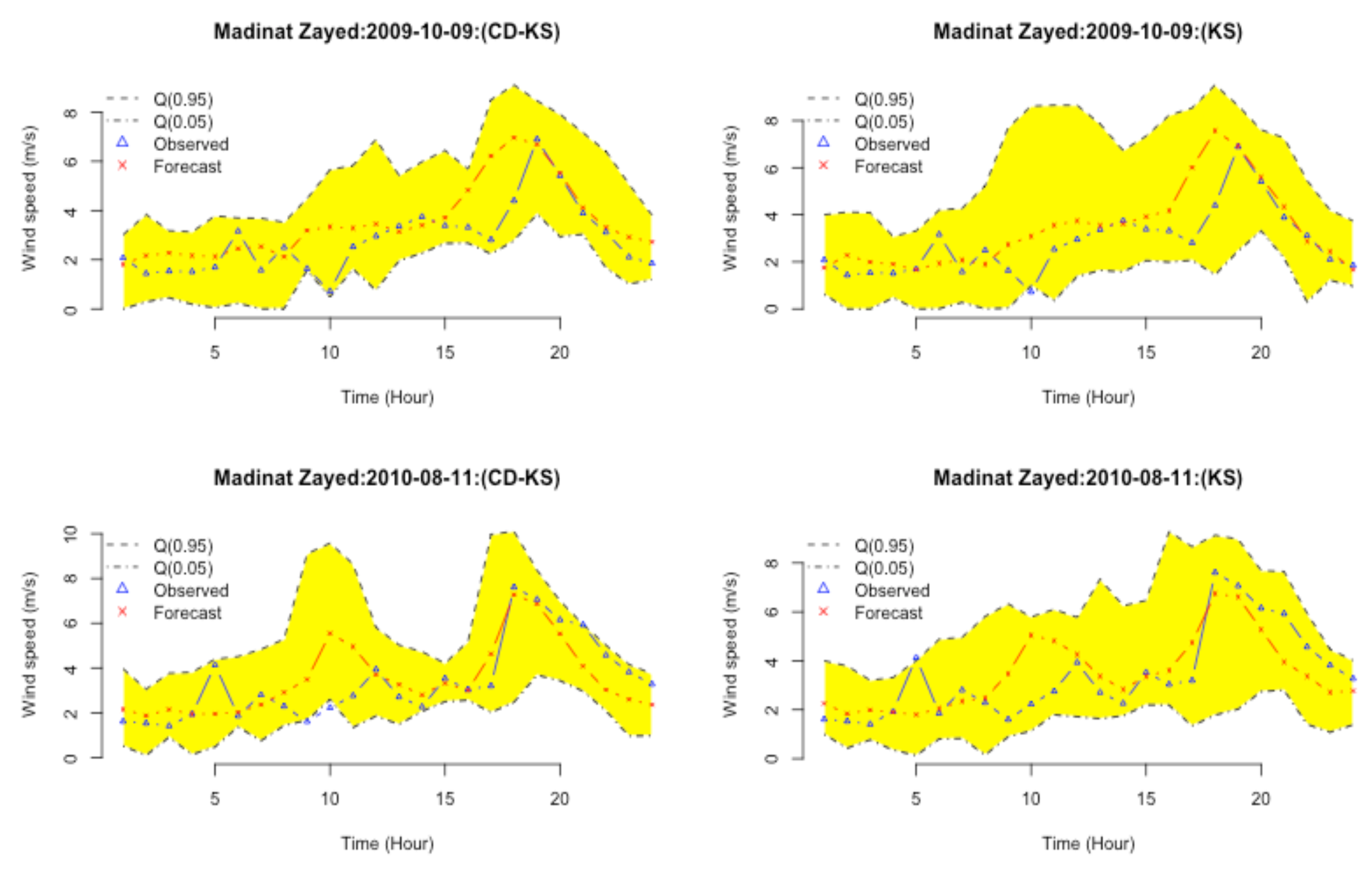
2.3. Interval Prediction for Nonstationary Processes

In nonlinear time series analysis, authors are usually interested in single-point prediction by using as predictor statistics, such as the regression function, the mode regression or the median regression. All these statistics summarize the distribution of the concerned random variable (wind speed in our case). In practice, usually, further information about the distribution might be of interest. Predictive intervals are considered as a common way to summarize forecast accuracy, and they are often more informative than a single-point prediction.

Let ${\left(\xi \left(t\right)\right)}_{t\in [0,T]}$ be the continuous-time wind speed process observed over a time interval $[0,T]$. In this paper, we consider that, for a fixed horizon prediction $r\ge 0$, the process ${\xi \left(t\right)}_{t\in \mathbb{R}}$ satisfies the Markov property, which means that the probability distribution of the future value of the wind process given the whole past depends only on the process values at the last day. This property can be written formally as follows:

$$\xi (T+r){\mid }_{\left\{\xi \right(t),t\in [0,T\left)\right\}}\stackrel{\mathcal{D}}{=}\xi (T+r){\mid }_{\left\{\xi \right(t),t\in [T-24,T\left)\right\}},$$

where $\mathcal{D}$ denotes a probability distribution.

For a fixed horizon r and a given probability $\alpha \in (0,1)$, our target is to build, at time $T+r$, a conditional predictive interval, say ${\Xi }_{\alpha }\left(r\right)\equiv {\Xi }_{\alpha }(r,X=X_n)\subset \mathbb{R}$, for the random variable $Y_r:=\xi (T+r)$. Here, $X_n$ is the last daily wind speed curve and defined as $X_n:=\{\xi \left(t\right),T-24<t<T\}$. The $\alpha$-th predictive interval (PI) ${\Xi }_{\alpha }\left(r\right)$ is such an interval with the coverage probability $\alpha \in (0,1)$, i.e.,

$$\mathbb{P}\left(Y_r\in {\Xi }_{\alpha }\left(r\right)\mid X=X_n\right)=\alpha .$$

In this paper, the construction of the conditional PI is based on the $\alpha$-th conditional quantile. Therefore, for any fixed $X_n$ and $\alpha \in (0,1)$, it takes the following form:

$${\Xi }_{\alpha }\left(r\right):=\left[Q_{0.5-\alpha /2,r}\left(X_n\right),Q_{0.5+\alpha /2,r}\left(X_n\right)\right],$$

where $Q_{\alpha ,r}\left(X_n\right)$ is the $\alpha$-th quantile of $Y_r$ given $X=X_n$.

For a fixed horizon r and given a sample ${(X_i,Y_{i,r})}_{i=1,\dots ,n}$, where n is the number of days in the original time series of length T where

$$X_i:=\{\xi \left(t\right),(i-1)\times 24<t<i\times 24\}$$

and

$$Y_{i,r}=\xi (i\times 24+r),$$

then, following Equation (3), the $\alpha$-th conditional quantile of the wind speed $Y_r$ at time $T+r$, given the last wind speed daily curve $X_n$ is defined as:

$$\begin{array}{c}\hfill Q_{\alpha ,n,r}^{KS}\left(X_n\right)=inf\{y:F_{n,r}^{KS}(y\mid X_n)\ge \alpha \},\end{array}$$

(4)

where

$$F_{n,r}^{KS}\left(y\right|X_n)=\sum _{i=1}^{n-1}\mathcal{W}(X_n,X_i)H\left(\frac{y-Y_{i,r}}{h_n}\right),$$

Finally, a kernel-smoothed estimation of the PI at a horizon r, named ${\Xi }_{\alpha ,n}^{KS}\left(r\right)$ is defined as:

$${\Xi }_{\alpha ,n}^{KS}\left(r\right):=\left[Q_{0.5-\alpha /2,n,r}^{KS}\left(X_n\right),Q_{0.5+\alpha /2,n,r}^{KS}\left(X_n\right)\right].$$

Clustering-Discrimination Kernel-Smoothed Approach (CD-KS)

In this subsection, we provide a new approach to estimate conditional quantiles and, thereafter, build prediction intervals that deal with the nonstationarity issue of the wind speed process $\xi \left(t\right)$. The proposed prediction procedure consists of the following main steps: (a) classification of the sample of n historical daily wind speed curves into M clusters containing typical daily wind speed curves. For this step, we used an unsupervised classification method since we do not have any “a priori” knowledge about susceptible common patterns. (b) Assign to the last observed daily wind speed curve $X_n$ the most-“appropriate” cluster. This step aims to identify days containing similar information as the last observed day. In other words, we look at the historical daily wind speed curves for those that describe a similar behavior to the one we observe today. (c) Apply the KS estimator given by (4) to obtain the $\alpha$-th conditional quantile of $Y_{n+1,r}$ given $X_n$. The following algorithm describes in more detail the CD-KS prediction approach:

Step 1: 

unsupervised curve classification.

Suppose that we have $(n-1)$ historical daily wind speed curves $X_1,\dots ,X_{n-1}$. In this step, we automatically split these $(n-1)$ curves into M clusters, say ${\mathcal{G}}_1,{\mathcal{G}}_2,\dots ,{\mathcal{G}}_M$. Because we do not have at hand any categorical response variable and the dataset is clearly of a functional nature, then this problem can be seen as an unsupervised curve classification. Several statistical approaches have been proposed in the literature for this purpose. For instance, Reference [23] generalized the k-means method to the functional data framework. Reference [24] introduced a descendent hierarchical classification approach based on comparing the modal curve either with the mean or the median one. In this paper, we adopted the last approach. Let $\mathcal{C}=\{X_1,\dots ,X_{n-1}\}$ be a sample of $(n-1)$ daily wind curves, and let us denote ${\mu }_{\mathcal{C}}:={(n-1)}^{-1}{\sum }_{i=1}^{n-1}{X}_i$ the mean daily curve and ${\mathcal{M}}_{\mathcal{C}}:=arg{max}_{X\in \mathcal{C}}{\sum }_{i=1}^{n-1}K\left(h_n^{-1}d(X,X_i)\right)$ the modal curve. The methodology proposed by [24] proceeds iteratively by splitting $\mathcal{C}$ into increasingly homogeneous classes. The heterogeneity is measured here by comparing the mean curve ${\mu }_{\mathcal{C}}$ and the modal curve ${\mathcal{M}}_{\mathcal{C}}$ through a subsampling heterogeneity index (SHI) defined as follows:

$${\mathtt{SHI}}_{\mathcal{C}}:=\frac{1}{L}\sum _{\ell =1}^L\frac{d({\mathcal{M}}_{{\mathcal{C}}^{(\ell )}},{\mu }_{{\mathcal{C}}^{(\ell )}})}{d({\mu }_{{\mathcal{C}}^{(\ell )}},0)+d({\mathcal{M}}_{{\mathcal{C}}^{(\ell )}},0)},$$

where L is a number of randomly generated subsamples ${\mathcal{C}}^{(\ell )}\subset \mathcal{C}$. The larger ${\mathtt{SHI}}_{\mathcal{C}}$ is, the more heterogeneous the sample $\mathcal{C}$ will be. Now, since the purpose of this step is to split the sample $\mathcal{C}$ into ${\mathcal{C}}_1,{\mathcal{C}}_2,\dots ,{\mathcal{C}}_M$ homogeneous clusters, we introduce the partitioning heterogeneity index (PHI), defined as a weighted average of the SHI over clusters, to measure the heterogeneity between two successive splitting steps. Finally, the splitting is accepted if the following score, denoted as $\mathtt{SC}=({\mathtt{SHI}}_{\mathcal{C}}-\mathtt{PHI}({\mathcal{C}}_1,\dots ,{\mathcal{C}}_M))/{\mathtt{SHI}}_{\mathcal{C}}$, is greater than a fixed threshold $\tau$. For further details about this classification approach, the reader is referred to [24].

Step 2: 

curve discrimination.

The curve discrimination step can be stated as follows. Given the historical daily wind speed curves $X_1,\dots ,X_{n-1}$, then from Step 1, we know to which cluster each segment belongs. Let us denote by ${\mathcal{G}}_i$ the cluster of the daily wind speed curve $X_i$. Assume that each pair of variables $(X_i,{\mathcal{G}}_i)$ has the same distribution as a pair of random variables $(X,\mathcal{G})$. Given the last observed daily wind speed curve $X_n$, the purpose now is to identify its class membership. For this, we estimate, for each $m\in \{1,\dots ,M\}$, the following conditional probability:

$$\begin{array}{c}\hfill p_m\left(X_n\right)=\mathbb{P}\left(\mathcal{G}={\mathcal{G}}_m\mid X=X_n\right).\end{array}$$

(5)

Note that the conditional probability, given by (5), is a regression function where the response variable is categorical and the predictor is a curve. Reference [15] proposed a nonparametric estimator of these conditional probabilities. That is, for any $m\in \{1,2,\dots ,M\},$

$${\widehat{p}}_m\left(X_n\right)=\frac{{\sum }_{\{i:{\mathcal{G}}_i={\mathcal{G}}_m\}}K\left(\frac{d(X_n,X_i)}{h_n}\right)}{{\sum }_{i=1}^{n-1}K\left(\frac{d(X_n,X_i)}{h_n}\right)}.$$

Let ${\mathcal{G}}_{\nu }$ be the cluster corresponding to the highest probability. We suppose that ${\mathcal{G}}_{\nu }=\left\{X_1^{\left(\nu \right)},X_2^{\left(\nu \right)},\dots ,X_{\kappa \left(\nu \right)}^{\left(\nu \right)}\right\}$, where $X_d^{\left(\nu \right)}$, $\forall d=1,\dots ,\kappa \left(\nu \right)$, are the segments that belong to the cluster ${\mathcal{G}}_{\nu }$ and $\kappa \left(\nu \right)$ is the number of daily wind speed curves in ${\mathcal{G}}_{\nu }$. More details concerning this discrimination step can be found in [25].

Step 3: 

α-th conditional quantile estimation.

Using the results obtained in Step 2, we can now build the following sample of daily wind speed curves ${\left\{\left(X_d^{\left(\nu \right)};Y_{d,r}^{\left(\nu \right)}\right)\right\}}_{d=1,\dots ,\kappa \left(\nu \right)},$ where $X_d^{\left(\nu \right)}$ is the d-th daily wind speed curve that belongs to the cluster ${\mathcal{G}}_{\nu }$ and $Y_{d,r}^{\left(\nu \right)}$ is the wind speed observed at the day $d+1$ at the hour r. Then, the $\alpha$-th conditional quantile of $Y_{n,r}$ given $X_n$ is calculated as follows:

$$\begin{array}{c}\hfill Q_{\alpha ,n,r}^{CD-KS}\left(X_n\right)=inf\{y:F_{n,r}^{CD-KS}(y\mid X_n)\ge \alpha \},\end{array}$$

where

$$F_{n,r}^{CD-KS}(y\mid X_n)=\sum _{d=1}^{\kappa \left(\nu \right)}\mathcal{W}(X_n,X_d^{\left(\nu \right)})H\left(\frac{y-Y_{d,r}}{h_n}\right).$$

Finally, a clustering-discrimination kernel-smoothed estimation of the PI at a horizon r, named ${\Xi }_{\alpha ,n}^{CD-KS}\left(r\right)$, is defined as:

$${\Xi }_{\alpha ,n}^{CD-KS}\left(r\right):=\left[Q_{0.5-\alpha /2,n,r}^{CD-KS}\left(X_n\right),Q_{0.5+\alpha /2,n,r}^{CD-KS}\left(X_n\right)\right].$$

3. Results

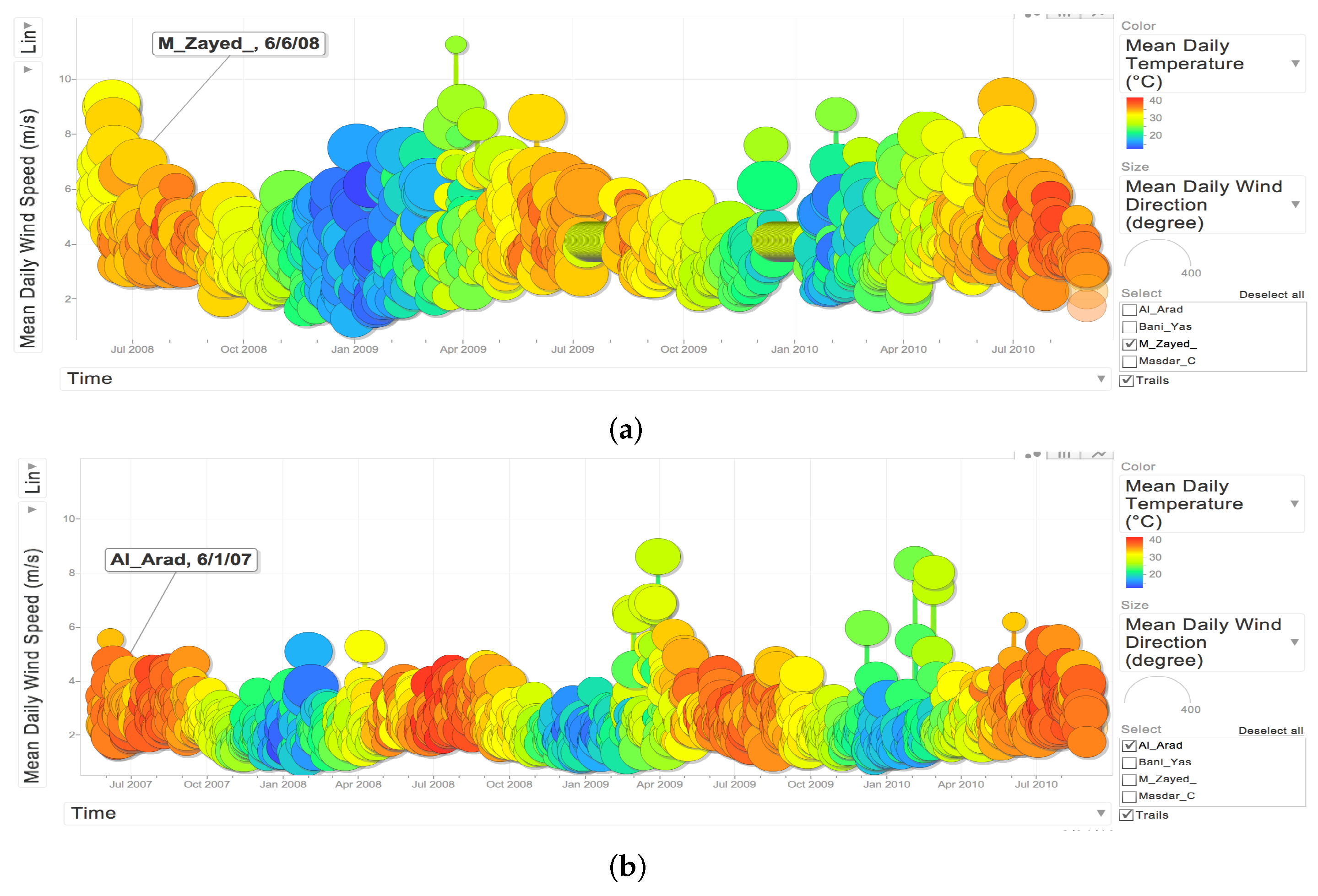
3.1. Data Description and Preliminary Analysis

This subsection deals with the analysis of the correlation between the following meteorological variables: wind speed (WS), wind direction (WD), and temperature (T), measured at two sites, Madinat Zayed and Al Aradh, located in the U.A.E. Formally, we have hourly time series of the WS, WD, and T measured at these sites between:

• 6 June 2008 and 31 August 2010 in Madinat Zayed;
• 1 June 2007 and 31 August 2010 in Al Aradh.

Observe that, even though the wind speed data are observed in different periods for the considered cities, the results will not be affected because the methodology and the predictions are obtained for each site separately. Three types of figures are provided to analyze the intraday correlation between wind speed, wind direction, and temperature. First, a contour plot of hourly wind direction frequencies allows us to find the main wind direction patterns for each station and how they vary during the day. Then, a boxplot of the wind speed for each hour shows how the distribution of the wind speed varies during the day. Finally, a contour plot of wind direction frequencies and the corresponding temperature variation gives an idea about the dependency between the wind direction and temperature.

Now, let us analyze the graphs obtained from Madinat Zayed station. One can observe from the left panel of Figure 2a two main wind direction patterns that happen frequently later in the afternoon: (1) west northwest and (2) northeast. A significant change in the wind speed values occurs around 6 p.m. when the maximum is observed with a median value around 7 m/s. The left panel of Figure 2b shows that a nocturnal cold air comes mainly from the northwest. The highest temperatures are observed when the wind is from the northeast or southwest.

At Al Aradh station, three main prevailing wind directions exist: (1) north northeast, (2) southeast, and (3) west northwest. The left panel of Figure 2c shows a distinct diurnal pattern in these directions with (1) being nocturnal and (2) and (3) denoting the daytime winds. The left panel of Figure 2d shows a cold air frequently observed earlier in the morning and mainly originating from the northeast and the northwest. The highest temperature is observed when the air flow is from the southeast and the southwest. A slight variability in the wind speed distribution is observed earlier in the afternoon.

In order to analyze the time series and check if there is any dependence over time between the wind speed, wind direction, and temperature, we plot the daily average wind speed time series for each station. For instance, Figure 3a shows the evolution of the daily average wind speed over time (days in this figure) at Madinat Zayed station. Each observation of the daily average wind speed process is presented by a circle. The color of the circle is proportional to the measured daily average wind direction, and its color varies with the daily average temperature. Figure 3b displays the daily average wind speed process for Al Aradh station. It is easy to observe a seasonality in the times series. However, the correlation between the daily wind speed, wind direction, and temperature is less easy to observe. For that reason, we will not use the temperature and the wind direction as covariates to predict wind speed. The approaches will, hence, be based only on historical wind speed data.

3.2. An Illustrative Example for the Classification Step: Case of Madinat Zayed

The wind speed time series at Madinat Zayed station was observed at each hour from 6 June 2008 to 31 August 2010. The left panel of Figure 1 shows the original wind speed time series. The right panel of Figure 1 displays the 777 daily wind speed curves denoted by $X_1,X_2,\dots ,X_{777}$. One can observe, from the right panel of Figure 1, that the wind speed starts increasing around 11 a.m. to reach its peak value around 3 p.m., then it decreases to reach lower values from 8 p.m.

The target now consists of providing a single-point forecast of hourly wind speed using as a predictor the conditional median, which corresponds to the conditional quantile of order $\alpha =1/2$. It is well known that the median is more robust than the mean function to the presence of outliers in the sample. In addition to the single-point wind speed forecast, we provide, at each fixed hour r, a conditional predictive interval ${\Xi }_{\alpha }\left(r\right)$.

To validate the approach, we split the sample of 777 daily wind speed curves into two parts. Firstly, for $r=1,\dots ,24$, let $\mathcal{L}=\left\{{(X_1,Y_{1,r})}_r,{(X_2,Y_{2,r})}_r,\dots ,{(X_{412},Y_{412,r})}_r\right\}$ be a learning sub-sample containing daily wind speed curves from 6 June 2008 to 31 August 2009. This sub-sample was used to build clusters and find the optimal bandwidth $h_n$. The second part, denoted as $\mathcal{T}=\left\{{(X_{413},Y_{413,r})}_{r=1,\dots ,24},\dots ,{(X_{777},Y_{777,r})}_{r=1,\dots ,24}\right\}$, is a testing sub-sample, which was used to compare the KS and the CD-KS approaches. In other words, a day-ahead forecast of the daily wind speed curve, as well as an hourly predictive interval were provided between 1 September 2009 and 31 August 2010.

In order to apply the CD-KS approach, we started, as detailed in Section 2.3, by clustering the sample $(X_1,\dots ,X_{412})$ of daily wind speed curves included in the learning sub-sample $\mathcal{L}$. Before applying the classification method, we had to select the tuning parameters represented by the kernel and the semimetric. Since the Madinat Zayed wind curves were not smooth (see Figure 1), we used a semimetric based on the principal component analysis (PCA) of the curves, keeping $q=4$ components, more precisely:

$$d^{PCA}(X_i,X_j):=\sqrt{\sum _{j=1}^q{\langle X_i-X_j,v_j\rangle }^2},$$

where $\langle ·,·\rangle$ denotes the inner product of the space of square integrable functions and $\left(v_j\right)$ denotes the sequence of eigenfunctions of the empirical covariance operator ${\mathsf{\Gamma }}_n$ defined by ${\mathsf{\Gamma }}_{n}u:=n^{-1}{\sum }_{i=1}^n\langle X_i,u\rangle$. The function $K(·)$ was also fixed to be the quadratic kernel defined as $K\left(z\right)=1.5(1-z^2)1{\mathrm{l}}_{[0,1]}$. Then, the application of the descendent hierarchical classification method leads to three clusters.

To observe a common pattern between the clusters’ daily wind speed curves, we used the covariance function defined, for any cluster $m\in \{1,2,3\}$ and $\forall (t,s)\in [0,24)\times [0,24)$, as:

$${\gamma }_{s,t}=\frac{{\sum }_{i=1}^{\overline{{\mathcal{C}}_m}}\left(X_i^{\left(m\right)}\left(t\right)-{\mu }^{\left(m\right)}\left(t\right)\right)\left(X_i^{\left(m\right)}\left(s\right)-{\mu }^{\left(m\right)}\left(s\right)\right)}{\overline{{\mathcal{C}}_m}},$$

where ${\mathcal{C}}_m$ is the m-th cluster, $\overline{{\mathcal{C}}_m}$ is the cardinal number of ${\mathcal{C}}_m$, and ${\mu }^{\left(m\right)}\left(t\right)$ is its mean curve.

Figure 4 displays the obtained covariance function for each cluster. One can see from Figure 4a that a high covariance is observed between 10 a.m. and 5 p.m., which means that the curves that belong to Cluster 1 have a common behavior in this time interval. Figure 4d shows that this common behavior is translated by the increase of the wind speed values from 10 a.m. to reach the unique daily peak around 4 p.m. Figure 4b,c show that Clusters 2 and 3 contain curves with two intra-daily peaks, one that happens in the morning (around 10 a.m.) and the other one in the afternoon (around 5 p.m.). The curves in Cluster 2 are characterized by a high decrease of the wind speed around 5 p.m. One can observe also that, in addition to the difference in the shape of the median profiles, the wind speed level is different between clusters. Curves belonging to Cluster 3 have the highest intra-day wind speed values.

3.3. Choice of the Tuning Parameters for KS and CD-KS Estimators

The estimation of the $\alpha$-th conditional quantiles requires the selection of some tuning parameters, which play an important role in the accuracy of the estimation procedure using either KS or CD-KS. As in the classification step, we considered that the kernel is quadratic and the distribution function $H(·)$ is defined by $H\left(x\right)={\int }_{-\infty }^x\frac{3}{4}(1-t^2)1{\mathrm{l}}_{[-1,1]}\left(t\right)dt$. Moreover, the PCA semimetric was used to measure the closeness between curves. The optimal bandwidth $h_n$ was obtained by the cross-validation method on the $\kappa$-nearest neighbors (see [15], p. 102, for more details).

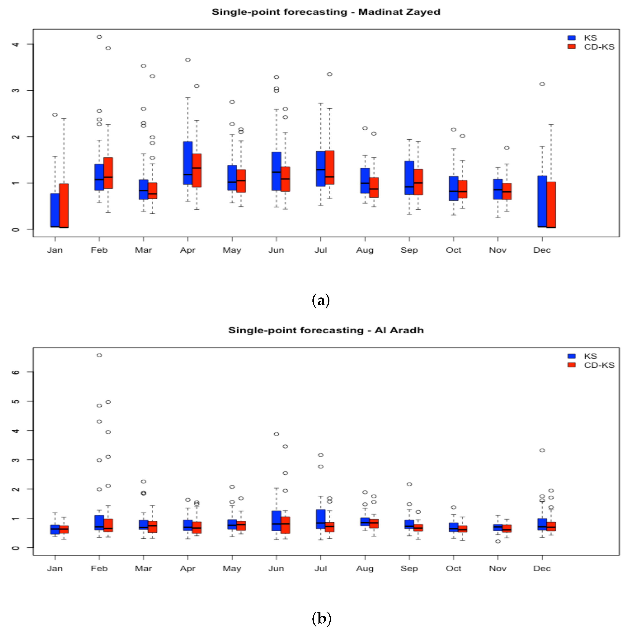
3.4. Validation Procedure and Accuracy Measurements

In this section, we provide the results for single-point hourly wind speed forecasting using as the predictor the conditional median. A 90% conditional hourly predictive interval was also built.

The accuracy of each approach (KS and CD-KS) was measured using hourly and daily errors. For each fixed day, $d=1,\dots ,365$, in the test sample, the hourly absolute errors (HAEs) are defined by:

$${\mathtt{HAE}}_d\left(t_i\right)=|{\widehat{Y}}_{d,t_i}-Y_{d,t_i}|,i=1,\dots ,24,$$

where $Y_{d,t_i}$ is the observed value of the wind speed at day d and hour $t_i$ and ${\widehat{Y}}_{d,t_i}$ is its prediction by the conditional median function. The daily median absolute errors (DMAEs) are defined, for all $d=1,\dots ,365,$ by:

$${\mathtt{DMAE}}_d=\mathtt{Median}\{{\mathtt{HAE}}_d\left(t_1\right),\dots ,{\mathtt{HAE}}_d\left(t_{24}\right)\}$$

Figure 5a,b show the obtained results of the single-point hourly wind speed forecasting errors for Madinat Zayed and Al Aradh stations, respectively. The numerical summary, by month, of the daily median absolute errors is given in

Table 1. Numerical summary of the distribution (by month) of the DMAEs of the hourly wind speed forecasts at Madinat Zayed station obtained by KS and CD-KS.

		KS			CD-KS
	${\mathit{Q}}_{\mathbf{0.25}}$	${\mathit{Q}}_{\mathbf{0.5}}$	${\mathit{Q}}_{\mathbf{0.75}}$	${\mathit{Q}}_{\mathbf{0.25}}$	${\mathit{Q}}_{\mathbf{0.5}}$	${\mathit{Q}}_{\mathbf{0.75}}$
Jan.	0.054	0.054	0.772	0.036	0.036	0.981
Feb.	0.846	1.073	1.388	0.884	1.125	1.497
Mar.	0.646	0.834	1.070	0.660	0.765	1.005
Apr.	0.982	1.182	1.877	0.912	1.322	1.623
May	0.844	1.020	1.381	0.795	1.051	1.288
Jun.	0.850	1.233	1.627	0.821	1.087	1.348
Jul.	0.926	1.286	1.684	0.972	1.131	1.696
Aug.	0.780	0.994	1.320	0.687	0.868	1.116
Sep.	0.753	0.917	1.414	0.745	0.999	1.291
Oct.	0.621	0.822	1.142	0.6753	0.812	1.055
Nov.	0.650	0.855	1.076	0.644	0.807	0.972
Dec.	0.054	0.054	1.155	0.027	0.036	1.023

and

Table 2. Numerical summary of the distribution (by month) of the DMAEs of the hourly wind speed forecasts at Al Aradh station obtained by KS and CD-KS.

		KS			CD-KS
	${\mathit{Q}}_{\mathbf{0.25}}$	${\mathit{Q}}_{\mathbf{0.5}}$	${\mathit{Q}}_{\mathbf{0.75}}$	${\mathit{Q}}_{\mathbf{0.25}}$	${\mathit{Q}}_{\mathbf{0.5}}$	${\mathit{Q}}_{\mathbf{0.75}}$
Jan.	0.460	0.635	0.771	0.491	0.633	0.747
Feb.	0.612	0.707	1.078	0.549	0.651	0.931
Mar.	0.621	0.689	0.936	0.512	0.744	0.904
Apr.	0.583	0.694	0.933	0.505	0.669	0.866
May	0.626	0.762	0.954	0.586	0.784	0.902
Jun.	0.581	0.805	1.223	0.495	0.811	1.019
Jul.	0.649	0.840	1.300	0.538	0.723	0.862
Aug.	0.747	0.850	1.017	0.666	0.843	0.967
Sep.	0.656	0.732	0.931	0.566	0.666	0.787
Oct.	0.546	0.643	0.846	0.527	0.610	0.747
Nov.	0.579	0.704	0.784	0.527	0.606	0.763
Dec.	0.601	0.711	0.991	0.569	0.695	0.869

, respectively. On can observe that the CD-KS approach outperformed KS for the single-point forecasting of hourly wind speed. One can notice from Table 1 and Table 2 that the first, the second, and the third quartiles obtained by CD-KS were in general smaller than those obtained by KS. With respect to the conditional intervals’ prediction, Figure 6 and Figure 7 show that the intervals provided by CD-KS are smaller and much more adapted to the shape of the observed wind speed curve than those obtained by KS. This is clearer when two peaks are observed during the day. This led to the conclusion that the conditioning with respect to the last observed daily wind speed curve is not sufficient, and to mimic the stationarity assumption, we had to proceed first by the classification-discrimination step.

4. Discussion

This paper dealt with the short-term probabilistic forecasting of the hourly wind speed process. The notion of interval prediction introduced in this work allows quantifying the hourly uncertainty of the wind speed. Since the duration of interval predictions is based on the quantile regression notion, an approach based on curve clustering and discrimination was used to deal with the nonstationarity of the wind speed processes. This approach consisted of proceeding first by a classification of the historical daily curves into a fixed number of clusters. Then, using a nonparametric discrimination method, the approach assigns to the last observed curve the corresponding cluster that contains days with a similar shape. The clustering and discrimination steps allow mimicking the stationarity assumption. Finally, the interval, as well as the single-point prediction were produced by applying the kernel-smoothed estimator of the conditional quantile. The application of this approach to hourly wind speed data in the UAE led to accurate single-point forecasts and small interval predictions, which were adapted to the shape of the daily wind speed curve. The obtained point forecasts of the wind speed at different sites can be used to make a decision for selecting the appropriate site or location where the wind turbines should be installed to have the optimal wind power production. Moreover, the probabilistic wind speed prediction established in this paper allows building scenarios of wind power production and consequently gives a better degree of freedom in managing the power network, especially in extreme electricity demand situations. The approach used in this paper was programmed in the R software and can be easily implemented in a real production environment. Note that R is a free software program that is not only commonly used in academia, but it has become, along with Python, one of the most-used software programs in data science and data analytics.

It is worth mentioning that the approach used in this paper is purely nonparametric at the forecasting and classification levels. However, several alternative approaches based on classical parametric time series analysis were used to handle the wind speed point and probabilistic forecasting, as in [5,7]. More recently, approaches based on deep learning models have been used, for instance, in [26,27], where the results were obtained using machine learning algorithms and without assuming an explicit model describing the data. Such approaches are also different from the one we used in this paper, where the conditional quantiles are expressed explicitly. As perspectives on our work, one can include, in addition to the temperature, more predictors, such as the humidity, the historical wind speed curves, and the geographic location, to predict the hourly wind speed. Such an idea could be implemented by modeling the conditional quantiles by some additive functional regression models. One can also adapt the artificial intelligence techniques of the functional data context to predict the wind speed data. Finally, with the progress of technologies, such as sensors, we have more and more access to wind speed data at a very fine time scale. Therefore, the database may become huge in volume (number of observations) and high in the dimension of variables to be used to predict the wind speed. In several situations, the end-user may have storage constraints on the massive data. In such a case, using recursive estimation of conditional quantiles represents an interesting tool to handle massive data and obtain real-time probabilistic wind speed forecasting. In such a case, we do not need to save all the data; we, rather, would update the last value of the forecast by only considering the recently received observation.

References

1. Jeridi Bachellirie, I. Renewable Energy in the GCC Countries. Resources, Potential, and Prospects; Gulf Research Center: Dubai, United Arab Emirates, 2012. [Google Scholar]
2. Sanchez, I. Short term prediction of wind energy production. Int. J. Forecast. 2006, 22, 43–56. [Google Scholar] [CrossRef]
3. Zhao, P.; Wang, J.; Xia, J.; Dai, Y.; Sheng, Y.; Yue, J. Performance evaluation and accuracy enhancement of a day-ahead wind power forecasting system in china. Renew. Energy 2012, 43, 234–241. [Google Scholar] [CrossRef]
4. Liu, H.; Tian, H.; Pan, D.; Li, Y. Forecasting models of wind speed using wavelet, wavelet packet, time series and artificial neural networks. Appl. Energy 2013, 107, 191–208. [Google Scholar] [CrossRef]
5. Salcedo-Sanz, S.; Ortiz-Garcá, E.G.; Pérez-Bellido, Á.M.; Portilla-Figueras, A.; Piereto, L. Short term wind speed prediction based on evolutionary support vector regression algorithms. Expert Syst. Appl. 2006, 38, 4052–4057. [Google Scholar] [CrossRef]
6. Poggi, P.; Muselli, M.; Notton, G.; Cristofari, C.; Louche, A. Forecasting and simulating wind speed in Corsica by using an autoregressive model. Energy Convers. Manag. 2003, 44, 3177–3196. [Google Scholar] [CrossRef]
7. Kavasseri, R.; Seetharaman, G. Day-ahead wind speed forecasting using f-ARIMA models. Renew. Energy 2009, 34, 1388–1393. [Google Scholar] [CrossRef]
8. Ailliot, P.; Monbet, V.; Prevosto, M. An autoregressive model with time-varying coefficients for wind fields. Environmetrics 2006, 17, 107–117. [Google Scholar] [CrossRef]
9. Hocaoglua, F.O.; Gerekb, Ö.N.; Kurbanb, M. A novel wind speed modeling approach using atmospheric pressure observations and hidden Markov models. J. Wind. Eng. Ind. Aerodyn. 2010, 98, 472–481. [Google Scholar] [CrossRef]
10. D’Amico, G.; Petroni, F.; Prattico, F. Wind speed modeled as an indexed semi-Markov process. Environmetrics 2013, 24, 367–376. [Google Scholar] [CrossRef]
11. Moldernik, A.; Bakker, V.; Bosman, M.; Hurink, J.; Smit, G. Management and control of domestic smart grid technology. IEEE Trans. Smart Grid 2010, 1, 109–119. [Google Scholar] [CrossRef]
12. Ouammi, A.; Dagdougui, H.; Sacile, R. Optimal planning with technology selection for wind power plants in power distribution networks. IEEE Syst. J. 2019, 13, 3059–3069. [Google Scholar] [CrossRef]
13. Ouammi, A.; Ghigliotti, V.; Robba, M.; Mimert, A.; Sacile, R. A decision support system for the optimal exploitation of wind energy on regional scale. Renew. Energy 2012, 37, 299–309. [Google Scholar] [CrossRef]
14. Ramsay, J.O.; Silverman, B.W. Functional Data Analysis, 2nd ed.; Springer Series in Statistics; Springer: New York, NY, USA, 2005. [Google Scholar]
15. Ferraty, F.; Vieu, P. Nonparametric Functional Data Analysis: Theory and Practice; Springer Series in Statistics; Springer: New York, NY, USA, 2006. [Google Scholar]
16. Chaouch, M. Clustering-based improvement of nonparametric functional time series forecasting. Application to intraday household-level load curves. IEEE Trans. Smart Grid 2013, 99, 411–419. [Google Scholar] [CrossRef]
17. Rice, J.A. Functional and longitudinal data analysis: Perspectives on smoothing. Stat. Sin. 2004, 14, 631–647. [Google Scholar]
18. Yao, Q.; Tong, H. On prediction and chaos in stochastic systems. Philos. Trans. R. Soc. A 1994, 348, 357–369. [Google Scholar] [CrossRef]
19. De Gooijer, J.G.; Gannoun, A. Nonparametric conditional predictive regions for time series. Comput. Stat. Data Anal. 2000, 33, 259–275. [Google Scholar] [CrossRef]
20. Chaouch, M.; Khardani, S. Randomly censored quantile regression estimation using functional stationary ergodic data. J. Nonparametric Stat. 2015, 21, 65–87. [Google Scholar] [CrossRef]
21. Wand, M.P.; Jones, M.C. Kernel Smoothing; Chapman & Hall: London, UK, 1995. [Google Scholar]
22. Simonoff, J. Smoothing Methods in Statistics; Springer: New York, NY, USA, 1996. [Google Scholar]
23. Cuesta-Albertos, J.; Fraiman, R. Impartial trimmed k-means and classification rules for functional data. Comput. Stat. Data Anal. 2007, 51, 4864–4877. [Google Scholar] [CrossRef]
24. Dabo-Niang, S.; Ferraty, F.; Vieu, P. Mode estimation for functional random variable and its application for curves classification. Far East J. Theor. Stat. 2006, 18, 93–119. [Google Scholar]
25. Ferraty, F.; Vieu, P. Curves discrimination: A nonparametric functional approach. Comput. Stat. Data Anal. 2003, 44, 161–173. [Google Scholar] [CrossRef]
26. Lin, Y.; Qin, H.; Zhang, Z.; Pei, S.; Jiang, Z.; Feng, Z.; Zhou, J. Probabilistic spatiotemporal wind speed forecasting based on a variational bayesian deep learning model. Appl. Energy 2020, 260, 114259. [Google Scholar]
27. Jiang, Y.; Zhao, N.; Peng, L.; Lin, S. A new hybrid framework for probabilistic wind speed prediction using deep feature selection and multi-error modification. Energy Convers. Manag. 2019, 199, 111981. [Google Scholar] [CrossRef]
Figure 1. The hourly wind speed process ξ ( t ) observed at Madinat Zayed station between 16 July 2008 and 31 August 2010 (left) and the corresponding smoothed functional data ( X i ( t ) ) i = 1 , , n (right).
Energies 16 07615 g001
Figure 2. Left panel: hourly wind direction frequencies and the corresponding hourly wind speed distribution for Madinat Zayed (a) and Al Aradh (c). Right panel: hourly wind direction frequencies and their temperature variation and the corresponding hourly wind speed distribution for Madinat Zayed (b) and Al Aradh (d).
Energies 16 07615 g002
Figure 3. Daily average wind speed process observed at Madinat Zayed (a) and Al Aradh (b).
Energies 16 07615 g003
Figure 4. Covariance function of daily wind speed curves for Cluster 1 (respectively, 2 and 3) is plotted in (a) (respectively, (b,c)). Median wind speed profiles for each cluster are plotted in (d).
Energies 16 07615 g004
Figure 5. Distribution (by month) of the daily median absolute errors (DMAEs) obtained by KS and CD-KS for Madinat Zayed (a) and Al Aradh (b).
Energies 16 07615 g005
Figure 6. Hourly interval prediction, obtained by the CD-KS (left boxes) and KS (right boxes) methods, for two randomly sampled days in the test sample of Madinat Zayed station.
Energies 16 07615 g006
Figure 7. Hourly interval prediction, obtained by the CD-KS (left boxes) and KS (right boxes) methods, for two randomly sampled days in the test sample of Al Aradh station.
Energies 16 07615 g007