A Dynamic Nonlinear VDCOL Control Strategy Based on the Taylor Expansion of DC Voltages for Suppressing the Subsequent Commutation Failure in HVDC Transmission

Abstract

Subsequent commutation failure in high-voltage DC transmission systems seriously emphasizes the safe and stable operation of power systems. Via analyzing the mechanism of commutation failure and the principle of voltage-dependent current order limiter (VDCOL), this paper proposes a dynamic nonlinear VDCOL control strategy based on the Taylor expansion of DC voltage for suppressing subsequent commutation failure. To solve the problem of fluctuating DC current command value caused by a large drop in DC voltage, this paper constructs a nonlinear VDCOL control that can be dynamically adjusted according to the AC bus voltage level, and Taylor expansion of DC voltage is used to obtain its first-order and second-order differential components. Different scales of differential elements are chosen to predict the DC voltage compensation value while balancing sensitivity and accuracy. The compensated DC voltage, used as the starting voltage of VDCOL, is input to the VDCOL control constructed in this paper to suppress the subsequent commutation failure of the transmission system by reducing the fluctuation of the current command value. Finally, the standard test model of HVDC is established based on the actual parameters, and the simulation results show that the Method proposed in this paper has an effective suppressing effect in the case of single-phase or three-phase faults of different severity and is conducive to the restoration of the system power transmission.

1. Introduction

Due to the imbalance between the distribution of energy and energy consumption in China formed the pattern of electricity transmission from the West to the East. Line-Commutated-Converter High Voltage Direct Current (LCC-HVDC) has developed rapidly due to the advantages of larger transmission capacity, longer transmission distance, less cost, and smaller line loss, etc. [1]. The thyristor is the basic component of the commutation station of an HVDC transmission system, which is prone to the problem of commutation failure due to bus faults because of its lack of autonomous shutdown capability [2]. The thyristor’s service life will be shortened by commutation failure, which will also result in a considerable rise in DC current and a decrease in the system’s power transfer efficiency. When corrective action is taken following a single commutation failure, the DC system can usually be recovered on its own. However, if the recovery process is repeated for subsequent commutation failures, it will exacerbate the effects on the AC system and, in extreme circumstances, result in DC system blocking and transmission power interruption, which puts the power system’s ability to operate safely and steadily in jeopardy [3]. Thus, in the fault recovery process, the following commutation failure is more significant than the initial commutation failure.

Scholars at home and abroad have carried out a large number of studies on the problem of commutation failure. Ref. [4] analyses the relationship between the AC bus, trigger delay angle of LCC, the ratio of converter transformer, DC current, and other factors and inverter extinction angle, as well as the impact on the commutation failure, and put forward corresponding suppressing measures. Existing Methods to suppress commutation failure can be divided into two main categories: modifying the system topology and optimizing the protection control strategy. In terms of modifying the system topology, Refs. [5,6] changes the inverter topology by connecting power electronic devices in series and parallel at the inverter, thus reducing the risk of commutation failure. Ref. [7] proposes a new type of controllable line commutated converter (CLCC) topology with controllable shutdown capability based on the design idea of mixing full-control and half-control devices, but the main branch IGBT through-current is too large, and the total valve loss increases. Ref. [8] proposes a scheme to form a flexible LCC system by connecting a cascaded H-bridge in series between a grid commutation converter and a converter transformer. Ref. [9] improves the transient voltage stability level of AC bus voltage by adding reactive power compensation equipment to the system. Ref. [10] uses the magnitude of reactive power output from the STATCOM to measure the degree of DC system recovery and combines the reactive power output from the STATCOM and the DC voltage as the input signal to the VDCOL, combining the features of changing the system topology and optimizing the system control strategy. However, the above Methods have the problems of higher system construction cost, limited voltage level and transmission capacity, and more difficult practical application. The control strategy of the system can be optimized in several ways. Based on the theory of time-integrated area of commutation voltage, Ref. [11] proposes the theory of pulse-advance triggering control to increase the commutation area and reduce the probability of commutation failure occurring in the system. Ref. [12] based on the proposed pseudo-commutation process, a pseudo-extinction angle prediction module is specially designed to adjust the extinction angle sequence in time with real-time, but the harmonic voltages are irregular and unpredictable, which makes it difficult to accurately predict and adjust the phase-commutation sequence. Ref. [13] considers the basis of harmonic parts and combines the correction margin with the rate of change of voltage to obtain the compensation margin of the lagging trigger angle, but the suppression effect under some fault times is not satisfactory enough. The trigger angle deviation compensation-based control scheme proposed in Ref. [14] can effectively inhibit the occurrence of continuous phase change failure by restricting the trigger angle command, but this measure only works on phase change failure under single-phase faults, and its applicability is narrow. Ref. [15] increases the system commutation capability by limiting the DC current during trigger angle overshoot, but the system reactive power support capability is poor, and the system power fluctuation is serious. Ref. [16] proposes an adaptive control of phase lock oscillator (PLO) that captures the rapid changes in commutation voltage, provides more accurate phase information during fault recovery, and speeds up system recovery. It is applicable in light faults, nevertheless insignificant effect in heavy faults. Ref. [17] increases the system phase change capability by limiting the DC current during trigger angle overshoot, but the system reactive power support capability is poor, and the system power fluctuation is serious. Ref. [18] regard harmonic-induced commutation voltage distortion as the main cause of commutation failure, based on commutation failure prevention (CFPREV), according to the harmonic component of commutation voltage and the rate of change of AC bus voltage, thus increasing the commutation margin and reducing the chances of commutation failure occurring.

The voltage-dependent current order limiter (VDCOL) is an important part of the HVDC transmission system to suppress continuous commutation failure due to its simple principal structure [19]. Ref. [20] analyses the principle of VDCOL suppression to suppress continuous commutation failure, whereas it is difficult to respond quickly to continuous commutation failure due to the low sensitivity of the conventional VDCOL. Refs. [21,22] proposes the Method of changing the upper limit value of the system DC voltage, which can give full play to the fast controllability of DC voltage and improve the stability level of the system, but it does not take into consideration the change of the extinction angle in the process of fault recovery, which leads to the unsatisfactory effect of suppressing the failure of commutation. Ref. [23] combines the advantages of AC and DC starting voltages to design an AC/DC-VDCOL conversion coordination controller, but the small sensitivity of VDCOL makes it difficult to suppress the continuous phase change failure under heavy faults. Ref. [24] analyzes the successive commutation failures from the current deviation control link and designs the restricted low-voltage current limiting link to improve the cooperation between the low-voltage current limiting control and the current deviation control. Ref. [25] adopts the virtual phase change voltage difference startup criterion, the reasonable triggering of inverter-side overrun angle, combined with the rectifier-side feed-forward link, which is affected by the time delay, to effectively inhibit the phase change failure based on reducing the time delay. Refs. [26,27,28] proposed the concept of virtual resistance, virtual inductance, and virtual capacitance to optimize the starting voltage of the VDCOL to improve the response speed of the VDCOL, but the conventional VDCOL control is used; as a result, it is more difficult to recover the DC delivered power in case of a system with a heavy fault. Ref. [29] proposes a predictive VDCOL control strategy that obtains the amount of current variation by Taylor unfolding the DC current and combines it with a virtual resistance. Ref. [30] proposes the control Method to obtain the compensation voltage to change the slope of VDCOL to meet the active and reactive power requirements of the transmission system during phase change failures and restoration. Ref. [31] proposes a control strategy on nonlinear VDCOL, which improves the sensitivity of the DC command current but is not responsive to mild to moderate faults. Ref. [32] combines virtual capacitance and nonlinear VDCOL control strategies to improve the sensitivity of the system response to faults, but it does not take into consideration the process of fault recovery, which leads to too slow fault recovery. Ref. [33] changed the VDCOL control structure based on the introduction of fuzzy control theory, which effectively reduced the reactive power demand of the inverter. Ref. [34] divides the process of voltage recovery into different stages and sets different recovery rates thus improving the system power transfer performance. Among the existing studies on VDCOL improvement, the reference optimized the starting voltage of VDCOL via virtual components to reduce the fluctuation of current command but did not consider the influence of the recovery speed of the current command on the fault recovery process, resulting in too slow recovery of the system power. The reference constructed a dynamic nonlinear VDCOL control strategy, but it did not optimize the startup voltage, causing the DC command value to fluctuate drastically, rendering it ineffectual under heavy fault circumstances. Based on the above study, this paper proposes a dynamic nonlinear VDCOL control strategy based on the Taylor expansion of DC voltages for suppressing the subsequent commutation failure in HVDC transmission by proposing a new optimization Method of startup voltage and constructing a VDCOL that considers the current command of the fault recovery process on the system recovery, which accelerates the recovery of the system power transfer while increasing the coverage range of suppression of phase change failure.

Among the existing studies on VDCOL improvement, Refs. [26,27,28] optimized the starting voltage of VDCOL via virtual components to reduce the fluctuation of the current command but did not consider the influence of the recovery speed of the current command on the fault recovery process, resulting in the too-slow recovery of the system power. Refs. [30,31,32] constructed a dynamic nonlinear VDCOL control strategy, but it did not optimize the startup voltage, causing the DC command value to fluctuate drastically, rendering it ineffectual under heavy fault circumstances. Based on the above study, this paper proposes a dynamic nonlinear VDCOL control strategy based on the Taylor expansion of DC voltages for suppressing the subsequent commutation failure in HVDC transmission by proposing a new optimization Method of startup voltage and constructing a VDCOL that considers the current command of the fault recovery process on the system recovery, which accelerates the recovery of the system power transfer while increasing the coverage range of suppression of phase change failure.

Based on the research above, this article is divided into six parts. Section 2 analyses the mechanism of phase commutation failure and the working principle of VDCOL. It concludes that the drastic fluctuation of DC current command, due to the large drop in DC voltage, is the key reason for subsequent commutation failure. It also proposes a dynamic nonlinear VDCOL control strategy based on the Taylor expansion of DC voltage. In Section 3, the DC voltage variation is obtained using Taylor expansion to optimize the starting voltage of VDCOL. In Section 4, a dynamic nonlinear VDCOL is constructed to dynamically adjust the DC current command based on the AC bus voltage. In Section 5, a simulation model is built using the actual data to verify the effectiveness of the proposed Method in this paper. Finally, the conclusions of our work are presented in Section 6.

2. The Commutation Failure and VDCOL Control

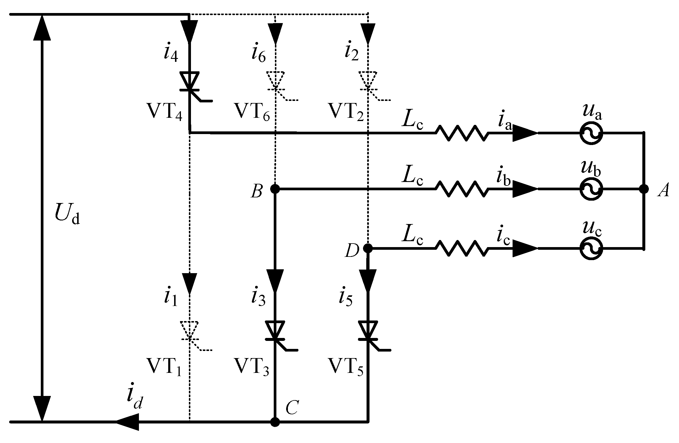
2.1. Analysis of the Commutation Failure

The commutation failure is the most common fault of the inverter. As shown in Figure 1, the simple model of the commutation process is shown to analyze the inverter commutation process from inverter valve $\mathrm{V}{\mathrm{T}}_3$ to $\mathrm{V}{\mathrm{T}}_5$. Before the commutation, the inverter valves $\mathrm{V}{\mathrm{T}}_3$ and $\mathrm{V}{\mathrm{T}}_4$ connect to form a circuit. After receiving the trigger pulse, the inverter valve $\mathrm{V}{\mathrm{T}}_5$ is energized. There are three converter valves that turn on in the inverter until the current $i_3$ flowing through the valve $\mathrm{V}{\mathrm{T}}_3$ decreases to zero.

As shown in Figure 1, $i_3$, and $i_5$ are the currents flowing through commutator valves $\mathrm{V}{\mathrm{T}}_3$ and $\mathrm{V}{\mathrm{T}}_5$ respectively, $i_d$ is the commutation current, and $L_c$ is the equivalent phase change reactance. The rest of the commutator valves remain closed.

During the phase change, the BC phases are operated in parallel. According to Kirchhoff’s voltage law, the voltage relationship is as follows:

$$L_c\frac{d{i}_3}{dt}+U_b=L_c\frac{d{i}_5}{dt}+U_c$$

(1)

Then:

$$L_c\frac{d{i}_5}{dt}-L_c\frac{d{i}_3}{dt}=\sqrt{2}E\sin \omega t$$

(2)

where $E$ is the inverter-side AC bus voltage RMS value. $\omega$ is the AC system angular frequency.

In the commutation process, according to Kirchhoff’s current law, the current satisfies the following relationship:

$$i_d=i_3+i_5$$

(3)

This can be obtained by substituting (3) into (2) and integrating both sides simultaneously:

$$2L_c{I}_d=\sqrt{2}{\displaystyle {\int }_{\alpha }^{\alpha +\mu }E\sin \omega tdt}$$

(4)

In the equation: $\alpha$ is the inverter firing angle, and $\mu$ is the inverter commutation angle.

Define the inverter commutation demand area $S_{need}$ as:

$$S_{need}=2L_c{I}_d$$

(5)

Define the maximum commutation area $S_{max}$ available from the system as:

$$S_{\max }=\sqrt{2}{\displaystyle {\int }_{\alpha }^{\alpha +\mu }E\sin \omega tdt}$$

(6)

During the commutation process, when the inverter commutation demand area $S_{need}$ is larger than the maximum commutation area $S_{max}$ that the system can provide, the practical inverter extinction angle $\gamma$ is smaller than the minimum inverter extinction angle ${\gamma }_{min}$, resulting in insufficient commutation time margin, making it difficult for the thyristor to recover its blocking capability, and thus, the system fails to commute for the first time. If appropriate suppression measures are not taken, the first commutation failure can easily cause subsequent commutation failures, seriously endangering the safe and stable operation of the system. Numerous research has shown that the first commutation failure acts for a short period, so it is difficult to avoid, while the subsequent commutation failure subsequently acts for a long period, and the electrical quantity of the system changes drastically, which causes a serious shock to the system. Thus, the system has enough time to react to subsequent commutation failures subsequently. Therefore, it is more meaningful and feasible to suppress subsequent commutation failures for the stability of HVDC transmission systems.

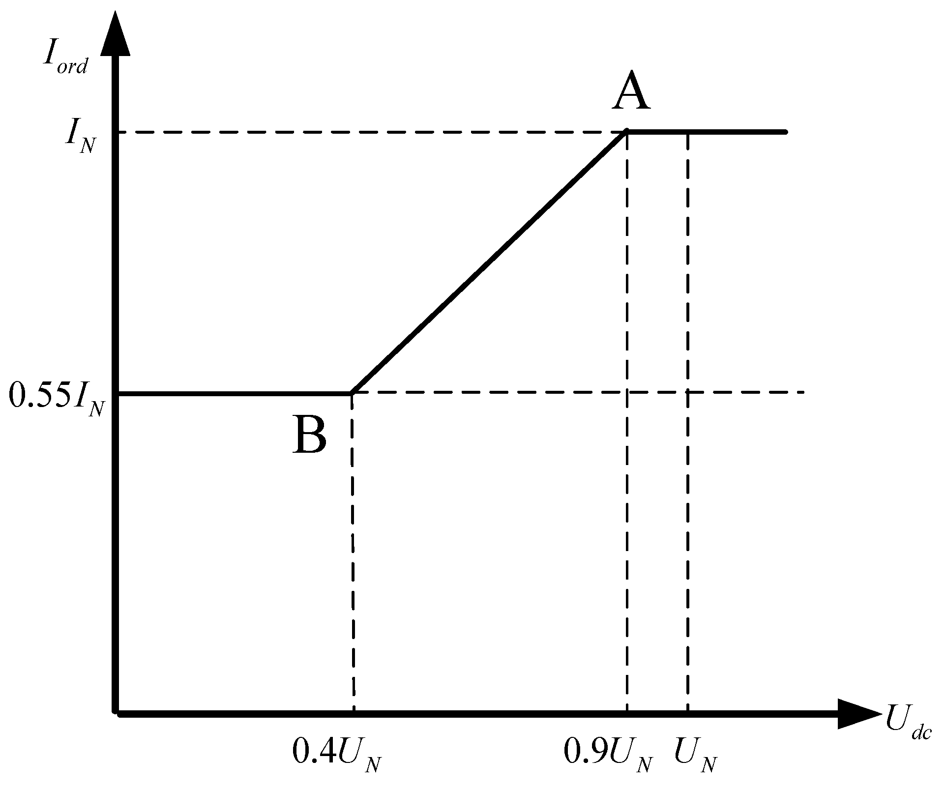
2.2. VDCOL and the Commutation Failures

In the HDVC transmission system, VDCOL is an important part of suppressing the failure of system commutation. The ground-to-ground voltage at the midpoint of the DC line of the inverter is used as the starting voltage of the VDCOL. When the system voltage drops rapidly to a certain value during an AC system bus failure at the inverter side, the VDCOL starts and temporarily restricts the DC current by reducing current commands to reduce the reactive power loss, thus facilitating the recovery of the AC bus voltage.

The operating characteristic curve of the normal VDCOL is shown in Figure 2, where the relationship between the DC voltage $U_{dc}$ and the DC current command value $I_{ord}$ is as follows:

$$I_{ord}=\left\{\begin{array}{cc}0.55 \mathrm{p.u.}& U_{dc}<0.4 \mathrm{p.u.}\\ 0.9U_{dc}+0.19 \mathrm{p.u.}& 0.4 \mathrm{p.u.}\le U_{dc}\le 0.9 \mathrm{p.u.}\\ 1 \mathrm{p.u.}& U_{dc}>0.9 \mathrm{p.u.}\end{array}\right.$$

(7)

A fault occurs in the inverter-side AC bus, resulting in a sharp increase in DC current and a rapid drop in system voltage to $U_{dc}=0.9 \mathrm{p.u.}$, thus, the VDCOL will start up. As shown in Figure 2, VDCOL activated at Point A, power transfer maintained at Point B. However, due to the linear relationship between voltage and current of the normal VDCOL, the fixed slope of the VDCOL curve results in a low sensitivity of the DC current command. As a result, the current command value of the normal VDCOL output is difficult to match the fault severity enough to come quickly enough to reduce the DC current, resulting in the first commutation failure. During the fault recovery period, the system voltage drops and rises rapidly, which causes the current command of VDCOL output to fluctuate drastically. Further, the area required for inverter commutation is larger than the maximum area provided by the system for commutation, which leads to subsequent commutation failures.

3. DC Voltage Compensation Based on Taylor’s Equation

According to the previous analysis, the drastic fluctuation of the current command in VDCOL is the key reason for the subsequent commutation failure in HVDC transmission systems. When a ground fault occurs in the AC bus, the system voltage falls sharply, and the VDCOL output current command value fluctuates dramatically, increasing the risk of subsequent commutation failure. Therefore, Taylor expansion of the inverter-side DC voltage is performed to predict the DC voltage trend according to the DC voltage trend. During the bus fault occurrence, the predicted inverter-side DC voltage variation is compensated into the falling DC voltage, used as the starting voltage of the VDCOL. By reducing the DC voltage dip, fluctuations of the VDCOL output current command are reduced with the result of suppressing subsequent commutation failures in turn.

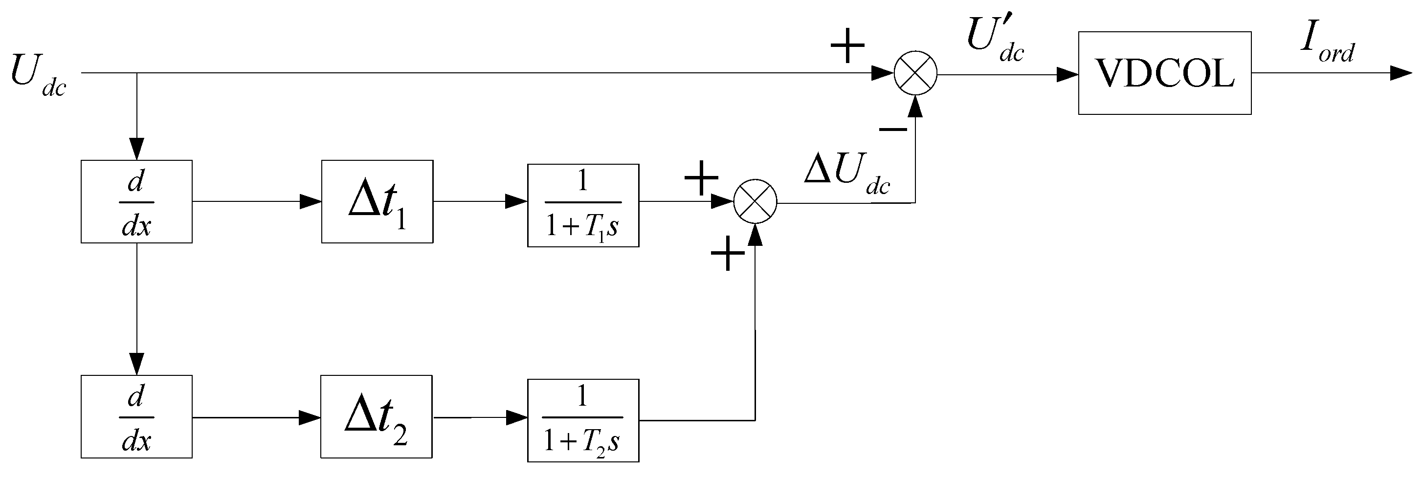
3.1. Compensation Based on the Change of DC Voltage

When $t=t_0$, the Taylor expansion of the inverter-side DC voltage is

$$U_{di}(t)=\frac{U_{di}\left(t_0\right)}{0!}+\frac{U_{di}{}^{\prime }\left(t_0\right)}{1!}\left(t-t_0\right)+\frac{U_{di}{}^{″}\left(t_0\right)}{2!}{\left(t-t_0\right)}^2+\dots +\frac{U_{di}{}^{(n)}\left(t_0\right)}{n!}{\left(t-t_0\right)}^n+R_n(t)$$

(8)

A commutation period is 20 ms, and the inverter extinction angle corresponds to a time of about 2 ms. To predict the DC voltage by Taylor expansion of the DC voltage on the inverter side, the time step $\mathsf{\Delta }t=t-t_0$ has to be small enough to be milliseconds. Since the DC voltage differentials of third order and above are then exceedingly small, to simplify the calculation, the DC voltage expansion equation is obtained by neglecting the third order and above differential terms and residual terms:

$$U_{di}(t)=U_{di}(t_0)+\frac{\mathrm{d}{U}_{di}(t_0)}{\mathrm{d}t}(t-t_0)+\frac{{\mathrm{d}}^2{U}_{di}(t_0)}{\mathrm{d}{t}^2}\frac{{(t-t_0)}^2}{2}$$

(9)

The change of DC voltage $\mathsf{\Delta }{U}_{di}$ during the prediction time $\mathsf{\Delta }t$ is:

The first-order differential and the second-order differential in the DC voltage variation have different roles in the compensation of the DC voltage. The first-order differential can predict the change in voltage value after time $t_0$ according to the rate of change of DC voltage, which plays a major role in the prediction. The second-order differential term is a correction to the DC voltage prediction based on the rate of change of the DC voltage rate of change to further improve the sensitivity and accuracy. If the time step is too small, the first-order differential is small, and its sensitivity is insufficient, resulting in the prediction effect being limited; if the time step $\mathsf{\Delta }t$ is too large, the harmonics brought by the second-order differential will deteriorate the prediction accuracy.

Since different values of the time step $\mathsf{\Delta }t$ can have an important effect on the system to suppress commutation failure. Therefore, to consider both the sensitivity and accuracy of the system, the time steps $\mathsf{\Delta }t$ of the first-order differential and second-order differential terms at the DC voltage are taken to be different values. Define the time step of the first-order differential as the prediction parameter $\mathsf{\Delta }{t}_1$, and define the time step of the second-order differential as the correction parameter $\mathsf{\Delta }{t}_2$.

$$\Delta U_{di}=\frac{\mathrm{d}{U}_{di}(t_0)}{\mathrm{d}t}\Delta t_1+\frac{{\mathrm{d}}^2{U}_{di}(t_0)}{\mathrm{d}{t}^2}\frac{\Delta t_2{}^2}{2}$$

(10)

By subtracting the voltage variation $\mathsf{\Delta }{U}_{di}$ from the initial DC voltage value $U_{di}$, the compensated DC voltage value $U_{dc}$ can be obtained and used as the input voltage to the VDCOL:

$$U_{dc}=U_{di}-\Delta U_{di}$$

(11)

In the event of a ground fault at the AC bus leading to a drop in the voltage of the system, the change of voltage $\mathsf{\Delta }{U}_{di}<0$. The starting voltage $U_{dc}$ is greater than the inverter-side DC voltage $U_{di}$, which eliminates the falling DC voltage factor, optimizes the VDCOL starting voltage, and reduces the fluctuations of DC current command, thus effectively suppressing subsequent commutation failure. The optimization of the starting voltage in VDCOL is shown in Figure 3.

3.2. Predictive Parameters Analyzed and Determined

The purpose of this section is to analyze the effect of different values of the prediction parameter $\mathsf{\Delta }{t}_1$ on suppressing the failure of the system commutation. The prediction parameter $\mathsf{\Delta }{t}_1$ plays an important role in predicting the amount of DC voltage change. The larger the prediction parameter $\mathsf{\Delta }{t}_1$ is, the more sensitive the prediction function is. In the same time range, the prediction parameter $\mathsf{\Delta }{t}_1$ can be used to provide a larger amount of compensation for the DC voltage change so as to reduce the DC voltage drop, effectively suppress the subsequent commutation failure, and accelerate the system recovery.

Three-phase ground faults through different sizes of inductive are setting up grounding at the AC bus at the inverter side. The moment of fault occurrence at 1.0 s, and the fault lasts for 0.5 s. Set $\mathsf{\Delta }{t}_2=0 \mathrm{s}$, respectively, different values of prediction parameter $\mathsf{\Delta }{t}_1$ are selected, and the recovery time of commutation failure of the system is counted and the statistical results are shown in

Table 1. Recovery time of commutation failure at $\mathsf{\Delta }{t}_1$.

Ground Inductance/H	Recovery Time of Commutation Failure/s
	0 ms	5 ms	10 ms	15 ms	20 ms
0.1	0.098	0.059	0.032	0.039	0.032
0.2	0.037	0.037	0.042	0.039	0.039
0.3	0.063	0.037	0.039	0.039	0.039
0.4	0.063	0.083	0.064	0.039	0.064
0.5	0.08	0.064	0.062	0.039	0.077
0.6	0.083	0.08	0.08	0.039	0.08
0.7	0.093	0.065	0.081	0.061	0.08
0.8	0.093	0.073	0.071	0.071	0.085
0.9	0.073	0.074	0.047	0.047	0.073
1.0	0.084	0.084	0.084	0.063	0.084
Sum-up time/s	0.767	0.656	0.602	0.476	0.653

.

From Table 1, the effect of different prediction parameters $\mathsf{\Delta }{t}_1$ on the recovery time of commutation failure, it can be seen that when a three-phase ground fault occurs on the inverter side, the normal control Method $\mathsf{\Delta }{t}_1=0 \mathrm{m}\mathrm{s}$ is unable to effectively suppress the subsequent commutation failure of the system in the case of a more serious short-circuit fault, which leads to a longer time required for the recovery of the system, and the sum-up recovery time of the commutation failure is 0.767 s. After adding the DC voltage first-order differential, the VDCOL starting voltage is optimized. The sum-up recovery time of the system commutation failure is significantly shorter than the original time, which can effectively suppress the subsequent commutation failure. Within a certain time range, increasing the step size of the prediction parameter $\mathsf{\Delta }{t}_1$ can decrease the system commutation failure recovery time and improve the suppressing effect of subsequent commutation failure. However, if the prediction parameter $\mathsf{\Delta }{t}_1$ is too large, the fluctuation of the compensation value of the DC voltage change will be too large, leading to the intensification of harmonic effects and thus worsening the suppressing effect. Therefore, based on the statistical results in Table 1, the prediction parameter $\mathsf{\Delta }{t}_1=15 \mathrm{m}\mathrm{s}$.

3.3. Correction Parameters Analyzed and Determined

The purpose of this section is to analyze the effect of different values of the correction parameter on suppressing the commutation failure of the system. The correction parameter $\mathsf{\Delta }{t}_2$ acts as a correction for the change of DC voltage, thus improving the accuracy of the control Method. Since the correction parameter $\mathsf{\Delta }{t}_2$ acts on the second-order differentiation, which introduces a harmonic influence. The harmonic frequency increases as the differential order increases. The larger the harmonic frequency, the more unfavorable not only is it to suppress the failure of commutation, but at the same time, it will also be harmful to the safe and stable operation of the power system. Therefore, the correction parameter $\mathsf{\Delta }{t}_2$ is set in milliseconds in order to reduce the generation of harmonics.

Three-phase ground faults through different sizes of inductive are setting up grounding at the AC bus at the inverter side. The moment of fault occurrence is 1.0 s, and the fault lasts for 0.5 s. Set $\mathsf{\Delta }{t}_1=15 \mathrm{ms}$, respectively, different values of correction parameter $\mathsf{\Delta }{t}_2$ are selected, and the recovery time of commutation failure of the system is counted and the statistical results are shown in

Table 2. Recovery time of commutation failure at $\mathsf{\Delta }{t}_2$.

Ground Inductance/H	Recovery Time of Commutation Failure/s
	1 ms	2 ms	3 ms	4 ms	5 ms
0.1	0.032	0.032	0.032	0.032	0.032
0.2	0.039	0.042	0.042	0.042	0.042
0.3	0.039	0.039	0.039	0.039	0.039
0.4	0.039	0.039	0.039	0.039	0.039
0.5	0.039	0.039	0.039	0.039	0.039
0.6	0.039	0.039	0.039	0.039	0.039
0.7	0.039	0.039	0.039	0.039	0.039
0.8	0.047	0.047	0.047	0.047	0.047
0.9	0.071	0.047	0.047	0.047	0.071
1.0	0.062	0.063	0.067	0.079	0.079
Sum-up time/s	0.446	0.426	0.43	0.442	0.466

.

From Table 2, the effect of different correction parameters $\mathsf{\Delta }{t}_2$ on the recovery time of commutation failure, it can be seen that, within a certain time range, the accuracy of the control Method can be improved with the increase in correction parameters $\mathsf{\Delta }{t}_2$, shortening the sum-up time of system commutation failure, which can suppress the subsequent commutation failure effectively. When the correction parameter is $\mathsf{\Delta }{t}_2$, the sum-up recovery time for system commutation failure is the shortest, and the effect of suppressing subsequent commutation failures is the most significant. However, as the correction parameter $\mathsf{\Delta }{t}_2$ continues to increase, the amplitude of the voltage harmonics brought about by the second-order differential also increases, which can deteriorate the suppression of commutation failure. Therefore, according to the statistical results in Table 2, the correction parameter $\mathsf{\Delta }{t}_2=2 \mathrm{m}\mathrm{s}$.

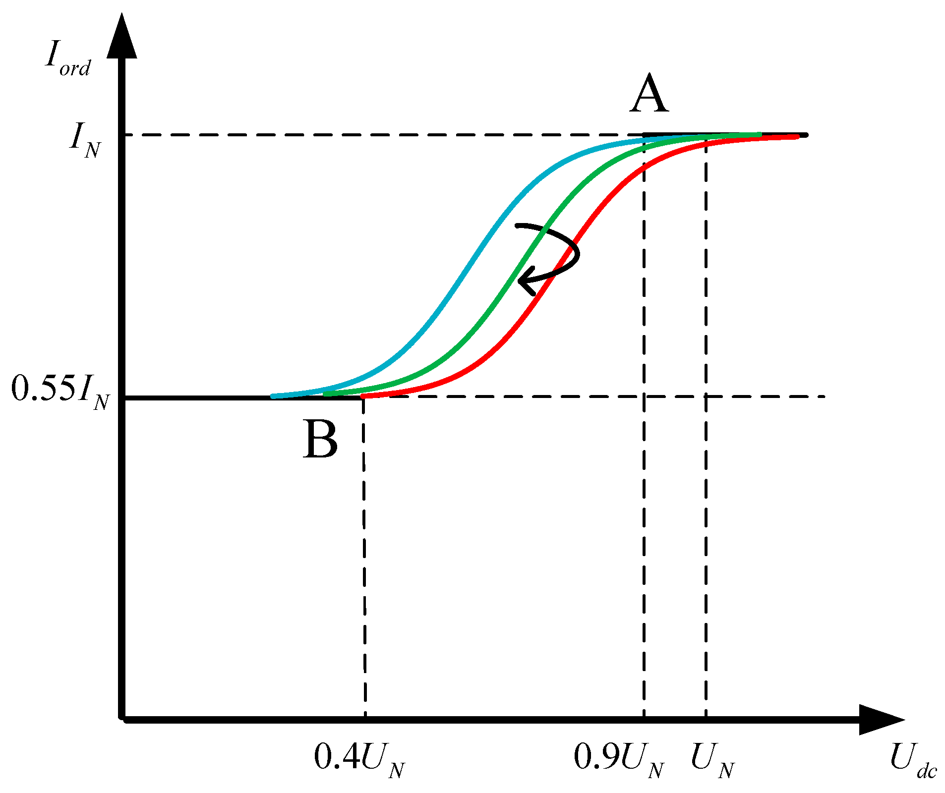
4. Nonlinear Dynamic VDCOL Control Strategy

In the event of a system commutation failure, the voltage stability and power recovery characteristics of the system are significantly affected by the VDCOL control parameters. Since the linear relationship between voltage and current of the normal VDCOL, the fixed slope of the VDCOL curve results in a low sensitivity of the DC current command. Further, after removing the fault, either too fast or too slow, an increase in the current command value of the VDCOL can affect the recovery of system power. The rapid growth of direct current will greatly increase the reactive power loss of the power system. In the case of the system not being able to obtain sufficient reactive power, the system voltage falls again, thus easily causing the subsequent commutation failure of the system, which is not conducive to the restoration of the system power. DC currents that increase too slowly cause a reduction in the active power transfer capability of the system, which is not conducive to maintaining a stable system power angle. Therefore, reasonable adjustment of the control parameters of the VDCOL is conducive to maintaining system voltage stability, suppressing phase commutation failure, and accelerating system power recovery.

Based on the above principles, a dynamic nonlinear VDCOL control strategy based on a Logistic function is designed in this paper between Point A and Point B, which is the process of fault recovery, as shown in the red part in Figure 4.

(1)

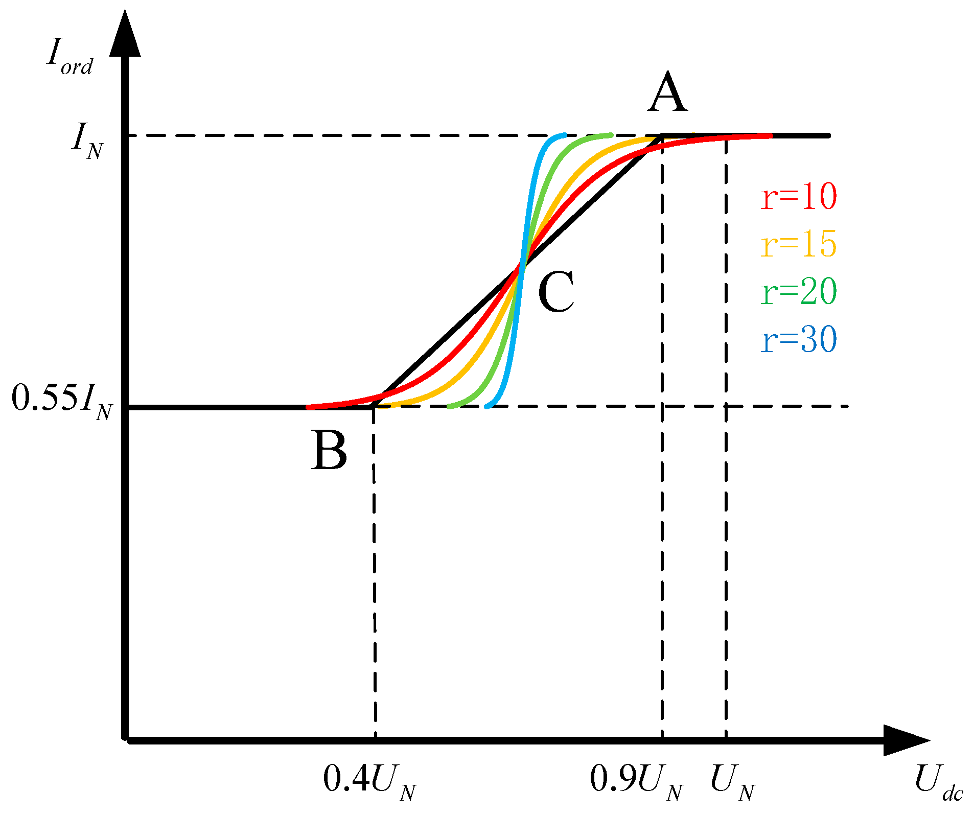
At the beginning of the first phase commutation failure, the system voltage drop is serious at a low level. To avoid weakening the stability of the system voltage due to the rapid recovery of the system DC power transfer, the DC current command value of the VDCOL is designed to be small and should be relatively smooth during the gradual recovery.

(2)

In the middle of the first phase commutation failure, the system voltage is recovered to a higher level. The conditions for fast recovery are in place to smoothly increase the DC current and restore the system power transfer, so the current command value of the design VDCOL curve rises at a faster rate.

(3)

At the anaphases of the first phase commutation failure, the system voltage recovers close to the normal level. In order to achieve a smooth transition of the system from transient to steady state and to reduce the system power interaction, the DC current command of the VDCOL output is designed to have a larger value, and the recovery process is smooth.

The expression for the voltage-current characteristic curve of the dynamic nonlinear VDCOL based on the logistic function is given as:

$$I_{ord}=\left\{\begin{array}{ll}0.55 \mathrm{p.u.}\hfill & U_{dc}<0.4 \mathrm{p.u.}\\ 0.45\times \frac{0.5\times e^{r(U_{dc}-\Delta U_o)}}{1+0.5\times (e^{r(U_{dc}-\Delta U_o)}-1)}+0.55 \mathrm{p.u.}\hfill & 0.4 \mathrm{p.u.}<U_{dc}<0.9 \mathrm{p.u.}\\ 1 \mathrm{p.u.}\hfill & U_{dc}>0.9 \mathrm{p.u.}\end{array}\right.$$

(12)

In Equation (12), $r$ is a fixed constant that measures the rate of change of the curve. In order to achieve a better adaptive effect, the fixed constant coefficient $r$ is usually chosen to range $10\le r\le 20$. The curves of the VDCOL function at different $r$ are shown in Figure 5. As shown in Figure 5, VDCOL activated at Point A, power transfer maintained at Point B and Point C is the midpoint of the logistic function. The black line in Figure 5 is the original VDCOL control strategy. When $r=10$, the rate of change of the dynamic nonlinear VDCOL control is minimized, which helps to reduce the fluctuation of the DC current command $I_{ord}$.

In Equation (12), $\mathsf{\Delta }{U}_o$ is the fault dynamic offset of the dynamic nonlinear VDCOL curve. As shown in Figure 5, it is necessary to introduce the fault degree factor $k$ to define the fault dynamic offset $\mathsf{\Delta }{U}_o$ since the fault voltage dynamic offset changes at point C during the commutation fault. Define the fault voltage dynamic offset $\mathsf{\Delta }{U}_o$ as

$$\Delta U_o=0.45+k$$

(13)

The fault degree factor, $k$, can be dynamically adjusted to the dynamic offset of the fault voltage according to the change of AC bus voltage during the fault. The expression of the fault degree factor $k$ is as follows:

$$k=1-\frac{U_{ac}}{U_{acN}},0\le k\le 1$$

(14)

where $U_{ac}$ is the actual RMS of the phase voltage of the AC bus at the inverter side; $U_{acN}$ is the rated value of the phase voltage of the AC bus at the inverter side.

The curves of nonlinear dynamic VDCOL constructed in this paper are shown in Figure 6. As shown in Figure 6, VDCOL activated at Point A, power transfer maintained at Point B and the arrows indicate the trajectory of the VDCOL curves.

When the system is operating normally, the fault degree factor $k=0$, VDCOL is the blue curve, as shown in Figure 6, the DC current command of the dynamic nonlinear VDCOL output $I_{ord}=1 \mathrm{p.u.}$, therefore, the normal operation of the system is not affected. When a fault occurs on the AC bus, the fault dynamic offset $\mathsf{\Delta }{U}_o$ at this time varies with the fault degree factor $k$, so the dynamic nonlinear VDCOL curve takes a left and right translation according to the fault severity. In the early stages of the fault, the system voltage dips severely, and the DC current rises sharply. At this point, the fault degree factor $k$ gradually increases, and the dynamic nonlinear VDCOL curve takes the right translation, the VDCOL curve is shifted from blue to green and then to red, as shown in Figure 6, in order to increase the current command response speed, decrease the current command $I_{ord}$, and reduce the power transfer, thus suppressing the occurrence of commutation failure. With the gradual recovery of the system voltage, the fault degree factor $k$ will gradually decrease, and the dynamic nonlinear VDCOL curve will be shifted to the left, the VDCOL curve is shifted from red to green and then to blue color, as shown in Figure 6, so that the DC current command $I_{ord}$ can be adjusted steadily and orderly according to the system voltage level, and the reactive power loss can be reduced, which is conducive to the recovery and transmission of the system power.

5. Simulation Verification

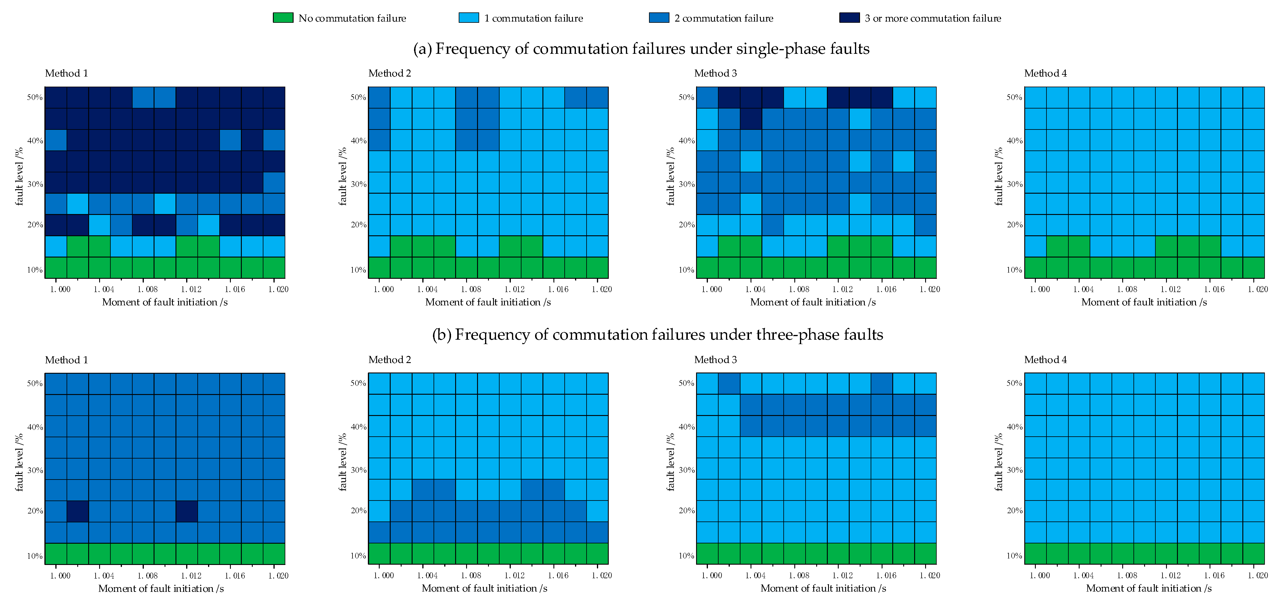
5.1. Comparison and Analysis of Methods

The effectiveness of the Method proposed in this paper is tested in the PSCAD/EMTDC using the CIGRE standard model. The CIGRE standard model is shown in Figure 7. The arrow points to the direction of power transfer in Figure 7. The parameters of the CIGRE standard test model are shown in

Table 3. The parameters of the CIGRE standard test model.

Parameters	Rectifier Side	Inverter Side
Reactive Power Compensation Capacity	626 Mvar	626 Mvar
AC System Parameters	382.87 kV,	215.05 kV,
	47.6 ∠ 84°Ω,	21.2 ∠ 75°Ω,
	SCR = 2.5	SCR = 2.5
Transformer Converter	603.87 MVA,	591.79 MVA,
	$X_T$ = 0.18 p.u.,	$X_T$ = 0.18 p.u.,
	345/213.5 kV	230/209.2 kV

.

In order to verify the effectiveness of our proposed strategies, we set up the following three control strategies in the HVDC test model:

Method 1: VDCOL control strategy of CIGRE test model

Method 2: VDCOL control strategy in Ref. [32]

Method 3: The nonlinear dynamic VDCOL control strategy constructed in this paper.

Method 4: Nonlinear dynamic VDCOL control strategy for DC voltage Taylor expansion based on Method 3.

Condition 1: The single-phase ground fault with a 0.2 H inductance is set up at the AC bus on the inverter side, with a fault start time of 1.0 s and a fault duration of 0.5 s. The electrical quantities of the system under the above four control Methods are shown in Figure 8.

In practical engineering, it is usually considered that the smaller the grounding inductance, the more serious the short-circuit fault. The grounding inductance $L_f=0.2H$ of Condition 1 can be considered as a single-phase grounding with a small inductance for more serious fault conditions. As can be seen from the change of extinction angle in Figure 8f, after a single-phase ground fault occurs in the system at 1.0 s, the extinction angle of the inverter-side of the system under the control of the above four Methods falls rapidly to 0°, at which time the first commutation failure occurs in all of them. During system recovery, subsequent commutation failures occurred in both Methods 1 and 3, while Method 2 and Method 4 gradually returned to a steady state at the extinction angle after the first commutation failure without any subsequent commutation failures occurred. However, Method 2 is on the verge of commutation failure as the actual extinction angle approaches the minimum extinction angle during subsequent recovery. During system recovery, the area Method 1 required for commutation is much larger than the area provided by the system due to the sharp rise in the DC current, so that the extinction angle falls to 0° again, and thus the system occurs a subsequent commutation failure. In Figure 8a, the system DC voltage under Method 2 control recovers fastest, but in Figure 8c,d, the fluctuations in the start-up voltage and current command values are large, with the risk of developing a subsequent commutation failure. At the beginning of the process of recovery, the electrical quantities of the system under Method 3 are similar to those of Method 1, but the system is able to quickly regulate the current command of the DC current with the nonlinear VDCOL control strategy proposed in this paper, as shown in Figure 8d, which play a limited role in suppressing the subsequent commutation failures. From Figure 8a–e, DC current under the control of Methods 3 and 4 recovered faster. It can be seen that during the occurrence of the first commutation failure of the system, not only the fluctuation of the DC current and voltage is reduced, but also the large drop of the VDCOL input voltage is suppressed, and the DC power loss is reduced, due to the fact that the Method 3 give more thought to the effect of compensation about DC voltage change than Method 2 during the system failure. After the first phase commutation failure of the system, under the four control Methods described above, Method 2 and Method 4 are effective in suppressing subsequent commutation failure under single-phase ground faults. However, Method 4 has less fluctuation in starting voltage and current command with better stability of DC current and voltage, and the extinction angle can be quickly restored to a stable state, which can effectively suppress the subsequent commutation failure and thus improve the stability of the system operation, so Method 4 has a strong adaptability to the single-phase faults of the subsequent commutation failure.

Condition 2: The three-phase ground fault with a 0.6 H inductance is set up at the AC bus on the inverter side, with a fault start time of 1.0 s and a fault duration of 0.5 s. The electrical quantities of the system under the above four control Methods are shown in Figure 9.

The grounding inductance $L_f=0.6H$ of Condition 2 can be considered as a three-phase inductive grounding with medium fault conditions. As can be seen from the turn-off angle waveform in Figure 9f, after a three-phase ground fault occurs in the system at 1.0 s, the first commutation failure occurs in all the above three control Methods. In the subsequent recovery process, the subsequent commutation failure occurs only in Method 1, while the extinction angles of Methods 2 and 3 do not fall below the critical extinction angle again. Therefore, the dynamic nonlinear VDCOL control strategy is effective in suppressing the subsequent commutation failure under a three-phase ground fault. Since Method 3 considers greater compensation of DC voltage change than Method 2 and reduces DC current and voltage fluctuation during system fault, the fluctuation amplitude of the extinction angle of Method 3 is smaller than that of Method 2, and the power transfer can quickly recover the stability, so Method 3 has strong adaptability for suppressing the subsequent commutation failure of three-phase fault. The grounding inductance $L_f=0.6H$ of Condition 2 can be considered as a three-phase inductive grounding with medium fault conditions. As can be seen from the turn-off angle waveform in Figure 9f, after a three-phase ground fault occurs in the system at 1.0 s, the first commutation failure occurs in all the above four control Methods. In the subsequent recovery process, the subsequent commutation failure occurs only in Method 1, while the extinction angles of Methods 2, Method 3, and Method 4 do not fall below the critical extinction angle again. As a result, Methods 2, 3, and 4 are effective in suppressing subsequent commutation failures under three-phase ground faults, but Methods 2 and 3 are on the verge of commutation failures with close to the minimum extinction angles. As can be seen from Figure 9c VDCOL input voltage, due to the amount of DC voltage variation compensation considered in Methods 2 and 4, the large drop in the starting voltage of the VDCOL is effectively suppressed during system faults. As seen in Figure 9d, the fluctuation of the current command value is small, which is conducive to the stable recovery of the DC current. Method 2 and Method 4 each have advantages in terms of system DC voltage and DC current recovery, with Method 2 being the fastest in terms of DC voltage recovery, as seen in Figure 9a, and Method 4 being the fastest in terms of DC current recovery, as seen in Figure 9b. Compared with Method 2, the DC current and voltage profile of the system under the control of Method 4 has a reduced drop and better DC current voltage stability. In Figure 9e, Method 4 has the shortest recovery time of DC power, and Method 4 has the smallest fluctuation of extinction angle to quickly restore stability; thus, Method 4 is highly adaptable to suppress the subsequent failure of three-phase faulty phase change.

Since Method 2 and Method 4 consider the greater compensation of DC voltage change and reduce DC current and voltage fluctuation during system fault, the fluctuation amplitude of the extinction angle of Method 3 is smaller than that of Method 2, and the power transfer can quickly recover the stability, so Method 3 has a strong adaptability for suppressing the subsequent commutation failure of three-phase fault.

The voltage drops in the inverter-side AC bus, the phase shift, and the moment of AC system fault initiation all affect the phase commutation process. In order to fully assess the effectiveness of the control Methods proposed in this paper for suppressing subsequent commutation failures in HVDC systems, a detailed comparative analysis of the effectiveness of the above Methods in suppressing commutation failures at different fault severities is required.

The fault capacity $F_L$ is used to reflect the system fault severity, the larger the fault capacity $F_L$ is, the more serious the system fault is, and its expression is as follows:

$$F_L=\frac{U_{acN}{}^2}{P_N\omega L_f}\times 100\%$$

(15)

where $U_{acN}$ is the rated value of the phase voltage of the AC bus at the inverter side; $\omega$ is the angular frequency of the AC system; $L_f$ is the grounding inductance; $P_N$ is the rated power of the DC transmission system. In this part, we simulate the system under different severity of faults and record the frequency of commutation failure to verify the suppressing effect of the control strategy proposed in this paper on subsequent commutation failure. The single-phase and three-phase faults with faulted capacity varying from 10% to 50% are set up at the inverter-side converter buses. The fault start moment varies from 1.000 s to 1.020 s. The simulation results are shown in Figure 10, where Figure 10a and Figure 10b, respectively, indicate the frequency of commutation failures occurring in the system under single-phase faults and three-phase faults with different fault levels. In Figure 10. green indicates that no commutation failure occurs; light blue indicates that the frequency of commutation failures is 1; medium blue indicates that the frequency of commutation failures is 2; and dark blue indicates that the frequency of commutation failures is 3 or more times.

From the statistical results of the system fault test in Figure 10, it can be seen that:

In the case of single-phase ground fault, Methods 1 and 3 are effectless in suppressing the subsequent commutation failure, and the subsequent commutation failure occurs many times; Method 2 is effective in suppressing the subsequent commutation failure, but the subsequent commutation failure also occurs in the case of moderate fault; Method 4 has the best control effect and effectively suppresses the system from the subsequent commutation failure.

In the case of three-phase ground faults, Method 1 has the worst effect on suppressing the subsequent commutation failures, with many cases of subsequent commutation failures; Method 2 has an obvious suppression effect in the case of moderate faults, effectively suppressing the subsequent commutation failures, but in the case of mild faults, the suppression effect is poor, with many cases of the subsequent commutation failures; Method 3 has an obvious suppression effect in the case of mild faults, effectively suppressing the subsequent commutation failures, but in the case of moderate faults, the suppression effect is poor, with many cases of the subsequent commutation failures; and Method 4 has the best control effect, effectively suppressing the occurrence of the subsequent commutation failures in the system.

In summary, the color comparison between Method 1 and Method 3 reveals that the dynamic nonlinear VDCOL of Method 3 is able to suppress the subsequent commutation failure under minor and moderate three-phase ground faults, while the suppression is ineffective under other fault conditions; in contrast, Method 4 makes up for the unsatisfactory suppression effect of Method 3 under other fault conditions by increasing the compensation based on the Taylor Expansion of DC voltage for starting voltage. Compared with Method 2, the dynamic nonlinear VDCOL of Method 4 takes into consideration the effect of the current command at the end of fault recovery on the system power recovery, thus effectively suppressing the subsequent commutation failure of the system. In a word, Method 4 is highly adaptable for suppressing subsequent commutation failures.

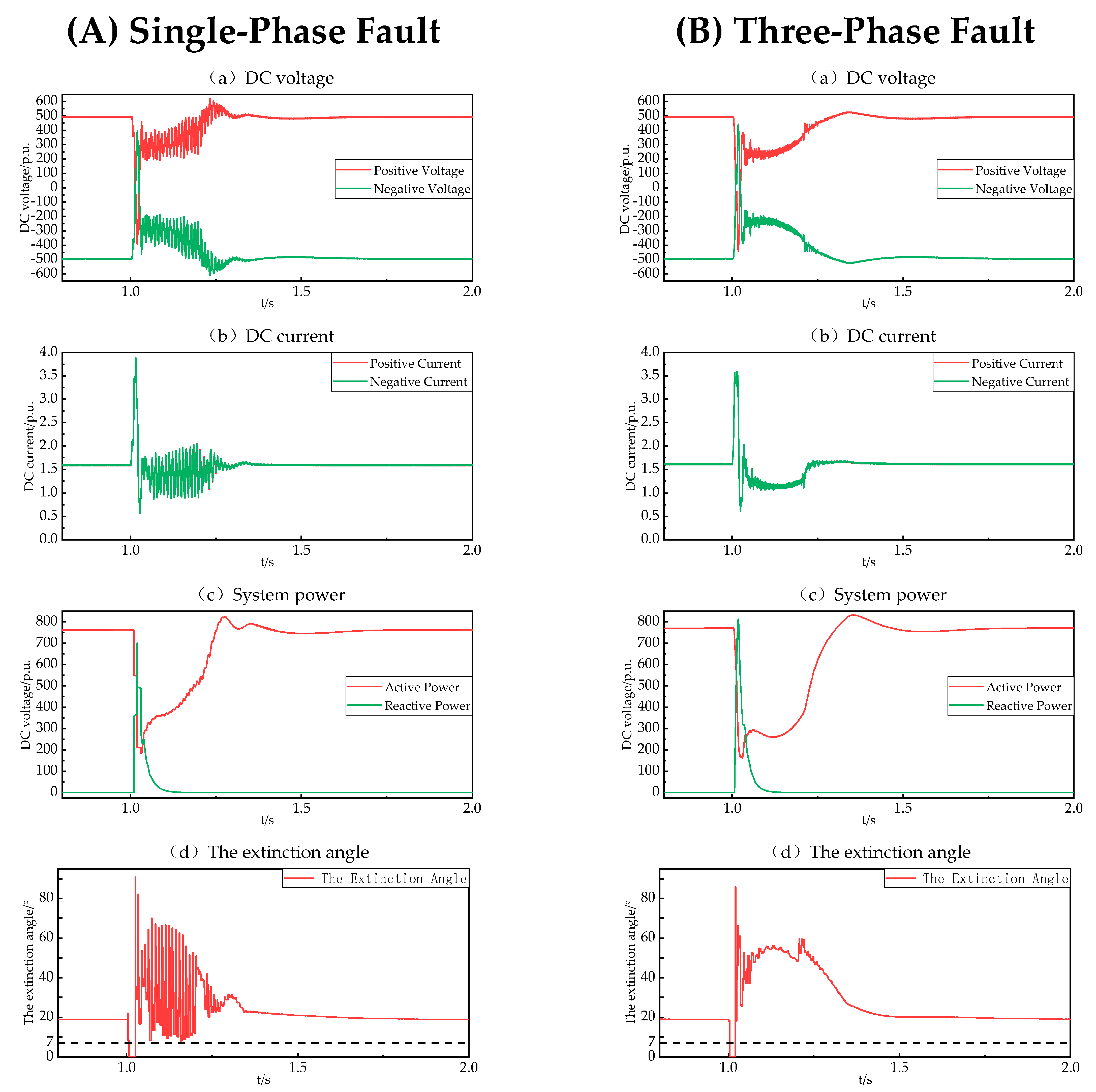
5.2. Simulation Verification Based on Actual Engineering

In order to fully verify the effectiveness of the proposed Method, the proposed control Method is simulated in the electromagnetic transient model built with the Tian Guang HVDC transmission system. The Tian Guang HVDC Transmission system model is shown in Figure 11. The arrow points to the direction of power transfer in Figure 11.

The actual parameters of The Tian Guang HVDC Transmission system are shown in

Table 4. The actual parameters of the Tian Guang HVDC transmission system.

Parameters	Tianshengqiao Converter Station	Guangzhou Converter Station
rated voltage/kV	230	230
Short circuit capacity/GVA	50	50
Equivalent Impedance/Ω	12.1	8.3
Equivalent Impedance Angle/°	4.372	6.370
Converter transformer capacity/MVA	84	84
Rated voltage of the converter transformer/kV	354/177/177	377/168.5/168.5
leakage resistance/%	$\frac{230}{\sqrt{3}}/208.6/\frac{208.6}{\sqrt{3}}$	$\frac{230}{\sqrt{3}}/198.5/\frac{198.5}{\sqrt{3}}$

.

Different types of short-circuit faults are set on the AC bus on the inverter side, and the fault duration is set to be 0.2 s, considering that fault durations are generally shorter in the actual system. Some of the electrical quantities of the Tian-Guang HVDC transmission system are shown in Figure 12.

In Figure 12(Ad,Bd), the dashed line represents the minimum extinction angle, i.e., commutation failure occurs when the actual extinction angle is lower than the dashed line. As can be seen in Figure 12, when a single-phase fault occurs in the inverter-side AC system, the extinction angle of the control strategy proposed in the paper only appears to drop to a state smaller than the minimum extinction angle once, and there is no subsequent commutation failure, which effectively suppresses the subsequent commutation failure. The degree of fluctuation of DC voltage, DC current, and system power is relatively small, and the recovery of the system after the failure is relatively fast. When a three-phase fault occurs in the system, the system is more effective in suppressing the subsequent commutation failure, and the recovery is more obvious. It is shown that the proposed dynamic nonlinear VDCOL control strategy based on Taylor Expansion of DC voltages can effectively suppress the Subsequent Commutation failure in the HVDC transmission and accelerate the recovery of the system after the fault.

6. Conclusions

Aiming at the subsequent commutation failure of the HVDC transmission system, this paper proposes a dynamic nonlinear VDCOL subsequent commutation failure control strategy based on the Taylor expansion of DC voltage, according to the mechanism of commutation failure and the principle of VDCOL control. Through extensive simulation analyses on the actual parametric model, the conclusions were obtained as follows:

(1)

A large drop in DC voltage, which causes sharp fluctuations in the DC current command value, is a key reason for subsequent commutation failure.

(2)

Considering the relationship between the change of DC current and system power recovery after a fault, the Method improves the stability of the current command by optimizing the starting voltage and constructing a dynamic nonlinear VDCOL. The Method effectively suppresses the subsequent commutation failures under different fault cases of single-phase and three-phase with good results on the stabilization and recovery of the DC system.

(3)

The Method is realized in the DC control system without incorporating physical electrical components in the engineering practices, as the result of significant cost savings. Moreover, it is easy to achieve without the need for additional auxiliary devices of electrical devices.

References

1. Zhao, W.J. High Voltage Direct Current Transmission Engineering Technology; China Electrical Power Press: Beijing, China, 2004. [Google Scholar]
2. Thio, C.V.; Davies, J.B.; Kent, K.L. Commutation failures in HVDC transmission systems. IEEE Trans. Power Deliv. 1996, 11, 946–957. [Google Scholar] [CrossRef]
3. Zhu, Y.N.; Zhang, S.Q.; Liu, D.; Zhu, L.; Zou, S.; Yu, S.Q.; Sun, Y.B. Prevention and mitigation of high-voltage direct current commutation failures: A review and future directions. IET Gener. Transm. Distrib. 2019, 13, 5449–5456. [Google Scholar] [CrossRef]
4. Yuan, Y.; Wei, Z.; Lei, X.; Wang, H.; Sun, G. Survey of commutation failures in DC transmission systems. Electr. Power Autom. Equip. 2013, 33, 140–147. [Google Scholar] [CrossRef]
5. Li, Y.; Liu, F.; Luo, L.F.; Rehtanz, C.; Cao, Y.J. Enhancement of Commutation Reliability of an HVDC Inverter by Means of an Inductive Filtering Method. IEEE Trans. Power Electron. 2013, 28, 4917–4929. [Google Scholar] [CrossRef]
6. Guo, C.Y.; Yang, Z.Z.; Jiang, B.S.; Zhao, C.Y. An Evolved Capacitor-Commutated Converter Embedded with Antiparallel Thyristors Based Dual-Directional Full-Bridge Module. IEEE Trans. Power Deliv. 2018, 33, 928–937. [Google Scholar] [CrossRef]
7. Gao, C.; He, Z.; Yang, J.; Sheng, C.; Zhang, J.; Wang, P. A Novel Controllable Line Commutated Converter Topology and Control Strategy. Proc. Chin. Soc. Electr. Eng. 2023, 43, 1940–1949. [Google Scholar] [CrossRef]
8. Gao, K.; Qu, H.; Ren, M.; Liu, Y.; Zeng, X.; Cao, J.; Cui, C.; Luo, Y. Commutation Failure Suppression Technology for HVDC Transmission Based on Controlled Voltage Source. High Volt. Appar. 2023, 59, 49–57. [Google Scholar] [CrossRef]
9. Rehman, A.U.; Guo, C.; Zhao, C. Coordinated Control for Operating Characteristics Improvement of UHVDC Transmission Systems under Hierarchical Connection Scheme with STATCOM. Energies 2019, 12, 945. [Google Scholar] [CrossRef]
10. Liu, Y.; Liu, J.; Gao, H. A Method for Optimizing the VDCOL Parameter to Suppress the Subsequent Commutation Failure of Multi-infeed HVDC System. Electr. Power Constr. 2021, 42, 122–129. [Google Scholar] [CrossRef]
11. Zhang, L.D.; Dofnas, L. A novel method to mitigate commutation failures in HVDC systems. In Proceedings of the International Conference on Power System Technology, Kunming, China, 13–17 October 2002; pp. 51–56. [Google Scholar] [CrossRef]
12. Liu, L.; Li, X.; Teng, Y.; Zhang, C.; Lin, S. An enhanced commutation failure prevention control in LCC based HVDC. Int. J. Electr. Power Energy Syst. 2023, 145, 108584. [Google Scholar] [CrossRef]
13. Xiao, C.; Xiong, X.; Ouyang, J.; Ma, G.; Zheng, D.; Tang, T. A Commutation Failure Suppression Control Method Based on the Controllable Operation Region of Hybrid Dual-Infeed HVDC System. Energies 2018, 11, 574. [Google Scholar] [CrossRef]
14. Zhao, J.; Li, X.; Wang, Y.; Tan, Z.; Wang, J.; Cai, Z. Continuous commutation failure suppression strategy based on firing angle deviation compensation. Electr. Power Autom. Equip. 2023, 43, 210–216. [Google Scholar] [CrossRef]
15. Cong, X.; Zheng, X.; Cao, Y.; Tai, N.; Miao, Y.; Li, K. A Suppression Strategy for Subsequent Commutation Failures Considering Commutation Capability of Recovery Process. J. Shanghai Jiaotong Univ. 2022, 56, 333–341. [Google Scholar]
16. Cai, H.; Li, J.; Zhou, Y.; Hu, Y. An Adaptive Phase Locked Oscillator to Improve the Performance of Fault Recovery from Commutation Failure in LCC-Based HVDC Systems. Energies 2023, 16, 5299. [Google Scholar] [CrossRef]
17. Yu, Z.; Wang, J.; Fu, C.; Wu, Q.; Liu, Y.; Li, X. An Improved HVDC Synchronous Firing Control Method Based on Order Switching and Phase Compensation. IEEE Trans. Power Deliv. 2023, 38, 966–978. [Google Scholar] [CrossRef]
18. Liu, X.; Cao, Z.; Gao, B.; Zhou, Z.; Wang, X.; Zhang, F. Predictive Commutation Failure Suppression Strategy for High Voltage Direct Current System Considering Harmonic Components of Commutation Voltage. Processes 2022, 10, 2073. [Google Scholar] [CrossRef]
19. Ying, F.U.; Longfu, L.U.O.; Ze, T.; Yong, L.I.; Jinping, Z.; Jiazhu, X.U.; Fusheng, L.I.U. Study on Voltage Dependent Current Order Limiter of HVDC Transmission System’s Controller. High Volt. Eng. 2008, 34, 1110–1114. [Google Scholar] [CrossRef]
20. Hong, L.R.; Zhou, X.P.; Liu, Y.F.; Xia, H.T.; Yin, H.H.; Chen, Y.D.; Zhou, L.M.; Xu, Q.M. Analysis and Improvement of the Multiple Controller Interaction in LCC-HVDC for Mitigating Repetitive Commutation Failure. IEEE Trans. Power Deliv. 2021, 36, 1982–1991. [Google Scholar] [CrossRef]
21. Li, R.; Li, Y.; Chen, X. A Control Method for Suppressing the Continuous Commutation Failure of HVDC Transmission. Proc. Chin. Soc. Electr. Eng. 2018, 38, 5029–5042. [Google Scholar] [CrossRef]
22. Cao, S.; Wei, F.; Lin, X.; Li, Z.; Jiang, Y.; Chen, C.; Ma, Y.; Li, F. A commutation failure suppression strategy based on adaptive voltage limits. Power Syst. Prot. Control 2023, 51, 165–175. [Google Scholar] [CrossRef]
23. Zhang, W.; Xiong, Y.; Li, C.; Yao, W.; Wen, J.; Gao, D. Continuous commutation failure suppression and coordinated recovery of multi-infeed DC system based on improved VDCOL. Power Syst. Prot. Control 2020, 48, 63–72. [Google Scholar] [CrossRef]
24. Liu, X.; Wang, Z.; Zheng, B.; Wang, T.; Qiao, X. Mechanism Analysis and Mitigation Measures for Continuous Commutation Failure During the Restoration of LCC-HVDC. Proc. Chin. Soc. Electr. Eng. 2020, 40, 3163–3171. [Google Scholar] [CrossRef]
25. Cheng, F.; Yao, L.; Wang, Z.; Liu, C.; Wang, Q.; Deng, J.; Lan, T. A Commutation Failure Mitigation Strategy Based on Virtual Phase Lock Loop Voltage. Proc. Chin. Soc. Electr. Eng. 2020, 40, 2756–2765. [Google Scholar] [CrossRef]
26. Guo, C.; Li, C.; Liu, Y.; Jiang, B.; Zhao, C.; Zhou, Q. A DC Current Limitation Control Method Based on Virtual-resistance to Mitigate the Continuous Commutation Failure for Conventional HVDC. Proc. Chin. Soc. Electr. Eng. 2016, 36, 4930–4937. [Google Scholar] [CrossRef]
27. Lu, Y.; Tong, K.; Ning, L.; Xuan, J.; Guo, C.; Zhao, C. A Method Mitigating Continuous Commutation Failure for Double-Infeed HVDC System Based on Virtual Inductor. Power Syst. Technol. 2017, 41, 1503–1509. [Google Scholar] [CrossRef]
28. Song, H.; Han, K. Research on Suppressing Continuous Commutation Failure of HVDC System Based on Virtual Capacitor. In Proceedings of the 2021 IEEE/IAS Industrial and Commercial Power System Asia (I&CPS Asia), Chengdu, China, 18–21 July 2021; p. 721. [Google Scholar] [CrossRef]
29. Zhou, H.; Yao, W.; Li, C.; Wen, J. A Predictive Voltage Dependent Current Order Limiter with the Ability to Reduce the Risk of First Commutation Failure of HVDC. High Volt. Eng. 2022, 48, 3179–3189. [Google Scholar] [CrossRef]
30. He, D.; Wen, J.; Geng, X.; Wang, S.; Zhang, L.; Cai, Y.; Luo, Z.; Tan, M. Study on HVDC commutation failure and voltage compensated variable slope VDCOL control. In Proceedings of the 2018 2nd IEEE Conference on Energy Internet and Energy System Integration (EI2), Beijing, China, 20–22 October 2018; p. 6. [Google Scholar] [CrossRef]
31. Meng, Q.; Liu, Z.; Hong, L.; Zhou, X.; Xia, H.; Liu, Y.; Wang, X. A suppression method based on nonlinear VDCOL to mitigate the continuous commutation failure. Power Syst. Prot. Control 2019, 47, 119–127. [Google Scholar]
32. Zhu, H.; Li, Y.; Zhou, Z.; Zhu, H.; Qian, W. Design of a dynamic nonlinear VDCOL controller with additional virtual capacitance. Power Syst. Prot. Control 2022, 50, 134–143. [Google Scholar] [CrossRef]
33. Liu, L.; Wang, Y.; Li, X.; Zhang, B. Design of Variable Slope VDCOL Controller Based on Fuzzy Control. Power Syst. Technol. 2015, 39, 1814–1818. [Google Scholar] [CrossRef]
34. Feng, M.; Li, X.; Li, N.; Wang, C.; Hong, C. Study of HVDC Piecewise Variable Rate VDCOL Based on Simplex Algorithm. J. Sichuan University. Eng. Sci. Ed. 2015, 47, 162–167. [Google Scholar] [CrossRef]
Figure 1. The model of the commutation process.
Energies 16 07342 g001
Figure 2. The characteristic curve of Normal VDCOL.
Energies 16 07342 g002
Figure 3. Optimization of starting voltage structure diagram.
Energies 16 07342 g003
Figure 4. The characteristic curve of VDCOL based on the Logistic function.
Energies 16 07342 g004
Figure 5. The curve of VDCOL at r .
Energies 16 07342 g005
Figure 6. Characteristic curve of Nonlinear dynamic VDCOL.
Energies 16 07342 g006
Figure 7. The CIGRE standard test model.
Energies 16 07342 g007
Figure 8. System operating characteristics under single-phase ground fault L f = 0.2 H ; (a) Curve of variation of DC voltage; (b) Curve of variation of DC current; (c) Curve of variation of the starting voltage; (d) Curve of variation of the current command of VDCOL; (e) Curve of variation of DC power; (f) Curve of variation of the extinction angle.
Energies 16 07342 g008
Figure 9. System operating characteristics under three-phase ground fault L f = 0.6 H ; (a) Curve of variation of DC voltage; (b) Curve of variation of DC current; (c) Curve of variation of the starting voltage; (d) Curve of variation of the current command of VDCOL; (e) Curve of variation of DC power; (f) Curve of variation of the extinction angle.
Energies 16 07342 g009
Figure 10. Test of fault suppression ability; (a) Frequency of commutation failures under single-phase faults; (b) Frequency of commutation failures under three-phase faults.
Energies 16 07342 g010
Figure 11. The Tian Guang HVDC Transmission system model.
Energies 16 07342 g011
Figure 12. The electrical quantities of the Tian-Guang HVDC transmission system; (A) Tian Guang HVDC transmission system under single-phase fault; (B) Tian Guang HVDC transmission system under three-phase fault.
Energies 16 07342 g012